Estimates of isospin breaking contributions to baryon masses

Abstract

We estimate the isospin breaking contributions to the baryon masses which we analyzed recently using a loop expansion in the heavy baryon approximation to chiral effective field theory. To one loop, the isospin breaking corrections come from the effects of the $d,\,u$ quark mass difference, the Coulomb and magnetic moment interactions, and effective point interactions attributable to color-magnetic effects. The addition of the first meson loop corrections introduces new structure. We estimate the resulting low-energy, long-range contributions to the mass splittings by regularizing the loop integrals using connections to dynamical models for finite-size baryons. We find that the resulting contributions to the isospin breaking corrections are of the right general size, have the correct sign pattern, and agree with the experimental values within the margin of error.

I Introduction

In a recent paper Durand and Ha (2005), we analyzed the structure of the electromagnetic contributions to the mass splittings within isospin multiplets in the baryon octet and decuplet. In particular, we studied the leading isospin breaking (IB) contributions to the mass differences that come from the Coulomb and magnetic interactions, quark mass differences, and the one-loop mesonic corrections to those interactions.

Our analysis was based on the standard chiral Lagrangian in the heavy baryon approximation (HBA) to chiral effective field theory as developed by Georgi Georgi (1990) and Jenkins and Manohar Jenkins and Manohar (1991). However, we used a spin- and flavor-index or “quark” representation of the effective octet and decuplet baryon fields and the electromagnetic and mesonic interactions rather than the usual matrix expressions for the fields. The connection of this representation to the usual effective-field methods was discussed in detail in Durand et al. (2001, 2002). It has been applied in past analyses of the splittings between baryon isospin multiplets Durand et al. (2001, 2002); Ha and Durand (1999), and of the baryon magnetic moments Durand et al. (2002); Ha and Durand (2003). The results in each case can be summarized in terms of a set of effective interactions that have the appearance of interactions between quarks in the familiar semirelativistic or nonrelativistic quark models for the baryons. The results are in fact completely general in their representation of the relativistic heavy-baryon effective fields and their interactions as shown in Durand et al. (2001, 2002). In the present case, our results connect directly to Morpurgo’s general parametrization of the electromagnetic effects Morpurgo (1992) derived from QCD.

Our derivations in Durand and Ha (2005) included the one-loop mesonic corrections to the basic one-loop electromagnetic interactions, so involved two loops overall. We derived a complete expression for the isospin breaking electromagnetic contributions to the baryon mass operator to this order, and then used the result to obtain expressions for the operators that lead to intramultiplet mass splittings. As indicated, our emphasis was on the loop expansion, rather than on the splittings obtained in a perturbative expansion in powers of the chiral symmetry breaking parameters as in Muller and Meissner (1999). The Feynman loop integrals that appear in the final results are of course the same as those obtained using the usual effective fields, but have been reduced in Durand and Ha (2005) for loops containing heavy baryons to integrals for time-ordered graphs.

It remains to obtain explicit expressions for the mass splittings, calculate the integrals that appear, and compare the results with experiment, the subjects of the present paper. We will do this by using the natural connection of the “quark” description of the effective fields to semirelativistic dynamical models with the effective quarks playing the role of structure quarks. This will allow us to model the structure of the matrix elements beyond the point-baryon approximation and estimate the matrix elements of the effective Hamiltonian for finite-size baryons. The results will necessarily be model-dependent, but can be regarded as involving physically-motivated choices of cutoffs that emphasize the calculable long-distance parts of the loop corrections in the sense discussed by Donoghue, Holstein, and Borasoy Donoghue et al. (1999).

The electromagnetic contributions to the baryon masses can be expressed as a linear combination of the matrix elements of a set of independent spin- and flavor-dependent operators $\Gamma_{i}$, $(i=1,...,32)$ in the baryon states . There are 2 independent operators that involve only one set of quark indices, called one-body operators, 12 two-body operators, and 18 three-body operators.

We showed in Durand and Ha (2005) that no three-body operators are generated by one-loop mesonic corrections to the initial two-body Coulomb and magnetic moment interactions after renormalization, even though diagrams that connect three sets of quark indices are initially present. The number of $\Gamma$’s that can appear to this order is therefore reduced from 32 to 14. When the calculation is restricted to the intramultiplet splittings, the number of independent matrix elements is further reduced to 4 Durand and Ha (2005); Morpurgo (1989); Dillon and Morpurgo (2000). As a result, we can bring the electromagnetic mass-difference operator to the form

$$\mathcal{H}_{\textrm{IB}}=a\sum_{i}M^{d}_{i}+b\Gamma_{4}+c\Gamma_{5}+d\Gamma_{13}\,,$$ (1)

where

$$\Gamma_{4}=\frac{1}{2}\sum_{i\not=j}\,Q_{i}Q_{j}\,,\,\,\Gamma_{5}=\frac{1}{2}\sum_{i\not=j}\,Q_{i}Q_{j}\bm{\sigma}_{i}\cdot\bm{\sigma}_{j}\,,\,\,\Gamma_{13}=\frac{1}{2}\sum_{i\not=j}\,Q_{i}Q_{j}M_{j}^{s}\,,\,\,$$

the $Q$s are quark charge matrices, and the matrices $M^{d}$ and $M^{s}$ are defined as $M^{d}=\textrm{diag}\,(0,1,0)$, $M^{s}=\textrm{diag}\,(0,0,1)$ . The complete set of one- and two- body electromagnetic operators is given in Appendix A. The procedures needed to convert Eq. (1) to an expression in terms of effective baryon fields in the matrix representation are described in detail in Durand et al. (2001, 2002), but will not be needed here.

As will be discussed in Sec. II, the results in Durand and Ha (2005) omitted two further isospin breaking contributions proportional to $m_{d}-m_{s}$ that are allowed by the general effective field theory. These are analogous to the effective point interactions of the form $\sum\bm{\sigma}_{i}\cdot\bm{\sigma}_{j}M^{s}_{i}$ and $\sum\bm{\sigma}_{i}\cdot\bm{\sigma}_{j}M^{s}_{i}M^{s}_{j}$ that appeared in our earlier analysis of intermultiplet mass splittings Durand et al. (2001, 2002), but involve the replacement of (one) matrix $M^{s}$ by $M^{d}$ and have coefficients proportional to the mass difference $(m_{d}-m_{u})$ rather than $m_{s}$. As shown below, terms of this form arise in QCD-based dynamical models from a color-magnetic interaction Zel’dovich and Sakharov (1967), and can give IB contributions to the intramultiplet mass splittings comparable to those from electromagnetic interactions Sakharov (1980); Franklin and Lichtenberg (1982) . Since the extra effective interactions are two-body, the usual quark-model sum rules Rubenstein (1966); Rubenstein et al. (1967); Gal and Scheck (1967) for baryon masses continue to hold for matrix elements. Once again, only four parameters $a$, $b$, $c$, and $d$ are needed to describe the intramultiplet mass splittings through first order in $(m_{d}-m_{u})$, corresponding to an effective interaction of the form in Eq. (1).

Our objectives in the present paper are, first, to extend the theoretical analysis of isospin breaking mass splittings by including the effects of the “color-magnetic” interactions Zel’dovich and Sakharov (1967) missed in Durand and Ha (2005), and, second, to estimate the final coefficients $a$, $b$, $c$, and $d$ in $\mathcal{H}_{\textrm{IB}}$ numerically in the heavy baryon approximation. The first part of the analysis is completely general. The second will depend on specific models for baryon structure.

As shown explicitly in Sec. II.3, the electromagnetic contributions to the coefficients $a$, $b$, $c$, and $d$ are given by combinations of cutoff-dependent Feynman integrals over the three momenta in pion and photon loops. The effect of the soft, long-range parts of the interactions are expected to be calculable. We will therefore make reasonable estimates of the soft parts of the integrals by employing known form factors and dynamical models in cutting off the divergent integrals. The differences from the experimental values give estimates of the sizes of the residual hard, short-range contributions.

With the color-magnetic interaction included, we find that the calculated IB corrections are of the right general size and have the correct sign pattern to account for the pattern of the coefficients in the IB mass-difference Hamiltonian. The theoretical results agree with their experimental values at or within the margin of error, especially given the uncertainty in the theoretical input. Unless the corrections in the chiral expansion from two meson loops (three loops overall) are larger than we would expect, any deviations from the experiment can be attributed to the presence of short-distance effects which can be parametrized but not calculated in the effective field theory.

II Isospin breaking corrections to baryon masses

It is necessary to recall that the leading IB corrections to baryon masses come from the Coulomb interaction, magnetic moments interactions, the effects of the $d,\,u$ quark mass difference, and the color-magnetic interaction. We note that except for the color-magnetic interaction, we have included the one-loop mesonic corrections to other basic electromagnetic interactions (two loops overall) in our calculations. We wish to evaluate the contributions from these effects to the parameters $a$, $b$, $c$, and $d$. For this goal, we firstly discuss the contributions from the color-magnetic interaction to the mass splittings.

II.1 Color-magnetic contributions

The QCD color-magnetic interaction was first introduced by Sakharov and Zel’dovich Zel’dovich and Sakharov (1967) and further developed by De Rújula, Georgi, and Glashow A. De Rújula and Glashow (1975) for their study on hadron masses in a gauge theory. Sakharov Sakharov (1980) and Franklin and Lichtenberg Franklin and Lichtenberg (1982) showed that the QCD color-magnetic interaction was of the same order of magnitude as the purely electromagnetic interaction. The color-magnetic contributions to the mass of a baryon $B$ arise in relativistic quark models from the interaction

$$\mathcal{H}_{\textrm{CM}}^{B}=\frac{4\pi\alpha_{s}}{9}\left[\frac{\bm{\sigma}_{i}\cdot\bm{\sigma}_{j}}{m_{i}m_{j}}\,\delta^{3}(\bm{r}_{ij})+(j,k)+(k,i)\right]\,,$$ (2)

where $m_{i}$, $m_{j}$ represent effective quark masses, and $\alpha_{s}$ is the strong coupling. At this point we will not attempt to calculate the matrix elements of this interaction, but will simply use its spin and mass structure to determine the equivalent effective operators to use with the heavy-baryon effective fields. We want, in particular, to see the extent to which the interaction in (Eq. (2)) can be reduced to an operator expression in terms of the $\Gamma$’s and $M^{d}$. For that purpose, we take $m_{u}$ as the standard mass and consider the symmetrical case in which $<\delta^{3}(\bm{r}_{ij})>\equiv A$, a constant, for all states. We then substitute the identity

$$\frac{1}{m_{i}} = \frac{1}{m_{u}}\left[M^{u}+\frac{m_{u}}{m_{d}}M^{d}+\frac{m_{u}}{m_{s}}M^{s}\right]_{i}$$ (3)

$$= \frac{1}{m_{u}}\left[\openone+\frac{m_{u}-m_{d}}{m_{d}}M^{d}+\frac{m_{u}-m_{s}}{m_{s}}M^{s}\right]_{i}$$

into Eq. (2) and expand. To first order in $m_{d}-m_{u}$, the color-magnetic interaction can then be rewritten as

$$\mathcal{H}_{\textrm{CM}}^{B}=-C\sum_{i\not=j}\,M_{i}^{d}\bm{\sigma}_{i}\cdot\bm{\sigma}_{j}+C^{\prime}\sum_{i\not=j}M_{i}^{d}M_{j}^{s}\bm{\sigma}_{i}\cdot\bm{\sigma}_{j}+\ldots\,,$$ (4)

where

$$C=\frac{4\pi\alpha_{s}}{9}\frac{A}{m_{u}^{2}}\frac{m_{d}-m_{u}}{m_{u}}\,,\,\,\,C^{\prime}=C\frac{m_{s}-m_{u}}{m_{s}}\,,$$ (5)

and the ellipsis represents terms that can be absorbed into the structures that already appear in our analysis of intermultiplet mass splittings in Durand et al. (2002).

As mentioned above, the terms that are written out explicitly involve isospin-breaking operators of order $m_{d}-m_{u}$ that are allowed in the effective field theory and could have been introduced from the beginning with unknown coefficients to be determined from the data. The derivation suggests that these represent short-distance effects not calculable in the chiral expansion.

We now show how to put the color-magnetic interaction in the standard $a,b,c,d$ form. Using the identity

$$M^{d}=-3Q^{2}+\frac{4}{3}\openone-M^{s}\,,$$ (6)

we rewrite the operators in Eq. (4) as

$$\sum_{i\not=j}M_{i}^{d}\bm{\sigma}_{i}\cdot\bm{\sigma}_{j}=\frac{4}{3}\sum_{i\not=j}\bm{\sigma}_{i}\cdot\bm{\sigma}_{j}-\sum_{i\not=j}M_{i}^{s}\bm{\sigma}_{i}\cdot\bm{\sigma}_{j}-6\Gamma_{2},$$ (7)

$$\sum_{i\not=j}M_{i}^{d}M_{j}^{s}\bm{\sigma}_{i}\cdot\bm{\sigma}_{j}=\frac{4}{3}\sum_{i\not=j}M_{j}^{s}\bm{\sigma}_{i}\cdot\bm{\sigma}_{j}-\sum_{i\not=j}M_{i}^{s}M_{j}^{s}\bm{\sigma}_{i}\cdot\bm{\sigma}_{j}-6\Gamma_{11}.$$ (8)

The first two operators on the right in each expression contribute to intermultiplet splittings but not to isospin splittings within multiplets, so these can be dropped. As far as the splittings are concerned, the following relations hold

$$\Gamma_{2}=\frac{1}{3}\sum_{i}M_{i}^{d}+\frac{1}{2}(\Gamma_{4}-\Gamma_{5})\,,\,\,\,\Gamma_{11}=-\Gamma_{13}+\frac{1}{2}(\Gamma_{4}-\Gamma_{5})\,.$$

Hence, we find

$$\mathcal{H}_{\textrm{CM}}^{B}=a_{\rm{CM}}\sum_{i}M^{d}_{i}+b_{\rm{CM}}\Gamma_{4}+c_{\rm{CM}}\Gamma_{5}+d_{\rm{CM}}\Gamma_{13}\,,$$ (9)

where

$$a_{\rm{CM}}=-2C\,,\,\,b_{\rm{CM}}=3(C-C^{\prime})\,,\,\,c=-3(C-C^{\prime})\,,\,\,d=6C^{\prime}\,.$$ (10)

Note that the sum rules for baryon masses continue to hold Rubenstein (1966); Rubenstein et al. (1967); Gal and Scheck (1967).

The one-loop mesonic corrections to the effective point interactions do not introduce new isospin breaking terms, are expected to be small, and will not be considered.

II.2 Baryon mass splittings and sum rules

The contributions of the operators $\sum_{i}M^{d}_{i}$, $\Gamma_{4}$, $\Gamma_{5}$, and $\Gamma_{13}$ to the mass splittings within baryon multiplets can be determined from the results given in Durand and Ha (2005); Morpurgo (1989). Using those results (see, for example, Table I of the reference Durand and Ha (2005) ) and Eq. (1), we find

$$n-p = a-\frac{b}{3}-\frac{c}{3}\,,$$

$$\Sigma^{-}-\Sigma^{+} = 2a+\frac{b}{3}-\frac{5c}{3}+\frac{d}{3}\,,$$

$$\Sigma^{-}-\Sigma^{0} = a+\frac{2b}{3}-\frac{c}{3}+\frac{d}{6}\,,$$

$$\Xi^{-}-\Xi^{0} = a+\frac{2b}{3}-\frac{4c}{3}+\frac{d}{3}\,,$$

$$\Sigma^{*-}-\Sigma^{*+} = 2a+\frac{b}{3}+\frac{c}{3}+\frac{d}{3}\,,$$ (11)

$$\Sigma^{*-}-\Sigma^{*0} = a+\frac{2b}{3}+\frac{2c}{3}+\frac{d}{6}\,,$$

$$\Xi^{*-}-\Xi^{*0} = a+\frac{2b}{3}+\frac{2c}{3}+\frac{d}{3}\,,$$

$$\Delta^{++}-\Delta^{0} = -2a+\frac{5b}{3}+\frac{5c}{3}\,,$$

$$\Delta^{++}-\Delta^{-} = -3a+b+c\,,$$

$$\Delta^{+}-\Delta^{0} = -a+\frac{b}{3}+\frac{c}{3}\,.$$

Since there are only four independent parameters in $\mathcal{H}_{\textrm{IB}}$, there are six sum rules among ten mass differences. Below are the well-known sum rules Coleman and Glashow (1961); Rubenstein (1966); Rubenstein et al. (1967); Gal and Scheck (1967); Ishida et al. (1966)

$$\Delta^{0}-\Delta^{+}=n-p\,,$$

$$\Delta^{-}-\Delta^{++}=3(n-p)\,,$$

$$\Delta^{0}-\Delta^{++}=2(n-p)+(\Sigma^{0}-\Sigma^{+})-(\Sigma^{-}-\Sigma^{0})\,,$$

$$\Xi^{-}-\Xi^{0}=(\Sigma^{-}-\Sigma^{+})-(n-p)\,,$$ (12)

$$\Xi^{*-}-\Xi^{*0}=(\Sigma^{*-}-\Sigma^{*+})-(n-p)\,,$$

$$2\Sigma^{*0}-\Sigma^{*+}-\Sigma^{*-}=2\Sigma^{0}-\Sigma^{+}-\Sigma^{-}.$$

These sum rules hold for any set of purely one- and two-body interactions as shown in Rubenstein (1966); Rubenstein et al. (1967); Gal and Scheck (1967); Ishida et al. (1966).

The sum rules can be violated by three-body operators. However, as shown in Durand and Ha (2005) and mentioned above, no effective three-body operators are generated through one loop in the chiral expansion, so any three-body effects must involve at least two meson loops and are expected to be small. The sum rules are therefore expected to hold with reasonable accuracy, as they do.

A weighted fit to the seven known mass splittings other than those for the $\Delta$ baryons is given in Table 1.

Table 1: A weighted fit to the seven accurately known baryon mass splittings using the expressions in Eq. (12). A best fit is obtained at values (in MeV) of $a=1.82\pm 0.04$, $b=3.35\pm 0.24$, $c=-1.78\pm 0.23$, and $d=1.00\pm 1.40$. The average deviation of the fit from experiment is $0.13$ MeV. The experimental data are from et al (2006).

Splittings	Calculated	Experiment
$n-p$	1.29 $\pm$ 0.12	1.293 $\pm$ 0.000
$\Sigma^{-}-\Sigma^{+}$	8.05 $\pm$ 0.62	8.08 $\pm$ 0.08
$\Sigma^{-}-\Sigma^{0}$	4.81 $\pm$ 0.30	4.807 $\pm$ 0.035
$\Xi^{-}-\Xi^{0}$	6.75 $\pm$ 0.58	6.48 $\pm$ 0.24
$\Sigma^{*-}-\Sigma^{*+}$	4.48 $\pm$ 0.49	4.40 $\pm$ 0.64
$\Sigma^{*-}-\Sigma^{*0}$	3.03 $\pm$ 0.33	3.50 $\pm$ 1.12
$\Xi^{*-}-\Xi^{*0}$	3.19 $\pm$ 0.52	3.20 $\pm$ 0.68
$\Delta^{++}-\Delta^{0}$	-1.02 $\pm$ 0.56	—
$\Delta^{++}-\Delta^{-}$	-3.88 $\pm$ 0.35	—
$\Delta^{+}-\Delta^{0}$	-1.29 $\pm$ 0.13	—

A best fit is obtained at values (in MeV) of $a=1.82\pm 0.04$, $b=3.35\pm 0.24$, $c=-1.78\pm 0.23$, and $d=1.00\pm 1.40$ with an average deviation from experiment of 0.13 MeV and a $\chi^{2}=1.67$ (with 7 degrees of freedom). Hereafter, we denote the electromagnetic mass-difference operator with the best-fit coefficients as $\mathcal{H}_{\textrm{IB}}^{\textrm{best}}$.

Using the data given in Table 1, we find that there are no significant violations of the sum rules.

II.3 Expressions for the parameters $a$, $b$, $c$, and $d$

We are now ready to determine the expressions for the parameters $a$, $b$, $c$, and $d$. Note that the IB mass-difference operator $\mathcal{H}_{\textrm{IB}}$ can be written as

$$\mathcal{H}_{\textrm{IB}}=\mathcal{H}_{1}+\mathcal{H}_{2}+\mathcal{H}_{3}+\mathcal{H}_{\textrm{CM}}\ .$$ (13)

The first term in this expression, $\mathcal{H}_{1}$, is the total contribution to the baryon mass differences from charge interactions

$$\mathcal{H}_{1} = [I_{QQ}+6\mathcal{I}_{1,\pi}-8(2\mathcal{I}_{2,\pi}+\mathcal{I}_{2,K})]\Gamma_{4}-2\mathcal{I}_{1,\pi}(\Gamma_{5}-\Gamma_{2})$$

$$+24(\mathcal{I}_{2,\pi}-\mathcal{I}_{2,K})\Gamma_{13}-2(\mathcal{I}_{1,\pi}-\mathcal{I}_{1,K})(6\Gamma_{13}-3\Gamma_{10}-2\Gamma_{14}+\Gamma_{11})$$

$$+\left[2\mathcal{I}_{1,\pi}-\frac{8}{3}(\mathcal{I}_{2,\pi}-\mathcal{I}_{2,K})\right](M^{d}_{i}+M^{d}_{j}+M^{d}_{k})\ ,$$

where

$$\mathcal{I}_{1,l}=-\frac{1}{3}I_{1,l}+\frac{2}{3}I_{2,l}+\frac{2}{3}I_{3,l}-\frac{2}{3}I_{4,l}\ ,\,\,\,\,\,\mathcal{I}_{2,l}=\frac{1}{2}(I_{5,l}+I_{6,l}-I_{7,l}-I_{8,l})\ ,$$ (15)

In these expressions $I_{QQ}$ is an integral associated with the Coulomb interaction diagram in Fig. 1, and $I_{i,l}$ $(i=1,...,8;\,l=\pi,K,\eta)$ are the integrals associated with the diagrams shown in Figs. 2(a) - 2(c), 3, 4(a) - 4(d), respectively, that contribute to the baryon mass differences through charge interactions .

As discussed in Durand and Ha (2005), we work in the heavy baryon limit, and the original Feynman integrals reduce to integrals over three momenta in old fashioned time-ordered perturbation theory. Thus, in Figs. 1-5, a solid vertical line represents a quark moving upwards toward later times, dashed lines represent mesons, wiggly lines represent transverse photons, and a horizontal dotted line represents the instantaneous Coulomb interaction between the particles on which it terminates. Only quark lines involved in the interactions and representative time orderings are shown. The incoming and outgoing quark lines are to be collected into the corresponding baryons so that, viewed at the baryon level of the usual baryon chiral perturbation theory, Figs. 1 and 3(a) are one-loop diagrams while Figs. 2, 3(b-d), and 4 are two-loop diagrams. Note that our Figs. 1-5 are identical to Figs. 2(b), 4, 5, 7, and 8 in Durand and Ha (2005), respectively. The evaluation of the various integrals is discussed in the next Section.

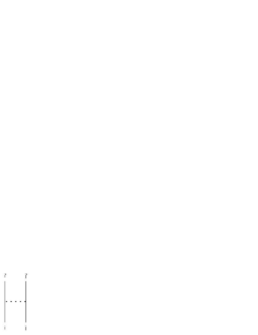
Figure 1: One-loop electromagnetic corrections to the baryon mass due to the Coulomb interaction between quarks. Note that the “quarks” represent spin-flavor index sets on baryon fields (not dynamical QCD quarks) and that spectator quarks are suppressed.

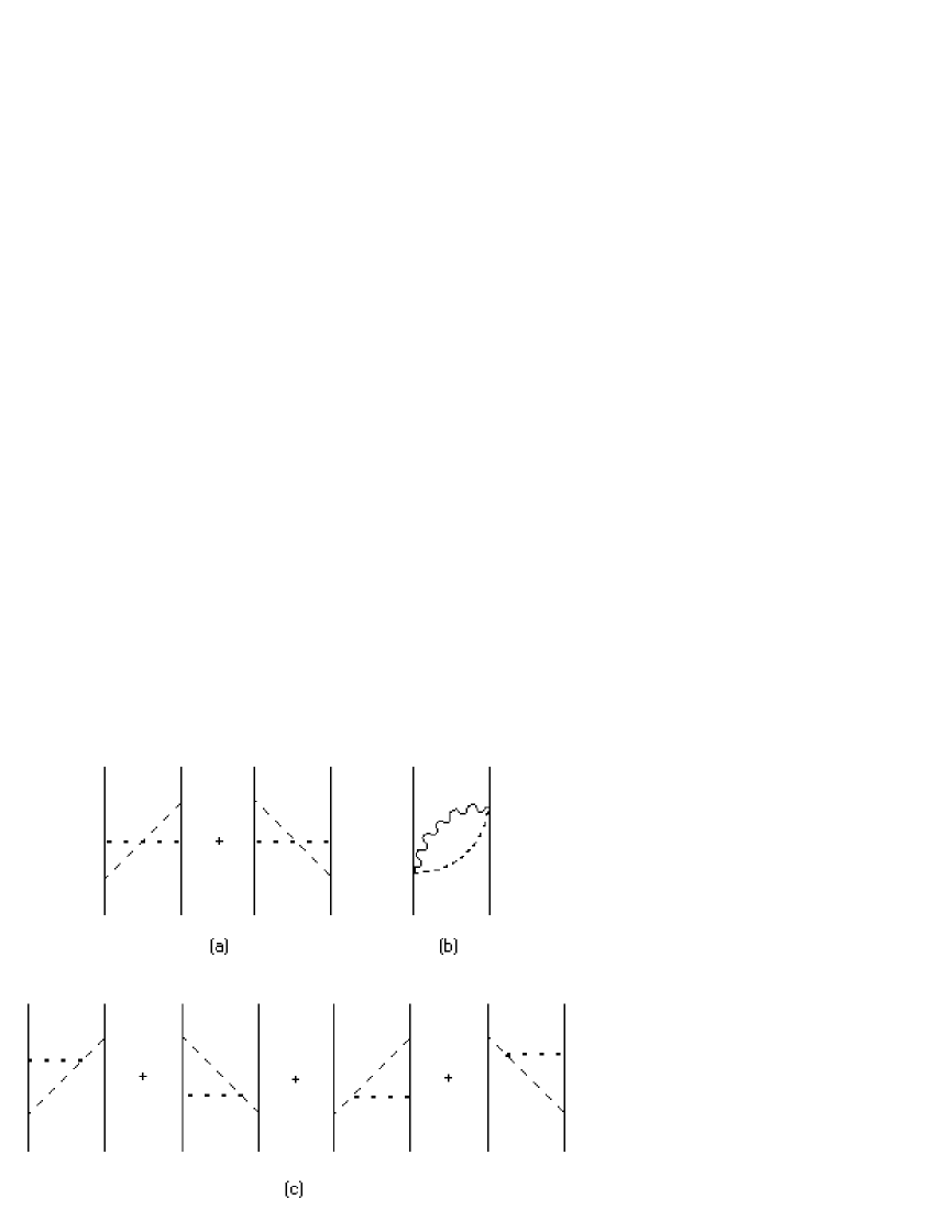
Figure 2: Two-loop corrections to electromagnetic interactions that involve meson exchange between quarks.

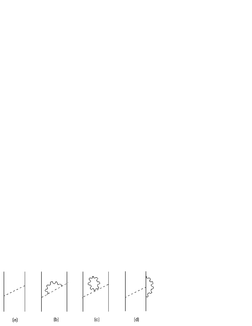
Figure 3: (a): The basic meson exchange diagram. (b), (c): Electromagnetic contributions to the meson mass terms. (d): electromagnetic correction to the meson-quark vertex.

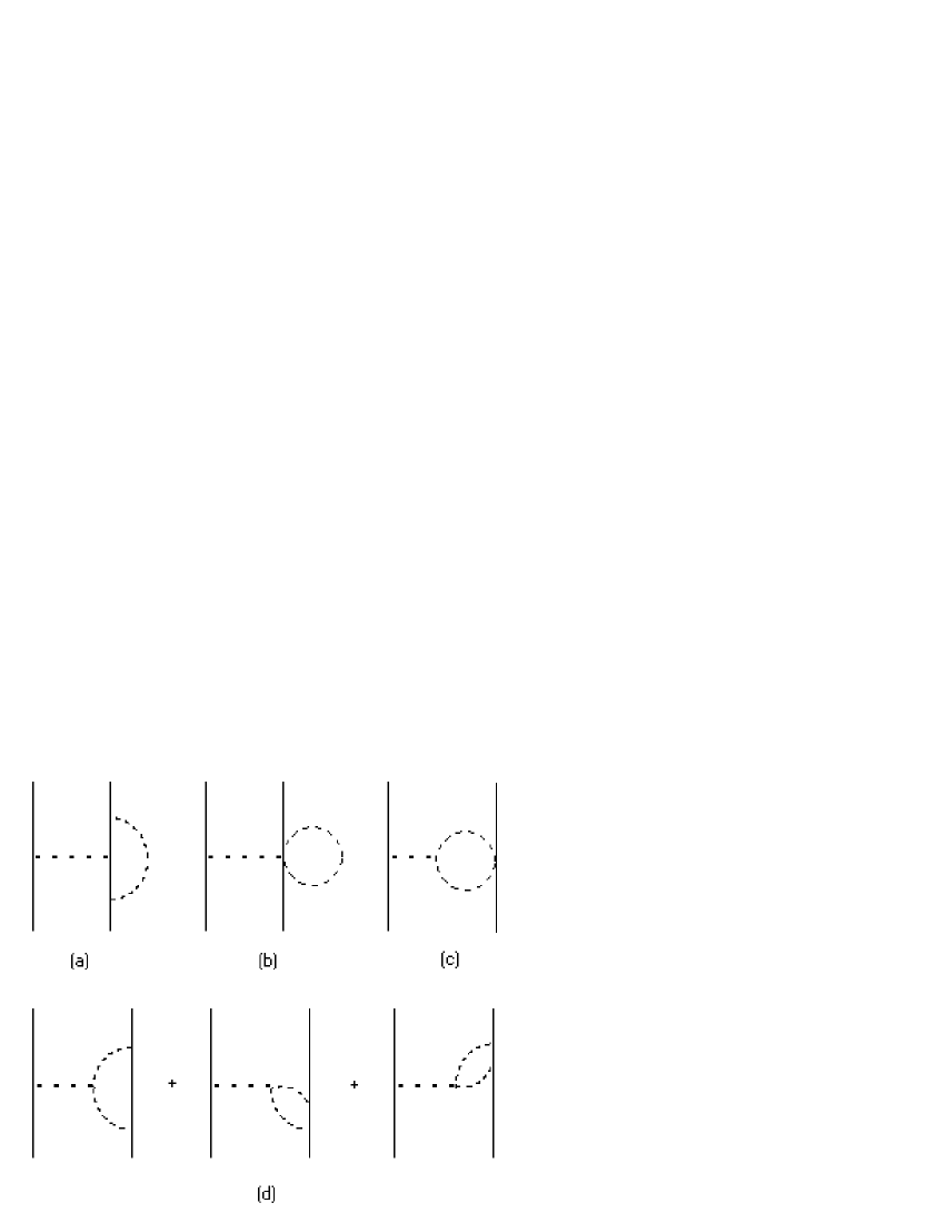
Figure 4: Mesonic corrections to electromagnetic vertices.

The second term in Eq. (13), $\mathcal{H}_{2}$, is the total contribution to the baryon mass differences from magnetic moment interactions

$$\mathcal{H}_{2} = -I_{\mu\mu}(\mu_{a}^{2}\Gamma_{5}+2\mu_{a}\mu_{b}\Gamma_{14})+\mathcal{H}^{\prime}_{9}+\mathcal{H}^{\prime}_{10}$$ (16)

$$+\frac{2}{9}\left[\mu_{a}(9\mu_{a}+\mu_{b})I_{9,\pi}-2\mu_{a}(\mu_{a}+\mu_{b})\left(I_{9,\pi}-I_{9,K}\right)\right]\sum_{i}M^{d}_{i},$$

where

$$\mathcal{H}^{\prime}_{9} = -\frac{2}{3}\mu_{a}^{2}I_{9,\pi}(\Gamma_{2}+3\Gamma_{4})+6\mu_{a}^{2}(I_{9,\pi}-\frac{4}{27}I_{9,\eta})\Gamma_{5}$$ (17)

$$+\frac{2}{3}\mu_{a}^{2}(I_{9,\pi}-I_{9,K})(9\Gamma_{10}+\Gamma_{11})+4\mu_{a}\left[\mu_{a}I_{9,\pi}-(\mu_{a}+\mu_{b})I_{9,K}\right]\Gamma_{13}$$

$$+\frac{4}{3}\mu_{a}\left[-9\mu_{a}I_{9,\pi}+5(\mu_{a}+\mu_{b})I_{9,K}+\frac{4}{3}(3\mu_{a}+2\mu_{b})I_{9,\eta}\right]\Gamma_{14}\ ,$$

and

$$\mathcal{H}^{\prime}_{10} = \frac{4}{3}\mu_{a}^{2}\,(4I_{9,\pi}+3I_{9,K}+\frac{2}{3}I_{9,\eta})\,\Gamma_{5}$$ (18)

$$+\frac{4}{3}\mu_{a}\left[(5\mu_{b}-3\mu_{a})I_{9,\pi}+(\mu_{a}+7\mu_{b})I_{9,K}+2(\mu_{a}+\frac{5}{3}\mu_{b})I_{9,\eta}\right]\,\Gamma_{14}\ .$$

Here, $\mu_{a}=2.793$ , $\mu_{b}=-0.933$; $I_{\mu\mu}$ and $I_{9,l}$ are the integrals associated with the direct interaction between magnetic moments (Fig. 5(a)) and the moment-moment interaction including one-loop mesonic corrections (Figs. 5(b) and 5(c)), respectively.

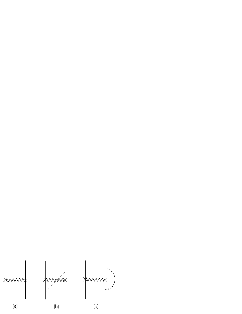
Figure 5: Instantaneous magnetic moment-moment interactions and mesonic corrections. A zigzag line with crosses at the vertices represents a factor $\mathcal{H}_{\mu\mu}\equiv-\mu_{i}\mu_{j}\bm{\sigma}_{i}\cdot\bm{\sigma}_{j}\,I_{\mu\mu}$

The third term in Eq. (13), $\mathcal{H}_{3}$, involving the effects of the $d,\,u$ quark mass differences on the baryon masses and on the single meson exchange amplitude, is of the form

$$\mathcal{H}_{3}=\Delta_{du}\sum_{i}M^{d}_{i}+\frac{2\Delta^{M}_{q}}{3\Delta^{M}_{\textrm{em}}}I_{4,K^{0}}\,\left[12\Gamma_{13}-6\Gamma_{10}-4\Gamma_{14}+2\Gamma_{11}\right]\,,$$ (19)

where $\Delta^{M}_{q}\equiv M_{K^{0}}^{2}-M_{K^{\pm}}^{2}+\Delta^{M}_{\textrm{em}}$, $\Delta^{M}_{\textrm{em}}=M_{\pi^{\pm}}^{2}-M_{\pi^{0}}^{2}$, and $\Delta_{du}=[(m_{d}-m_{u})/(m_{s}-m_{u})]\tilde{\alpha}_{m}$ is originally the coefficient of $\sum_{i}M^{d}_{i}$ from the single-particle mass operator at the quark level . Using the value $\tilde{\alpha}_{m}\approx 178$ MeV obtained in the absence of loop corrections Durand et al. (2002); Ha and Durand (1999) and the ratio $(m_{d}-m_{u})/(m_{s}-m_{u})\approx 0.227$ Weinberg (1996) gives the estimate $\Delta_{du}\approx 4.04$ MeV. Here, we will take into account the possible loop corrections to $\tilde{\alpha}_{m}$ and will treat $\Delta_{du}$ as a parameter.

The operators $\Gamma_{i}$ that appear above are all independent. However, contributions of their matrix elements to intramultiplet mass splittings satisfy a number of relations with $\Gamma_{10}=-\Gamma_{13}$, $\Gamma_{11}=-\Gamma_{14}=\Gamma_{10}+\frac{1}{2}(\Gamma_{4}-\Gamma_{5})$, and $\Gamma_{2}=-\frac{1}{3}\sum_{i}M^{d}_{i}+\frac{1}{2}(\Gamma_{4}-\Gamma_{5})$. Note also that $\Gamma_{19}=\Gamma_{20}$ and $\Gamma_{25}=\Gamma_{26}$ do not contribute. We can therefore bring $\mathcal{H}_{j}$, $(j=1,2,3)$ to a form similar to Eq. (1)

$$\mathcal{H}_{j}=a_{j}\sum_{i}M^{d}_{i}+b_{j}\Gamma_{4}+c_{j}\Gamma_{5}+d_{j}\Gamma_{13}\,,$$ (20)

where the coefficients of $\mathcal{H}_{1}$ are

$$a_{1} = \frac{4}{3}[\mathcal{I}_{1,\pi}-2(\mathcal{I}_{2,\pi}-\mathcal{I}_{2,K})]\,,$$

$$b_{1} = I_{QQ}+4\mathcal{I}_{1,\pi}+3\mathcal{I}_{1,K}-8(2\mathcal{I}_{2,\pi}+\mathcal{I}_{2,K})\,,$$

$$c_{1} = -3\mathcal{I}_{1,K}\,,$$ (21)

$$d_{1} = 12[-(\mathcal{I}_{1,\pi}-\mathcal{I}_{1,K})+2(\mathcal{I}_{2,\pi}-\mathcal{I}_{2,K})]\,,$$

the coefficients of $\mathcal{H}_{2}$ are

$$a_{2} = \frac{2}{9}\mu_{a}\left[(8\mu_{a}-\mu_{b})I_{9,\pi}+2(\mu_{a}+\mu_{b})I_{9,K}\right]\,,$$

$$b_{2} = \mu_{a}\mu_{b}I_{\mu\mu}+\frac{1}{3}\mu_{a}\left[(18\mu_{a}-10\mu_{b})I_{9,\pi}-(13\mu_{a}+24\mu_{b})I_{9,K}-12(\mu_{a}+\mu_{b})I_{9,\eta}\right]\,,$$

$$c_{2} = -\mu_{a}(\mu_{a}+\mu_{b})I_{\mu\mu}+\frac{1}{3}\mu_{a}\left[10(\mu_{a}+\mu_{b})I_{9,\pi}+(25\mu_{a}+24\mu_{b})I_{9,K}+12(\mu_{a}+\mu_{b})I_{9,\eta}\right]\,,$$ (22)

$$d_{2} = -2\mu_{a}\mu_{b}I_{\mu\mu}+\frac{4}{3}\mu_{a}\left[(5\mu_{b}-14\mu_{a})I_{9,\pi}+(8\mu_{a}+9\mu_{b})I_{9,K}+6(\mu_{a}+\mu_{b})I_{9,\eta}\right]\,,$$

and, finally, the coefficients of $\mathcal{H}_{3}$ are

$$a_{3}=\Delta_{du}\,,\ \ b_{3}=2(\Delta^{M}_{q}/\Delta^{M}_{\textrm{em}})I_{4,K^{0}}\,,\ \ c_{3}=-2(\Delta^{M}_{q}/\Delta^{M}_{\textrm{em}})I_{4,K^{0}}\,,\ \ d_{3}=8(\Delta^{M}_{q}/\Delta^{M}_{\textrm{em}})I_{4,K^{0}}\,.$$ (23)

It follows from Eqs. (1), (13), and (20) that

$$a=\sum_{i=1}^{3}a_{i}+a_{\textrm{CM}}\,,\ \ b=\sum_{i=1}^{3}b_{i}+b_{\textrm{CM}}\,,\ \ c=\sum_{i=1}^{3}c_{i}+c_{\textrm{CM}}\,,\ \ d=\sum_{i=1}^{3}d_{i}+d_{\textrm{CM}}\,.$$ (24)

The coefficients $a_{\textrm{CM}}$, $b_{\textrm{CM}}$, $c_{\textrm{CM}}$, and $d_{\textrm{CM}}$ are defined by Eq. (10).

In the next section, we will first evaluate the integrals and then study how well the dynamical theory developed in our earlier analyses of the baryon masses and magnetic moments describes the coefficients in $\mathcal{H}_{\textrm{IB}}$.

III The integrals

Let us start with the Coulomb integral $I_{QQ}$ and the magnetic integral $I_{\mu\mu}$ defined as

$$I_{QQ}=e^{2}\int\frac{d^{3}k}{(2\pi)^{3}|\bm{k}|^{2}}\,,\,\,\,I_{\mu\mu}=\frac{2\mu_{N}^{2}}{3}\int\frac{d^{3}k}{(2\pi)^{3}}\,,$$ (25)

where $\mu_{N}=e/(2m_{N})$ is the nucleon magneton.

Note that Eq. (25) refers only to the “bare” Coulomb and magnetic interactions between quarks without effects of baryon structure. These integrals and others to follow are formally divergent. The divergences are commonly absorbed in the HBA to chiral effective field theory into unknown constants representing short-distance effects that are to be evaluated from experiment.

In dynamical models, the integrals arise from matrix elements of the corresponding operators in physical baryon states, and those matrix elements involve additional momentum-dependent factors associated with the structure of the baryon which may regularize the integrals . Our objective here is to estimate the soft or long-distance contributions to the integrals, and to see the extent to which these account for the magnitude and pattern of baryon mass splittings. We therefore adopt the dynamical approach. This requires information on the internal structure of the baryons, some of which is available through measured baryon form factors and the semirelativistic theory of baryon structure, but its use necessarily involves models that go beyond the HBA to chiral effective field theory.

The semirelativistic theory of baryon structure has been considered by a number of authors and is quite successful Brambilla et al. (1994); Carlson et al. (1983); Capstick and Isgur (1986). For simplicity, we will use the model considered in Ha and Durand (2003) in which the baryon masses are calculated variationally for the semirelativistic Hamiltonian of Brambilla et al. using Gaussian wave functions. The results agree with those of a similar calculation by Carlson, Kogut, and Pandharipande Carlson et al. (1983) and are consistent with those of the much more extensive calculations of Capstick and Isgur Capstick and Isgur (1986).

We will use Jacobi coordinates to describe the positions of the quarks. Define

$${\textbf{r}}_{ij} = \bm{x}_{i}-\bm{x}_{j}\,,\ \ {\bf R}_{ij}=\frac{m_{i}\bm{x}_{i}+m_{j}\bm{x}_{j}}{m_{ij}}\,,$$

$${\textbf{r}}_{ij,k} = {\bf R}_{ij}-\bm{x}_{k}\,=\,\frac{m_{i}(\bm{x}_{i}-\bm{x}_{k})+m_{j}(\bm{x}_{j}-\bm{x}_{k})}{m_{ij}}\,,$$

$${\bf R}_{ijk} = \frac{m_{ij}{\bf R}_{ij}+m_{k}\bm{x}_{k}}{M}\,,$$ (26)

where the $\bm{x}_{i}$ are the particle coordinates, $m_{ij}=m_{i}+m_{j}$, $M=m_{i}+m_{j}+m_{k}$, and ${\bf R}_{ijk}$ is the usual center-of-mass coordinate. The roles of $i$, $j$, and $k$ are completely symmetric at this stage. However, it is reasonable to neglect the very small difference between the effective masses of the $u$ and $d$ quarks in the dynamical calculations. At least two of the quarks in each baryon are then identical or have the same mass. We label these 1 and 2, with the odd quark labelled 3 and then define the internal Jacobi coordinates $\bm{\rho}$ and $\bm{\lambda}$ as $\bm{\rho}={\textbf{r}}_{12}$ and $\bm{\lambda}={\textbf{r}}_{12,3}$. Alternatively, we can use coordinates with the role of $(1,2)$ replaced by $(2,3)$ or $(3,1)$ in the definition, and define $\bm{\rho}^{\prime}={\textbf{r}}_{23}$, $\bm{\lambda}^{\prime}={\textbf{r}}_{23,1}$, or $\bm{\rho}^{\prime\prime}={\textbf{r}}_{31}$, $\bm{\lambda}^{\prime\prime}={\textbf{r}}_{31,2}$. The coordinate pairs $\bm{\rho}^{\prime}$, $\bm{\lambda}^{\prime}$ and $\bm{\rho}^{\prime\prime}$, $\bm{\lambda}^{\prime\prime}$ can be expressed in terms of $\bm{\rho}$ and $\bm{\lambda}$ and conversely, so one can work with whichever of the pairs is most convenient and switch between them as necessary. The spatial volume element is simply $d^{3}R\,d^{3}\rho\,d^{3}\lambda$, and is equivalent for the other pairs of internal coordinates.

In the position space, we can express $I_{QQ}$ and $I_{\mu\mu}$, for the symmetrical case , as follows

$$I_{QQ}=\frac{e^{2}}{4\pi}\int d^{3}\rho\,d^{3}\lambda\,\frac{\left|\psi(\bm{\rho},\bm{\lambda})\right|^{2}}{\rho},\,\,\,I_{\mu\mu}=\frac{2\mu_{N}^{2}}{3}\int d^{3}\rho\,d^{3}\lambda\,\left|\psi(\bm{\rho},\bm{\lambda})\right|^{2}\delta^{3}(\bm{\rho})\ .$$ (27)

Using the position-space variational Gaussian wave functions in Ha and Durand (2003) for the $L=0$ ground states

$$\psi_{0}(\bm{\rho},\bm{\lambda})=\left(\frac{\beta_{\rho}\beta_{\lambda}}{\pi}\right)^{3/2}\exp{[-\frac{1}{2}(\beta_{\rho}^{2}\rho^{2}+\beta_{\lambda}^{2}\lambda^{2})]}\ ,$$ (28)

and changing coordinates appropriately Ha and Durand (2003), we can easily calculate $I_{QQ}$ and $I_{\mu\mu}$. The results are

$$I_{QQ}=\frac{2\alpha_{\textrm{em}}}{\sqrt{\pi}}\beta_{\rho},\,\,\,I_{\mu\mu}=\frac{2\mu_{N}^{2}}{3}\frac{\beta_{\rho}^{3}}{\sqrt{\pi^{3}}},$$ (29)

where $\alpha_{\textrm{em}}=e^{2}/4\pi$. For $\beta_{\rho}=340$ MeV obtained for the nucleon, $I_{QQ}=2.80\,\textrm{MeV}$ and $I_{\mu\mu}=0.123\,\textrm{MeV}$.

Next, we consider the integrals associated with the mesonic corrections.

$I_{1,l}$ comes from the diagram in Fig. 2(a) and, as shown in Durand and Ha (2005), factors into the product of a Coulomb integral and a mesonic integral $I_{1,l}^{\prime}$.

$$I_{1,l}=I_{QQ}\times I_{1,l}^{\prime}\,,\,\,\,I_{1,l}^{\prime}=\frac{\beta^{2}}{4f^{2}}\int\frac{d^{3}k^{\prime}}{(2\pi)^{3}2E_{l}^{\prime}}\frac{k^{{}^{\prime}2}}{E_{l}^{{}^{\prime}2}}F_{A}^{2}(\bm{k}^{{}^{\prime}2})\,,$$ (30)

where $\beta$ is a common dynamical matrix element for meson emission Durand et al. (2002) , $E_{l}(\bm{k}^{\prime})=\sqrt{\bm{k}^{{}^{\prime}2}+M_{l}^{2}}$, and $F_{A}(\bm{k}^{{}^{\prime}2})$ is the axial vector form factor of the baryon introduced when we neglect the excited states and include the internal structure of the baryon through the baryon wave function.

To evaluate the mesonic integral $I_{1,l}^{\prime}$, we use the dipole form factor $F_{A}(\bm{k}^{{}^{\prime}2})=\Lambda_{A}^{4}/(\Lambda_{A}^{2}+\bm{k}^{{}^{\prime}2})^{2}$ used in our earlier analyses of baryon masses Ha and Durand (1999); Durand et al. (2002). The mesonic integral $I_{1,l}^{\prime}$ is convergent and easy to be numerically calculated. For $\Lambda_{A}=850$ MeV and $\beta=0.75$, we find that $I_{1,\pi}^{\prime}=0.039$, $I_{1,K}^{\prime}=0.016$, and $I_{1,\eta}^{\prime}=0.014$.

$I_{2,l}$ comes from the diagram in Fig. 2(b) and is given by

$$I_{2,l}=\frac{e^{2}\beta^{2}}{f^{2}}\int\frac{d^{3}k}{(2\pi)^{3}|\bm{k}|}\int\frac{d^{3}k^{\prime}}{(2\pi)^{3}2E^{\prime}_{l}}\frac{1}{E+E^{\prime}_{l}}(F_{Q}(\bm{k}^{2})F_{A}(\bm{k}^{{}^{\prime}2}))^{2}\,.$$ (31)

Note that a product of the form factors, $F_{Q}(\bm{k}^{2})F_{A}(\bm{k}^{{}^{\prime}2})$ is introduced at each vertex of the diagram to ensure that $I_{2,l}$ is convergent. To evaluate the integral numerically, we use a nucleon form factor $F_{Q}(\bm{k}^{2})=\Lambda_{Q}^{4}/(\Lambda_{Q}^{2}+\bm{k}^{2})^{2}$ with $\Lambda_{Q}=843$ MeV Hyde-Wright and de Jager (2004).

$I_{3,l}$ comes from the diagram in Fig. 2(c) whose intermediate matrix element, showing all quarks, is like a baryon-meson scattering matrix element. We will introduce a product of charge form factors $F_{Q}(\bm{k}^{2})F_{M}(\bm{k}^{2})$ to the intermediate state where $F_{M}(\bm{k}^{2})=\Lambda_{M}^{4}/(\Lambda_{M}^{2}+\bm{k}^{2})^{2}$ is the meson charge form factor with $\Lambda_{M}=1017$ MeV. Hence,

$$I_{3,l}=\frac{e^{2}\beta^{2}}{4f^{2}}\int\frac{d^{3}k}{(2\pi)^{3}|\bm{k}|^{2}}F_{Q}(\bm{k}^{2})F_{M}(\bm{k}^{2})\int\frac{d^{3}k^{\prime}}{(2\pi)^{3}}\frac{\bm{k}^{\prime}\cdot\bm{k}^{\prime\prime}}{4E_{l}^{\prime}E_{l}^{\prime\prime}}\frac{E_{l}^{\prime}+E_{l}^{\prime\prime}}{E_{l}^{\prime}E_{l}^{\prime\prime}}F_{A}(\bm{k}^{{}^{\prime}2})F_{A}(\bm{k}^{{}^{\prime\prime}2})\,,$$ (32)

where $\bm{k}^{\prime\prime}=\bm{k}^{\prime}+\bm{k}$ .

$I_{4,l}$ comes from the diagram in Fig. 3(a) differentiated with respect to $M_{l}^{2}$. It is defined as

$$I_{4,l}=\frac{\beta^{2}\Delta^{M}_{\textrm{em}}}{4f^{2}}\int\frac{d^{3}k^{\prime}}{(2\pi)^{3}2E_{l}^{\prime}}\frac{k^{{}^{\prime}2}}{E_{l}^{\prime 3}}F_{A}^{2}(\bm{k}^{{}^{\prime}2})\,.$$ (33)

This integral can be analytically evaluated. The result is

$$I_{4,l}=\frac{\beta^{2}\Delta^{M}_{\textrm{em}}}{512\pi f^{2}}\frac{\lambda_{A}^{5}(M_{l}+5\lambda_{A})}{(M_{l}+\lambda_{A})^{5}}\,.$$ (34)

$I_{5,l}$ is the integral associated with the diagram in Fig. 4(a) and is identical to $I_{1,l}$, i.e., $I_{5,l}=I_{1,l}$.

$I_{6,l}$ comes from the diagram in Fig. 4(b). The extended structure at the vertex in Fig. 4(b) suggests that the same form factor as in Fig. 4(a) should be used. For the rest of the diagram, a Coulomb interaction must be absorbed by the wave function (not the form factor). So, for the symmetrical case, we get

$$I_{6,l}=\frac{e^{2}\beta^{2}}{4f^{2}}\int\frac{d^{3}k}{(2\pi)^{3}|\bm{k}|^{2}}\int d^{3}\lambda\,\left|\tilde{\psi}(\bm{k},\bm{\lambda})\right|^{2}\int\frac{d^{3}k^{\prime}}{(2\pi)^{3}2E^{\prime}_{l}}F_{A}^{2}(\bm{k}^{{}^{\prime}2})\,,$$ (35)

where

$$\left|\tilde{\psi}(\bm{k},\bm{\lambda})\right|^{2}=\int d^{3}\rho\ e^{-i\bm{k}\cdot\bm{\rho}}\left|\psi(\bm{\rho},\bm{\lambda})\right|^{2}\,.$$ (36)

Using the Gaussian wave functions, Eq. (28), we find

$$\int d^{3}\lambda\,\left|\tilde{\psi}(\bm{k},\bm{\lambda})\right|^{2}=\exp[-k^{2}/(4\beta_{\rho}^{2})]\,,\,\,\,I_{QQ}=e^{2}\int\frac{d^{3}k}{(2\pi)^{3}|\bm{k}|^{2}}e^{-k^{2}/(4\beta_{\rho}^{2})}\,.$$ (37)

Hence,

$$I_{6,l}=I_{QQ}\times\frac{\beta^{2}}{4f^{2}}\int\frac{d^{3}k^{\prime}}{(2\pi)^{3}2E_{l}^{\prime}}F_{A}^{2}(\bm{k}^{{}^{\prime}2})\ .$$ (38)

$I_{7,l}$ and $I_{8,l}$ come from the diagrams in Figs. 4(c) and 4(d), respectively. The intermediate state of the diagram in Fig. 4(d) has the baryon-meson scattering structure, thus it involves $F_{Q}(\bm{k}^{2})F_{M}(\bm{k}^{2})$. The diagram in Fig. 4(c) is related to the one in Fig. 4(d). Its intermediate part involves the baryon-meson scattering structure contracted with a meson-meson-baryon vertex but instantaneous, not scattering. Putting in the form factors,

$$I_{7,l}=\frac{e^{2}\beta^{2}}{4f^{2}}\int\frac{d^{3}k}{(2\pi)^{3}|\bm{k}|^{2}}\int d^{3}\lambda\,\left|\tilde{\psi}(\bm{k},\bm{\lambda})\right|^{2}\int\frac{d^{3}k^{\prime}}{(2\pi)^{3}}\frac{1}{E^{\prime}_{l}+E^{\prime\prime}_{l}}F_{A}(\bm{k}^{{}^{\prime}2})F_{A}(\bm{k}^{{}^{\prime\prime}2})\,,$$ (39)

and

$$I_{8,l}=\frac{e^{2}\beta^{2}}{4f^{2}}\int\frac{d^{3}k}{(2\pi)^{3}|\bm{k}|^{2}}F_{Q}(\bm{k}^{2})F_{M}(\bm{k}^{2})\int\frac{d^{3}k^{\prime}}{(2\pi)^{3}}\frac{\bm{k}^{\prime}\cdot\bm{k}^{\prime\prime}}{E_{l}^{\prime}E_{l}^{\prime\prime}}\frac{1}{E_{l}^{\prime}+E_{l}^{\prime\prime}}F_{A}(\bm{k}^{{}^{\prime}2})F_{A}(\bm{k}^{{}^{\prime\prime}2})\,.$$ (40)

At this point, it is important to note that the diagrams in Fig. 4 are related by electromagnetic current conservation. The sum of these diagrams associated with mesonic corrections to the photon-quark vertex must give a coefficient for the $1/\bm{k}^{2}$ Coulomb singularity that vanishes in the limit of zero photon momentum, $\bm{k}\rightarrow 0$. This condition is found to hold for the diagrams without form factors Durand and Ha (2005). It is straightforward to check that the condition still hold for the diagrams with wave functions and form factors. Indeed, since the integrals $I_{6,l}$ and $I_{7,l}$ appear with opposite-sign coefficients and for $\bm{k}\rightarrow 0$ the integral over $\lambda$ in their expressions is just the normalization integral and hence approaches unity, the coefficient of $1/\bm{k}^{2}$ vanishes when $I_{6,l}$ and $I_{7,l}$ are combined. Similarly, we can easily show the cancellation between the $I_{5,l}$ and $I_{8,l}$ terms for $\bm{k}\rightarrow 0$ if we write $I_{5,l}$ explicitly and notice that the form factors in the first factor in $I_{8,l}$ also approach unity for $\bm{k}\rightarrow 0$.

Finally, $I_{9,l}$ and $I_{10,l}$ come from Figs. 5(b) and 5(c), respectively. They are identical and factor into the product of $I_{\mu\mu}$ and the mesonic integral $I_{1,l}^{\prime}$

$$I_{9,l}=I_{10,l}=I_{\mu\mu}\times I_{1,l}^{\prime}\,.$$ (41)

It is straightforward to evaluate $I_{1,l}$,$I_{2,l}$,$I_{6,l}$, and $I_{9,l}$ numerically. To evaluate $I_{3,l}$, $I_{7,l}$, and $I_{8,l}$, we integrate first on $d\Omega_{k^{\prime}}$ with the polar axis chosen along $\bm{k}$. The obtained results are then integrated numerically.

We present in Table 2 the numerical values of $I_{i}$ $(i=1,...,9)$, $\mathcal{I}_{1}$, and $\mathcal{I}_{2}$ for different meson loops. All the integrals are measured in MeV. Calculations use $\alpha_{\textrm{em}}=1/137$, $f\approx 93.0$ MeV, $\beta=0.75$, $\lambda_{A}=850$ MeV, $\lambda_{Q}=843$ MeV, $\lambda_{M}=1017$ MeV, and $\beta_{\rho}=340$ MeV.

Table 2: Numerical values of $I_{i}$ $(i=1,...,9)$, $\mathcal{I}_{1}$, and $\mathcal{I}_{2}$ for different meson loops. All the integrals are measured in MeV. Calculations use $\alpha_{\textrm{em}}=1/137$, $f\approx 93.0$ MeV, $\beta=0.75$, $\lambda_{A}=850$ MeV, $\lambda_{Q}=843$ MeV, $\lambda_{M}=1017$ MeV, $\beta_{\rho}=340$ MeV.

Integral	$\pi$-meson	K-meson	$\eta$-meson
$I_{1}$	0.108	0.045	0.040
$I_{2}$	0.113	0.058	0.053
$I_{3}$	0.059	0.027	0.024
$I_{4}$	0.105	0.024	0.020
$I_{5}$	0.108	0.045	0.040
$I_{6}$	0.126	0.087	0.082
$I_{7}$	0.100	0.073	0.069
$I_{8}$	0.057	0.027	0.024
$I_{9}$	0.005	0.002	0.002
$\mathcal{I}_{1}$	0.008	0.025	0.024
$\mathcal{I}_{2}$	0.038	0.016	0.014

Since our loop calculations involve divergent integrals, cutoff-dependence of the results is inevitable. To explore this point further, we also estimate the integrals using a monopole form for the meson form factors suggested by the vector dominance model O’Connell et al. (1997). The cut-off parameters $\lambda$’s for the monopole form factors are chosen such that the mean square radii determined by the two forms (monopole and dipole) are the same. We show in Table 3 the numerical values of $I_{i}$ $(i=1,...,9)$, $\mathcal{I}_{1}$, and $\mathcal{I}_{2}$ for different meson loops for case of using monopole form factors. All the integrals are measured in MeV. Calculations use $\lambda_{A}=601$ MeV, $\lambda_{Q}=596$ MeV, $\lambda_{M}=719$ MeV, $\alpha_{\textrm{em}}=1/137$, $f\approx 93.0$ MeV, $\beta=0.75$, and $\beta_{\rho}=340$ MeV.

Table 3: Numerical values of $I_{i}$ $(i=1,...,9)$, $\mathcal{I}_{1}$, and $\mathcal{I}_{2}$ for different meson loops when using monopole form factors. All the integrals are measured in MeV. Calculations use $\alpha_{\textrm{em}}=1/137$, $f\approx 93.0$ MeV, $\beta=0.75$, $\beta_{\rho}=340$ MeV, $\lambda_{A}=601$ MeV, $\lambda_{Q}=596$ MeV, and $\lambda_{M}=719$ MeV.

Integral	$\pi$-meson	K-meson	$\eta$-meson
$I_{1}$	0.176	0.097	0.090
$I_{2}$	0.185	0.110	0.102
$I_{3}$	0.113	0.069	0.065
$I_{4}$	0.132	0.041	0.035
$I_{5}$	0.176	0.097	0.090
$I_{6}$	0.194	0.149	0.144
$I_{7}$	0.168	0.135	0.131
$I_{8}$	0.111	0.069	0.064
$I_{9}$	0.008	0.004	0.004
$\mathcal{I}_{1}$	0.052	0.060	0.058
$\mathcal{I}_{2}$	0.045	0.021	0.020

IV The coefficients $a$, $b$, $c$, and $d$

To evaluate the coefficients $a$, $b$, $c$, and $d$, we first need to estimate the coefficients $a_{\textrm{CM}}$, $b_{\textrm{CM}}$, $c_{\textrm{CM}}$, and $d_{\textrm{CM}}$ given by Eq. (10). Using $m_{u}\approx 340$ MeV, $(m_{d}-m_{u})\approx 2.5$ MeV, $(m_{d}-m_{u})/m_{u}=0.0074\pm 0.0012$, and a result from the simple quark model

$$6\frac{4\pi\alpha_{s}}{9}A=m_{\Delta}-m_{N}\approx 300\,{\textrm{MeV}}\,,$$ (42)

we get $C=0.37\pm 0.06$ MeV. Thus, for $m_{s}\approx 500$ MeV, the color-magnetic contributions to the four parameters $a$, $b$, $c$, and $d$ (in MeV) are

$$a_{\textrm{CM}}=-0.74\pm 0.12,\,\,b_{\textrm{CM}}=0.75\pm 0.12,\,\,c_{\textrm{CM}}=-0.75\pm 0.12,\,\,d_{\textrm{CM}}=0.70\pm 0.44\,.$$ (43)

Next, using $\Delta^{M}_{\textrm{em}}=1260$ ${\textrm{MeV}}^{2}$, $\Delta^{M}_{q}=5196$ ${\textrm{MeV}}^{2}$, and the values of the integrals given in Table 2 (Table 3 for the case of using monopole form factors), it is straightforward to calculate numerically the coefficients $b$, $c$, and $d$. To evaluate the coefficient $a$, we have used $\Delta_{du}$ as a parameter and fitted $a$ exactly to its experimental value. A best fit is obtained at $\Delta_{du}=2.54\pm 0.00$ MeV ($\Delta_{du}=2.43\pm 0.00$ MeV when using monopole form factors), a value that is lower than the value $\Delta_{du}\approx 4.04$ MeV estimated ignoring loop corrections to $\tilde{\alpha}_{m}$ . The calculated values of the coefficients $a$, $b$, $c$, and $d$ (in MeV) are

$$a=1.82\pm 0.12,\,\,b=3.00\pm 0.12,\,\,c=-1.46\pm 0.12,\,\,d=2.28\pm 0.44\,,$$ (44)

for the case of using dipole form factors, and

$$a=1.82\pm 0.12,\,\,b=3.34\pm 0.12,\,\,c=-1.50\pm 0.12,\,\,d=2.48\pm 0.44\,,$$ (45)

for the case of using monopole form factors.

The calculated values of $a$, $b$, $c$, and $d$ for $\mathcal{H}_{\textrm{IB}}$ and the contributions to those values from $\mathcal{H}_{1}$, $\mathcal{H}_{2}$, $\mathcal{H}_{3}$, and $\mathcal{H}_{\textrm{CM}}$ for these two cases are shown in Table 4. The best fit values of the parameters from $\mathcal{H}_{\textrm{IB}}^{\textrm{best}}$ are also given there.

Table 4: Coefficients $a$, $b$, $c$, and $d$ from $\mathcal{H}_{1}$, $\mathcal{H}_{2}$, $\mathcal{H}_{3}$, $\mathcal{H}_{\textrm{CM}}$, $\mathcal{H}_{\textrm{IB}}$, and $\mathcal{H}_{\textrm{IB}}^{\textrm{best}}$. All values of the coefficients are in MeV. Calculations use $\Delta_{em}^{M}=1260$ ${\textrm{MeV}}^{2}$, $\Delta_{q}^{M}=5196$ ${\textrm{MeV}}^{2}$, the calculated values of the color-magnetic parameters given in Eq. (43), $\Delta_{du}=2.54\pm 0.00$ MeV obtained from a fit, and the values of the integrals shown in Table 2 ($\Delta_{du}=2.43\pm 0.00$ MeV and Table 3 for the case of using monopole form factors). The uncertainties shown for the theoretical values of the coefficients include only those from the uncertainties in the color-magnetic terms.

Hamiltonian	Dipole case				Monopole case
	$a$	$b$	$c$	$d$	$a$	$b$	$c$	$d$
$\mathcal{H}_{1}$	$-$0.05	2.17	$-$0.08	0.74	0.01	2.29	$-$0.18	0.67
$\mathcal{H}_{2}$	0.07	$-$0.12	$-$0.43	0.04	0.12	$-$0.03	$-$0.23	$-$0.23
$\mathcal{H}_{3}$	2.54	0.20	$-$0.20	0.80	2.43	0.33	$-$0.33	1.34
$\mathcal{H}_{\textrm{CM}}$	$-$0.74	0.75	$-$0.75	0.70	$-$0.74	0.75	$-$0.75	0.70
$\mathcal{H}_{\textrm{IB}}$	1.82 $\pm$ 0.12	3.00 $\pm$ 0.12	$-$1.46 $\pm$ 0.12	2.28 $\pm$ 0.44	1.82 $\pm$ 0.12	3.34 $\pm$ 0.12	$-$1.50 $\pm$ 0.12	2.48 $\pm$ 0.44
$\mathcal{H}_{\textrm{IB}}^{\textrm{best}}$	1.82 $\pm$ 0.04	3.35 $\pm$ 0.24	$-$1.78 $\pm$ 0.23	1.00 $\pm$ 1.40	1.82 $\pm$ 0.04	3.35 $\pm$ 0.24	$-$1.78 $\pm$ 0.23	1.00 $\pm$ 1.40

The results given in Table  4 show that the calculated IB corrections are of the right general size and have the correct sign pattern. These corrections seem to account fairly well for the pattern of coefficients $a$, $b$, $c$ in the IB mass-difference Hamiltonian. The coefficient $d$ has the correct sign, but its calculated magnitude appears to be somewhat large. However, like the other calculated values of $a$, $b$, and $c$, the calculated value of $d$ agrees with its experimental value within the margin of error. Using the values of $a$, $b$, $c$, and $d$ given in Eq. (44) for the dipole case, we can easily evaluate the baryon mass splittings shown in Eq. (II.2) and find that the average deviation of the calculated values from experiment is $0.23$ MeV with a weighted $\chi^{2}/n_{f}$ of $1.63$ for $n_{f}=3$ degrees of freedom ($p\approx 0.2$).

Note that employing a monopole form for the meson form factors improve the results for the coefficients $b$ and $c$, but not for $d$. Nevertheless, the calculated value of $d$ still agrees with its experimental value within the margin of error. Using the values $a$, $b$, $c$, and $d$ given in Eq. (45) for the monopole case, we find the average deviation of the calculated values from experiment to be $0.29$ MeV with a weighted $\chi^{2}/n_{f}=0.86$ for $n_{f}=3$ degrees of freedom ($p\approx 0.36$). The weighted fit is clearly better even though the average deviation is larger, the result of the uncertainty in the experimental value of $d$.

Since most of the integrals clearly have potentially large short-distance contributions (the divergences in the absence of form factors are strong), the presence of the short-distance effects is likely the source of any deviations from the experiment results. We do not regard the distinction between the dipole and monopole fits as definitive given the different short-distance behavior of the corresponding integrals.

To illustrate the uncertainty within the model, we note that if one supposes that the quark wave functions are exponential at short distances rather than Gaussian, $\exp{(-r/a)}$ rather than $\exp{(-\beta_{\rho}^{2}r^{2}/2)}$, but keep the dependence on $\lambda$ and the mean square separation $<r^{2}>$ the same, then $a=1/(\sqrt{2}\beta_{\rho})$ and the Coulomb integrals increase by $\sqrt{\pi/2}$. That is, the Coulomb integrals are underestimated using Gaussian wave functions which neglect short distance correlations. The more complicated wave functions used by Carlson et al. Carlson et al. (1983) include correlations and indeed give a some what larger energy as noted in Durand and Ha (2005). The same remarks hold for the magnetic integral. The short distance effects are even stronger there: the magnetic integrals calculated using the exponential wave functions increase by a factor $2\sqrt{2\pi}$. Therefore, $I_{QQ}$ and $I_{\mu\mu}$ can be treated as parameters by multiplying their expressions defined in Eq. (29) with the scale factors. We find, however, that doing so does not substantially improve the results.

It is encouraging that the model, with all parameters except $\Delta_{du}$ fixed gives as an accurate account of the purely electromagnetic parameters $b$, $c$, $d$.

V Conclusion

Our results here consist of a numerical analysis of the IB contributions to the baryon masses which we analyzed recently using a loop expansion in the heavy baryon approximation to chiral effective field theory and methods developed in our earlier analyses of the baryon masses and magnetic moments. The leading IB corrections to the baryon masses come from the Coulomb interaction, magnetic moments interactions, the effects of the $d,\,u$ quark mass difference, and effective point interactions attributable to color-magnetic effects.

We have made reasonable estimates of the various integrals by introducing the known form factors and wave functions from successful semirelativistic models for the baryons and using the results to evaluate the parameters. We find that the resulting contributions to the IB corrections are of the right general size, have the correct sign pattern, and agree with the experimental values within the margin of error. We also find that employing monopole instead of dipole form factors slightly improve the results, but scaling the Coulomb or magnetic moment contributions, does not. To the extent to which effects of adding a second meson loop are small, a view supported by the smallness of the three-body violations of the sum rules, it appears likely that any deviations from the experiment can be attributed to the presence of short-distance effects which can be parametrized but not calculated in the effective field theory.

*

Appendix A One- and two-body operators

We present here sets of one- and two- body operators defined earlier in Morpurgo (1992); Durand and Ha (2005). In the case of $\textrm{O}(e^{2})$ contributions to the baryon masses, the $\Gamma$’s must be bilinear in the quark charge matrix $Q=\textrm{diag}\,(2/3,-1/3,-1/3)$ and can depend otherwise on the quark spin matrices $\bm{\sigma}$ and and flavors. Ignoring isospin breaking through the small $u$, $d$ mass difference and using the conventions that

$$\sum[i]\equiv\sum_{i},\quad\sum[ij]\equiv\frac{1}{2}\sum_{i\not=j},\quad\sum[ijk]\equiv\frac{1}{6}\sum_{i\not=j\not=k},$$ (46)

where $i,j,k\in u,d,s$ label the three quarks in a baryon, we can group the $\Gamma$’s into sets of one- and two-quark operators as follows:

One-body operators:

$$\Gamma_{1}=\sum[Q_{i}^{2}],\quad\Gamma_{7}=\sum[Q_{i}^{2}M^{s}_{i}].$$ (47)

Two-body operators:

$$\Gamma_{2}=\sum[Q_{i}^{2}(\bm{\sigma}_{i}\cdot\bm{\sigma}_{j})],\quad\Gamma_{4}=\sum[Q_{i}Q_{j}],\quad\Gamma_{5}=\sum[Q_{i}Q_{j}(\bm{\sigma}_{i}\cdot\bm{\sigma}_{j})],$$ (48)

$$\Gamma_{8}=\sum[Q_{i}^{2}M^{s}_{i}(\bm{\sigma}_{i}\cdot\bm{\sigma}_{j})],\quad\Gamma_{10}=\sum[Q_{i}^{2}M^{s}_{j}],\quad\Gamma_{11}=\sum[Q_{i}^{2}M^{s}_{j}(\bm{\sigma}_{i}\cdot\bm{\sigma}_{j})],$$ (49)

$$\Gamma_{13}=\sum[Q_{i}Q_{j}M^{s}_{i}],\quad\Gamma_{14}=\sum[Q_{i}Q_{j}M^{s}_{i}(\bm{\sigma}_{i}\cdot\bm{\sigma}_{j})],$$ (50)

$$\Gamma_{19}=\sum[Q_{i}^{2}M^{s}_{i}M^{s}_{j}],\quad\Gamma_{20}=\sum[Q_{i}^{2}M^{s}_{i}M^{s}_{j}(\bm{\sigma}_{i}\cdot\bm{\sigma}_{j})],$$ (51)

$$\Gamma_{25}=\sum[Q_{i}Q_{j}M^{s}_{i}M^{s}_{j}],\quad\Gamma_{26}=\sum[Q_{i}Q_{j}M^{s}_{i}M^{s}_{j}(\bm{\sigma}_{i}\cdot\bm{\sigma}_{j})]\,.$$ (52)