Magnetic Induced Axion Mass

Abstract

We study the effect of a uniform magnetic field on the dynamics of axions. In particular, we show that the Peccei-Quinn symmetry is explicitly broken by the presence of an external magnetic field. This breaking is induced by the non-conservation of the magnetic helicity and generates an electromagnetic contribution to the axion mass. We compute the magnetic axion mass in one loop approximation, with no restriction on the intensity of the magnetic field, and including thermal effects.

Keywords: Axions, Magnetic Fields

I I. Introduction

Axions are the pseudoscalar particles predicted by the Peccei and Quinn (PQ) mechanism PQ , a quite elegant attempt to explain the smallness of the CP-violation induced by the QCD Lagrangian (the so-called strong CP problem; for a review see, e.g., Ref. Kim ). They emerge as Pseudo-Goldstone Boson modes associated with the global axial PQ-symmetry $U(1)_{\rm PQ}$, spontaneously broken at the PQ-scale $f_{a}$. This last is also known as the PQ- or axion-constant, and characterizes all the axion phenomenology. More specifically the axion mass is given by the relation Kim

$$m_{\tiny{\rm QCD}}/\mbox{eV}\simeq 6.2\times 10^{6}\mbox{GeV}/f_{a},$$ (1)

(here QCD means that this is induced by interaction with gluons) while its interactions with fermions are measured by $g_{i}\sim m_{i}/f_{a}$, where $m_{i}$ represents the fermion mass (e.g. $m_{e},m_{N},...$ for electrons, nucleons, etc.). In addition, though chargeless, axions interact with photons through the electromagnetic anomaly:

$$\mathcal{L}_{a\gamma}=\frac{1}{4}\,g_{a\gamma}\,a\,F\widetilde{F},$$ (2)

where $F$ is the electromagnetic field, $\widetilde{F}^{\mu\nu}=(1/2)\,\varepsilon^{\mu\nu\alpha\beta}F_{\alpha\beta}$ its dual, and $g_{a\gamma}=\alpha_{\rm em}\xi/(2\pi f_{a})$. Here, $\alpha_{\rm em}$ is the electromagnetic fine structure constant and $\xi$ an order one, model dependent constant. Presently, the PQ-constant’s allowed range is rather narrow Raff : terrestrial experiments together with astrophysical and cosmological considerations have in fact excluded all the values of $f_{a}$ up to $10^{9}\,\mbox{GeV}$, and above $10^{12}\,\mbox{GeV}$.

Because of the axion-photon interaction term (2), the phenomenology of axions can be influenced by the presence of an external electromagnetic field. Probably, the most discussed result of this well studied interaction is the axion-photon conversion in an external magnetic field (see, e.g., Ref. Raff88 ), which presently seems the best way to detect axions by terrestrial experiments Sikivie .

Another interesting consequence of interaction (2) was discussed in Ref. Mikheev where it was shown that axions in a strong magnetic field undergo a finite mass shift. However, in that computation of the mass shift the temperature effects were not taken into account. This makes the result in Ref. Mikheev , though correct, not directly applicable to the axion phenomenology. In fact, since the axion-photon coupling is very small, the induced mass can be relevant for the axion phenomenology only in the case of very intense magnetic fields, which normally exist only at high temperatures. In this paper, we reconsider this effect accounting also for the thermal contribution. As we will show, the result given in Ref. Mikheev is a very good approximation only for temperatures well below the electron mass $T\ll m_{e}$. For higher temperatures and sufficiently intense magnetic fields the thermal corrections are relevant.

Interestingly, the resulting mass shift induced by the magnetic field is independent of the gluon dynamics and, therefore, does not vanish if the (QCD induced) axion mass (1) is set to zero. In other words, the external electromagnetic field itself is responsible for the breaking of the PQ-symmetry, playing a role similar to the gluon fields. We will discuss this point in Section 2 of this paper. We will show that the magnetic contribution is indeed due to a topological effect (just as for gluons) which is expected when the axion dynamics take place in an external magnetic field. Ultimately, we will associate this effect with the generation of magnetic helicity, whose important role in axion cosmology has already been pointed out (see Ref. noi2 ). This property makes the magnetic mass shift a true mass term. Therefore, the terminology “mass shift” is perhaps inappropriate. In the following, we will refer to this contribution as the magnetic induced axion mass $m_{B}$. It contributes to the total axion mass as

$$m^{2}=m_{\tiny{\rm QCD}}^{2}+m_{B}^{2},$$ (3)

where $m_{\tiny{\rm QCD}}$ is given in (1).

Because of this property, our result applies not only to axions but to any pseudoscalar particle which interacts with photons as in Eq. (2), independent of its interaction with gluons. This is the case with arions Anselm , (almost) massless pseudoscalar particles which do not interact with gluons at all. On the other hand, concerning the axion phenomenology, we expect the contribution $m_{B}$ to be especially relevant at temperatures above $\sim 1\mbox{GeV}$, where the gluon contribution to the axion mass is strongly suppressed GPY , or in regions of space and time where a very strong magnetic field is present. A more detailed analysis of the phenomenological implications of the magnetic induced axion mass is in progress.

The paper is organized as follows: In Section 2 we comment on the origin of the magnetic induced mass term. We then compute the magnetic induced axion mass in Section 3, discussing the zero temperature limit as well as the finite temperature result. Finally, in Section 4 we summarize and give our conclusions.

II II. Peccei-Quinn symmetry breaking by an external magnetic field

In this section we want to discuss some features about the origin of the axion mass generation due to the external magnetic field. This discussion is semi-qualitative and based only on symmetry considerations. The actual computation of the induced electromagnetic mass term is devoted to the next section. However, here it will be shown the relevance of the magnetic helicity for axion dynamics (see also Ref. noi ; noi2 ).

In the PQ-mechanism the axion is defined as the phase of a field (or, more generally, a linear combination of the phases of different fields). The Lagrangian is constructed so that it is invariant under the PQ-symmetry $U(1)_{\rm PQ}$. At pure classical level the PQ-symmetry is exact and can be read as the invariance of the effective action $S_{\rm eff}[a(x)]$ [see Eq. (4)] for a constant shift of the axion field $a(x)\rightarrow a(x)+c$ ($c=c^{\prime}f_{a}$, with $c^{\prime}$ a constant). This symmetry requires the axion interactions to be of the form $\partial_{\mu}a\,J^{\mu}$ (where $J^{\mu}$ is a conserved current), and prevents the generation of the mass term $m^{2}a^{2}$. If quantum mechanical effects are taken into account, it results $\partial_{\mu}J^{\mu}\neq 0$, and the interaction terms with the gluons $(a/f_{a})\,G\widetilde{G}$ and the electromagnetic field $(a/f_{a})\,F\widetilde{F}$ emerge. Both $G\widetilde{G}$ and $F\widetilde{F}$ are total derivatives. However, because of the non-trivial topology of the gluon fields, the first one is responsible for the axion mass term.

Following Shifman, Vainshtein, and Zakharov KSVZ we can state the problem better defining the quantum effective action for the axion field, obtained by integrating away all the fields but the axion:

$$e^{-S_{\rm eff}[a(x)]}\>=\int\!D\phi\>e^{-S[a(x),\phi]}\,,$$ (4)

where $\phi$ is a collective name for the gluon, photon and fermion fields. Since the derivative terms like $\partial_{\mu}a$ are left invariant for $a\rightarrow a+c$, it follows that:

$$e^{-S_{\rm eff}[a(x)+c]}\>=\int\!D\phi\>e^{-S[a(x),\phi]\;+\;cg\!\int\!d^{4}x\,G\widetilde{G}\;+\;cg_{a\gamma}\!\int\!d^{4}x\,F\widetilde{F}}$$ (5)

($g$ is the coupling with gluons). If we neglect the external magnetic field we can also neglect the term $\int d^{4}x\,F\widetilde{F}$ since we know that the topology of the electromagnetic field is trivial. However, the $\int d^{4}x\,G\widetilde{G}$ term cannot be neglected and is therefore responsible for the breaking of the PQ-symmetry, $S_{\rm eff}[a(x)]\rightarrow S_{\rm eff}[a(x)+c]$, and the origin of the axion mass. Let us now suppose that an external magnetic field is present in addition to the radiation one, and reconsider the $\int d^{4}x\,F\widetilde{F}$ term. We use the relation $F\tilde{F}=\partial^{\mu}K_{\mu}$, where $K_{\mu}=\left(\varepsilon_{\mu\alpha\beta\gamma}A^{\alpha}\partial^{\beta}A^{\gamma}\right)=(K_{0},-\mathbf{K})$ and $A^{\mu}=(A_{0},\mathbf{A})$ is the total electromagnetic field, which includes the external field. Neglecting the contribution of A at the surface of the spatial integration volume $V$, which implies $\int_{V}\,\!d^{3}x\,{\rm div}{\mathbf{K}}=0$, we get

$$\frac{1}{4}\!\int_{t_{1}}^{t_{2}}\!d^{4}x\,F_{\mu\nu}\widetilde{F}^{\mu\nu}=H_{B}(t_{2})-H_{B}(t_{1}),$$ (6)

where

$$H_{B}(t)=\frac{1}{V}\!\int_{V}\,\!d^{3}x\,{\textbf{A}}\cdot\nabla\times{\textbf{A}},$$ (7)

is known as magnetic helicity or Abelian Chern-Simons term (see, e.g., Ref. Jackiw ). The conclusion is therefore that the term $\int d^{4}x\,F\widetilde{F}$ cannot a priori be neglected if the helicity of the system is not conserved.

Interestingly, it was shown a few years ago Field ; noi that the dynamics of the axion field (indeed of any pseudo-scalar field) in an external, uniform magnetic field necessarily induces a change of the magnetic helicity. Therefore, the quantity $H_{B}(t)$ is not constant and, consequently, $\int d^{4}x\,F\widetilde{F}\neq 0$. The non-vanishing of this term implies the non-invariance of the classical action for a constant shift of the axion field, $S[a(x)+c]-S[a(x)]=c\,g_{a\gamma}\,\int d^{4}x\,F\widetilde{F}\propto\Delta H_{B}\neq 0$. This translates in a mass term for the axion field, if also the quantum effective action is non-invariant $S_{\rm eff}[a(x)+c]\neq S_{\rm eff}[a(x)]$. This is the case if all the charged fermions are massive. On the other hand, if at least one charged fermion $\psi$ (with electric charge $q_{\psi}$) is massless, we could redefine the fermion field as

$$\psi\rightarrow\psi^{\prime}=e^{i\alpha\gamma_{5}}\,\psi,\qquad\overline{\psi}\rightarrow\overline{\psi^{\prime}}=\overline{\psi}\,e^{i\alpha\gamma_{5}},$$ (8)

with $\alpha$ constant. This would introduce a change in the measure

$$d\overline{\psi}d\psi\rightarrow d\overline{\psi^{\prime}}d\psi^{\prime}=\>e^{i\alpha^{\prime}q_{\psi}^{2}\!\int\!d^{4}x\,F\widetilde{F}}\>d\overline{\psi}d\psi,$$ (9)

($\alpha^{\prime}$ is a constant proportional to $\alpha$) and no changes in the fermion mass matrix. Therefore, it would always be possible to choose $\alpha$ so that $(c+\alpha^{\prime})\int d^{4}x\,F\widetilde{F}=0$. In other words, if one charged fermion is massless it would be possible to reabsorb $\int d^{4}x\,F\widetilde{F}$ by an unphysical chiral rotation of that fermion, and then the axion would not get a mass (this is analogous to what happens to the standard QCD-induced mass if a quark is massless).

III III. Computation of the mass

In this section we compute the effective, magnetic-induced, axion mass. Technically, the problem consists in the computation of the vacuum polarization effects produced by the external (classical) electromagnetic field. Diagrammatically we consider the temperature dependent vacuum polarization tensor $\Pi_{\mu\nu}$ with one loop quantum corrections and with an arbitrary number of interactions with the external field.

For what concerns our conventions we use natural units with $\hbar=c=1$ and the Lorentz-Heaviside convention so that $\alpha_{\rm em}=e^{2}/(4\pi)\simeq 1/137$. The metric tensor is chosen as $g_{\mu\nu}={\rm diag}(1,-1,-1,-1)$ and we adopt the often used notation

$$k_{\parallel}=(k_{0},0,0,k_{3}),$$

$$k_{\perp}=(0,k_{1},k_{2},0),$$ (10)

for the axion momentum $k^{\mu}=(k_{0},\mathbf{k})$. In addition, we assume the external magnetic field $\mathbf{B}_{\rm ext}$, with intensity $|\mathbf{B}_{\rm ext}|=B$, to be directed along $z$, $\mathbf{B}_{\rm ext}=B\hat{z}$. The total electromagnetic tensor is $F_{\rm tot}^{\mu\nu}=F_{\rm ext}^{\mu\nu}+F^{\mu\nu}$, with $F^{\mu\nu}=\partial_{\mu}A_{\nu}-\partial_{\nu}A_{\mu}$ accounting for the quantum electromagnetic field $A_{\mu}$, and $F_{\rm ext}^{\mu\nu}$ for the classical external one.

In order to compute the magnetic induced axion mass we need to consider the exact axion propagator in the external field, $\Delta(k)$, which is related to the $a\rightarrow a$ transition amplitude in the external field, $M(k)$, by the equation $\Delta(k)=\Delta_{F}(k)+\Delta_{F}(k)M(k)\Delta(k)$, where $\Delta_{F}(k)$ is the free axion propagator. The above equation is shown diagrammatically in Fig. 1. Its formal solution is $\Delta^{-1}=k^{2}+m_{\tiny{\rm QCD}}^{2}-M(k)$. The magnetic axion mass can be calculated in the standard way taking the limit $\mathbf{k}\rightarrow 0$ and solving the equation $m_{B}^{2}=-{\rm Re}\,M(m_{B})$.

We are considering here only the interaction of the axion with the photon. Of course, also the axion-fermions interactions contribute to the axion propagator, but the resulting mass shift is small and disappears in the limit of $m_{\tiny{\rm QCD}}\rightarrow 0$ Mikheev . Therefore, in the following, it is assumed that $M(k)$ is induced only by photons (as in Fig. 1).

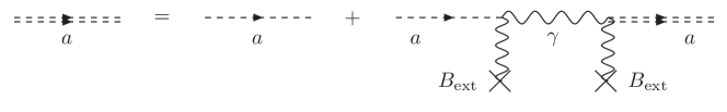
Figure 1: Diagrammatic representation of the equation $\Delta(k)=\Delta_{F}(k)+\Delta_{F}(k)M(k)\Delta(k)$ for the exact axion propagator in the external magnetic field $\mathbf{B}_{\rm ext}$. The sources of this are denoted by crosses. The dashed lines represent the free axion propagator, while the double dashed ones represent the exact propagator. The internal waved line stands for the exact photon propagator in the external magnetic field.

Formally, the exact photon propagator $\mathcal{D}_{\mu\nu}$ is given by the Dyson relation

$$\mathcal{D}^{-1}(k)=D^{-1}(k)-\Pi(k),$$ (11)

where $D_{\mu\nu}=\langle\mu|D(k)|\nu\rangle=k^{2}g_{\mu\nu}-\zeta k_{\mu}k_{\nu}$ is the free propagator and $\zeta$ is the gauge parameter. The polarization tensor $\Pi$ is diagonalizable and its 4 eigenvectors $|e^{(i)}\rangle$, $i=1,..,4$ satisfy the orthonormality $\langle e^{(i)}|e^{(j)}\rangle=\delta_{ij}$ and completeness $\sum|e^{(i)}\rangle\langle e^{(i)}|=1$ relations Shabad . Because of the transversality condition, $k\cdot\Pi=\Pi\cdot k=0$, the polarization tensor has a zero eigenmode directed along $k$. To keep the same notation as in Ref. Shabad , we label this as the fourth eigenvector $e_{\mu}^{(4)}=\langle\mu|e^{(4)}\rangle=k_{\mu}/|k|$. So we find

$$\Pi=\sum_{i=1}^{3}\lambda_{i}|e^{(i)}\rangle\langle e^{(i)}|,$$ (12)

where we have indicated with

$$\lambda_{i}=\langle e^{(i)}|\Pi|e^{(i)}\rangle=e_{\mu}^{*(i)}\Pi_{\mu\nu}e_{\nu}^{(j)}$$ (13)

the eigenvalue associated with $|e^{(i)}\rangle$. Of course, it results $\lambda_{4}=0$. Using the orthonormality and completeness relations, it is easy to invert Eq. (11) to get a formal expression for the exact photon propagator

$$\mathcal{D}=\sum_{i=1}^{3}\frac{|e^{(i)}\rangle\langle e^{(i)}|}{k^{2}-\lambda_{i}}+(1-\zeta)\frac{|e^{(4)}\rangle\langle e^{(4)}|}{k^{2}}\>.$$ (14)

In an external magnetic field the relevant term of the axion-photon interaction (2) can be conveniently written as

$$\mathcal{L}_{a\gamma}=g_{a\gamma}a\,\widetilde{F}_{\rm ext}^{\mu\nu}\,\partial_{\mu}A_{\nu}.$$ (15)

Observing that the vector $e^{(3)}_{\mu}=k^{\nu}\widetilde{F}^{\rm ext}_{\nu\mu}/(|k_{\parallel}|B)$ directed along $\mathbf{B}_{\rm ext}$ is an eigenvector because of the azimuthal symmetry induced by $\mathbf{B}_{\rm ext}$, this interaction takes (in momentum space) the particularly simple form

$$\mathcal{L}_{a\gamma}=-ig_{a\gamma}\,|k_{\parallel}|B\,aA^{\mu}e_{\mu}^{(3)}.$$ (16)

Using the orthogonality between the eigenvectors together with Eq. (14), we find

$$M(k)=-\frac{g_{a\gamma}^{2}B^{2}k_{\parallel}^{2}}{k^{2}-\lambda_{3}}\,,$$ (17)

where the eigenvalue $\lambda_{3}$ is given by Eq. (13). In the limit $\mathbf{k}\rightarrow 0$, it results $\lambda_{3}=\Pi_{33}$. Let us define the function $\mathcal{P}(k_{0})$ such that

$$\frac{\alpha_{\rm em}}{3\pi}\,\mathcal{P}(k_{0})\equiv-\frac{\Pi_{33}(k_{0},\mathbf{k}\rightarrow 0)}{k_{0}^{2}}\,,$$ (18)

where we have introduced the factor $\alpha_{\rm em}/3\pi$ for convenience. It results

$$M(k_{0})=-\frac{g_{a\gamma}^{2}B^{2}}{1+(\alpha_{\rm em}/3\pi)\mathcal{P}(k_{0})}\,.$$ (19)

The one loop polarization tensor at finite temperature in an arbitrary magnetic field was computed using the imaginary time formalism in Ref. Alexandre . In the imaginary time formalism, the (Euclidean) photon energy is quantized and expressed in terms of the so-called Matsubara frequencies: $k_{4}=-ik_{0}\rightarrow\omega_{n}=2\pi nT$, with $n$ integer. For simplicity, we consider only the contribution of the electrons in the fermion loop since this is the leading one as electrons are the lightest charged fermions. In any case, the contribution from the other fermions can be easily included. The electron energy in the fermion loop is quantized as well, $p_{4}=-ip_{0}\rightarrow\omega_{l}=(2l+1)\pi T$, with $l$ integer. The function $\mathcal{P}(\omega_{n})$ is given in Ref. Alexandre . However, for our purpose, the computation of the effective axion mass can be simplified observing that in all the phenomenologically relevant cases the axion mass is always smaller than the fermion masses $m_{B}\ll m_{e}$. This assumption will be verified a posteriori. Therefore, we can safely consider the limiting value $\mathcal{P}\equiv\mathcal{P}(\omega_{n}/m_{e}\rightarrow 0)$ in place of $\mathcal{P}(\omega_{n})$. So finally for the magnetic-induced axion mass we find

$$m_{B}^{2}\simeq\frac{g_{a\gamma}^{2}B^{2}}{1+(\alpha_{\rm em}/3\pi)\mathcal{P}}\,.$$ (20)

From Ref. Alexandre we have

$$\mathcal{P}=\int_{0}^{\infty}\frac{du}{u}\>e^{-um_{e}^{2}}\,\left\{3\sqrt{\pi}\sqrt{u}\,T\!\!\sum_{l=-\infty}^{\infty}\!\left[e^{-u\omega_{l}^{2}}\!\left(\!1-\frac{2}{3}\,\omega_{l}^{2}u\!\right)\!\right]\!\overline{u}\coth\overline{u}-1\!\right\},$$ (21)

where $\overline{u}=eBu$. Observe that the above expression is convergent and the last term in the right hand side of Eq. (21) represents the contact term which removes the ultraviolet divergence ($u\rightarrow 0$). The normalization chosen gives $m_{B}=0$ in the zero temperature and zero magnetic field limit.

III.1 IIIa. Low Temperature Limit

Before a complete analysis of expression (21) let us consider its low temperature limit $\mathcal{P}_{0}$. Actually, the computation of $\mathcal{P}_{0}$ is straightforward since in the limit $T\rightarrow 0$ the sum over the Matsubara frequencies of the electrons can be substituted by an integral over the (Euclidean) electron energy: $T\sum_{l}\rightarrow(2\pi)^{-1}\!\int dp_{4}$. The result,

$$\mathcal{P}_{0}=\lim_{T\rightarrow 0}\mathcal{P}=\int_{0}^{\infty}\frac{du}{u}\,e^{-um_{e}^{2}}\left[\overline{u}\coth\overline{u}-1\right],$$ (22)

is in agreement with the existent literature (see Ref. Mikheev ). To have a better comparison with the non-zero temperature result it is convenient to introduce the dimensionless variable

$$\lambda=\frac{B}{B_{c}}=\frac{eB}{m_{e}^{2}}\,,$$ (23)

so that

$$\mathcal{P}_{0}=\int_{0}^{\infty}\!dse^{-s/\lambda}\left[\coth{s}-\frac{1}{s}\right].$$ (24)

(The parameter $B_{c}=m_{e}^{2}/e\simeq 4.4\times 10^{13}\mbox{G}$ is known as the critical or the “Schwinger value” for the magnetic field.) A good approximation of the above integral (see Fig. 2) is given by the following expression:

Figure 2: The continuous line represents the function $P_{0}$ in Eq. (24), while the dotted line is its approximate profile Eq. (25).

$$\mathcal{P}_{0}\simeq\lambda\coth{\lambda}-1.$$ (25)

In particular, the limit $\lambda\ll 1$ ($B\ll B_{c}$) gives $\mathcal{P}_{0}\simeq\lambda^{2}/2$, whereas in the opposite limit $\lambda\gg 1$ ($B\gg B_{c}$) we find $\mathcal{P}_{0}\simeq\lambda$. Taking into account Eq. (20), this last limit gives

$$m_{B}^{2}\simeq\frac{g_{a\gamma}^{2}B^{2}}{1+(\alpha_{\rm em}/3\pi)(B/B_{c})}\,,$$ (26)

which for $B/B_{c}\gg 3\pi/\alpha_{\rm em}\sim 10^{3}$ gives in turn the result

$$m_{B}\,\simeq\>\frac{3\pi}{\alpha_{\rm em}}\>g_{a\gamma}^{2}B_{c}B\>\simeq\>5.8\,\xi\left(\frac{B}{10^{23}\mbox{G}}\right)^{\!1/2}\frac{10^{6}\mbox{GeV}}{f_{a}}\>\mbox{eV}$$ (27)

presented in Ref. Mikheev and used in Ref. noi3 .

III.2 IIIb. Finite Temperature Results

In order to include the thermal effects it is necessary to calculate the sum over the Matsubara frequencies in Eq. (21):

$$\sum_{l=-\infty}^{\infty}\!\!e^{-u\omega_{l}^{2}}\!\left(\!1-\frac{2}{3}\;\omega_{l}^{2}u\!\right)\!.$$ (28)

This sum can be conveniently expressed in terms of the the Jacobi theta function of second kind Abramowitz ,

$$\vartheta_{2}(w,q)=2q^{1/4}\sum_{n=0}^{\infty}q^{n(n+1)}\cos[(2n+1)w].$$ (29)

Indeed, observing that

$$\sum_{l=-\infty}^{\infty}e^{-u\omega_{l}^{2}}=\vartheta_{2}(0,e^{-4\pi^{2}uT^{2}}),$$ (30)

$$\sum_{l=-\infty}^{\infty}\omega_{l}^{2}e^{-u\omega_{l}^{2}}=-\frac{d}{du}\,\sum_{l=-\infty}^{\infty}e^{-u\omega_{l}^{2}},$$ (31)

we have

$$\sum_{l=-\infty}^{\infty}\!\!e^{-u\omega_{l}^{2}}\!\left(\!1-\frac{2}{3}\;\omega_{l}^{2}u\!\right)=\left(1+\frac{2}{3}\,u\,\frac{d}{du}\right)\!\vartheta_{2}(0,e^{-4\pi^{2}uT^{2}}).$$ (32)

To proceed further, we define the function

$$\mathcal{F}(x)=\sqrt{\frac{x}{\pi}}\left(3+2x\frac{d}{dx}\right)\!\vartheta_{2}(0,e^{-4x}),$$ (33)

whose graph is shown in Fig. 3.

Figure 3: The function $\mathcal{F}(x)$ defined in Eq. (33).

Taking into account Eqs. (32) and (33), we re-cast Eq. (21) in the following form:

$$\mathcal{P}=\int_{0}^{\infty}\!ds\,e^{-s/\lambda}\left[\mathcal{F}(st^{2})\coth{s}-\frac{1}{s}\right],$$ (34)

where we have defined

$$t=\frac{\pi T}{\sqrt{eB}}\,.$$ (35)

Equation (34) is very similar to Eq. (24), except for the presence of the function $\mathcal{F}(st^{2})$. It is important to notice that the temperature enters only through $\mathcal{F}(st^{2})$, and only as $st^{2}$. Let us comment this result. First of all we see from Fig. 3 that $\mathcal{F}(x)\sim 1$ for $x$ sufficiently smaller than $1$. In addition, in Eq. (34) the parameter $\lambda$ has the role of a cutoff. Therefore, in the relevant integration region, $0<s<few\times\lambda$, it results $st^{2}<few\times\lambda t^{2}=(\pi T/m_{e})^{2}$. Then, if $T\ll m_{e}$, we can set $\mathcal{F}\sim 1$ and consequently we find the result (24). On the other hand, for $T\gg m_{e}$ and $B<T^{2}$, we find the asymptotic expansion of $\mathcal{P}$:

$$\mathcal{P}\simeq\gamma+\ln c-\ln\!\left(\frac{\pi T}{m_{e}}\right)^{\!2}\!,$$ (36)

where $\gamma\simeq 0.577$ is the Euler’s constant, $c\simeq 2/3$ is a numerical constant. If $B>T^{2}$, the above equation is still valid with $c$ a slowly decreasing function of $B/T^{2}$ (see Fig. 4).
Our numerical results are shown in Fig. 5 which represents $\mathcal{P}$ given in Eq. (34) as a function of the normalized temperature $T/m_{e}$, for different values of the parameter $\lambda=B/B_{c}$. Also represented is the asymptotic expansion Eq. (36). A look at Fig. 5 shows that for a large range of values for the external magnetic field and temperatures, the term $(\alpha_{\rm em}/3\pi)\mathcal{P}$ is much smaller than 1. In particular, this is the case for high temperatures ($T\gg m_{e}$) whatever the intensity of the magnetic field is, or for low temperatures ($T\ll m_{e}$) and magnetic fields below the critical value ($B<B_{c}$). In these cases, from Eq. (20) we get that the axion mass is well approximated by

$$m_{B}\simeq g_{a\gamma}B.$$ (37)

In order to quantify the thermal effects on the axion mass, we compare the above result with the axion mass as calculated in the zero-temperature limit and for large magnetic field (see Section IIIa). From Eqs. (27) and (37) we get

$$\frac{m_{B}^{2}(T,B)}{m_{B}^{2}(0,B)}\simeq\frac{\alpha_{\rm em}}{3\pi}\,\frac{B}{B_{c}}\,.$$ (38)

Figure 4: The function $\mathcal{P}$ defined in Eq. (34) versus the temperature for different values of the “normalized” magnetic field $b=B/T^{2}$. Dotted line: $b=100$; Dashed line: $b=50$; Long-dashed line: $b=10$; Solid line: $b=1$. For $b\lesssim 5$, all curves collapse into the line $b=1$, which is well approximated by Eq. (36).

Figure 5: Numerical representation of the function $\mathcal{P}$ given in Eq. (34) as a function of the normalized temperature $T/m_{e}$ for different values of the parameter $\lambda=B/B_{c}$. Left panel. From the top to the bottom: $\lambda=20,15,10,1$. Right panel. From the top to the bottom: $\lambda=0.8,0.6,0.4,0.2$. The tick solid line in both panels represents the asymptotic expansion (36).

Therefore, for $T\gg m_{e}$ and $B\gg B_{c}$, we find that the axion mass is strongly influenced by temperature effects. In particular, thermal effects give rise to in increment of the axion mass with respect to the zero temperature limit.

Before closing this section, a comment is in order. The complete result in Eq. (36) is somewhat puzzling, since it gives a singular limit when $m_{e}\rightarrow 0$, whereas we would expect $m_{B}\rightarrow 0$ in the chiral limit, as discussed in Section II. However, it is easy to understand that this limit can not be considered in our discussion. In fact, the approach that we have considered is based on the perturbative expansion of Fig. 1, and loses clearly its validity if $M(k)$ is arbitrarily large, as in the case of very small electron mass. Indeed, our result is based on an even stronger assumption, which is that the electron mass is always much larger than the axion mass. Therefore, the result (20) is valid only if the inequality

$$\left(\frac{g_{a\gamma}B}{m_{e}}\right)^{\!2}\,\frac{1}{1+(\alpha_{\rm em}/3\pi)\mathcal{P}}\ll 1$$ (39)

is verified, which is not the case in the chiral limit. However, for the standard value of the electron mass, the above inequality is essentially always verified in any physical interesting case. In fact, even in the “worst” case $\mathcal{P}\ll 1$ (which refers to the case $T\ll m_{e}$ and $B\ll B_{c}$, or to the case $T\gg m_{e}$), the above condition translates in

$$B\ll 10^{28}\,\frac{f_{a}}{10^{9}\mbox{GeV}}\>\mbox{G},$$ (40)

which is satisfied, even in the most conservative case $f_{a}=10^{9}\mbox{GeV}$, by any cosmological and astrophysical magnetic field present in the universe below the electroweak phase transition Magnetic .

IV IV. Conclusions

The phenomenology of the axion in an external magnetic field has been deeply studied in the last few decades. Nowadays the relevance of an in depth understanding of the effects of axion interaction in an external magnetic field to astrophysics and cosmology is clear. In this paper we have further investigated this problem computing the axion mass induced by an external magnetic field. The origin of this phenomenon is related to the generation of magnetic helicity, induced by the axion itself. We computed the resulting induced mass in one loop approximation, accounting for the thermal corrections, and with no restriction on the intensity of the magnetic field. Our result is given in Eqs. (20) and (34) (see also Figs. 4 and 5), and indicates that thermal effects are not relevant for temperatures significantly below the electron mass. For $T\ll m_{e}$ our result is indeed in agreement with the existent literature. However, for higher temperatures, the axion mass is strongly influenced by temperature effects if the external magnetic field is much stronger than the Schwinger value, $B\gg B_{c}\sim 10^{13}\mbox{G}$. In this case, thermal effects give rise to an increment of the axion mass with respect to the zero temperature limit, which is proportional to the magnetic field: $m_{B}^{2}(T,B)/m_{B}^{2}(0,B)\simeq(\alpha_{\rm em}/3\pi)\,(B/B_{c})$.

It is clear that the value of the magnetic field that could induce a sizable change of the axion dispersion relation is very high, and certainly well above the possibility of the present terrestrial experiments. However, in an astrophysical or cosmological contest the magnetic induced mass could play an important role. This topic will be the object of future investigations.

- (1) R. D. Peccei and H. R. Quinn, Phys. Rev. D 16, 1791 (1977); S. Weinberg, Phys. Rev. Lett. 40, 223 (1978); F. Wilczek, ibid. 40, 279 (1978).
- (2) J. E. Kim, Phys. Rept. 150 (1987) 1; H. Y. Cheng, ibid. 158 (1988) 1.
- (3) G. G. Raffelt, Phys. Rept. 198 (1990) 1; M. S. Turner, ibid. 197 (1990) 67.
- (4) J. E. Kim, Phys. Rev. Lett. 43 (1979) 103; M. A. Shifman, A. I. Vainshtein, and V. I. Zakharov, Nucl. Phys. B 166 (1980) 493.
- (5) Recently, it was pointed out in S. Hannestad, A. Mirizzi, and G. Raffelt, JCAP 0507, 002 (2005), that the study of cosmological large-scale structures suggests that the hadronic axion window could be closed.
- (6) Z. Berezhiani, L. Gianfagna, and M. Giannotti, Phys. Lett. B 500 (2001) 286; L. Gianfagna, M. Giannotti, and F. Nesti, JHEP 0410 (2004) 044; G. R. Dvali, hep-ph/9505253; M. Giannotti, Int. J. Mod. Phys. A 20, 2454 (2005); G. Lazarides, C. Panagiotakopoulos, and Q. Shafi, Phys. Lett. B 192, 323 (1987); G. Lazarides, R. K. Schaefer, D. Seckel, and Q. Shafi, Nucl. Phys. B 346, 193 (1990). See also references in G. Lazarides, hep-ph/0601016.
- (7) R. Davis, Phys. Lett. B 180, 225 (1986); M. Y. Khlopov, A. S. Sakharov, and D. D. Sokoloff, Nucl. Phys. Proc. Suppl. 72, 105 (1999), and references therein.
- (8) G. Raffelt and L. Stodolsky, Phys. Rev. D 37, 1237 (1988).
- (9) P. Sikivie, Phys. Rev. Lett. 51, 1415 (1983); Phys. Rev. D 32, 2988 (1985); hep-ph/0606014; L. Duffy et al., Phys. Rev. Lett. 95, 091304 (2005); D. Kang, hep-ex/0605049; K. Zioutas et al. [CAST Collaboration], Phys. Rev. Lett. 94, 121301 (2005); E. Zavattini et al. [PVLAS Collaboration], Phys. Rev. Lett. 96, 110406 (2006).
- (10) L. A. Vasilevskaya, N. V. Mikheev, and A. Y. Parkhomenko, Phys. Atom. Nucl. 64, 294 (2001) [Yad. Fiz. 64, 342 (2001)]; N. V. Mikheev, A. Y. Parkhomenko, and L. A. Vasilevskaya, Prepared for International Workshop on Strong Magnetic Fields in Neutrino Astrophysics, Yaroslavl, Russia, 5-8 Oct 1999.
- (11) L. Campanelli and M. Giannotti, Phys. Rev. Lett. 96, 161302 (2006).
- (12) A. A. Anselm and N. G. Uraltsev, Phys. Lett. B 114, 39 (1982); A. A. Anselm and A. R. Nunes, Sov. J. Nucl. Phys. 48, 1079 (1988) [Yad. Fiz. 48, 1793 (1988)].
- (13) C. Csaki, N. Kaloper, and J. Terning, Phys. Rev. Lett. 88, 161302 (2002); C. Csaki, N. Kaloper, M. Peloso, and J. Terning, JCAP 0305, 005 (2003).
- (14) A. Mirizzi, G. G. Raffelt, and P. D. Serpico, Phys. Rev. D 72, 023501 (2005); A. Mirizzi, G. G. Raffelt, and P. D. Serpico, astro-ph/0607415.
- (15) D. J. Gross, R. D. Pisarski, and L. G. Yaffe, Rev. Mod. Phys. 53, 43 (1981).
- (16) L. Campanelli and M. Giannotti, Phys. Rev. D 72, 123001 (2005).
- (17) R. Jackiw and S. Y. Pi, Phys. Rev. D 61, 105015 (2000).
- (18) G. B. Field and S. M. Carroll, Phys. Rev. D 62, 103008 (2000).
- (19) A. E. Shabad, Annals Phys. 90, 166 (1975).
- (20) J. Alexandre, Phys. Rev. D 63, 073010 (2001).
- (21) L. Campanelli and M. Giannotti, astro-ph/0512324, to appear in JCAP.
- (22) M. Abramowitz and I. A. Stegun, Handbook of Mathematical Functions with Formulas, Graphs, and Mathematical Tables (Dover, New York, 1964).
- (23) For reviews on cosmic magnetic fields see: M. Giovannini, Int. J. Mod. Phys. D 13, 391 (2004); hep-ph/0208152; hep-ph/0111220; L. M. Widrow, Rev. Mod. Phys. 74, 775 (2003); D. Grasso and H. R. Rubinstein, Phys. Rept. 348, 163 (2001); J. P. Vallée, New Astr. Rev. 48, 763 (2004); A. D. Dolgov, hep-ph/0110293; V. B. Semikoz and D. D. Sokoloff, Int. J. Mod. Phys. D 14, 1839 (2005); P. P. Kronberg, Rept. Prog. Phys. 57, 325 (1994).