Cross-fertilization of QCD and statistical physics:
high energy scattering, reaction-diffusion, selective evolution, spin glasses
and their connections

Abstract

High energy scattering was recently shown to be similar to a reaction-diffusion process. The latter defines a wide universality class that also contains e.g. some specific population evolution models. The common point of all these models is that their respective dynamics are described by noisy traveling wave equations. This observation has led to a new understanding of QCD in the regime of high energies, and known universal results on reaction-diffusion models could be transposed to obtain quantitative properties of QCD amplitudes. Conversely, new general results for that kind of statistical models have also been derived. Furthermore, an intriguing relationship between noisy traveling wave equations and the theory of spin glasses was found.

I Introduction

The behavior of hadronic cross sections at high energy has been the subject of intense theoretical and experimental investigations for several decades. These studies will become even more relevant with the advent of the LHC, where protons will collide at a center-of-mass energy of 14 TeV.

In the following, we will focus on the forward elastic amplitude $A(Y,k)$ for the scattering of two hadronic objects at total rapidity $Y$, one of the objects (called the probe) being characterized by a tunable momentum $k$, that defines the scales in the plane transverse to the collision axis. The other hadron will be called the target. The scattering occurs at a given impact parameter that, here, will be fixed. Experimentally, the corresponding process could be, for example, deep-inelastic electron-proton (or nucleus) scattering, in which case $k$ would be of order of the virtuality of the exchanged photon. The total rapidity $Y$ can be seen as the rapidity of the target in the rest frame of the probe: It is related to the squared center-of-mass energy $s$ through $Y=\ln(s/k^{2})$. Note that one could equally well work in transverse coordinates instead of momenta, which proves useful in many cases: In coordinate space, $\tilde{A}(Y,r)$ is directly related to the probability that the probe of size $r$ interact with the evolved target at the considered impact parameter, which in particular results in the unitarity bound $\tilde{A}\leq 1$. The relationship between the two representations of the amplitude reads

$$\tilde{A}(Y,r)=r^{2}\int\frac{d^{2}k}{2\pi}e^{ik\cdot r}A(Y,k).$$ (1)

Although total cross sections are not computable from standard QCD methods since confinement effects necessarily enter, the evolution with rapidity of the scattering amplitudes for a localized probe at a given impact parameter (understood in Eq. (1)) may be obtained starting from perturbative calculations that lead e.g. to the Balitsky hierarchy of equations B . In the latter framework, the evolution of $\tilde{A}$ reads

$$\partial_{\bar{\alpha}Y}\tilde{A}(Y,r)=\int\frac{d^{2}z}{2\pi}\frac{r^{2}}{z^{2}(r-z)^{2}}(\tilde{A}(Y,z)+\tilde{A}(Y,r-z)\\ -\tilde{A}(Y,r)-\langle\tilde{T}(Y,z)\tilde{T}(Y,r-z)\rangle),$$ (2)

where $\bar{\alpha}=\frac{\alpha_{s}N_{c}}{\pi}$. One had to introduce $\tilde{T}$ which is meant to be the scattering amplitude off one particular configuration of the target. It is its average over all quantum fluctuations of the latter that corresponds to the physically measurable amplitude: $\tilde{A}=\langle\tilde{T}\rangle$.

Eq. (2) is not closed: One needs a further evolution equation for $\langle\tilde{T}\tilde{T}\rangle$. Eq. (2) is only the first equation of an infinite hierarchy which involves increasingly complex mathematical objects. Solving that system is a formidable task, and not surprisingly, no one has found a solution from a direct study of Eq. (2). Another problem with the hierarchy is that it is not clear whether its complete form for arbitrary targets is known.

A significantly simpler equation may be obtained by arbitrarily factorizing the correlator $\langle\tilde{T}\tilde{T}\rangle$ into the product $\tilde{A}\tilde{A}$, within a kind of mean field approximation that neglects fluctuations in the target. This was first proposed by Balitsky B and subsequently re-derived by Kovchegov K in the particular physical context of deep-inelastic scattering off an infinitely large nucleus. An elegant representation of the resulting equation is obtained in momentum space by using Eq. (1), namely

$$\partial_{\bar{\alpha}Y}A=\chi(-\partial_{\ln k^{2}})A-A^{2},$$ (3)

where $\chi(-\partial_{\ln k^{2}})$ is the expression of the integral kernel that appears in Eq. (2) in momentum space. The main properties of the solutions to Eq. (3) are now known LT ; MT2002 ; MP2003 ; MP2004 , but the effects of the fluctuations neglected in going to the Balitsky-Kovchegov (BK) equation (3) and even their very nature had not been appreciated until quite recently.

One may guess that one difficulty with Eqs. (2) and (3) is that they both contain nonlinearities. The latter are meant to encode parton saturation effects GLRMQ . One could think of neglecting them (by dropping the $-A^{2}$ term in Eq. (3) for example), and indeed, that used to be the usual approximation until a few years ago. The resulting equation is named after Balitsky, Fadin, Kuraev and Lipatov (BFKL) BFKL ($\chi(-\partial_{\ln k^{2}})$ that appears in Eq. (3) is called the BFKL kernel). But in 1999, Golec-Biernat and Wüsthoff showed GBW that the nonlinearities in Eqs. (2),(3) may already play an important role in the most recent data for deep-inelastic scattering (see also Ref. MSM ). Their work stirred a great theoretical interest for the full nonlinear equations. For a long time, it was the BK equation that was the focus of most of the theoretical and phenomenological works in high energy QCD, despite the relative arbitrariness of the approximations made to get it. Only in 2004 did Mueller and Shoshi address the problem of trying to quantify effects beyond those described by the BK equation, using a very original approach MS2004 . Subsequently, a deep interpretation of what they had done in relation with problems of statistical mechanics was found M2005 ; MP2004 ; EGBM2005 , which paved the way for a new and fruitful understanding of high energy QCD.

The goal of these two lectures is to show that high energy scattering looks very much like some processes (called reaction-diffusion) that appear in other physical, biological, or chemical contexts. We will provide a very simple and transparent picture of high energy QCD, but accurate enough to enable one to get presumably exact analytical results for QCD. The first lecture (Sec. II) aims at establishing this correspondence. “Cross-fertilization” is the title of these lectures because while investigating this relationship, we were able to also derive some general results that apply to a wider context. The second lecture (Sec. III) reviews them. The most important of these results may directly be transposed to QCD. Throughout, the focus will be put on the underlying physical ideas rather than on the technicalities (references to original work where details are worked out will be provided whenever necessary). We would like the reader to appreciate that this business was made possible by coming back to the basic concepts of high energy scattering in the parton model in the light of apparently completely unrelated physics, rather than trying to address directly the very technical equations that have been established for QCD.

II High energy QCD as a statistical process

II.1 What is universality?

Our first task is to understand that it may sometimes be fruitful to replace a complicated problem (like QCD evolution, see Eq. (2)) by a much simpler one (reaction-diffusion in our case, as we will see in these lectures), and yet be able to get quantitative results from the solution to the latter. This is possible when both models, the simple and the complicated ones, belong to the same universality class.

The concept of universality was introduced in the 60’s by a bunch of renowned physicists, among whom Widom, Kadanoff, Fisher and Wilson in the theory of critical phenomena. To illustrate it, let us consider a system of spins, that is a set of binary variables $S_{i}=\pm 1$, on a two-dimensional lattice and interacting through the Hamiltonian

$$H=-\sum_{i,j}J_{ij}S_{i}S_{j}.$$ (4)

If $J_{ij}=J>0$ when the sites $i$ and $j$ are nearest neighbors and 0 otherwise, this is the Ising model with ferromagnetic interactions. The partition function is given by

$$Z=\sum_{\{S_{i}\}}e^{-H[\{S_{i}\}]/k_{B}T}$$ (5)

at a given temperature $T$.

At high temperature, all spin configurations have equal probability. At low temperature, only a few configurations have a significant probability, the ones that minimize the energy. The minimum energy configuration is the one in which all spins are aligned. Near the critical point, the average magnetization reads

$$\langle S_{i}\rangle\sim(T_{c}-T)^{\beta},$$ (6)

and an exact calculation gives $\beta=1/8$ for two-dimensional systems, as may be checked in standard statistical mechanics textbooks.

The Ising model may represent only a very idealized magnet. One may wonder why it is interesting to study extensively such an over-simplified model, which obviously incorporates only a few very basic properties of magnetic materials and neglects many others. Well, it turns out that the exponent $\beta$ (as well as a few other exponents) is completely independent of the microscopic details of the system, which means that it is the exact result also for realistic magnets. Of course, other quantities strongly depend on those details: This is the case for the critical temperature $T_{c}$ for example.

The universality class is defined only by very general properties of the system, like the space dimension, and the symmetries. All systems that share these few properties are expected to bear the same critical exponents. So if one is able to solve the simplest model, one is likely to know important features of all representatives of its universality class.

High energy QCD has little to do with the Ising model and with criticality. We are now going to introduce a class of systems which, as we will argue later on, are likely to share universal properties with high energy QCD.

II.2 Warm-up: Properties of a stochastic zero-dimensional model

We address the time evolution of a system of $n(t)$ particles that obey the following rules: In each time interval $dt$, each single particle has a probability $dt$ to split in 2 particles, and a probability $(n(t)-1)dt/N$ to disappear. This yields:

$$n(t+dt)=\left\{\begin{aligned} n(t)\!+\!1&\text{ proba }dt\\ n(t)\!-\!1&\text{ proba }\frac{(n(t)\!-\!1)dt}{N}\\ n(t)&\text{ proba }1\!-\!dt-\frac{(n(t)\!-\!1)dt}{N}.\end{aligned}\right.$$ (7)

One may represent the evolution of the system in the form of a stochastic evolution equation:

$$\frac{dn}{dt}=n-\frac{n(n-1)}{N}+\sqrt{n+\frac{n(n-1)}{N}}\,\nu,$$ (8)

where $\nu$ is a noise (i.e. a random function of time) of zero average and of variance satisfying $\langle\nu(t)\nu(t^{\prime})\rangle=\delta(t-t^{\prime})$. This means that $\nu$ typically varies by 1 unit when $t$ is changed by 1. It is a simple exercise to derive Eq. (8): It is enough to compute the mean $\langle n(t+dt)\rangle$ and variance $\langle n^{2}(t+dt)\rangle$ given $n(t)$ from the stochastic rules (7).

We see on Eq. (8) that in a typical realization, the number of particles will start to grow exponentially (linear term) until $n(t)\sim N$, at which point a steady state is reached (nonlinear term), up to random fluctuations (noise term).

Solving the model consists in exhibiting the statistics of $n(t)$. In a first approach, one may simulate numerically different realizations of the model, and then perform the average over the realizations to get $\langle n(t)\rangle$ and maybe higher-order moments of $n(t)$. This is shown in Fig. 1. One could also try to obtain an evolution equation for $\langle n(t)\rangle$ from Eq. (8) and solve it analytically. But the latter involves the correlator $\langle n^{2}\rangle$:

$$\frac{d\langle n\rangle}{dt}=\langle n\rangle-\frac{\langle n(n-1)\rangle}{N},$$ (9)

and thus one eventually needs to solve an infinite hierarchy of coupled equations. This set of equations is qualitatively similar to the Balitsky hierarchy (2). Only through a mean field approximation, consisting in factorizing all correlators and valid in the large-$N$ limit does Eq. (9) boil down to a closed equation

$$\frac{d\langle n\rangle}{dt}=\langle n\rangle-\frac{\langle n\rangle^{2}}{N}.$$ (10)

This is the equivalent of the BK equation (3). Unfortunately, the solution to this much simpler equation is quite far from the complete solution to Eq. (8) or (9) (see Fig. 1), and it is manifest that more sophisticated approaches to the full stochastic model are needed.

To address the complete stochastic model (7), we can think of two possible ways. One may compute iteratively the successive orders in $1/N$ by field-theoretical methods and perform a resummation: This method was pushed quite far in Ref. SX2005 . Another possible path is to notice that the noise is actually important only as long as the number of particles $n(t)$ is small: For large $n(t)$, the evolution is essentially deterministic. For small $n(t)$ instead, it is the nonlinearity in Eq. (8) that is negligible, which makes the evolution tractable, even analytically in this simple zero-dimensional case. That was investigated in Ref. M2006 .

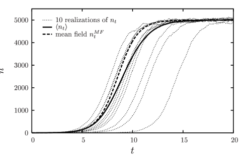
Figure 1: (From Ref. M2006 ). Ten realizations of the evolution (7) of the zero-dimensional toy model (dotted lines), together with the full solution for $\langle n(t)\rangle$ (full line) and the solution of the mean-field equation (10) (dashed line). $N$ is set to 5000 in this example.

II.3 Universality class of traveling wave equations

We now add a spatial dimension to the model. We consider $n(t,x)$ particles at time $t$ and on each site $x$ of a one-dimensional lattice. In addition to the rules (7) that apply on each site, a given particle at $x$ has some probability $p$ to jump to the nearby sites $x+\Delta x$ or $x-\Delta x$. The evolution of one realization may then be written as

$$\frac{dn(t,x)}{dt}=p[n(t,x+\Delta x)+n(t,x-\Delta x)-2n(t,x)]\\ +n(t,x)-\frac{n(t,x)(n(t,x)-1)}{N}+\sqrt{n(t,x)}\,\nu,$$ (11)

where $\nu$ is again a noise of zero mean that varies by typically 1 when $x$ or $t$ are changed by one unit. This equation is very close to Eq. (8) except for a new diffusion term (inside the square brackets) that correlates nearby spatial sites.

Both in Eq. (8) and in Eq. (11) the noise term is of order $\sqrt{n}$. This is typical of a statistical noise associated to discrete systems of particles: Indeed, adding stochastically $n$ particles on the average to a system means adding a number of particles typically in the range $n\pm\sqrt{n}$ in a given realization. Hence the noise term is directly related to discreteness.

Let us follow a particular realization of the evolution of the system. Starting from a given initial condition (for example a bunch of particles localized around some given lattice site), the number of particles grows exponentially on each occupied site until it reaches $N$, at which point the growth stops because the positive growth term $n$ is exactly compensated by the negative nonlinear term $-n^{2}/N$. At this point, only fluctuations of order $\sqrt{N}$ are left in the evolution. At the same time, diffusion takes place, allowing the particles to “escape” toward larger (or lower) values of $x$ (there is a symmetric front traveling to the left if the initial condition is local). It is then clear that the solution will look like a noisy wave front, that connects a region (say to the right) where there is no particle to a region (to the left) where the equilibrium number of particles per site $N$ is reached. This wave front “travels” toward larger values of $x$, and is therefore called a traveling wave. One step of the evolution is illustrated in Fig. 2.

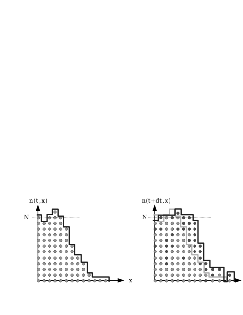
(a)                                       (b)

Figure 2: Sketch of one step of the evolution of a realization in the one-dimensional model (from (a) to (b); $N=12$ here). The dark disks represent the particles that have been added or that have diffused. For the smallest values of $x$, some particles have also disappeared, so that the maximum particle number does not exceed $N$ on the average, up to fluctuations of order $\sqrt{N}$ authorized by the stochastic term in Eq. (11).

The model that we have outlined is a typical reaction-diffusion process. The name “reaction-diffusion” stems from chemistry: Such a process may be a (very crude) model for chemical reactions. Renormalizing the number of particles through the introduction of $u=n/N$, one may write the general structure of the evolution of such a system in the following form:

$$\partial_{t}u=\underset{\text{branching diffusion}}{\underbrace{\chi(-\partial_{x})u}}-\underset{\text{compensates the growth of $u$ near 1}}{\underbrace{\text{nonlinear function of $u$}}}\\ +\underset{\text{encodes discreteness}}{\underbrace{\text{noise of order}\sqrt{\frac{u}{N}}}}.$$ (12)

$\chi(-\partial_{x})$ is a kernel that encodes branching diffusion. It could be a differential operator such as $\partial_{x}^{2}+1$ (which would correspond to carefully performing the limit $\Delta x\rightarrow 0$ in the above example) or, more generally, an integral operator (which is the case in QCD).

The universality class defined by Eq. (12) is usually named after Fisher and Kolmogorov-Petrovsky-Piscounov (F-KPP) FKPP1937 , who for the first time formulated mathematically such processes. For a given stochastic equation, there is no general theorem to decide whether it belongs to the same class as Eq. (12) or not. It is rather a matter of guess from the physical properties of the underlying model. One knowns however that the exact form of the nonlinearity in Eq. (12) is not important. It could be any reasonable power of $u$, for example. Also the precise form of the noise is not an issue and does not affect the properties of the solutions at large $N$: One could have a slightly modified form, for example $\sqrt{u(1-u)/N}$. The only important feature is that it should scale like $\sqrt{u/N}$ for small values of $u$.

We are now going to give some basic properties of the solutions to F-KPP-like evolution equations P2004 . More details and a review of the latest developments will be provided in Sec. III.

The traveling wave that develops at large times is characterized by its mean shape and by the statistics of its position $X_{t}$. The latter may be defined, for example, as the value of $x$ for which $u$ has a definite value $u_{0}$, for instance $u_{0}=1/2$. It is known since the seminal papers of Brunet and Derrida BD that for large times and large $N$, $X_{t}$ has the following mean and variance:

$$\begin{split}&\langle X_{t}\rangle=\left(\frac{\chi(\gamma_{0})}{\gamma_{0}}-\frac{\pi^{2}\gamma_{0}\chi^{\prime\prime}(\gamma_{0})}{2\ln^{2}N}\right)t\\ &\langle X_{t}^{2}\rangle-\langle X_{t}\rangle^{2}\sim\frac{t}{\ln^{3}N}.\end{split}$$ (13)

The average is taken over many realizations of the evolution (12), and $\chi(\gamma)$ is the characteristic function of the diffusion kernel (i.e. the eigenvalue of $\chi(-\partial_{x})$ that corresponds to the eigenfunction $e^{-\gamma x}$). $\gamma_{0}$ solves $\chi(\gamma_{0})=\gamma_{0}\chi^{\prime}(\gamma_{0})$. The shape of each realization is, up to some noise

$$u(t,x)=e^{-\gamma_{0}(x-X_{t})}.$$ (14)

A numerical evolution of a stochastic model of the F-KPP type is displayed in Fig. 3. One sees the universality in shape of each individual realization as well as the dispersion in front positions between different realizations, that indeed grows like $\sqrt{t}$ (see Eq. (13)). We will come back to the derivation of these results in Sec. III.

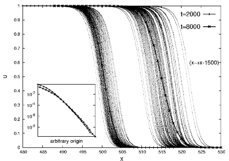
Figure 3: (From Ref. EGBM2005 ). 100 realizations of the evolution of a stochastic traveling wave model, at two different times. The averages over the realizations (that corresponds to the physical amplitude in QCD, see the dictionary (18)) are shown in full line. Inset: the average $\langle u\rangle$ over the different realizations, shifted in time and superimposed in order to show the mismatch in slopes.

II.4 Evolution of QCD amplitudes

With the intuition gained by studying simple particle models, we are now in position to argue that high energy scattering naturally belongs to the universality class of the stochastic F-KPP equation.

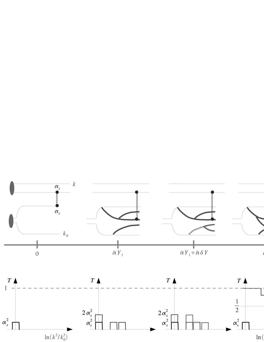
Figure 4: One realization of the evolution of an onium-onium scattering amplitude. At zero rapidity (leftmost plots), the amplitude consists in a bare gluon exchange between the probe (of size $1/k$; upper bubble) and the target (of size $1/k_{0}$; lower bubble): $T=\alpha_{s}^{2}$ if the momentum scales of the two objects match, $T=0$ otherwise. When rapidity is increased (going from the left to the right), each gluon in the Fock state of the target may split in two gluons of similar transverse momenta, and this process drives an exponential increase of the amplitude for $k$ around $k_{0}$, up to a diffusion. Eventually (rightmost plots), this growth has to slow down when $T\sim 1$ in order to comply with the unitarity constraints. Beyond this point, nonlinear saturation effects enter and a traveling wave forms in $T$.

We consider the scattering of two hadrons made of quark-antiquark pairs of respective sizes $1/k$ and $1/k_{0}$, to simplify the discussion (see Fig. 4). We assume that these hadrons are small enough (much smaller than $1/\Lambda_{\text{QCD}}$) so that perturbation theory applies.

If there is few energy available for the scattering (the hadrons interact almost at rest), then typically they are in their valence configuration. Their interaction consists in exchanging one gluon when they are of similar size and at the same impact parameter: In this case, the forward elastic amplitude reads $T\sim\alpha_{s}^{2}$. If the hadrons are of very different sizes or if their impact parameters do not match, then they do not “see” each other and $T=0$. Now boost one of the hadrons, called the target: This corresponds to increasing the center-of-mass energy of the reaction. Due to the resulting opening of phase space, a typical configuration of the target is no longer the bare valence quarks, but the latter together with a number $n(Y,k)$ of gluons of transverse momentum $k$, whose mean depend on the rapidity. Correspondingly, the scattering amplitude off that particular configuration of the target reads

$$T(Y,k)\sim\alpha_{s}^{2}n(Y,k),$$ (15)

where $k$ is of the order of the inverse size of the hadronic probe. This relationship is not exact, but may be derived rigorously as a limit of QCD scattering amplitudes.

In a given realization of the Fock space of the target, the number of gluons typically doubles when $\bar{\alpha}Y$ is increased by one unit (each gluon has a probability to split in 2 gluons). The transverse momenta of the new gluons are close to the ones of their parents, up to some diffusion. This branching diffusion process is encoded in the BFKL evolution kernel $\chi$ defined in the Introduction. As we are following one given realization, that evolves randomly, the equation contains a stochastic term of order $\sqrt{n}$, i.e. $\alpha_{s}\sqrt{T}$ from Eq. (15). At this stage, we may write the evolution of the scattering amplitude off one particular realization as

$$\partial_{\bar{\alpha}Y}T=\chi(-\partial_{\ln k^{2}})T+\alpha_{s}\sqrt{2T}\nu$$ (16)

where $\nu$ is a noise of zero-mean whose variations are of order one when $\ln k^{2}$ and $\bar{\alpha}Y$ are varied by one unit.

Because $\tilde{T}$ is related to an interaction probability, $\tilde{T}\leq 1$ in appropriate normalizations and so the number of gluons of given momentum (related to $T$) cannot grow exponentially forever. Hence a negative term that becomes important when $T\sim 1$ has to enter Eq. (16). One may write M2004 ; M2005 ; EGBM2005

$$\partial_{\bar{\alpha}Y}T=\chi(-\partial_{\ln k^{2}})T-T^{2}+\alpha_{s}\sqrt{2T}\nu.$$ (17)

The physical amplitude $A$ is obtained from $T$ by taking the average over all possible Fock realizations of the target, $A=\langle T\rangle$. The mean-field approximation $\langle T^{2}\rangle=A^{2}$ of this equation precisely coincides with the BK equation (3).

Hence we are led to an equation in the same universality class as Eq. (12), with the following dictionary (compare Eq. (12) and Eq. (17)):

$$\begin{split}&u=T,\ t=\bar{\alpha}Y,\ x=\ln k^{2},\\ &N=\frac{1}{\alpha_{s}^{2}},\ \chi(-\partial_{x})=\text{BFKL kernel}.\end{split}$$ (18)

Let us comment on the physical implications of having a stochastic equation like (17) describing the dynamics. The BK equation (3) is known to admit traveling wave solutions MP2003 , whose position $X_{t}$ (which corresponds in QCD to the so-called saturation scale $Q_{s}(Y)$ through $X_{t}=\ln Q_{s}^{2}(Y)$) is a deterministic function of the rapidity. This property is related to a phenomenon observed in the deep-inelastic scattering data and called “geometric scaling” SGK2001 : The physical amplitude $A(Y,k)$ only depends on the combined variable $k^{2}/Q_{s}^{2}(Y)$, and not on $k$ and $Y$ separately. By contrast, each realization of an evolution given by Eq. (17) is a noisy traveling wave, which has a random position (i.e. saturation scale) whose statistics follow Eq. (13) (use the dictionary (18)). The consequence is that $A=\langle T\rangle$ has a peculiar scaling behavior, different from geometric scaling M2004 ; M2005 ; EGBM2005 :

$$A(Y,k)=A\left(\frac{\ln k^{2}-\bar{\alpha}Y\left(\frac{\chi(\gamma_{0})}{\gamma_{0}}-\frac{\pi^{2}\gamma_{0}\chi^{\prime\prime}(\gamma_{0})}{2\ln^{2}(1/\alpha_{s}^{2})}\right)}{\sqrt{\bar{\alpha}Y/\ln^{3}(1/\alpha_{s}^{2})}}\right),$$ (19)

which is easy to derive from Eqs. (13),(14).

Mueller and Shoshi were the first authors who noticed that geometric scaling was broken beyond the BK equation. However, the statistical interpretation given here was crucial to arrive at the correct scaling form (19) (see Ref. M2004 ).

Let us summarize the assumptions that have lead to Eqs. (17) and (19). The linear terms therein represent the perturbative splitting of the partons when rapidity increases, and may be obtained exactly e.g. in the framework of the color dipole model M1994 . We have not written down explicitely the distribution of the noise $\nu$ (we just gave its typical variations), but the solution (19) is robust with respect to its detailed form. The nonlinear term is supposed to encode parton saturation. So far, we cannot provide an exact expression for it because a QCD realization of saturation has not been derived. However, the solution (19) is also universal with respect to the form of the nonlinearities. The only really important condition for universality arguments to apply is that there should indeed be saturation, i.e. the gluon density should not be able to grow forever. Arguments for this feature were given a long time ago GLRMQ . So if the latter is true, because of the universality of some properties of solutions to Eq. (17), then we believe that Eq. (19) represents the exact asymptotics of QCD.

Last, we would like to draw the attention of the reader to the fact that we do not think that these results are very relevant phenomenologically yet, since the asymptotics show up only for $\ln 1/\alpha_{s}^{2}\gg 1$ (which means that $\alpha_{s}$ has to be unrealistically small). In our opinion, one may conduct sound phenomenological studies only once subleading effects have also been understood, beyond Eq. (19). However, numerical calculations may already provide some clues on the behavior of QCD amplitudes for more realistic values of the parameters, as explained in Ref. M2006 .

III New general results on traveling wave equations and their applications to QCD

In the previous section, we have argued that the evolution of QCD amplitudes at high energy is governed by a nonlinear stochastic evolution equation in the universality class of the stochastic Fisher and Kolmogorov-Petrovsky-Piscounov (F-KPP) equation. The latter literally reads

$$\partial_{t}u=\partial^{2}_{x}u+u-u^{2}+\sqrt{\frac{2}{N}u(1-u)}\nu,$$ (20)

where $\nu$ is a normal Gaussian noise, uncorrelated both in $t$ and in $x$. The deterministic part of this equation (obtained by setting $\nu=0$) was first written in 1937 in the context of studies of the spread of genes (or diseases) in a population FKPP1937 . Only in 1983 some properties of its solutions were rigorously derived P2004 . In particular, it was understood that the large-time solutions were traveling waves. The dominant effect of the noise term in Eq. (20) on the shape and velocity of the wave front was worked out by Brunet and Derrida in 1997. Note that the scaling form of the dispersion in the front position had only been measured numerically. We have recently been able to make progress on the statistics of the position of the front BDMM2005 .

In practice, we will discuss the more general equation (12), of which Eq. (20) is just a particular case.

III.1 More on the propagation of noisy traveling waves

III.1.1 Solving the deterministic F-KPP equation

First, we address the deterministic version of Eq. (20), namely

$$\partial_{t}u=\chi(-\partial_{x})u-u^{2}.$$ (21)

The choice $\chi(-\partial_{x})=\partial_{x}^{2}+1$ would correspond to Eq. (20) exactly, but we keep the branching diffusion terms in a more general form in order to be able to easily transpose the results to other contexts, such as the QCD evolution equations.

In the case of the deterministic F-KPP equation, there are two fixed points, $u=0$ and $u=1$ which are respectively unstable and stable under small perturbations. Starting from a localized initial condition, the branching diffusion encoded in $\chi$ leads to a local exponential growth of $u$ and a spread in $x$. When $u$ becomes close to 1, then the nonlinear term tames the growth so that $u$ does not get bigger than 1. This mechanism leads to a wave front that invades larger values of $x$ when time flows, being pulled by its tail.

One may compute the asymptotic velocity of the front in a very simple way. Indeed, because the wave front is “pulled” by its low density tail, where the nonlinearity is negligible, it is enough to solve the linear part of Eq. (21) to understand the properties of the wave front.

Consider a front decaying like $u_{\gamma}=e^{-\gamma(x-v(\gamma)t)}$, with $\gamma$ a given wave number and $v(\gamma)$ its velocity. Then it is clear from Eq. (21) that

$$v(\gamma)=\frac{\chi(\gamma)}{\gamma}.$$ (22)

The general solution is a linear superposition of $u_{\gamma}$,

$$u(t,x)=\int d\gamma f(\gamma)e^{-\gamma(x-v(\gamma)t)}$$ (23)

where $f(\gamma)$ is a representation of the initial condition.

Let us concentrate on the large-time behavior of the solution. We are following the wave around a fixed value of $u$ (since the nonlinearity forces $u$ to range between 0 and 1), so the large-$t$ limit has to be performed in the frame of the wave defined by the change of variable $x_{\text{WF}}=x-V_{\infty}t$, where $V_{\infty}$ is the asymptotic velocity of the wave. After replacement of $x$ in Eq. (23), the saddle point condition reads $V_{\infty}=\chi^{\prime}(\gamma)$. Matching this expression with Eq. (22), we find that the wave number $\gamma_{0}$ that dominates asymptotically solves $\chi(\gamma_{0})/\gamma_{0}=\chi^{\prime}(\gamma_{0})$, i.e. $\gamma_{0}$ minimizes $v(\gamma)$. Thus the asymptotic form of the wave front reads

$$\begin{split}u(t\rightarrow\infty,x)\sim e^{-\gamma_{0}(x-v(\gamma_{0})t)}\ \ &\text{ for }\ \ x\gg v(\gamma_{0})t,\\ &\text{ with }\ v^{\prime}(\gamma_{0})=0.\end{split}$$ (24)

(The complete discussion may be found in Ref. MP2003 ). This is the large time solution, but the front shape and velocity are also known at subasymptotic times. Let $X_{t}$ be the position of the front, defined e.g. by $u(t,X_{t})=u_{0}$, where $u_{0}$ is a constant between 0 and 1. Then if the initial condition is localized enough, the wave front has the shape M2004

$$u(t,x)\sim(x-X_{t})\exp\left(-\frac{(x-X_{t})^{2}}{2\chi^{\prime\prime}(\gamma_{0})t}\right)e^{-\gamma_{0}(x-X_{t})}$$ (25)

and the front velocity reads

$$v_{t}=\frac{dX_{t}}{dt}=\frac{\chi(\gamma_{0})}{\gamma_{0}}-\frac{3}{2\gamma_{0}t}.$$ (26)

The asymptotic velocity $V_{\infty}$ (first term) is reached quite slowly. One more term is known in this large-$t$ expansion MP2004 , but we will not discuss it here. We may comment that the velocity (26) corresponds to the velocity of a front that has reached its asymptotic shape (24) only in the range

$$(x-X_{t})^{2}<2\chi^{\prime\prime}(\gamma_{0})t.$$ (27)

This is indeed the range in which the Gaussian factor in Eq. (25) is close to a constant.

III.1.2 Hacking the deterministic equation to simulate discreteness

Now we go back to the original stochastic equations (12) or (20). Generally speaking, what we missed when we neglected the noise is mainly the discreteness of $u$. Think of a particle model on a lattice: $u$ can take the values $1/N$, $2/N$, $3/N$…but not fractions of these numbers, a feature which of course was completely neglected in Eq. (21), as can be seen on the solution (24). For $u\gg 1/N$, this might not be a problem, but for $u\sim 1/N$, neglecting discreteness may prove very wrong, especially since the propagation of the wave front is very sensitive to its tail.

Brunet and Derrida came up with the idea that this discreteness could be incorporated back into the deterministic equation (21) by simply adding a cutoff that forbids the values of $u$ between 0 and $1/N$ BD . They solved an equation of the type

$$\partial_{t}u=[\chi(-\partial_{x})u-u^{2}]\Theta(u-1/N)$$ (28)

and claimed that the solution matched the first order of the full equation in a small-noise (large-$N$) expansion.

We may estimate the large-$t$ velocity $V_{\text{BD}}$ of the traveling wave solution of Eq. (28). Starting from some initial condition, the front evolves toward the asymptotic shape $e^{-\gamma_{0}(x-X_{t})}$ and its velocity increases according to Eq. (26). However, as soon as the asymptotic front extends down to values of $u\sim 1/N$, that is for $x\sim X_{t}+L$, where

$$L=\frac{\ln N}{\gamma_{0}},$$ (29)

this shape cannot extend any further because of the cutoff in Eq. (28). Then also the front velocity cannot grow any longer. According to Eq. (27), this happens at time $t\sim L^{2}/(2\chi^{\prime\prime}(\gamma_{0}))$, time at which the velocity reads $V_{\text{BD}}=V_{\infty}-3c\chi^{\prime\prime}/(\gamma_{0}L^{2})$ according to Eq. (26). $c$ is a factor of order 1 whose determination needs a more accurate calculation BD . The complete result reads

$$V_{\text{BD}}=V_{\infty}-\frac{\pi^{2}\chi^{\prime\prime}(\gamma_{0})}{2\gamma_{0}L^{2}}=\frac{\chi(\gamma_{0})}{\gamma_{0}}-\frac{\pi^{2}\gamma_{0}\chi^{\prime\prime}(\gamma_{0})}{2\ln^{2}N}.$$ (30)

The philosophy behind this procedure is quite transparent. As soon as there are a few particles on a spatial site, parton number fluctuations are negligible and the subsequent evolution in that bin is deterministic. (One can get convinced of this statement already by looking at realizations of the evolution in the zero-dimensional model, see Fig. 1). On the other hand, in the bins in which the deterministic evolution predicts a number of particles less than 1 ($u<1/N$), one just sets $u$ to 0 in order to simulate discreteness. This is the effect of the cutoff.

III.1.3 Incorporating stochastic effects

The Brunet-Derrida cutoff procedure led to the following result: The front propagates at a velocity $V_{\text{BD}}$ lower than the velocity predicted by the mean-field equation (21), and its shape is the decreasing exponential (Eq. (24)), down to the position $x_{\text{tip}}(t)=X_{t}^{\text{BD}}+\ln N/\gamma_{0}$ ($X_{t}^{\text{BD}}=V_{\text{BD}}t$), at which it is sharply cut off.

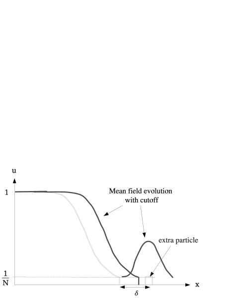
Figure 5: Evolution of the front with a forward fluctuation. At time $t_{0}$, the primary front extends over a size $L$ (Eq. (29)) and is a solution of the Brunet-Derrida cutoff equation (28). An extra particle has been stochastically generated at a distance $\delta$ with respect to the tip of the primary front. At a later time, the latter grows deterministically into a secondary front, that will add up to the primary one.

But it may happen that a few extra particles are sent stochastically ahead of the sharp tip of the front (See Fig. 5). Their evolution would pull the front forward. To model this effect, we assume that the probability per unit time that there be a particle sent at a distance $\delta$ ahead of the tip simply continues the asymptotic shape of the front, that is to say

$$p(\delta)=C_{1}e^{-\gamma_{0}\delta},$$ (31)

where $C_{1}$ is a constant. Heuristic arguments to support this assumption are presented in Ref. BDMM2005 (appendix A). Note that while the exponential shape is quite natural since it is the continuation of the deterministic solution (24), the fact that $C_{1}$ need to be strictly constant (and cannot be a slowly varying function of $\delta$) is a priori more difficult to argue.

Now once a particle has been produced at position $x_{\text{tip}}+\delta$, say at time $t_{0}$, it starts to multiply (see Fig. 5) and it eventually develops its own front (after a time of the order of $L^{2}$), that will add up to the deterministic primary front made of the evolution of the bulk of the particles.

Let us estimate the shift in the position of the front induced by these extra forward particles. Between the times $t_{0}$ and $t=t_{0}+L^{2}$, the velocity of the secondary front is given by Eq. (26). Hence its position $X_{t}^{(2)}$, after relaxation, will be given by

$$\begin{split}X_{t}^{(2)}&=X_{t}^{\text{BD}}+\delta+\int_{t_{0}}^{t}dt^{\prime}\,v_{t^{\prime}-t_{0}}\\ &\sim X_{t}^{\text{BD}}+\delta-\frac{3}{2\gamma_{0}}\ln L^{2}\end{split}$$ (32)

where $X_{t}^{\text{BD}}=V_{\text{BD}}t$. Eq. (32) holds up to a constant. We have used Eq. (26) to express $v_{t^{\prime}-t_{0}}$. The observed front will eventually result in the sum of the primary and secondary fronts, after relaxation of the latter. Its position will be $X_{t}^{\text{BD}}$ supplemented by a shift $R(\delta)$ that may be computed by writing the resulting front shape as the sum of the primary and secondary fronts:

$$e^{-\gamma_{0}(x-X_{t}^{\text{BD}}-R(\delta))}=e^{-\gamma_{0}(x-X_{t}^{\text{BD}})}\\ +C_{2}e^{-\gamma_{0}(x-X_{t}^{\text{BD}}-\delta+\frac{3}{2\gamma_{0}}\ln L^{2})},$$ (33)

where $C_{2}$ is an undetermined constant. From Eq. (33) we can compute the shift due to the relaxation of a forward fluctuation $R(\delta)$:

$$R(\delta)=\frac{1}{\gamma_{0}}\ln\left(1+C_{2}\frac{e^{\gamma_{0}\delta}}{L^{3}}\right).$$ (34)

The probability distribution (31) and the front shift (34) due to a forward fluctuation define an effective theory for the evolution of the position of the front $X_{t}$:

$$X_{t+dt}=\left\{\begin{aligned} &X_{t}+V_{\text{BD}}dt\ \ \text{proba}\ \ 1-p(\delta)d\delta dt\\ &X_{t}+V_{\text{BD}}dt+R(\delta)\ \ \text{proba}\ \ p(\delta)d\delta dt.\end{aligned}\right.$$ (35)

From these rules, we may compute all cumulants of $X_{t}$:

$$\begin{split}&V-V_{\text{BD}}=\int d\delta p(\delta)R(\delta)=\frac{C_{1}C_{2}}{\gamma_{0}}\frac{3\ln L}{\gamma_{0}L^{3}}\\ &\frac{[\text{$n$-th cumulant}]}{t}=\int d\delta p(\delta)[R(\delta)]^{n}\\ &\phantom{\frac{[\text{$n$-th cumulant}]}{t}}=\frac{C_{1}C_{2}}{\gamma_{0}}\frac{n!\zeta(n)}{\gamma_{0}^{n}L^{3}}.\end{split}$$ (36)

We see that the statistics of the position of the front still depend on the product $C_{1}C_{2}$ of the undetermined constants $C_{1}$ and $C_{2}$. We need a further assumption to fix its value.

We go back to the expression for the correction to the mean-field front velocity, given in Eq. (36). From the expressions of $R(\delta)$ (Eq. (34)) and of $p(\delta)$ (Eq. (31)), we see that the integrand defining $V-V_{\text{BD}}$ is almost a constant function of $\delta$ for $\delta<\delta_{0}=3\ln L/\gamma_{0}$, and is decaying exponentially for $\delta>\delta_{0}$. Furthermore, $R(\delta_{0})$ is of order 1, which means that when a fluctuation is emitted at a distance $\delta\sim\delta_{0}$ ahead of the tip of the front, it evolves into a front that matches in position the deterministic primary front. We also notice that when a fluctuation has $\delta<\delta_{0}$, its evolution is completely linear until it is incorporated to the primary front, whereas fluctuations with $\delta>\delta_{0}$ evolve nonlinearly but at the same time have a very suppressed probability. We are thus led to the natural conjecture that the average front velocity is given by Eq. (30), with the replacement $L\rightarrow\ln N/\gamma_{0}+\delta_{0}$. The large-$N$ expansion of the new expression of the velocity yields a correction of the order of $\ln\ln N/\ln^{3}N$ to the Brunet-Derrida result, more precisely

$$V=\frac{\chi(\gamma_{0})}{\gamma_{0}}-\frac{\pi^{2}\gamma_{0}\chi^{\prime\prime}(\gamma_{0})}{2\ln^{2}N}+\pi^{2}\gamma_{0}^{2}\chi^{\prime\prime}(\gamma_{0})\frac{3\ln\ln N}{\gamma_{0}\ln^{3}N}.$$ (37)

Eqs. (36) and (37) match for the choice $C_{1}C_{2}=\pi^{2}\chi^{\prime\prime}(\gamma_{0})$. From this determination of $C_{1}C_{2}$, we also get the full expression of the cumulants:

$$\frac{[\text{$n$-th cumulant}]}{t}=\pi^{2}\gamma_{0}^{2}\chi^{\prime\prime}(\gamma_{0})\frac{n!\zeta(n)}{\gamma_{0}^{n}\ln^{3}N}.$$ (38)

We note that all cumulants are of order unity for $t\sim\ln^{3}N$, which is the sign that the distribution of the front position is far from a trivial Gaussian, which makes it particularly interesting. On the other hand, they are proportional to $\kappa=t/\ln^{3}N$, which is the sign that the position of the front is the result of the sum of $\kappa$ independent random variables, and as such, becomes Gaussian when $\kappa$ is very large.

These results rely on a number of conjectures that no-one has been able to prove so far. However, we performed very precise numerical checks on specific models, and we found a perfect matching (see Ref. BDMM2005 ). So we are reasonably confident that our expressions are the correct ones. Providing a formal proof would be an interesting challenge for a mathematician.

The analytical results presented here, namely Eqs. (37) and (38), may directly be applied to QCD using the dictionary (18). This would help to improve the analytic form of the amplitude (17).

III.2 Traveling waves in evolution models

Let us now consider a model of population evolution. Each individual is characterized by a single real number $x$ that measures its adequacy to the environment. At time $t$, there are $n(t,x)$ individuals in the population with a given adequacy $x$. To go from time $t$ to $t+1$, we give the following rule: Each individual dies after having given birth to 2 offspring, that have respective adequacies $x+\varepsilon_{1}$ and $x+\varepsilon_{2}$, where $\varepsilon_{1,2}$ are random variables distributed according to a sufficiently local probability distribution $\psi$. If the total population exceeds a given integer $N$, then we get rid of the individuals with the lowest values of $x$ in order to keep the population size constant and equal to $N$. This model could represent for example the evolution of a population of bacterias under asexual reproduction, in a medium where resources are limited, which enforces a selection of the “best” individuals. Let us define $u(t,x)$ to be the fraction of population that has its adequacy variable larger than $x$. It is not difficult to realize that $u$ has the shape of a wave front, connecting a region where $u=1$ (for small values of $x$), and a region where $u=0$ (for larger values of $x$), that moves toward positive $x$ when time elapses, see Fig. 6.

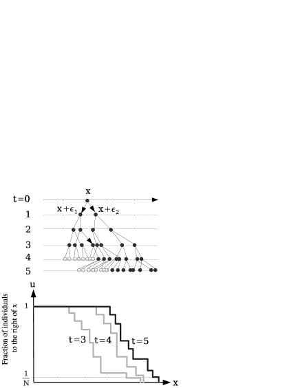
Figure 6: Evolution of the population over a few generations. In this model, each individual of a given generation $t$ has exactly two offspring, whose adequacy to environment differs from his by the random variables $\varepsilon_{1}$ and $\varepsilon_{2}$. Once the population size has reached $N$ ($N=8$ in this sketch), it is kept constant by allowing only the “best” $N$ individuals to have a descendance. The fraction $u$ of individuals having their adequacy variable larger than $x$ is plotted (bottom plot) for 3 different times. One sees that $u$ exhibits the characteristics of a traveling wave.

One may write a stochastic evolution equation for $u$:

$$u(t+1,x)=\min\left(1,2\int d\varepsilon\psi(\varepsilon)u(t,x-\varepsilon)\right)+\\ \sqrt{\frac{2}{N}\int d\varepsilon\psi(\varepsilon)u(t,x\!-\!\varepsilon)}\nu(t+1,x)$$ (39)

where as usually, $\nu$ is a noise of zero mean and variance of order 1 in the region where $u$ is small. At first sight, it is far from obvious that this equation should be in the universality class of the F-KPP equation. First, this is a finite difference equation in $t$ rather than a differential equation. Second, the noise term is non-Gaussian and furthermore, a closer look shows that $\nu$ is strongly correlated spatially. The nonlinearity is also of completely different nature in this model. However, the fact that a noisy front is formed for $u$ and especially the physical mechanism of evolution (branching diffusion+saturation) points toward the F-KPP universality class. If this is true, we can apply the results obtained in the previous subsection to study how the mean adequacy $x$ grows with time (this would be the average position of the front). It is easy to see that for this model, the characteristic function would be

$$\chi(\gamma)=\ln\left(2\int d\varepsilon\psi(\varepsilon)e^{\gamma\varepsilon}\right).$$ (40)

We checked that a numerical simulation of this model indeed matches the analytical predictions, confirming that the model (39) is indeed in the universality class defined by the F-KPP evolution.

For that kind of evolution models, one may ask a further question. At a given time $t$, one may pick a given number of individuals, say 2 or 3, and count the number of generations one has to go back in the past to find their most recent common ancestor. We denote these numbers by $T_{2}$, $T_{3}$…This question may be relevant to studies of the genetic diversity of a population.

Figure 7: Evolution of the population over a few generations. Each individual has two offspring in the next generation, but only the $N$ ($=8$ in this illustration) with highest values of $x$ are allowed to have a descendance. Sometimes, an individual is so advanced (it has to be ahead by at least $\delta=\delta_{0}=\frac{3}{\gamma_{0}}\ln\ln N$) that his descendance will take over the whole population. This happens, on the average, once in $\ln^{3}N$ generations. An estimator of this time scale may be obtained by picking 2, 3 or more individuals at random and looking for their common ancestor.

It is not difficult to guess the order of magnitude of $T_{i}$. We saw in the previous subsection that $X_{t}$ looked like the sum of $\kappa=t/\ln^{3}N$ independent random variables. One can understand this fact very precisely on this model. Indeed, from time to time, the evolution generates an individual whose adequacy to the environment is much larger than the one of any other individual. His offspring will partly inherit his adequacy, according to the stochastic evolution rules and thus will still be in advance with respect to the bulk of the population. After some generations, only his descendants may survive, so that he will be the common ancestor of the whole population. For an individual to have a significant probability to have his descendance replacing the whole population at some later time, the position of the secondary front developed by this individual has to be larger than the position of the primary front, a condition which reads $\delta>\ln L^{3}/\gamma_{0}$. According to Eq. (31), this happens once in $L^{3}=(\ln N/\gamma_{0})^{3}$ generations. Hence

$$T_{i}\sim\ln^{3}N.$$ (41)

It turns out that through a slightly more elaborate analysis, we may also fully compute the coefficients of the $T_{i}$, simply from the assumptions of the previous subsection on the mechanism of the propagation of the front. We found BDMM2006

$$\frac{\langle T_{3}\rangle}{\langle T_{2}\rangle}=\frac{5}{4},\ \ \ \frac{\langle T_{4}\rangle}{\langle T_{2}\rangle}=\frac{25}{18},\ \cdots$$ (42)

These numbers characterize the statistics of the genealogical trees that can be drawn in this kind of models.

It is not clear if results such as (41) and (42) may be applied to particle physics observables. The latter may be more relevant to evolutionary biology.

III.3 Spin glasses

A spin glass sg is a system of spins with random interactions. The Hamiltonian is given by Eq. (4), but the $J_{ij}$ are now random numbers endowed with a given probability distribution. The simplest case is when $J_{ij}$ are binary variables $\pm 1$, but the standard choice is a Gaussian distribution which leads to a model named after Edwards and Anderson. The Sherrington-Kirkpatrick model is the infinite-range version of the latter: The same distribution holds for any pair of spins and not only for nearest neighbors.

This time, the minimum energy state at zero temperature is not unique, contrarily to the Ising case for which the minimum energy configuration is reached when all spins are aligned. This is due to “frustration” (the fact that all interactions can never be satisfied simultaneously), and is illustrated in Fig. 8.

Figure 8: Two frustrated configurations of 4 spins, that have the same energy. The “$+$” and “$-$” on the lattice links represent the values of the interaction$J_{ij}$.

To classify the configurations, one may define the overlap between two spin configurations $a$ and $b$ as a function that reflects the fraction of spins that are common to $a$ and $b$. The usual definition is $q_{ab}=\frac{1}{N}\sum_{i}S_{i}^{a}S_{i}^{b}$. Speaking through the hat, the configurations that minimize the energy are organized ultrametrically with respect to a distance derived from the overlap. This means that the configurations may be represented as the leaves of a (random) tree. The statistics of this tree, first found by Parisi sg2 , turn out to be exactly the same as the ones of our genealogic trees in the previous subsection that are encoded in the ratios (42).

It should be clear to the reader that there is no a priori reason for such a feature. The method for finding the statistics in Parisi’s theory relies on the replica method (see Ref. BDMM2006 for details), and has nothing to do with the way we derived the result in our case. Whether this link is deep or accidental is an outstanding open question, for which we have no clue.

IV Conclusion

When it was first suggested that high energy QCD has something to do with reaction-diffusion processes and that this analogy leads to new quantitative predictions M2004 , many experts were skeptical and reluctant to accept this new point of view. Getting these ideas through has involved some passionate debates, to say the least. But at the time of the present lectures, that is two years later, this proposal has undoubiously triggered a burst of activity, that has spread in many different directions.

The main advantage of viewing high energy scattering in the peculiar way that we have explained here is that it provides a simple picture endowed with a clear physical interpretation. This contrasts with the high technicity of evolution equations for QCD amplitudes that had been derived over the last 10 years such as the Balitsky hierarchy (2). Furthermore, this picture has a direct and intuitive connection with the basics of the parton model. This approach has paved the way for new results in QCD, obtained from tools known in statistical physics.

Obviously, there is still room for improvements of our understanding of high energy scattering. Admittedly, our proposal relies on a few conjectures that will have to be proved. In our opinion, the most problematic one is the assumption that the number of gluons or of color dipoles saturates at $1/\alpha_{s}^{2}$ per unit of transverse phase space. Of course, this has been part of the “folklore” of high energy physics at least since the seminal work of Gribov, Levin, Ryskin in the 80’s GLRMQ . However, no QCD realization of saturation has yet been found. A relevant question would be, for example, how parton recombination may be implemented in the framework of the color dipole model. Some interesting ideas have recently been put forward (see e.g. Ref. AGL ), but a rigorous proof in QCD still has to be provided.

In the second lecture, we have presented some recent advances in statistical physics to which we have been able to contribute. Here also, there is an intriguing correspondence between two seemingly different physical problems: stochastic fronts and the theory of spin glasses. Whether this is something deep or simply accidental still remains to be understood.

- (1) I. Balitsky, Nucl. Phys.B463 (1996) 99; Phys. Rev. Lett. 81 (1998) 2024; Phys. Lett. B518 (2001) 235.
- (2) Y.V. Kovchegov, Phys. Rev. D60 (1999) 034008; Phys. Rev. D61 (2000) 074018.
- (3) E. Levin and K. Tuchin, Nucl. Phys. B 573, 833 (2000).
- (4) A. H. Mueller and D. N. Triantafyllopoulos, Nucl. Phys. B 640, 331 (2002).
- (5) S. Munier and R. Peschanski, Phys. Rev. Lett. 91 (2003) 232001; Phys. Rev. D69 (2004) 034008.
- (6) S. Munier and R. Peschanski, Phys. Rev. D 70, 077503 (2004).
- (7) L.V. Gribov, E.M. Levin and M. G. Ryskin, Phys. Rep. 100 (1983) 1; A. H. Mueller and J. w. Qiu, Nucl. Phys. B 268, 427 (1986).
- (8) L. N. Lipatov, Sov. J. Nucl. Phys. 23, 338 (1976); E. A. Kuraev, L. N. Lipatov, and V. S. Fadin, Sov. Phys. JETP 45, 199 (1977); I. I. Balitsky and L. N. Lipatov, Sov. J. Nucl. Phys. 28, 822 (1978).
- (9) K. Golec-Biernat and M. Wüsthoff, Phys. Rev. D 59, 014017 (1999); Phys. Rev. D 60, 114023 (1999).
- (10) S. Munier, A. M. Staśto and A. H. Mueller, Nucl. Phys. B 603, 427 (2001).
- (11) A. H. Mueller and A. I. Shoshi, Nucl. Phys. B 692 (2004) 175.
- (12) S. Munier, Proceedings of the Theory Summer Program on RHIC physics, BNL-73263-2004, Brookhaven, July 2004.
- (13) E. Iancu, A. H. Mueller and S. Munier, Phys. Lett. B 606, 342 (2005); S. Munier, Nucl. Phys. A 755, 622 (2005).
- (14) R. Enberg, K. Golec-Biernat and S. Munier, Phys. Rev. D 72, 074021 (2005).
- (15) S. Munier, Phys. Rev. D 75 034009 (2007).
- (16) A. I. Shoshi and B. W. Xiao, Phys. Rev. D 73, 094014 (2006).
- (17) R. A. Fisher, Ann. Eugenics 7, 355 (1937); A. Kolmogorov, I. Petrovsky, and N. Piscounov, Moscou Univ. Bull. Math. A1, 1 (1937).
- (18) For a recent review on stochastic fronts, see D. Panja, Phys. Rept. 393 (2004) 87.
- (19) E. Brunet and B. Derrida, Phys. Rev. E56 (1997) 2597; Comp. Phys. Comm. 121-122 (1999) 376; J. Stat. Phys. 103 (2001) 269.
- (20) A. H. Mueller, Nucl. Phys. B 415 (1994) 373.
- (21) A. M. Staśto, K. Golec-Biernat and J. Kwieciński, Phys. Rev. Lett. 86 (2001) 596.
- (22) E. Brunet, B. Derrida, A. H. Mueller and S. Munier, Phys. Rev. E 73, 056126 (2006).
- (23) E. Brunet, B. Derrida, A. H. Mueller and S. Munier, Europhys. Lett. 76, 1 (2006); extended version in preparation.
- (24) For a review on experimental and theoretical aspects of spin glasses, see e.g. K. Binder, A. P. Young, Rev. Mod. Phys. 58, 801 (1986).
- (25) G. Parisi, J. Phys. A 13, 1101 (1980); M. Mézard , G. Parisi, N. Sourlas, G. Toulouse, M. A. Virasoro, Journal de Physique 45, 843-854 (1984).
- (26) E. Avsar, G. Gustafson and L. Lonnblad, JHEP 0507, 062 (2005).