Abstract

In this work, we study the four form-factors $f_{1}(Q^{2})$, $f_{2}(Q^{2})$, $g_{1}(Q^{2})$ and $g_{2}(Q^{2})$ of the $\Sigma\to n$ in the framework of the light-cone QCD sum rules approach up to twist-6 three valence quark light-cone distribution amplitudes. The $f_{1}(0)$ is the basic input parameter in extracting the CKM matrix element $|V_{us}|$ from the hyperon decays. The four form-factors $f_{1}(Q^{2})$, $f_{2}(Q^{2})$, $g_{1}(Q^{2})$ and $g_{2}(Q^{2})$ at intermediate and large momentum transfers with $Q^{2}>3GeV^{2}$ have significant contributions from the end-point (soft) terms. The numerical values of the four form-factors $f_{1}(0)$, $f_{2}(0)$, $g_{1}(0)$ and $g_{2}(0)$ are compatible with the experimental data and theoretical calculations (in magnitude); although the uncertainties are large.

PACS numbers: 12.38.Lg; 12.38.Bx; 12.15.Hh

Key Words: Form-factors, CKM matrix element, light-cone QCD sum rules

1 Introduction

Semileptonic decays $K\to\pi\ell\nu$ ($K_{\ell 3}$) provide the most precise determination of the Cabibbo-Kobayashi-Maskawa (CKM) matrix element $|V_{us}|$ [1]. The experimental input parameters are the semileptonic decay widths and the vector form-factors $f^{+}_{K\pi}(q^{2})$ and $f^{-}_{K\pi}(q^{2})$, which are necessary in calculating the phase space integrals. The main uncertainty in the quantity $|V_{us}f^{+}_{K\pi}(0)|$ comes from the unknown shape of the hadronic form-factor $f^{+}_{K\pi}(q^{2})$, which is measurable at $m_{l}^{2}<q^{2}<(m_{K}-m_{\pi})^{2}$ in the $K_{\ell 3}$ decays or $(m_{K}+m_{\pi})^{2}<q^{2}<m^{2}_{\tau}$ in the $\tau\to K\pi\nu$ decays. Another way to extract the $|V_{us}|$ is provided by the hyperon semileptonic decays, it is possible to extract the quantity $|V_{us}f_{1}(0)|$ at the percent level from the hyperon experiments [2], where the $f_{1}(0)$ is the vector form-factor at zero-momentum transfer. The Ademollo-Gatto theorem protects the $f_{1}(0)$ from the first-order $SU(3)$-breaking corrections [3], while the second-order corrections are badly known. There exist several model dependent estimates for the $f_{1}(0)$, for examples, quark models [4], large-$N_{c}$ [5] and chiral expansions[6]; however, the values disagree with each other. The axial-vector form-factor $g_{1}(0)$ is not protected by the Ademollo-Gatto theorem, and it suffers from the first-order $SU(3)$ breaking corrections. The $SU(3)$ symmetry implies a vanishing ”weak-electricity” form-factor $g_{2}(Q^{2})$, because charge conjugation does not allow a $C$-odd term $g_{2}(Q^{2})$ in the matrix elements of the neutral axial-vector currents $A_{\mu}^{3}$ and $A_{\mu}^{8}$, which are $C$-even.

In our previously work, we study the vector form-factors $f^{+}_{K\pi}(q^{2})$ and $f^{-}_{K\pi}(q^{2})$ with the light-cone QCD sum rules (LCSR), and obtain satisfactory results [7]. In this article, we calculate the four form-factors $f_{1}(Q^{2})$, $f_{2}(Q^{2})$, $g_{1}(Q^{2})$ and $g_{2}(Q^{2})$ of the $\Sigma\to n$ in the framework of the LCSR approach [8, 9], which combine the standard techniques of the QCD sum rules with the conventional parton distribution amplitudes describing the hard exclusive processes[10]. In the LCSR approach, the short-distance operator product expansion with the vacuum condensates of increasing dimensions is replaced by the light-cone expansion with the distribution amplitudes (which correspond to the sum of an infinite series of operators with the same twist) of increasing twists to parameterize the non-perturbative QCD vacuum. The higher twists light-cone distribution amplitudes of the baryons were not available until recently [11], then the LCSRs were applied to study the form-factors of the nucleons [12, 13, 14] and the weak decays [15].

The article is arranged as: in Section 2, we derive the analytical expressions of the four form-factors $f_{1}(Q^{2})$, $f_{2}(Q^{2})$, $g_{1}(Q^{2})$ and $g_{2}(Q^{2})$ with the light-cone QCD sum rules approach; in Section 3, the numerical results and discussions; and in Section 4, conclusion.

2 Form-factors $f_{1}(Q^{2})$, $f_{2}(Q^{2})$, $g_{1}(Q^{2})$ and $g_{2}(Q^{2})$ with light-cone QCD sum rules

In the following, we write down the two-point correlation function $\Pi_{\mu}(P,q)$ in the framework of the LCSR approach,

$$\Pi_{\mu}(P,q) = i\int d^{4}x\,e^{-iq\cdot x}\langle 0|T\left\{\eta(0)J_{\mu}(x)\right\}|P\rangle,$$ (1)

with the chiral current

$$J_{\mu}(x) = \bar{s}(x)\gamma_{\mu}(1-\gamma_{5})u(x),$$ (2)

and the Ioffe current for the $\Sigma$ baryon [16]

$$\eta(0) = \epsilon^{abc}d^{T}_{a}(0)C\gamma_{\mu}d_{b}(0)\,\gamma_{5}\gamma^{\mu}s_{c}(0)\,,$$

$$\langle 0|\eta(0)|P\rangle = \lambda_{\Sigma}N(P)\,,$$ (3)

here the $\lambda_{\Sigma}$ is the coupling constant of the $\Sigma$ baryon. There are two independent interpolating currents with the spin-$\frac{1}{2}$ and isospin-1, both are expected to excite the ground state $\Sigma$ baryon from the vacuum, the general form of the $\Sigma$ current can be written as [17]

$$\eta(x,t) = \epsilon^{abc}\left\{d_{a}^{T}(x)Cs_{b}(x)\gamma_{5}d_{c}(x)+td_{a}^{T}(x)C\gamma_{5}s_{b}(x)d_{c}(x)\right\},$$

in the limit $t=-1$, the Ioffe current is recovered, we can take the $t$ as a free parameter and select the ideal value with the QCD sum rules approach, here we prefer the Ioffe current $\eta(x)$ to keep in consistent with the QCD sum rules used in determining the parameters in the light-cone distribution amplitudes. We can also choose the Chernyak-Zhitnitsky type current to interpolate the $\Sigma$ baryon [18]

$$\eta(x) = \epsilon^{abc}d^{T}_{a}(x)C\!\not\!{z}d_{b}(x)\,\gamma_{5}\!\not\!{z}s_{c}(x)\,,$$

where the $z_{\mu}$ is a light-cone four-vector, the currents of this type have non-vanishing couplings to both the spin-$\frac{1}{2}$ and -$\frac{3}{2}$ baryon states, it is difficult to separate the contribution of the spin-$\frac{3}{2}$ state.

At the large Euclidean momenta ${P^{\prime}}^{2}=(P+q)^{2}$ and $q^{2}=-Q^{2}$, the correlation function $\Pi_{\mu}(P,q)$ can be calculated in perturbation theory. In calculation, we need the following light-cone expanded quark propagator [19],

$$S(x) = \frac{i\not\!x}{2\pi^{2}x^{4}}-\frac{m}{4\pi^{2}x^{2}}$$ (4)

$$- \frac{i}{16\pi^{2}x^{2}}\int\limits_{0}^{1}dv\Big{\{}(1-v)\not\!x\sigma_{\mu\nu}G^{\mu\nu}(vx)+v\sigma_{\mu\nu}G^{\mu\nu}(vx)\!\not\!x\Big{\}}+...,$$

where $G_{\mu\nu}=g_{s}G_{\mu\nu}^{a}(\lambda^{a}/2)$ is the gluon field strength tensor. The contributions proportional to the $G_{\mu\nu}$ can give rise to four-particle (and five-particle) nucleon distribution amplitudes with a gluon (or quark-antiquark pair) in addition to the three valence quarks, their corrections are usually not expected to play any significant roles [20] and neglected here [12, 13, 15]. In the parton model, at large momentum transfers, the electromagnetic and weak currents interact with the almost free partons in the nucleons. Employ the ”free” light-cone quark propagator in the correlation function $\Pi_{\mu}(P,q)$, we obtain

$$z^{\mu}\Pi_{\mu}(P,q)$$

$$= \int d^{4}x\,\frac{e^{-iq\cdot x}}{2\pi^{2}x^{4}}(C\gamma_{\mu})^{\alpha\beta}\left[\gamma^{\mu}\!\not\!{x}\!\not\!{z}(1-\gamma_{5})\right]^{\eta\lambda}\epsilon_{ijk}\langle 0|T\left\{d^{i}_{\alpha}(0)d^{j}_{\beta}(0)u^{k}_{\lambda}(x)\right\}|P\rangle$$

$$+ m_{s}i\int d^{4}x\,\frac{e^{-iq\cdot x}}{4\pi^{2}x^{2}}(C\gamma_{\mu})^{\alpha\beta}\left[\gamma^{\mu}\!\not\!{z}(1-\gamma_{5})\right]^{\eta\lambda}\epsilon_{ijk}\langle 0|T\left\{d^{i}_{\alpha}(0)d^{j}_{\beta}(0)u^{k}_{\lambda}(x)\right\}|P\rangle.$$

In the light-cone limit $x^{2}\to 0$, the remaining three-quark operator sandwiched between the neutron state $|P\rangle$ and the vacuum can be written in terms of the nucleon distribution amplitudes [11, 18, 21]. The three valence quark components of the nucleon distribution amplitudes are defined by the matrix element,

$$4\langle 0|\epsilon_{ijk}d_{\alpha}^{i}(a_{1}x)d_{\beta}^{j}(a_{2}x)u_{\gamma}^{k}(a_{3}x)|P\rangle=(\mathcal{V}_{1}+\frac{x^{2}M_{n}^{2}}{4}\mathcal{V}_{1}^{M})(\hbox to0.0pt{/\hss}PC)_{\alpha\beta}(\gamma_{5}N)_{\gamma}$$

$${}+\mathcal{V}_{2}M_{n}(\hbox to0.0pt{/\hss}PC)_{\alpha\beta}(\hbox to0.0pt{/\hss}x\gamma_{5}N)_{\gamma}+\mathcal{V}_{3}M_{n}(\gamma_{\mu}C)_{\alpha\beta}(\gamma^{\mu}\gamma_{5}N)_{\gamma}+\mathcal{V}_{4}M_{n}^{2}(\hbox to0.0pt{/\hss}xC)_{\alpha\beta}(\gamma_{5}N)_{\gamma}$$

$${}+\mathcal{V}_{5}M_{n}^{2}(\gamma_{\mu}C)_{\alpha\beta}(i\sigma^{\mu\nu}x_{\nu}\gamma_{5}N)_{\gamma}+\mathcal{V}_{6}M_{n}^{3}(\hbox to0.0pt{/\hss}xC)_{\alpha\beta}(\hbox to0.0pt{/\hss}x\gamma_{5}N)_{\gamma}+\cdots.$$ (5)

The calligraphic distribution amplitudes do not have definite twist and can be related to the ones with definite twist as

$$\mathcal{V}_{1}=V_{1},\hskip 68.28644pt2P\cdot x\mathcal{V}_{2}=V_{1}-V_{2}-V_{3},$$

$$2\mathcal{V}_{3}=V_{3},\hskip 62.59596pt4P\cdot x\mathcal{V}_{4}=-2V_{1}+V_{3}+V_{4}+2V_{5},$$

$$4P\cdot x\mathcal{V}_{5}=V_{4}-V_{3},\hskip 14.22636pt(2P\cdot x)^{2}\mathcal{V}_{6}=-V_{1}+V_{2}+V_{3}+V_{4}+V_{5}-V_{6}$$

for the vector distribution amplitudes. The light-cone distribution amplitudes $F=V_{i}$ can be represented as

$$F(a_{i}p\cdot x)=\int dx_{1}dx_{2}dx_{3}\delta(x_{1}+x_{2}+x_{3}-1)e^{-ip\cdot x\Sigma_{i}x_{i}a_{i}}F(x_{i})\,.$$ (6)

The distribution amplitudes are scale dependent and can be expanded with the operators of increasing conformal spin, we write down the explicit expressions for the $V_{i}$ up to the next-to-leading conformal spin accuracy in the appendix [11]. The $V_{1}$ is the leading twist-3 distribution amplitude; the $V_{2}$ and $V_{3}$ are the twist-4 distribution amplitudes; the $V_{4}$ and $V_{5}$ are the twist-5 distribution amplitudes; while the twist-6 distribution amplitude is the $V_{6}$. The parameters $\phi_{3}^{0}$, $\phi_{6}^{0}$, $\phi_{4}^{0}$, $\phi_{5}^{0}$, $\xi_{4}^{0}$, $\xi_{5}^{0}$, $\psi_{4}^{0}$, $\psi_{5}^{0}$, $\phi_{3}^{-}$, $\phi_{3}^{+}$, $\phi_{4}^{-}$, $\phi_{4}^{+}$, $\psi_{4}^{-}$, $\psi_{4}^{+}$, $\xi_{4}^{-}$, $\xi_{4}^{+}$, $\phi_{5}^{-}$, $\phi_{5}^{+}$, $\psi_{5}^{-}$, $\psi_{5}^{+}$, $\xi_{5}^{-}$, $\xi_{5}^{+}$, $\phi_{6}^{-}$, $\phi_{6}^{+}$ in the light-cone distribution amplitudes $V_{i}$ can be expressed in terms of eight independent matrix elements of the local operators with the parameters $f_{N}$, $\lambda_{1}$, $\lambda_{2}$, $V_{1}^{d}$, $A_{1}^{u}$, $f^{d}_{1}$, $f^{d}_{2}$ and $f^{u}_{1}$, the three parameters $f_{N}$, $\lambda_{1}$ and $\lambda_{2}$ are related to the leading order (or $S$-wave) contributions of the conformal spin expansion, the remaining five parameters $V_{1}^{d}$, $A_{1}^{u}$, $f^{d}_{1}$, $f^{d}_{2}$ and $f^{u}_{1}$ are related to the next-to-leading order (or $P$-wave) contributions of the conformal spin expansion; the explicit expressions are given in the appendix; for the details, one can consult Ref.[11].

Taking into account the three valence quark light-cone distribution amplitudes up to twist-6 and performing the integration over the $x$ in the coordinate space, finally we obtain the following results,

$$z^{\mu}\Pi_{\mu}(P,q)$$ (7)

$$= 2P\cdot zN(P)\left\{\int_{0}^{1}dt_{3}\int_{0}^{1-t_{3}}dt_{1}\frac{M_{n}V_{3}t_{3}+m_{s}V_{1}}{(q+t_{3}P)^{2}}\right.$$

$$+M_{n}\int_{0}^{1}d\lambda\int_{1}^{\lambda}dt_{3}\int_{0}^{1-t_{3}}dt_{1}\frac{2q\cdot P\lambda(V_{1}-V_{2}-V_{3})+\lambda^{2}M_{n}^{2}(V_{1}-V_{2}-2V_{3}+V_{4})}{(q+\lambda P)^{4}}$$

$$\left.+M_{n}^{2}m_{s}\int_{0}^{1}d\lambda\lambda\int_{1}^{\lambda}dt_{3}\int_{0}^{1-t_{3}}dt_{1}\frac{-2V_{1}+V_{2}+V_{3}+V_{4}+V_{5}}{(q+\lambda P)^{4}}\right\}$$

$$+ 2P\cdot z\!\not\!qN(P)\left\{\int_{0}^{1}dt_{3}\int_{0}^{1-t_{3}}dt_{1}\left[\frac{V_{1}}{(q+t_{3}P)^{2}}+\frac{M_{n}^{2}V_{1}^{M}}{(q+t_{3}P)^{4}}\right]\right.$$

$$\left.-M_{n}\int_{0}^{1}d\lambda\int_{1}^{\lambda}dt_{3}\int_{0}^{1-t_{3}}dt_{1}\frac{M_{n}\lambda(V_{1}-V_{2}-V_{4})+m_{s}(V_{1}-V_{2}-V_{3})}{(q+\lambda P)^{4}}\right\}$$

$$+ 2P\cdot z\gamma_{5}N(P)\left\{\int_{0}^{1}dt_{3}\int_{0}^{1-t_{3}}dt_{1}\frac{M_{n}V_{3}t_{3}-m_{s}V_{1}}{(q+t_{3}P)^{2}}\right.$$

$$+M_{n}\int_{0}^{1}d\lambda\int_{1}^{\lambda}dt_{3}\int_{0}^{1-t_{3}}dt_{1}\frac{2q\cdot P\lambda(V_{1}-V_{2}-V_{3})+\lambda^{2}M_{n}^{2}(V_{1}-V_{2}-2V_{3}+V_{4})}{(q+\lambda P)^{4}}$$

$$\left.-M_{n}^{2}m_{s}\int_{0}^{1}d\lambda\lambda\int_{1}^{\lambda}dt_{3}\int_{0}^{1-t_{3}}dt_{1}\frac{-2V_{1}+V_{2}+V_{3}+V_{4}+V_{5}}{(q+\lambda P)^{4}}\right\}$$

$$- 2P\cdot z\!\not\!q\gamma_{5}N(P)\left\{\int_{0}^{1}dt_{3}\int_{0}^{1-t_{3}}dt_{1}\left[\frac{V_{1}}{(q+t_{3}P)^{2}}+\frac{M_{n}^{2}V_{1}^{M}}{(q+t_{3}P)^{4}}\right]\right.$$

$$\left.-M_{n}\int_{0}^{1}d\lambda\int_{1}^{\lambda}dt_{3}\int_{0}^{1-t_{3}}dt_{1}\frac{M_{n}\lambda(V_{1}-V_{2}-V_{4})-m_{s}(V_{1}-V_{2}-V_{3})}{(q+\lambda P)^{4}}\right\}$$

$$+ \cdots,$$

here the $V_{i}=V_{i}(t_{1},t_{2},t_{3})$.

According to the basic assumption of current-hadron duality in the QCD sum rules approach [10], we insert a complete series of intermediate states satisfying the unitarity principle with the same quantum numbers as the current operator $\eta(0)$ into the correlation function in Eq.(1) to obtain the hadronic representation. After isolating the pole term of the lowest $\Sigma$ state, we obtain the following result,

$$z^{\mu}\Pi_{\mu}(P,q) = \frac{\lambda_{\Sigma}N(P^{\prime})\langle N(P^{\prime})|\bar{s}(0)\!\not\!{z}(1-\gamma_{5})u(0)|N(P)\rangle}{M_{\Sigma}^{2}-(q+P)^{2}}+\cdots$$ (8)

$$= 2P\cdot z\lambda_{\Sigma}\frac{f_{1}+g_{1}\gamma_{5}}{M_{\Sigma}^{2}-(q+P)^{2}}N(P)+$$

$$2P\cdot z\frac{\lambda_{\Sigma}}{M_{n}+M_{\Sigma}}\frac{f_{2}\!\not\!{q}+g_{2}\!\not\!{q}\gamma_{5}}{M_{\Sigma}^{2}-(q+P)^{2}}N(P)+\cdots\,.$$

here we have used the definition,

$$\langle N(P^{\prime})|\bar{s}(0)\!\not\!{z}(1-\gamma_{5})u(0)|N(P)\rangle$$ (9)

$$= N(P^{\prime})\left\{\!\not\!{z}f_{1}-i\frac{z_{\mu}\sigma^{\mu\nu}q_{\nu}}{M_{\Sigma}+M_{n}}f_{2}+\frac{q\cdot z}{M_{\Sigma}+M_{n}}f_{3}\right\}N(P)+$$

$$N(P^{\prime})\left\{\!\not\!{z}g_{1}-i\frac{z_{\mu}\sigma^{\mu\nu}q_{\nu}}{M_{\Sigma}+M_{n}}g_{2}+\frac{q\cdot z}{M_{\Sigma}+M_{n}}g_{3}\right\}\gamma_{5}N(P)\,.$$

Here we choose the light-cone four vector $z_{\mu}$ with $q\cdot z=0$ and $z^{2}=0$. The tensor structures $2P\cdot z$, $2P\cdot z\gamma_{5}$, $2P\cdot z\!\not\!{q}$ and $2P\cdot z\!\not\!{q}\gamma_{5}$ are chosen to analyze the four form-factors $f_{1}(Q^{2})$, $f_{2}(Q^{2})$, $g_{1}(Q^{2})$ and $g_{2}(Q^{2})$, respectively.

The Borel transformation and the continuum states subtraction can be performed by using the following substitution rules,

$$\int dx\frac{\rho(x)}{(q+xP)^{2}} = -\int_{0}^{1}\frac{dx}{x}\frac{\rho(x)}{s-{P^{\prime}}^{2}}\Rightarrow-\int_{x_{0}}^{1}\frac{dx}{x}\rho(x)e^{-\frac{s}{M_{B}^{2}}},$$

$$\int dx\frac{\rho(x)}{(q+xP)^{4}} = \int_{0}^{1}\frac{dx}{x^{2}}\frac{\rho(x)}{(s-{P^{\prime}}^{2})^{2}}\Rightarrow\frac{1}{M_{B}^{2}}\int_{x_{0}}^{1}\frac{dx}{x^{2}}\rho(x)e^{-\frac{s}{M_{B}^{2}}}+\frac{\rho(x_{0})e^{-\frac{s_{0}}{M_{B}^{2}}}}{Q^{2}+x_{0}^{2}M_{n}^{2}}\,,$$

$$s = (1-x)M_{n}^{2}+\frac{(1-x)}{x}Q^{2},$$

$$x_{0} = \frac{\sqrt{(Q^{2}+s_{0}-M_{n}^{2})^{2}+4M_{n}^{2}Q^{2}}-(Q^{2}+s_{0}-M_{n}^{2})}{2M_{n}^{2}}.$$ (10)

Matching the hadronic representations and the corresponding representations at the level of the quark-gluons degrees of freedom below the threshold $s_{0}$, we obtain the sum rules for the four form-factors $f_{1}(Q^{2})$, $f_{2}(Q^{2})$, $g_{1}(Q^{2})$ and $g_{2}(Q^{2})$ ,

$$f_{1}(Q^{2})\lambda_{\Sigma}e^{-\frac{M_{\Sigma}^{2}}{M_{B}^{2}}}$$ (11)

$$= -\int_{x_{0}}^{1}dt_{3}\int_{0}^{1-t_{3}}dt_{1}\exp\left\{-\frac{t_{3}(1-t_{3})M_{n}^{2}+(1-t_{3})Q^{2}}{t_{3}M_{B}^{2}}\right\}\left[M_{n}V_{3}+\frac{m_{s}V_{1}}{t_{3}}\right]$$

$$+ x_{0}M_{n}^{2}\int_{x_{0}}^{1}dt_{3}\int_{0}^{1-t_{3}}dt_{1}\exp\left\{-\frac{s_{0}}{M_{B}^{2}}\right\}$$

$$\frac{x_{0}M_{n}(V_{1}-V_{2}-V_{4})-m_{s}(-2V_{1}+V_{2}+V_{3}+V_{4}+V_{5})}{x_{0}^{2}M_{n}^{2}+Q^{2}}$$

$$- \frac{M_{n}^{2}}{M_{B}^{2}}\int_{x_{0}}^{1}d\lambda\int_{1}^{\lambda}dt_{2}\int_{0}^{1-t_{2}}dt_{1}\frac{1}{\lambda}\exp\left\{-\frac{\lambda(1-\lambda)M^{2}+(1-\lambda)Q^{2}}{\lambda M_{B}^{2}}\right\}$$

$$\left[M_{n}\lambda(V_{1}-V_{2}-V_{4})-m_{s}(-2V_{1}+V_{2}+V_{3}+V_{4}+V_{5})\right]$$

$$+ M_{n}\int_{x_{0}}^{1}d\lambda\int_{1}^{\lambda}dt_{2}\int_{0}^{1-t_{2}}dt_{1}(V_{1}-V_{2}-V_{3})\lambda$$

$$\frac{d}{d\lambda}\frac{1}{\lambda}\exp\left\{-\frac{\lambda(1-\lambda)M^{2}+(1-\lambda)Q^{2}}{\lambda M_{B}^{2}}\right\}\,;$$

$$g_{1}(Q^{2})\lambda_{\Sigma}e^{-\frac{M_{\Sigma}^{2}}{M_{B}^{2}}}$$ (12)

$$= -\int_{x_{0}}^{1}dt_{3}\int_{0}^{1-t_{3}}dt_{1}\exp\left\{-\frac{t_{3}(1-t_{3})M_{n}^{2}+(1-t_{3})Q^{2}}{t_{3}M_{B}^{2}}\right\}\left[M_{n}V_{3}-\frac{m_{s}V_{1}}{t_{3}}\right]$$

$$+ x_{0}M_{n}^{2}\int_{x_{0}}^{1}dt_{3}\int_{0}^{1-t_{3}}dt_{1}\exp\left\{-\frac{s_{0}}{M_{B}^{2}}\right\}$$

$$\frac{x_{0}M_{n}(V_{1}-V_{2}-V_{4})+m_{s}(-2V_{1}+V_{2}+V_{3}+V_{4}+V_{5})}{x_{0}^{2}M_{n}^{2}+Q^{2}}$$

$$- \frac{M_{n}^{2}}{M_{B}^{2}}\int_{x_{0}}^{1}d\lambda\int_{1}^{\lambda}dt_{2}\int_{0}^{1-t_{2}}dt_{1}\frac{1}{\lambda}\exp\left\{-\frac{\lambda(1-\lambda)M^{2}+(1-\lambda)Q^{2}}{\lambda M_{B}^{2}}\right\}$$

$$\left[\lambda M_{n}(V_{1}-V_{2}-V_{4})+m_{s}(-2V_{1}+V_{2}+V_{3}+V_{4}+V_{5})\right]$$

$$+ M_{n}\int_{x_{0}}^{1}d\lambda\int_{1}^{\lambda}dt_{2}\int_{0}^{1-t_{2}}dt_{1}(V_{1}-V_{2}-V_{3})\lambda$$

$$\frac{d}{d\lambda}\frac{1}{\lambda}\exp\left\{-\frac{\lambda(1-\lambda)M^{2}+(1-\lambda)Q^{2}}{\lambda M_{B}^{2}}\right\}\,;$$

$$f_{2}(Q^{2})\frac{\lambda_{\Sigma}}{M_{\Sigma}+M_{n}}e^{-\frac{M_{\Sigma}^{2}}{M_{B}^{2}}}$$ (13)

$$= -\int_{x_{0}}^{1}dt_{3}\int_{0}^{1-t_{3}}dt_{1}\exp\left\{-\frac{t_{3}(1-t_{3})M_{n}^{2}+(1-t_{3})Q^{2}}{t_{3}M_{B}^{2}}\right\}\left[\frac{V_{1}}{t_{3}}-\frac{M_{n}^{2}V_{1}^{M}}{t_{3}^{2}M_{B}^{2}}\right]$$

$$+ M_{n}\int_{x_{0}}^{1}dt_{3}\int_{0}^{1-t_{3}}dt_{1}\exp\left\{-\frac{s_{0}}{M_{B}^{2}}\right\}\frac{x_{0}M_{n}(V_{1}-V_{2}-V_{4})+m_{s}(V_{1}-V_{2}-V_{3})}{x_{0}^{2}M_{n}^{2}+Q^{2}}$$

$$- \frac{M_{n}}{M_{B}^{2}}\int_{x_{0}}^{1}d\lambda\int_{1}^{\lambda}dt_{2}\int_{0}^{1-t_{2}}dt_{1}\exp\left\{-\frac{\lambda(1-\lambda)M^{2}+(1-\lambda)Q^{2}}{\lambda M_{B}^{2}}\right\}$$

$$\frac{\lambda M_{n}(V_{1}-V_{2}-V_{4})+m_{s}(V_{1}-V_{2}-V_{3})}{\lambda^{2}}$$

$$+ M_{n}^{2}\int_{0}^{1-x_{0}}dt_{1}\frac{V_{1}^{M}}{x_{0}^{2}M_{n}^{2}+Q^{2}}\exp\left\{-\frac{s_{0}}{M_{B}^{2}}\right\}\,;$$

$$g_{2}(Q^{2})\frac{\lambda_{\Sigma}}{M_{\Sigma}+M_{n}}e^{-\frac{M_{\Sigma}^{2}}{M_{B}^{2}}}$$ (14)

$$= \int_{x_{0}}^{1}dt_{3}\int_{0}^{1-t_{3}}dt_{1}\exp\left\{-\frac{t_{3}(1-t_{3})M_{n}^{2}+(1-t_{3})Q^{2}}{t_{3}M_{B}^{2}}\right\}\left[\frac{V_{1}}{t_{3}}-\frac{M_{n}^{2}V_{1}^{M}}{t_{3}^{2}M_{B}^{2}}\right]$$

$$- M_{n}\int_{x_{0}}^{1}dt_{3}\int_{0}^{1-t_{3}}dt_{1}\exp\left\{-\frac{s_{0}}{M_{B}^{2}}\right\}\frac{x_{0}M_{n}(V_{1}-V_{2}-V_{4})-m_{s}(V_{1}-V_{2}-V_{3})}{x_{0}^{2}M_{n}^{2}+Q^{2}}$$

$$+ \frac{M_{n}}{M_{B}^{2}}\int_{x_{0}}^{1}d\lambda\int_{1}^{\lambda}dt_{2}\int_{0}^{1-t_{2}}dt_{1}\exp\left\{-\frac{\lambda(1-\lambda)M^{2}+(1-\lambda)Q^{2}}{\lambda M_{B}^{2}}\right\}$$

$$\frac{\lambda M_{n}(V_{1}-V_{2}-V_{4})-m_{s}(V_{1}-V_{2}-V_{3})}{\lambda^{2}}$$

$$- M_{n}^{2}\int_{0}^{1-x_{0}}dt_{1}\frac{V_{1}^{M}}{x_{0}^{2}M_{n}^{2}+Q^{2}}\exp\left\{-\frac{s_{0}}{M_{B}^{2}}\right\}\,.$$

In the chiral limit $m_{s}\rightarrow 0$, the $f_{1}(Q^{2})=g_{1}(Q^{2})$ and $f_{2}(Q^{2})=-g_{2}(Q^{2})$.

3 Numerical results and discussions

The input parameters have to be specified before the numerical analysis. We choose the suitable range for the Borel parameter $M_{B}$, $2.0GeV^{2}<M_{B}^{2}<3.0GeV^{2}$. In this range, the Borel parameter $M_{B}$ is small enough to warrant the higher mass resonances and continuum states are suppressed sufficiently, on the other hand, it is large enough to warrant the convergence of the light-cone expansion with increasing twists in the perturbative QCD calculation [16]. The numerical results indicate that in this range the four form-factors $f_{1}(Q^{2})$, $f_{2}(Q^{2})$, $g_{1}(Q^{2})$ and $g_{2}(Q^{2})$ are almost independent on the Borel parameter $M_{B}$, in this article, we choose the special value $M_{B}^{2}=2.5GeV^{2}$ for simplicity.

We choose the standard value for the threshold parameter $s_{0}$, $s_{0}=3.2GeV^{2}$, to subtract the contributions from the higher resonances and continuum states [22]; it is large enough to take into account all contributions from the $\Sigma$ baryon. For $Q^{2}>3GeV^{2}$, $x\geq x_{0}\geq 0.5$, with the intermediate and large space-like momentum $Q^{2}$, the end-point (soft) contributions (or the Feynman mechanism) are dominant, it is consistent with the growing consensus that the onset of the perturbative QCD region in exclusive processes is postponed to very large energy scales. We perform the operator product expansion at the regions $Q^{2}\gg 0$ and $(q+P)\ll 0$, and obtain the sum rules in Eqs.(11-14), the form-factors $f_{1}(Q^{2})$, $g_{1}(Q^{2})$, $f_{2}(Q^{2})$ and $g_{2}(Q^{2})$ make sense at the regions, for example, $Q^{2}>3GeV^{2}$, with low momentum transfers, the operator product expansion is questionable. We extrapolate the values of the $Q^{2}$ to zero, the functions $f_{1}(Q^{2})$, $g_{1}(Q^{2})$, $f_{2}(Q^{2})$ and $g_{2}(Q^{2})$ happen have rather good behavior at lower momentum transfers .

The mass of the $s$ quark is chosen to be $m_{s}=140MeV$ at the energy scale $\mu=1GeV$. In the absence of second class currents [25] the form-factor $g_{2}(Q^{2})$ vanishes in the $SU(3)$ symmetry limit. The neutral currents $A^{3}_{\mu}$ and $A^{8}_{\mu}$ belong to the same octet as the weak axial currents are even under charge conjugation, their matrix elements cannot contain a weak-electricity term, which is $C$-odd. The vanishing of the weak electricity in the proton and neutron matrix elements of the $A^{3}_{\mu},\,A^{8}_{\mu}$ implies the vanishing of the $g_{2}(0)$ in the $SU(3)$ symmetry limit. As the current masses of the $u$ and $d$ quarks are very small, the $SU(3)$ symmetry breaking effects can be taken into account by the non-vanishing $m_{s}$. In calculation, we observe that central value $g_{2}^{\chi}(0)=2.31$ in the chiral limit, the inclusion of the terms proportional to the $m_{s}$ can not change the result drastically, $g_{2}(0)=1.92$.

The parameters in the light-cone distribution amplitudes $\phi_{3}^{0}$, $\phi_{6}^{0}$, $\phi_{4}^{0}$, $\phi_{5}^{0}$, $\xi_{4}^{0}$, $\xi_{5}^{0}$, $\psi_{4}^{0}$, $\psi_{5}^{0}$, $\phi_{3}^{-}$, $\phi_{3}^{+}$, $\phi_{4}^{-}$, $\phi_{4}^{+}$, $\psi_{4}^{-}$, $\psi_{4}^{+}$, $\xi_{4}^{-}$, $\xi_{4}^{+}$, $\phi_{5}^{-}$, $\phi_{5}^{+}$, $\psi_{5}^{-}$, $\psi_{5}^{+}$, $\xi_{5}^{-}$ ,$\xi_{5}^{+}$, $\phi_{6}^{-}$, $\phi_{6}^{+}$ are scale dependent and can be calculated with the corresponding QCD sum rules. They are functions of eight independent parameters $f_{N}$, $\lambda_{1}$, $\lambda_{2}$, $V_{1}^{d}$, $A_{1}^{u}$, $f^{d}_{1}$, $f^{d}_{2}$ and $f^{u}_{1}$, the three parameters $f_{N}$, $\lambda_{1}$ and $\lambda_{2}$ are related to the leading order (or $S$-wave) contributions in the conformal spin expansion, the remaining five parameters $V_{1}^{d}$, $A_{1}^{u}$, $f^{d}_{1}$, $f^{d}_{2}$ and $f^{u}_{1}$ are related to the next-to-leading order (or $P$-wave) contributions in the conformal spin expansion; the explicit expressions are presented in the appendix, for detailed and systematic studies about this subject, one can consult Ref.[11]. Here we take the values at the energy scale $\mu=1GeV$ and neglect the evolution with the energy scale $\mu$ for simplicity, the values of the eight independent parameters are taken as $f_{N}=(5.0\pm 0.5)\times 10^{-3}GeV^{2}$, $\lambda_{1}=-(2.7\pm 0.9)\times 10^{-2}GeV^{2}$, $\lambda_{2}=(5.1\pm 1.9)\times 10^{-2}GeV^{2}$, $V_{1}^{d}=0.23\pm 0.03$, $A_{1}^{u}=0.38\pm 0.15$ [11], $f_{1}^{d}=0.40\pm 0.05$, $f_{2}^{d}=0.22\pm 0.05$ and $f_{1}^{u}=0.07\pm 0.05$ [14]. In estimating those coefficients with the QCD sum rules, only the first few moments are taken into account, the values are not very accurate. In the limit $Q^{2}\rightarrow\infty$, the five parameters related to the light-cone distribution amplitudes with the $P$-wave conformal spin take the asymptotic values $f^{d}_{1}=\frac{3}{10}$, $f^{d}_{2}=\frac{4}{15}$, $f^{u}_{1}=\frac{1}{10}$, $A^{u}_{1}=0$ and $V^{d}_{1}=\frac{1}{3}$.

In numerical analysis, we observe that the form-factors $f_{1}(Q^{2})$ and $g_{1}(Q^{2})$ are sensitive to the parameter $\lambda_{1}$, small variations of the parameter can lead to large changes of the values, the form-factors $f_{2}(Q^{2})$ and $g_{2}(Q^{2})$ are sensitive to the three parameters $f_{N}$, $\lambda_{1}$ and $f^{d}_{1}$, small variations of those parameters can lead to relatively large changes of the values. The large uncertainties can impair the predictive ability of the sum rules, the parameters $\lambda_{1}$, $f^{d}_{1}$ and $f_{N}$ should be refined to make robust predictions, in Refs.[13] , we observe that the scalar form-factor of the nucleon is sensitive to the four parameters $\lambda_{1}$, $f^{d}_{1}$, $f^{d}_{2}$ and $f^{u}_{1}$, and the axial and induced pseudoscalar form-factors are sensitive to the four parameters $\lambda_{1}$, $f^{d}_{1}$, $f_{N}$ and $f^{u}_{1}$, so refining the three parameters $\lambda_{1}$, $f_{N}$, and $f^{d}_{1}$ is of great importance; however, it is difficulty to pin down the uncertainties. The final numerical values of the four form-factors $f_{1}(Q^{2})$, $f_{2}(Q^{2})$, $g_{1}(Q^{2})$ and $g_{2}(Q^{2})$ at $0<Q^{2}<5.5GeV^{2}$ are plotted in the Fig.1.

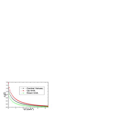
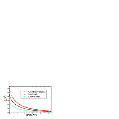
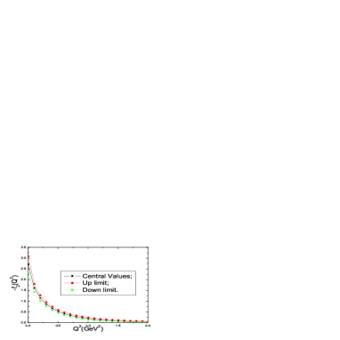
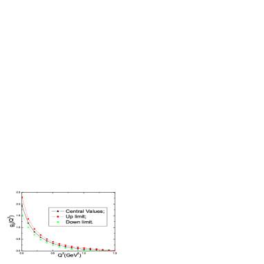
Figure 1: The $f_{1}(Q^{2})$, $g_{1}(Q^{2})$, $f_{2}(Q^{2})$ and $g_{2}(Q^{2})$ with the parameter $Q^{2}$.

The central values of the four form-factors can be approximately fitted into the double-pole formula,

$$F(Q^{2})=\frac{F(0)}{\left(1+\frac{Q^{2}}{m_{A}^{2}}\right)\left(1+\frac{Q^{2}}{m_{B}^{2}}\right)}\,,$$ (15)

here the $F(Q^{2})$ stand for the $f_{1}(Q^{2})$, $f_{2}(Q^{2})$, $g_{1}(Q^{2})$ and $g_{2}(Q^{2})$, the corresponding values of the parameters $m_{A}$ and $m_{B}$ are listed in the Table 1.

$F(Q^{2})$	$m_{A}(GeV)$	$m_{B}(GeV)$
$f_{1}$	$0.95$	$1.55$
$f_{2}$	$0.55$	$0.60$
$g_{1}$	$1.10$	$1.90$
$g_{2}$	$0.43$	$0.75$

Table 1: Numerical values of the parameters $m_{A}$ and $m_{B}$ .

From the numerical values

$$f_{1}(0) = -(1.21\pm 0.34)\,,$$

$$g_{1}(0) = -(0.85\pm 0.34)\,,$$

$$g_{1}(0)/f_{1}(0)_{c} = 0.70\,,$$

$$f_{2}(0) = -(2.70\pm 0.39)\,,$$

$$f_{2}(0)/f_{1}(0)_{c} = 2.23\,,$$

$$g_{2}(0) = 1.92\pm 0.37\,,$$

$$g_{2}(0)/f_{1}(0)_{c} = -1.59\,,$$

$$f_{1}^{\chi}(0) = g_{1}^{\chi}(0)=-1.03\,,$$

$$f_{2}^{\chi}(0) = -g_{2}^{\chi}(0)=-2.31\,,$$

$$f_{1}^{asp}(0) = -1.11\,,$$

$$g_{1}^{asp}(0) = -0.85\,,$$

$$f_{2}^{asp}(0) = -2.67\,,$$

$$g_{2}^{asp}(0) = 1.20\,,$$ (16)

we can see that they are compatible with the experimental data and theoretical estimations (in magnitude), $f_{2}(0)/f_{1}(0)=-1.71\pm 0.12\pm 0.23$ (experimental data) [27]; $g_{1}(0)/f_{1}(0)=-0.340\pm 0.017$ (theoretical estimation)[2]; $f_{1}(0)=-0.988\pm 0.029\pm 0.040$, $g_{1}(0)/f_{1}(0)=-0.287\pm 0.052$, $f_{2}(0)/f_{1}(0)=-1.52\pm 0.81$, $g_{2}(0)/f_{1}(0)=0.63\pm 0.26$ (lattice simulation) [28]. Here the $c$ , $asp$ and $\chi$ stand for the cental values, the asymptotic values and the values in the chiral limit, respectively. The discrepancy may be due to the perturbative $\alpha_{s}$ corrections, additional valence gluons and quark-antiquark pairs. The consistent and complete LCSR analysis should take into account the contributions from the perturbative $\alpha_{s}$ corrections, the distribution amplitudes with additional valence gluons and quark-antiquark pairs, and improve the parameters which enter in the LCSRs.

4 Conclusion

In this work, we calculate the four form-factors $f_{1}(Q^{2})$, $f_{2}(Q^{2})$, $g_{1}(Q^{2})$ and $g_{2}(Q^{2})$ of the $\Sigma\to n$ in the framework of the LCSR approach up to twist-6 three valence quark light-cone distribution amplitudes. The $f_{1}(0)$ is the basic input parameter in extracting the CKM matrix element $|V_{us}|$ from the hyperon decays. The four form-factors $f_{1}(Q^{2})$, $f_{2}(Q^{2})$, $g_{1}(Q^{2})$ and $g_{2}(Q^{2})$ at intermediate and large momentum transfers with $Q^{2}>3GeV^{2}$ have significant contributions from the end-point (soft) terms. The form-factors $f_{1}(Q^{2})$ and $g_{1}(Q^{2})$ are sensitive to the parameter $\lambda_{1}$, small variations of the parameter can lead to large changes of the values, the form-factors $f_{2}(Q^{2})$ and $g_{2}(Q^{2})$ are sensitive to the three parameters $f_{N}$, $\lambda_{1}$ and $f^{d}_{1}$, small variations of those parameters can lead to relatively large changes of the values. The large uncertainties can impair the predictive ability of the sum rules, the parameters $\lambda_{1}$, $f_{N}$ and $f^{d}_{1}$ should be refined to make robust predictions. The numerical values of the four form-factors $f_{1}(0)$, $f_{2}(0)$, $g_{1}(0)$ and $g_{2}(0)$ are compatible with the experimental data and theoretical calculations (in magnitude). The consistent and complete LCSR analysis should take into account the contributions from the perturbative $\alpha_{s}$ corrections, the distribution amplitudes with additional valence gluons and quark-antiquark pairs, and improve the parameters which enter in the LCSRs.

Appendix

$$V_{1}(x_{i},\mu) = 120x_{1}x_{2}x_{3}[\phi_{3}^{0}(\mu)+\phi_{3}^{+}(\mu)(1-3x_{3})],$$

$$V_{2}(x_{i},\mu) = 24x_{1}x_{2}[\phi_{4}^{0}(\mu)+\phi_{3}^{+}(\mu)(1-5x_{3})],$$

$$V_{3}(x_{i},\mu) = 12x_{3}\{\psi_{4}^{0}(\mu)(1-x_{3})+\psi_{4}^{-}(\mu)[x_{1}^{2}+x_{2}^{2}-x_{3}(1-x_{3})]$$

$$+\psi_{4}^{+}(\mu)(1-x_{3}-10x_{1}x_{2})\},$$

$$V_{4}(x_{i},\mu) = 3\{\psi_{5}^{0}(\mu)(1-x_{3})+\psi_{5}^{-}(\mu)[2x_{1}x_{2}-x_{3}(1-x_{3})]$$

$$+\psi_{5}^{+}(\mu)[1-x_{3}-2(x_{1}^{2}+x_{2}^{2})]\},$$

$$V_{5}(x_{i},\mu) = 6x_{3}[\phi_{5}^{0}(\mu)+\phi_{5}^{+}(\mu)(1-2x_{3})],$$

$$V_{6}(x_{i},\mu) = 2[\phi_{6}^{0}(\mu)+\phi_{6}^{+}(\mu)(1-3x_{3})].$$

$$\mathcal{V}_{1}^{u}(x_{3}) = \frac{x_{3}^{2}}{24}(\lambda_{1}C_{\lambda}^{u}+f_{N}C_{f}^{u}),$$

$$C_{\lambda}^{u} = -(1-x_{3})[11+131\,x_{3}-169x_{3}^{2}+63x_{3}^{3}-30\,f_{1}^{d}\,(3+11x_{3}-17x_{3}^{2}+7x_{3}^{3})]$$

$$-12\,(3-10\,f_{1}^{d})\,\ln x_{3},$$

$$C_{f}^{u} = -(1-x_{3})\,[1441+505x_{3}-3371x_{3}^{2}+3405x_{3}^{3}-1104x_{3}^{4}-24V_{1}^{d}$$

$$(207-3x_{3}-368x_{3}^{2}+412x_{3}^{3}-138x_{3}^{4})]-12(73-220\,V_{1}^{d})\,\ln x_{3},$$

$$\phi_{3}^{0}=\phi_{6}^{0}=f_{N}\,,\hskip 8.5359pt \phi_{4}^{0}=\phi_{5}^{0}=\frac{1}{2}\left(\lambda_{1}+f_{N}\right)\,,$$

$$\xi_{4}^{0}=\xi_{5}^{0}=\frac{1}{6}\lambda_{2}\,, \psi_{4}^{0}=\psi_{5}^{0}=\frac{1}{2}\left(f_{N}-\lambda_{1}\right)\,.$$

$$\tilde{\phi}_{3}^{-} = \frac{21}{2}A_{1}^{u},$$

$$\tilde{\phi}_{3}^{+} = \frac{7}{2}(1-3V_{1}^{d}),$$

$$\phi_{4}^{-} = \frac{5}{4}\left(\lambda_{1}(1-2f_{1}^{d}-4f_{1}^{u})+f_{N}(2A_{1}^{u}-1)\right)\,,$$

$$\phi_{4}^{+} = \frac{1}{4}\left(\lambda_{1}(3-10f_{1}^{d})-f_{N}(10V_{1}^{d}-3)\right)\,,$$

$$\psi_{4}^{-} = -\frac{5}{4}\left(\lambda_{1}(2-7f_{1}^{d}+f_{1}^{u})+f_{N}(A_{1}^{u}+3V_{1}^{d}-2)\right)\,,$$

$$\psi_{4}^{+} = -\frac{1}{4}\left(\lambda_{1}(-2+5f_{1}^{d}+5f_{1}^{u})+f_{N}(2+5A_{1}^{u}-5V_{1}^{d})\right)\,,$$

$$\xi_{4}^{-} = \frac{5}{16}\lambda_{2}(4-15f_{2}^{d})\,,$$

$$\xi_{4}^{+} = \frac{1}{16}\lambda_{2}(4-15f_{2}^{d})\,,$$

$$\phi_{5}^{-} = \frac{5}{3}\left(\lambda_{1}(f_{1}^{d}-f_{1}^{u})+f_{N}(2A_{1}^{u}-1)\right)\,,$$

$$\phi_{5}^{+} = -\frac{5}{6}\left(\lambda_{1}(4f_{1}^{d}-1)+f_{N}(3+4V_{1}^{d})\right)\,,$$

$$\psi_{5}^{-} = \frac{5}{3}\left(\lambda_{1}(f_{1}^{d}-f_{1}^{u})+f_{N}(2-A_{1}^{u}-3V_{1}^{d})\right)\,,$$

$$\psi_{5}^{+} = -\frac{5}{6}\left(\lambda_{1}(-1+2f_{1}^{d}+2f_{1}^{u})+f_{N}(5+2A_{1}^{u}-2V_{1}^{d})\right)\,,$$

$$\xi_{5}^{-} = -\frac{5}{4}\lambda_{2}f_{2}^{d}\,,$$

$$\xi_{5}^{+} = \frac{5}{36}\lambda_{2}(2-9f_{2}^{d})\,,$$

$$\phi_{6}^{-} = \phantom{-}\frac{1}{2}\left(\lambda_{1}(1-4f_{1}^{d}-2f_{1}^{u})+f_{N}(1+4A_{1}^{u})\right)\,,$$

$$\phi_{6}^{+} = -\frac{1}{2}\left(\lambda_{1}(1-2f_{1}^{d})+f_{N}(4V_{1}^{d}-1)\right)\,.$$

References

[1] E. Blucher, et al, hep-ph/0512039; and references
therein.
[2] N. Cabibbo, E. C. Swallow , R. Winston, Phys. Rev. Lett. 92 (2004)
251803; N. Cabibbo, E. C. Swallow, R. Winston, Ann. Rev. Nucl. Part.
Sci. 53 (2003) 39.
[3] M. Ademollo and R. Gatto, Phys. Rev. Lett. 13 (1964) 264 .
[4]
J. F. Donoghue, B. R. Holstein and S. W. Klimt, Phys. Rev. D
35 (1987) 934; F. Schlumpf,
Phys. Rev. D51 (1995) 2262.
[5]
R. Flores-Mendieta, E. Jenkins and A. V. Manohar, Phys. Rev. D58 (1998) 094028; R. Flores-Mendieta, Phys. Rev. D70,
(2004) 114036.
[6] A. Krause, Helv. Phys. Acta 63 (1990) 3;
J. Anderson and M. A. Luty, Phys. Rev. D47 (1993) 4975;
N. Kaiser, Phys. Rev. C64 (2001) 028201; G. Villadoro
Phys. Rev. D74 (2006) 014018.
[7] Z. G. Wang, S. L. Wan, hep-ph/0608164.
[8]
I. I. Balitsky, V. M. Braun and A. V. Kolesnichenko, Nucl. Phys.
B312 (1989) 509; V. L. Chernyak and I. R. Zhitnitsky, Nucl.
Phys. B345 (1990) 137; V. L. Chernyak and A. R. Zhitnitsky,
Phys. Rept. 112 (1984) 173.
[9]
V. M. Braun, hep-ph/9801222; P. Colangelo and A. Khodjamirian,
hep-ph/0010175.
[10] M. A. Shifman, A. I. Vainshtein and V. I. Zakharov,
Nucl. Phys. B147 (1979) 385, 448.
[11]
V. Braun, R. J. Fries, N. Mahnke and E. Stein, Nucl. Phys. B
589 (2000) 381; Erratum-ibid. B607 (2001) 433.
[12] V. M. Braun, A. Lenz, N. Mahnke,
Phys. Rev. D65 (2002) 074011;
A. Lenz, M. Wittmann, E. Stein, Phys. Lett. B581 (2004) 199;
V. M. Braun, A. Lenz, G. Peters, A.V. Radyushkin, Phys. Rev. D73 (2005)
034020.
[13] Z. G. Wang, S. L. Wan, W. M. Yang,
Phys. Rev. D73 (2006) 094011; Z. G. Wang, S. L. Wan, W. M. Yang, Eur. Phys. J. C47 (2006)
375.
[14] V. M. Braun, A. Lenz, M. Wittmann, Phys. Rev. D73 (2006)
094019.
[15] M. Q. Huang, D. W. Wang, Phys. Rev. D69 (2004)
094003; M. Q. Huang, D. W. Wang, hep-ph/0608170.
[16]
B. L. Ioffe, Nucl. Phys. B188 (1981) 317; B. L. Ioffe, A. V.
Smilga , Nucl. Phys. B232 (1984) 109.
[17] V. Chung, H. G. Dosch, M. Kremer, D. Scholl,
Nucl. Phys.B197 (1982) 55; H. G. Dosch, M. Jamin and S.
Narison, Phys. Lett.B220 (1989) 251.
[18]
V. L. Chernyak and I. R. Zhitnitsky, Nucl. Phys. B246 (1984)
52; I. D. King and C. T. Sachrajda, Nucl. Phys. B279 (1987)
785; V. L. Chernyak, A. A. Ogloblin and I. R. Zhitnitsky, Sov. J.
Nucl. Phys. 48 (1988) 536; Z. Phys. C 42 (1989) 583.
[19]
I. I. Balitsky and V. M. Braun, Nucl. Phys. B311 (1989) 541.
[20]
M. Diehl, T. Feldmann, R. Jakob and P. Kroll, Eur. Phys. J. C8 (1999) 409.
[21]
G. P. Lepage and S. J. Brodsky, Phys. Rev. Lett. 43 (1979) 545,
1625 (E); V. A. Avdeenko, V. L. Chernyak and S. A. Korenblit,
Yad. Fiz. 33 (1981) 481;
S. J. Brodsky, G. P. Lepage and A. A. Zaidi,
Phys. Rev. D23 (1981) 1152; S. J. Brodsky and G. P. Lepage,
A. I. Milshtein and V. S. Fadin, Yad. Fiz. 35 (1982) 1603.
[22] C. B. Chiu, J. Pasupathy, S. L. Wilson, Phys. Rev. D32 (1985) 1786; W. Y. Hwang, K. C. Yang ,
Phys. Rev. D49 (1994) 460.
[23] S. J. Brodsky, G. P. Lepage, Phys. Rev. D24 (1981)
1808.
[24] J. Gronberg, et al, Phys. Rev. D57 (1998) 33;
and references therein.
[25] S. Weinberg, Phys. Rev. 112 (1958) 1375.
[26] T. Huang, Z. H. Li, X. Y. Wu, Phys. Rev. D63 (2001) 094001; Z. G. Wang, M. Z. Zhou, T.
Huang, Phys. Rev. D67 (2003) 094006.
[27] S. Y. Hsueh et al, Phys. Rev. D38 (1988)
2056.
[28] D. Guadagnoli, V. Lubicz, M. Papinutto, S. Simula,
hep-ph/0606181.