THEORETICAL OVERVIEW ON TAU PHYSICS

Abstract

Precise measurements of the $\tau$ lepton properties provide stringent tests of the Standard Model structure and accurate determinations of its parameters. We overview the present status of a few selected topics: lepton universality, QCD tests and the determination of $\alpha_{s}$, $m_{s}$ and $|V_{us}|$ from hadronic $\tau$ decays, and lepton flavor violation phenomena.

1 Lepton Universality

In the Standard Model all lepton doublets have identical couplings to the $W$ boson. Comparing the measured decay widths of leptonic or semileptonic decays which only differ by the lepton flavor, one can test experimentally that the $W$ interaction is indeed the same, i.e. that  $g_{e}=g_{\mu}=g_{\tau}\equiv g\,$. As shown in Table 1, the present data verify the universality of the leptonic charged-current couplings to the 0.2% level.[1][3]

Present constraints on $|g_{l}/g_{l^{\prime}}|$. $B_{\tau\to\mu}/B_{\tau\to e}$ $B_{W\to\mu}/B_{W\to e}$ $B_{\pi\to\mu}/B_{\pi\to e}$ $|g_{\mu}/g_{e}|$ $1.0000\pm 0.0020$ $0.997\pm 0.010$ $1.0017\pm 0.0015$ $B_{\tau\to e}\,\tau_{\mu}/\tau_{\tau}$ $B_{W\to\tau}/B_{W\to\mu}$ $\Gamma_{\tau\to\pi}/\Gamma_{\pi\to\mu}$ $\Gamma_{\tau\to K}/\Gamma_{K\to\mu}$ $|g_{\tau}/g_{\mu}|$ $1.0004\pm 0.0022$ $1.039\pm 0.013$ $0.996\pm 0.005$ $0.979\pm 0.017$ $B_{\tau\to\mu}\,\tau_{\mu}/\tau_{\tau}$ $B_{W\to\tau}/B_{W\to e}$ $|g_{\tau}/g_{e}|$ $1.0004\pm 0.0023$ $1.036\pm 0.014$

The $\tau$ leptonic branching fractions and the $\tau$ lifetime are already known with a precision of $0.3\%$. It remains to be seen whether BABAR and BELLE could make further improvements. The $\mu$ lifetime has been measured to a much better precision of $10^{-5}$. The universality tests require also a good determination of $m_{\tau}^{5}$, which is only known to the $0.08\%$ level. An improved measurement of the $\tau$ mass could be expected from BES-III, through a detailed analysis of $\sigma(e^{+}e^{-}\to\tau^{+}\tau^{-})$ at threshold.[4][6]

2 Hadronic Tau Decays

The semileptonic decay modes $\tau^{-}\to\nu_{\tau}H^{-}$ probe the matrix element of the left–handed charged current between the vacuum and the final hadronic state $H^{-}$.

For the decay modes with lowest multiplicity, $\tau^{-}\to\nu_{\tau}\pi^{-}$ and $\tau^{-}\to\nu_{\tau}K^{-}$, the relevant matrix elements are already known from the measured decays $\pi^{-}\to\mu^{-}\bar{\nu}_{\mu}$ and $K^{-}\to\mu^{-}\bar{\nu}_{\mu}$. The corresponding $\tau$ decay widths can then be accurately predicted. As shown in Table 1, the predictions are in good agreement with the measured values. Assuming universality, these decay modes determine the ratio[2, 7]

$$\frac{|V_{us}|\,f_{K}}{|V_{ud}|\,f_{\pi}}\,=\,\left\{\begin{array}[]{cc}0.27618\pm 0.00048&\qquad[\,\Gamma(K^{-}\to\mu^{-}\bar{\nu}_{\mu})/\Gamma(\pi^{-}\to\mu^{-}\bar{\nu}_{\mu})\,]\\ 0.267\pm 0.005&\qquad[\,\Gamma(\tau^{-}\to\nu_{\tau}K^{-})/\Gamma(\tau^{-}\to\nu_{\tau}\pi^{-})\,]\end{array}\right..$$ (1)

The very different accuracy of these two numbers reflects the present poor precision on $\Gamma(\tau^{-}\to\nu_{\tau}K^{-})$.

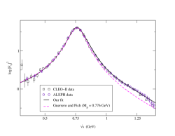
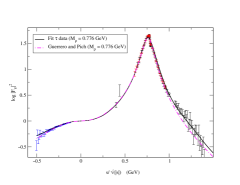
Figure 1: Pion form factor from $\tau$ data[18, 19] (left) and $e^{+}e^{-}$ data[20, 21] (right), compared with theoretical predictions.[8, 10] The dashed lines correspond to the result in Eq. (3).

For the two–pion final state, the hadronic matrix element is parameterized in terms of the so-called pion form factor  [$s\equiv(p_{\pi^{-}}\!+p_{\pi^{0}})^{2}$]:

$$\langle\pi^{-}\pi^{0}|\bar{d}\gamma^{\mu}u|0\rangle\equiv\sqrt{2}\,F_{\pi}(s)\,\left(p_{\pi^{-}}-p_{\pi^{0}}\right)^{\mu}\,.$$ (2)

A dynamical understanding of the pion form factor can be achieved,[8][12] by using analyticity, unitarity and some general properties of QCD, such as chiral symmetry[13][15] and the short-distance asymptotic behavior.[16, 17] Putting all these fundamental ingredients together, one gets the result[8]

$$F_{\pi}(s)={M_{\rho}^{2}\over M_{\rho}^{2}-s-iM_{\rho}\Gamma_{\rho}(s)}\;\exp{\left\{-{s\,\mbox{\rm Re}\left[A(s)\right]\over 96\pi^{2}f_{\pi}^{2}}\right\}},$$ (3)

where

$$A(s)\equiv\log{\left({m_{\pi}^{2}\over M_{\rho}^{2}}\right)}+8{m_{\pi}^{2}\over s}-{5\over 3}+\sigma_{\pi}^{3}\log{\left({\sigma_{\pi}+1\over\sigma_{\pi}-1}\right)}\,,\qquad\sigma_{\pi}\equiv\sqrt{1-4m_{\pi}^{2}/s}$$ (4)

contains the one-loop chiral logarithms and the off-shell $\rho$ width is given by[8, 9]

$$\Gamma_{\rho}(s)\,=\,\theta(s-4m_{\pi}^{2})\,\sigma_{\pi}^{3}\,M_{\rho}\,s/(96\pi f_{\pi}^{2})\,.$$ (5)

This prediction, which only depends on $M_{\rho}$, $m_{\pi}$ and the pion decay constant $f_{\pi}$, is compared with the data in Fig. 1.[10] The agreement is rather impressive and extends to negative $s$ values, where the $e^{-}\pi$ elastic data sits. The small effect of heavier $\rho$ resonance contributions and additional higher-order (in the Chiral Perturbation Theory and $1/N_{C}$ expansions[17]) corrections can be easily included, at the price of having some free parameters which decrease the predictive power.[10][12] This gives a better description of the $\rho^{\prime}$ shoulder around 1.2 GeV (continuous lines in Fig. 1).

More recently, the decay $\tau\to\nu_{\tau}K\pi$ has been studied in Ref. JPP:06. The hadronic spectrum is characterized by two form factors,

$$\frac{d\Gamma_{K\pi}}{d\sqrt{s}}=\frac{G_{F}^{2}|V_{us}|^{2}m_{\tau}^{3}}{32\pi^{3}s}\biggl{(}1-\frac{s}{m_{\tau}^{2}}\biggr{)}^{\!2}\Biggl{[}\biggl{(}1+2\,\frac{s}{m_{\tau}^{2}}\biggr{)}q_{K\pi}^{3}|F_{+}^{K\pi}(s)|^{2}+\frac{3\Delta_{K\pi}^{2}}{4s}\,q_{K\pi}^{\phantom{3}}|F_{0}^{K\pi}(s)|^{2}\Biggr{]}$$ (6)

where $q_{K\pi}^{\phantom{3}}=\frac{1}{2\sqrt{s}}\,\lambda^{1/2}(s,m_{K}^{2},m_{\pi}^{2})$ and $\Delta_{K\pi}=m_{K}^{2}-m_{\pi}^{2}$. The vector form factor $F_{+}^{K\pi}(s)$ has been described in an analogous way to $F_{\pi}(s)$, while the scalar component $F_{0}^{K\pi}(s)$ takes also into account additional information from $K\pi$ scattering data through dispersion relations.[7, 23] The decay width is dominated by the $K^{*}(892)$ contribution, with a predicted branching ratio Br$[\tau\to\nu_{\tau}K^{*}]=(1.253\pm 0.078)\%$, while the scalar component is found to be Br$[\tau\to\nu_{\tau}(K\pi)_{\rm S-wave}]=(3.88\pm 0.19)\cdot 10^{-4}$.

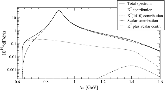
Figure 2: Differential $\tau\to\nu_{\tau}K\pi$ decay distribution, together with the individual contributions from the $K^{*}(892)$ and $K^{*}(1410)$ vector mesons as well as the scalar component residing in $F_{0}^{K\pi}(s)$.[22]

The dynamical structure of other hadronic final states can be investigated in a similar way. The $\tau\to\nu_{\tau}3\pi$ decay mode was studied in Ref. DPP:01, where a theoretical description of the measured structure functions[25][27] was provided. A detailed analysis of other $\tau$ decay modes into three final pseudoscalar mesons is in progress.[28] The more involved $\tau\to\nu_{\tau}4\pi$ and $e^{+}e^{-}\to 4\pi$ transitions have been also studied.[29]

3 The Hadronic Tau Decay Width: $\mathrm{\alpha_{s}}$

The inclusive character of the total $\tau$ hadronic width renders possible an accurate calculation of the ratio[30][34]

$$R_{\tau}\equiv{\Gamma[\tau^{-}\rightarrow\nu_{\tau}\,\mbox{\rm hadrons}\,(\gamma)]\over\Gamma[\tau^{-}\rightarrow\nu_{\tau}e^{-}{\bar{\nu}}_{e}(\gamma)]}\,=\,R_{\tau,V}+R_{\tau,A}+R_{\tau,S}\,,$$ (7)

using analyticity constraints and the Operator Product Expansion. One can separately compute the contributions associated with specific quark currents. $R_{\tau,V}$ and $R_{\tau,A}$ correspond to the Cabibbo–allowed decays through the vector and axial-vector currents, while $R_{\tau,S}$ contains the remaining Cabibbo–suppressed contributions.

The theoretical prediction for $R_{\tau,V+A}$ can be expressed as[32]

$$R_{\tau,V+A}=3\,|V_{ud}|^{2}\,S_{\mathrm{EW}}\left\{1+\delta_{\mathrm{EW}}^{\prime}+\delta_{\mathrm{P}}+\delta_{\mathrm{NP}}\right\}.$$ (8)

The factors $S_{\mathrm{EW}}=1.0194$ and $\delta_{\mathrm{EW}}^{\prime}=0.0010$ contain the electroweak corrections at the leading[35] and next-to-leading[36] logarithm approximation. The dominant correction ($\sim 20\%$) is the purely perturbative contribution $\delta_{\mathrm{P}}$, which is fully known[32] to $O(\alpha_{s}^{3})$ and includes a resummation of the most important higher-order corrections.[33]

Non-perturbative contributions are suppressed by six powers of the $\tau$ mass and, therefore, are very small.[32] Their numerical size has been determined from the invariant–mass distribution of the final hadrons in $\tau$ decay, through the study of weighted integrals,[37]

$$R_{\tau}^{kl}\equiv\int_{0}^{m_{\tau}^{2}}ds\,\left(1-{s\over m_{\tau}^{2}}\right)^{k}\,\left({s\over m_{\tau}^{2}}\right)^{l}\,{dR_{\tau}\over ds}\,,$$ (9)

which can be calculated theoretically in the same way as $R_{\tau}$. The predicted suppression[32] of the non-perturbative corrections has been confirmed by ALEPH,[27] CLEO[38] and OPAL.[39] The most recent analysis gives[27]

$$\delta_{\mathrm{NP}}\,=\,-0.004\pm 0.002\,.$$ (10)

The QCD prediction for $R_{\tau,V+A}$ is then completely dominated by the perturbative contribution; non-perturbative effects being smaller than the perturbative uncertainties from uncalculated higher-order corrections. The result turns out to be very sensitive to the value of $\alpha_{s}(m_{\tau})$, allowing for an accurate determination of the fundamental QCD coupling.[31, 32] The experimental measurement $R_{\tau,V+A}=3.471\pm 0.011$ implies[40]

$$\alpha_{s}(m_{\tau})=0.345\pm 0.004_{\mathrm{exp}}\pm 0.009_{\mathrm{th}}\,.$$ (11)

The strong coupling measured at the $\tau$ mass scale is significantly larger than the values obtained at higher energies. From the hadronic decays of the $Z$, one gets $\alpha_{s}(M_{Z})=0.1186\pm 0.0027$,[3] which differs from the $\tau$ decay measurement by more than twenty standard deviations. After evolution up to the scale $M_{Z}$,[41] the strong coupling constant in (11) decreases to[40]

$$\alpha_{s}(M_{Z})=0.1215\pm 0.0012\,,$$ (12)

in agreement with the direct measurements at the $Z$ peak and with a similar accuracy. The comparison of these two determinations of $\alpha_{s}$ in two extreme energy regimes, $m_{\tau}$ and $M_{Z}$, provides a beautiful test of the predicted running of the QCD coupling; i.e. a very significant experimental verification of asymptotic freedom.

4 Cabibbo–Suppressed Tau Decays: $\mathbf{V_{\!us}}$ and $\mathbf{m_{s}}$

The separate measurement of the $|\Delta S|=0$ and $|\Delta S|=1$  $\tau$ decay widths allows us to pin down the SU(3) breaking effect induced by the strange quark mass,[42][49] through the differences:[43]

$$\delta R_{\tau}^{kl}\equiv{R_{\tau,V+A}^{kl}\over|V_{ud}|^{2}}-{R_{\tau,S}^{kl}\over|V_{us}|^{2}}\,\approx\,24\,{m_{s}^{2}(m_{\tau})\over m_{\tau}^{2}}\,\Delta_{kl}(\alpha_{s})-48\pi^{2}\,{\delta O_{4}\over m_{\tau}^{4}}\,Q_{kl}(\alpha_{s})\,.$$ (13)

The perturbative QCD corrections $\Delta_{kl}(\alpha_{s})$ and $Q_{kl}(\alpha_{s})$ are known to $O(\alpha_{s}^{3})$ and $O(\alpha_{s}^{2})$, respectively.[43, 49] Since the longitudinal contribution to $\Delta_{kl}(\alpha_{s})$ does not converge well, the $J=0$ QCD expression is replaced by its corresponding phenomenological hadronic parametrization,[48] which is much more precise because it is dominated by far by the well-known kaon pole. The small non-perturbative contribution, $\delta O_{4}\equiv\langle 0|m_{s}\bar{s}s-m_{d}\bar{d}d|0\rangle=-(1.5\pm 0.4)\times 10^{-3}\;\mbox{\rm GeV}^{4}$, has been estimated with Chiral Perturbation Theory techniques.[43]

From the measured moments $\delta R_{\tau}^{k0}$ ($k=0,1,2,3,4$),[50, 51] it is possible to determine the strange quark mass; however, the extracted value depends sensitively on the modulus of the Cabibbo–Kobayashi–Maskawa matrix element $|V_{us}|$. It appears then natural to turn things around and, with an input for $m_{s}$ obtained from other sources, to actually determine $|V_{us}|$.[48] The most sensitive moment is $\delta R_{\tau}^{00}$:

$$|V_{us}|^{2}=\frac{R^{(0,0)}_{\tau,S}}{\frac{R^{(0,0)}_{\tau,V+A}}{|V_{ud}|^{2}}-\delta R^{(0,0)}_{\tau,{\mathrm{th}}}}\,.$$ (14)

Using $m_{s}(2~{}\mathrm{GeV})=(95\pm 20)~{}\mathrm{MeV}$, which includes the most recent determinations of $m_{s}$ from lattice and QCD Sum Rules,[7] one obtains $\delta R^{00}_{\tau,{\mathrm{th}}}=0.218\pm 0.026$.[48] This prediction is much smaller than $R^{(0,0)}_{\tau,V+A}/|V_{ud}|^{2}$, making the theoretical uncertainty in (14) negligible in comparison with the experimental input $R^{(0,0)}_{\tau,V+A}=3.469\pm 0.014$ and $R^{(0,0)}_{\tau,S}=0.1677\pm 0.0050$.[51] Taking $|V_{ud}|=0.9738\pm 0.0005$,[2] one finally gets[48]

$$|V_{us}|=0.2208\pm 0.0033_{\mathrm{exp}}\pm 0.0009_{\mathrm{th}}=0.2208\pm 0.0034\,.$$ (15)

This result is competitive with the standard determination from $K_{e3}$ decays, $|V_{us}|=0.2236\pm 0.0029$.[7] The precision is expected to be highly improved in the near future due to the fact that the error is dominated by the experimental uncertainty, which can be reduced with the better BABAR and BELLE data samples. Therefore, the $\tau$ data has the potential to provide the best determination of $|V_{us}|$.

One can further use the value of $|V_{us}|$ thus obtained in (15) and determine the strange quark mass from higher $\delta R_{\tau}^{k0}$ moments with $k\not=0$. One finds in this way $m_{s}(m_{\tau})=(84\pm 23)$ MeV, which implies $m_{s}(2~{}\mathrm{GeV})=(81\pm 22)$ MeV. With future high-precision $\tau$ data, a simultaneous fit of $m_{s}$ and $|V_{us}|$ should become possible.

5 New Physics

Convincing evidence of neutrino oscillations has been obtained recently, showing that $\nu_{e}\to\nu_{\mu,\tau}$ and $\nu_{\mu}\to\nu_{\tau}$ lepton-flavor-violating transitions do occur.[52][55] The non-zero values of neutrino masses constitute a clear indication of new physics beyond the Standard Model framework. The simplest possibility would be the existence of right-handed neutrino components. However, those singlet $\nu_{iR}$ fields would not have any Standard Model interaction (sterile neutrinos). Moreover, the Standard Model gauge symmetry would allow for a right-handed Majorana neutrino mass term of arbitrary size, not related to the ordinary Higgs mechanism.

In the absence of right-handed neutrino fields, it is still possible to have non-zero Majorana neutrino masses, generated through the unique $SU(3)_{C}\otimes SU(2)_{L}\otimes U(1)_{Y}$ invariant operator with dimension five:[56]

$$\Delta{\cal L}\;=\;-{c_{ij}\over\Lambda}\;\bar{L}_{i}\,\tilde{\phi}\,\tilde{\phi}^{t}\,L_{j}^{c}\;+\;\mathrm{h.c.}\stackrel{{\scriptstyle SSB}}{{\quad\;\longrightarrow\quad\;}}{\cal L}_{M}=-{1\over 2}\,\bar{\nu}_{iL}M_{ij}\,\nu_{jL}^{c}+\mathrm{h.c.}\,,$$ (16)

where $\phi$ and $L_{i}$ are the scalar and $i$-flavored lepton $SU(2)_{L}$ doublets, $\tilde{\phi}\equiv i\,\tau_{2}\,\phi^{*}$ and $L_{i}^{c}\equiv\mathcal{C}\bar{L}_{i}^{t}$. After spontaneous symmetry breaking, $<\phi^{(0)}>=v/\sqrt{2}$, this operator generates a Majorana mass term for the left-handed neutrinos with $M_{ij}=c_{ij}v^{2}/\Lambda$. The Majorana mass matrix mixes neutrinos and anti-neutrinos, violating lepton number by two units. Clearly, new physics is called for. Taking $m_{\nu}\stackrel{{\scriptstyle>}}{{{}_{\sim}}}0.05$ eV, as suggested by atmospheric neutrino data, one gets $\Lambda/c_{ij}\stackrel{{\scriptstyle<}}{{{}_{\sim}}}10^{15}$ GeV, amazingly close to the expected scale of Gran Unification.

With non-zero neutrino masses, the leptonic charged current interactions, involve a flavor mixing matrix $V_{L}$. Neglecting possible CP-violating phases, the present data on neutrino oscillations implies the mixing structure

$$V_{L}\;\sim\;\left[\begin{array}[]{ccc}{1\over\sqrt{2}}\,(1+\lambda)&{1\over\sqrt{2}}\,(1-\lambda)&\epsilon\\ -{1\over 2}\,(1-\lambda+\epsilon)&{1\over 2}\,(1+\lambda-\epsilon)&{1\over\sqrt{2}}\\ {1\over 2}\,(1-\lambda-\epsilon)&-{1\over 2}\,(1+\lambda+\epsilon)&{1\over\sqrt{2}}\end{array}\right],$$ (17)

with $\lambda\sim 0.2$ and $\epsilon<0.2$. Therefore, the mixing among leptons appears to be very different from the one in the quark sector. The number of relevant phases characterizing the matrix $V_{L}$ depends on the Dirac or Majorana nature of neutrinos. With only three Majorana (Dirac) neutrinos, the $3\times 3$ matrix $V_{L}$ involves six (four) independent parameters: three mixing angles and three (one) phases.

At present, we still ignore whether neutrinos are Dirac or Majorana fermions. Another important question to be addressed in the future concerns the possibility of leptonic CP violation and its relevance for explaining the baryon asymmetry of our universe through a leptogenesis mechanism.

The existence of lepton flavor violation opens a very interesting window to improve our understanding of flavor dynamics. The smallness of the neutrino masses implies a strong suppression of neutrinoless lepton-flavor-violation processes. However, this suppression can be avoided in models with other sources of lepton flavor violation, not related to $m_{\nu_{i}}$. The present experimental limits on lepton-flavor-violating $\tau$ decays, at the $10^{-7}$ level,[57, 58] are already sensitive to new-physics scales of the order of a few TeV. Further improvements at future experiments would allow to explore interesting and totally unknown phenomena.

References

- [1] A. Pich, Nucl. Phys. (Proc. Suppl.) 123, 1 (2003).
- [2] W.-M. Yao et al., The Review of Particle Physics, Journal of Physics G 33, 1 (2006).
- [3] The LEP Collaborations ALEPH, DELPHI, L3, OPAL and the LEP Electroweak Working Group, arXiv:hep-ph/0511027; http://www.cern.ch/LEPEWWG.
- [4] P. Ruiz-Femenía and A. Pich, Phys. Rev. D64, 053001 (2001).
- [5] M.B. Voloshin, Phys. Lett. B 556, 153 (2003).
- [6] B.H. Smith and M.B. Voloshin, Phys. Lett. B 324, 117 (1994); 333, 564 (1994).
- [7] M. Jamin, J.A. Oller and A. Pich, arXiv:hep-ph/0605095.
- [8] F. Guerrero and A. Pich, Phys. Lett. B 412, 382 (1997).
- [9] D. Gómez–Dumm, A. Pich and J. Portolés, Phys. Rev. D 62, 054014 (2000).
- [10] A. Pich and J. Portolés, Phys. Rev. D63, 093005 (2001); Nucl. Phys. B (Proc. Suppl.) 121, 179 (2003).
- [11] J.J. Sanz-Cillero and A. Pich, Eur. Phys. J. C 27, 587 (2003).
- [12] I. Rosell, J.J. Sanz-Cillero and A. Pich, JHEP 0408, 042 (2004).
- [13] J. Gasser and H. Leutwyler, Nucl. Phys. B 250, 465, 517, 539 (1985).
- [14] G. Ecker, Prog. Part. Nucl. Phys. 35, 1 (1995).
- [15] A. Pich, Rep. Prog. Phys. 58, 563 (1995); arXiv:hep-ph/9802419.
- [16] G. Ecker et al., Nucl. Phys. B 321, 311 (1989); Phys. Lett. B 233, 425 (1989).
- [17] A. Pich, Colourless Mesons in a Polychromatic World, arXiv:hep-ph/0205030.
- [18] ALEPH Collab., Z. Phys. C 76, 15 (1997).
- [19] CLEO Collab., Phys. Rev. D61, 112002 (2000).
- [20] L.M. Barkov et al., Nucl. Phys. B 256, 365 (1985).
- [21] S.R. Amendolia et al., Nucl. Phys. B 277, 168 (1986).
- [22] M. Jamin, A. Pich and J. Portolés, Phys. Lett. B 640, 176 (2006).
- [23] M. Jamin, J.A. Oller and A. Pich, Nucl. Phys. B 622, 279 (2002); 587, 331 (2000).
- [24] D. Gómez–Dumm, A. Pich and J. Portolés, Phys. Rev. D69, 073002 (2004).
- [25] CLEO Collab., Phys. Rev. D61, 052004, 012002 (2000).
- [26] OPAL Collab., Z. Phys. C 75, 593 (1997).
- [27] ALEPH Collab., Phys. Rep. 421, 191 (2005); Eur. Phys. J. C 4, 409 (1998); Phys. Lett. B 307, 209 (1993).
- [28] P. Roig and J. Portolés, work in progress.
- [29] G. Ecker and R. Unterdorfer, Eur. Phys. J. C 24, 535 (2002).
- [30] E. Braaten, Phys. Rev. Lett. 60, 1606 (1988); Phys. Rev. D39, 1458 (1989).
- [31] S. Narison and A. Pich, Phys. Lett. B 211, 183 (1988).
- [32] E. Braaten, S. Narison and A. Pich, Nucl. Phys. B 373, 581 (1992).
- [33] F. Le Diberder and A. Pich, Phys. Lett. B 286, 147 (1992).
- [34] A. Pich, Nucl. Phys. B (Proc. Suppl.) 39B,C, 326 (1995).
- [35] W.J. Marciano and A. Sirlin, Phys. Rev. Lett. 61, 1815 (1988).
- [36] E. Braaten and C.S. Li, Phys. Rev. D 42, 3888 (1990).
- [37] F. Le Diberder and A. Pich, Phys. Lett. B 289, 165 (1992).
- [38] CLEO Collab., Phys. Lett. B 356, 580 (1995).
- [39] OPAL Collab., Eur. Phys. J. C 7, 571 (1999).
- [40] M. Davier, A. Höcker and Z. Zhang, arXiv:hep-ph/0507078.
- [41] G. Rodrigo, A. Pich and A. Santamaria, Phys. Lett. B 424, 367 (1998).
- [42] M. Davier, Nucl. Phys. B (Proc. Suppl.) 55C, 395 (1997). S. Chen, Nucl. Phys. B (Proc. Suppl.) 64, 265 (1998). S. Chen, M. Davier and A. Höcker, Nucl. Phys. B (Proc. Suppl.) 76, 369 (1999).
- [43] A. Pich and J. Prades, JHEP 9910, 004 (1999); 9806, 013 (1998); Nucl. Phys. B (Proc. Suppl.) 86, 236 (2000); 74, 309 (1999). J. Prades, Nucl. Phys. B (Proc. Suppl.) 76, 341 (1999).
- [44] S. Chen et al., Eur. Phys. J. C 22, 31 (2001). M. Davier et al., Nucl. Phys. B (Proc. Suppl.) 98, 319 (2001).
- [45] K.G. Chetyrkin, J.H. Kühn and A.A. Pivovarov, Nucl. Phys. B 533, 473 (1998).
- [46] J.G. Körner F. Krajewski and A.A. Pivovarov, Eur. Phys. J. C 20, 259 (2001).
- [47] J. Kambor and K. Maltman, Phys. Rev. D62, 093023 (2000); Nucl. Phys. A 680, 155 (2000); Nucl. Phys. B (Proc. Suppl.) 98, 314 (2001).
- [48] E. Gámiz et al., Phys. Rev. Lett.94, 011803 (2005); JHEP 0301, 060 (2003).
- [49] P. A. Baikov, K. G. Chetyrkin and J. H. Kühn, Phys. Rev. Lett.95, 012003 (2005).
- [50] ALEPH Collab., Eur. Phys. J. C 11, 599 (1999); 10, 1 (1999).
- [51] OPAL Collab., Eur. Phys. J. C 35, 437 (2004).
- [52] SNO Collab., Phys. Rev. C72, 055502 (2005); Phys. Rev. Lett.92, 181301 (2004); 89, 011301, 011302 (2002); 87, 071301 (2001).
- [53] Super-Kamiokande Collab., arXiv:hep-ex/0607059; Phys. Rev. D73, 112001 (2006); 71, 112005 (2005); Phys. Rev. Lett.93, 101801 (2004); 86, 5656, 5651 (2001); 85, 3999 (2000); 82, 2644 (1999); 81, 1562 (1998); Phys. Lett. B 539, 179 (2002).
- [54] KamLAND Collab., Phys. Rev. Lett.94, 081801 (2005); 90, 021802 (2003).
- [55] K2K Collab., arXiv:hep-ex/0606032; Phys. Rev. Lett.94, 081802 (2005); 90, 041801 (2003).
- [56] S. Weinberg, Phys. Rev. Lett.43, 1566 (1979).
- [57] BABAR Collab., Phys. Rev. Lett.96, 041801 (2006); 95, 041802, 191801 (2005); 92, 121801 (2004).
- [58] BELLE Collab., Phys. Lett. B 640, 138 (2006); 639, 159 (2006); 632, 51 (2006); 622, 218 (2005); 589, 103 (2004); Phys. Rev. Lett.93, 081803 (2004); 92, 171802 (2004).