SOFT-HARD DECOMPOSITION IN QCD JET PHYSICS

I.M. Dremin^(a), A.V. Leonidov^(a,b)

Abstract

The paper generalizes the results on soft - hard decomposition of the characteristics of QCD jets obtained in [1] by taking into account the effects of fermions and running coupling constant.

Physics of QCD jets is one of the most actively developing topics in application of Quantum Chromodynamics to phenomenology of multiparticle production. The philosophy and practice of corresponding analysis is described in [2], see also the reviews [3, 4, 5]. One of the central issues in QCD applications to multiparticle production is distinguishing between the soft nonperturbative and (semi)hard perturbative mechanisms of particle production [6, 7]. Soft gluons play a very special role in applications of QCD parton model to multiparticle production. This was a main motivation behind the analysis of [1], where dynamics corresponding to perturbative evolution of QCD jets was separated into soft and hard components according to the energy carried by an offspring parton. Such decomposition allows to make a separate analysis of multiplicity distributions arising from soft and hard kinematical subspaces and suggest experimental observables allowing to verify the theoretical picture. In [1] only gluon contribution was considered. In addition, a simplifying assumption of a fixed (energy independent) QCD coupling constant was made. In the present work we lift these two assumptions and study the soft-hard decomposition of QCD jets in a full picture that includes fermions and the effects of running coupling constant.

The central object allowing to give a concise and parsimonious description of the evolution of multiplicities of QCD jets is a generating function. It is constructed from the probabilities of creating $n$ partons in a jet $P_{n}$:

$$G(z)=\sum_{n=0}^{\infty}P_{n}(1+z)^{n}.$$ (1)

Introducing generating function allows to write a transparent system of integro-differential equations describing the evolution of QCD jets:

$$\frac{dG_{G}}{dy}\;=\;\int_{0}^{1}dxK_{G}^{G}(x)\gamma_{0}^{2}[G_{G}(y+\ln x)G_{G}(y+\ln(1-x))-G_{G}(y)]$$

$$\;+\;n_{f}\int_{0}^{1}dxK_{G}^{F}(x)\gamma_{0}^{2}[G_{F}(y+\ln x)G_{F}(y+\ln(1-x))-G_{G}(y)],$$ (2)

$$\frac{dG_{F}}{dy}\;=\;\int_{0}^{1}dxK_{F}^{G}(x)\gamma_{0}^{2}[G_{G}(y+\ln x)G_{F}(y+\ln(1-x))-G_{F}(y)],$$ (3)

where $y=\ln(p\,\theta/Q_{0})$ is a parameter of jet evolution, $p$ is initial energy, $\theta$ is a jet opening angle, $Q_{0}={\rm const}$, $\alpha_{S}$ is a strong coupling constant, $n_{f}$ is a number of quark flavors,

$$\gamma_{0}^{2}=\frac{2N_{c}\alpha_{S}}{\pi};\,\,\,\,\,\,\,\,\,\alpha_{S}(y)=\frac{2\pi}{\beta_{0}y}\left(1-\frac{\beta_{1}\ln 2y}{\beta_{0}^{2}y}\right);$$ (4)

$$\beta_{0}=\frac{11N_{c}-2N_{f}}{3};\;\,\,\,\beta_{1}=\frac{17N^{2}_{c}-N_{f}(5N_{c}+3C_{F})}{3}.$$ (5)

The kernels of the evolution equations (2) and (3) read

$$K_{G}^{G}(x)\;=\;\frac{1}{x}-(1-x)[2-x(1-x)],$$

$$K_{G}^{F}(x)\;=\;\frac{1}{4N_{c}}[x^{2}+(1-x)^{2}],$$

$$K_{F}^{G}(x)\;=\;\frac{C_{F}}{N_{c}}\left[\frac{1}{x}-1+\frac{x}{2}\right],$$ (6)

where $x$ and $1-x$ are the shares of energy carried by the created partons, $N_{c}=3$ is a number of colors and $C_{F}=(N_{c}^{2}-1)/2N_{c}=4/3$.

The main idea of [1] is to separate soft and hard contributions to jet multiplicity $\langle n(y)\rangle=\langle n^{S}(y)\rangle+\langle n^{H}(y)\rangle$ by introducing a cutoff $x_{0}\ll 1$ in integration over the phase space in the evolution equations (2) and (3). The soft contribution $\langle n^{S}\rangle$ is that coming from integration in the interval $[0,x_{0}]$ and the hard one $\langle n^{H}\rangle$ – in the interval $[x_{0},1]$. Because of complete equivalence of two gluons emitted by their parent gluon, the kernels of the equations are symmetrical for the substitution of $x$ by $1-x$ in the initial formulation of the problem. It is, however, possible to use this symmetry (see [2]) and get the unsymmetrical kernels (6) at the expense of labeling one of the gluons as an offspring gluon. Then the contributions $\langle n^{S}\rangle$ and $\langle n^{H}\rangle$ can be easily separated. They differ in such formulation and correspond to mean multiplicities of sets of jets with energies less than $x_{0}p$ and larger than $x_{0}p$. There is no such problem for jets in two-jet events of $e^{+}e^{-}$-annihilation because their energies are fixed from the very beginning. However, subjets in these events, jets in three-jet events or jets in hadronic reactions vary in energies. Therefore, it is important to know the energy behavior of soft and hard sets of such jets. The above proposal solves this problem.

In [1] only gluon evolution at fixed coupling constant was considered. Our aim in the present paper is to generalize the calculations of [1] by taking into account the contributions of fermions and running coupling constant. The calculations we have to perform mirror those in [8, 9]. The only difference is the above-mentioned restriction in the integration over the phase space in computing the soft contribution to jet multiplicity. Let us remind that a convenient way of taking into account the effects of running coupling [10] in the equations describing the evolution of the moments of jet multiplicity distributions with energy is to Taylor expand the generating functions $G$ in the evolution equations in $y$, perform integration over $x$ and collect all contributions of the same order in the right hand– and left hand– sides of the resulting equations. Performing, in complete analogy with [8, 9], this calculation for the average soft multiplicities $\langle n^{S}_{G}\rangle$ and $\langle n^{S}_{F}\rangle$ we get the following expressions for their second derivatives:

$$\frac{d^{2}\langle n_{G}^{S}\rangle}{dy^{2}}=\gamma_{0}^{2}[\langle n_{G}\rangle x_{0}+2(u\langle n_{G}\rangle-\langle n_{G}\rangle^{{}^{\prime}})w_{1}-(2u\,\langle n_{G}\rangle^{{}^{\prime}}-\langle n_{G}\rangle^{{}^{\prime\prime}})w_{2}+\frac{\langle n_{G}\rangle^{{}^{\prime\prime\prime}}}{2}w_{3}$$

$$+\frac{n_{f}}{4N_{C}}[(u\langle n_{G}\rangle-\langle n_{G}\rangle^{{}^{\prime}}-2u\langle n_{F}\rangle+2\langle n_{F}\rangle^{{}^{\prime}})w_{4}+2(u\langle n_{G}\rangle^{{}^{\prime}}-3u\langle n_{F}\rangle^{{}^{\prime}}+\langle n_{F}\rangle^{{}^{\prime\prime}})w_{5}+\langle n_{F}\rangle^{{}^{\prime\prime\prime}}w_{6}]],$$

$$r_{0}\frac{d^{2}\langle n^{S}_{F}\rangle}{dy^{2}}\;=\;\gamma_{0}^{2}[\langle n_{G}\rangle x_{0}+(u\,\langle n_{G}\rangle-\langle n_{G}\rangle^{{}^{\prime}})w_{7}+(2u\,\langle n_{G}\rangle^{{}^{\prime}}-\langle n_{G}\rangle^{{}^{\prime\prime}})w_{8}-\frac{1}{2}\langle n_{G}\rangle^{{}^{\prime\prime\prime}}w_{9}$$

$$\;+\;(u\,\langle n_{G}\rangle^{{}^{\prime}}+u\,\langle n_{F}\rangle^{{}^{\prime}}-\langle n_{F}\rangle^{{}^{\prime\prime}})w_{10}-\frac{1}{2}\langle n_{F}\rangle^{{}^{\prime\prime\prime}}w_{11}],$$ (7)

where $u=2B\gamma_{0}^{2}$, $B=\beta_{0}/8N_{C}$, $\beta_{0}=(11N_{C}-2N_{f})/3$, $w_{1}(x_{0})\ldots w_{11}(x_{0})$ are the functions of the cutoff $x_{0}$ listed in the Appendix.

The multiplicities of soft jets $\langle n_{G}^{S}\rangle$ and $\langle n_{F}^{S}\rangle$ can be obtained as the perturbative expansions in powers of $\gamma_{0}$:

$$\langle n_{G}^{S}\rangle=\langle n_{G}\rangle[x_{0}-b_{1}\gamma_{0}-b_{2}\gamma_{0}^{2}-b_{3}\gamma_{0}^{3}],$$ (8)

$$\langle n_{F}^{S}\rangle=\langle n_{F}\rangle[x_{0}-d_{1}\gamma_{0}-d_{2}\gamma_{0}^{2}-d_{3}\gamma_{0}^{3}].$$ (9)

$$\gamma\;=\langle n_{G}\rangle^{{}^{\prime}}/\langle n_{G}\rangle\;=\gamma_{0}(1-a_{1}\gamma_{0}-a_{2}\gamma_{0}^{2}-a_{3}\gamma_{0}^{3})+O(\gamma_{0}^{5}),\\$$ (10)

$$r\;=\langle n_{G}\rangle/\langle n_{F}\rangle\;=r_{0}(1-r_{1}\gamma_{0}-r_{2}\gamma_{0}^{2}-r_{3}\gamma_{0}^{3})+O(\gamma_{0}^{4}),\\$$ (11)

$r_{0}=C_{V}/C_{F}=9/4,\gamma_{0}^{{}^{\prime}}\approx-B\gamma_{0}^{3}$.

The numerical values of $a_{i},r_{i}$ are given in [8]. Using these relations one easily gets the second derivative of $\langle n_{G}^{S}\rangle$ as

$$\frac{\langle n_{G}^{S}\rangle^{{}^{\prime\prime}}}{\langle n_{G}\rangle\gamma_{0}^{2}}=x_{0}-(b_{1}+(2a_{1}+B)x_{0})\gamma_{0}-[b_{2}-(3B+2a_{1})b_{1}-(2a_{1}B+a_{1}^{2}-2a_{2})x_{0}]\gamma_{0}^{2}+O(\gamma_{0}^{3})$$ (12)

and the similar expression for $\langle n_{F}^{S}\rangle^{{}^{\prime\prime}}/\langle n_{F}\rangle$ with $b_{i}$ replaced by $d_{i}$. The terms of the same order of $\gamma_{0}$ must be equal on both sides of the equations. From this requirement one gets coefficients $b_{i}(x_{0})$ and $d_{i}(x_{0})$.

$$b_{1}(x_{0})=2w_{1}(x_{0})+\frac{n_{f}}{4N_{c}}\frac{r_{0}-2}{r_{0}}w_{4}(x_{0})-(2a_{1}+B)x_{0},$$ (13)

$$b_{2}(x_{0})=-\left(3(a_{1}+B)^{2}+2a_{2}\right)x_{0}+2(a_{1}+B)w_{1}(x_{0})-w_{2}(x_{0})+$$ (14)

$$\frac{n_{f}}{4N_{c}}[(a_{1}+B-\frac{2(a_{1}+B+r_{1})}{r_{0}})w_{4}(x_{0})-\frac{w_{5}(x_{0})}{r_{0}}],$$ (15)

$$d_{1}(x_{0})=w_{7}(x_{0})-(2a_{1}+B)x_{0},$$ (16)

$$d_{2}(x_{0})=-(3(a_{1}+B)^{2}+2a_{2})x_{0}+(a_{1}+B-r_{1})w_{7}(x_{0})+w_{8}(x_{0})+\frac{w_{10}(x_{0})}{r_{0}}.$$ (17)

The numerical values of $b_{i},d_{i}$ at $N_{f}=3$ for different $x_{0}$ are shown in Table 1:

Table 1

$x_{0}$	$b_{1}$	$b_{2}$	$d_{1}$	$d_{2}$
0.1	0.095	-0.417	0.004	-0.42
0.2	0.03	-0.447	0.003	-0.748
0.3	-0.181	-0.53	-0.014	-1.276

It is seen that the role of the second correction increases at lower values of $x_{0}$. The expressions for the terms of the third order of $\gamma_{0}$ are rather lengthy and we do not show them here. The results for gluodynamics are easily obtained if $N_{F}$ is put equal to zero in expressions for $b_{i}$.

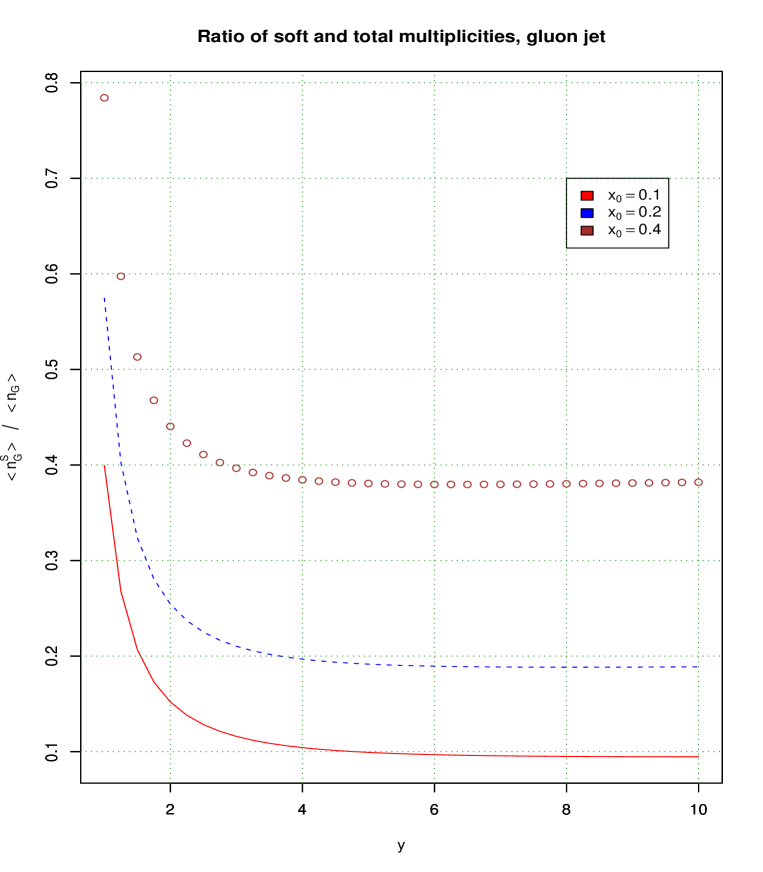
Figure 1: Energy dependence of the ratio of soft to total multiplicities in gluon jet $\langle n^{S}_{G}\rangle/\langle n_{G}\rangle$ for various cutoffs $x_{0}\,=\,0.1$ (solid line, red) $x_{0}\,=\,0.2$ (dashed line, blue) and $x_{0}=\,0.4$ (dotted line, brown).

The soft jet multiplicities behave asymptotically as the total multiplicities. Some perturbative corrections in powers of $y^{-1/2}$ (or $\gamma_{0}$) appear at lower energies. Soft multiplicities are generally proportional to their softness parameter $x_{0}$ at small $x_{0}$ with terms like $x_{0}\ln x_{0}$ appearing in some $f_{i}$. All these conclusions can be tested in experiment.

Let us note that in the fixed coupling case considered in [1] the soft jet multiplicities are proportional to the total multiplicity at all energies. The proportionality factor depends only on $x_{0}$. It implies that the dependence of their ratio at lower energies demonstrated in Fig. 1 is due to the running property of the coupling strength in QCD.

This work has been supported in part by the RFBR grants 04-02-16445, 04-02-16880, 06-02-17051.

Appendix

$$w_{1}(x_{0})\;=\;\int^{x_{0}}_{0}dx\,V(x)=\int^{x_{0}}_{0}dx\,(1-\frac{3}{2}x+x^{2}-\frac{x^{3}}{2})=x_{0}-\frac{3}{4}x_{0}^{2}+\frac{x_{0}^{3}}{3}-\frac{x_{0}^{4}}{8},$$

$$w_{2}(x_{0})\;=\;\int^{x_{0}}_{0}dx\,[\frac{\ln(1-x)}{x}-2V(x)\,\ln x(1-x)],$$

$$w_{3}(x_{0})\;=\;\int^{x_{0}}_{0}dx\,[\frac{\ln^{2}(1-x)}{x}-2V(x)\,(\ln^{2}x+\ln^{2}(1-x))],$$

$$w_{4}(x_{0})\;=\;x_{0}-x_{0}^{2}+\frac{2}{3}x_{0}^{3},$$

$$w_{5}(x_{0})\;=\;x_{0}(\ln x_{0}-1)-x_{0}^{2}(\ln x_{0}-\frac{1}{2})+2x_{0}^{3}(\frac{\ln x_{0}}{3}-\frac{1}{9}),$$

$$w_{6}(x_{0})\;=\;\frac{2}{27}x_{0}^{3}(9\ln^{2}x_{0}-3\ln x_{0}+2)-\frac{x_{0}^{2}}{2}(\ln^{2}x_{0}-\frac{1}{2}\ln x_{0}+\frac{1}{2})+x_{0}(\ln^{2}x_{0}-2\ln x_{0}+2),$$

$$w_{7}(x_{0})\;=\;\int^{x_{0}}_{0}dx\,\Phi(x)=\int^{x_{0}}_{0}(1-\frac{x}{2})dx=x_{0}-\frac{x_{0}^{2}}{4},$$

$$w_{8}(x_{0})\;=\;x_{0}(\ln x_{0}-1)-\frac{x_{0}^{2}}{4}(\ln x_{0}-\frac{1}{2}),$$

$$w_{9}(x_{0})\;=\;x_{0}(\ln^{2}x_{0}-2\ln x_{0}+2)-\frac{x_{0}^{2}}{8}[2\ln^{2}x_{0}-2\ln x_{0}+1],$$

$$w_{10}(x_{0})\;=\;\int^{x_{0}}_{0}dx\,[\Phi(x)-\frac{1}{x}]\,\ln(1-x),$$

$$w_{11}(x_{0})\;=\;\int^{x_{0}}_{0}dx\,[\Phi(x)-\frac{1}{x}]\,\ln^{2}(1-x)\,,$$

The functions $V(x)$ and $\Phi(x)$ are defined in $w_{1},w_{7}$.

References

• [1] I.M.Β Dremin, Pis’maΒ vΒ ZhETFΒ 81 (2005), 391; JETP Letters  81 (2005), 307; arXiv:hep-ph/0501203
• [2] Yu.L.Β Dokshitzer, V.A.Β Khoze, A.H.Β Mueller and S.I.Β Troyan, ”Basics of Perturbative QCD”, ed. J.Β TranΒ ThanhΒ Van, Gif-sur-Yvette, Edition Frontiers, 1991
• [3] I.M.Β Dremin, UFN  164 (1994), 785; Physics-Uspekhi  37 (1994), 715
• [4] V.A.Β Khoze, W.Β Ochs, Int.Β Journ.Β Mod.Β Phys.Β A12 (1997), 2949
• [5] I.M.Β Dremin, J.W.Β Gary, Phys.Β Rep.  349 (2001), 301
• [6] I.M.Β Dremin, A.V.Β Leonidov, UFNΒ 165 (1995), 759
• [7] A.V.Β Leonidov, UFNΒ 175 (2005), 323
• [8] A.Β Capella, I.M.Β Dremin, J.W.Β Gary, V.A.Β Nechitailo, J.Β Tran Thanh Van, Phys.Β Rev.Β D61 (2000), 074009
• [9] I.M.Β Dremin, C.S.Β Lam, V.A.Β Nechitailo, Phys.Β Rev.Β D61 (2000), 074020
• [10] I.M.Β Dremin, Phys.Β Lett.Β B313 (1993), 209