Quark contribution to the small-$x$ evolution of color dipole

Abstract

The small-$x$ deep inelastic scattering in the saturation region is governed by the non-linear evolution of Wilson-lines operators. In the leading logarithmic approximation it is given by the BK equation for the evolution of color dipoles. In the NLO the nonlinear equation gets contributions from quark and gluon loops. In this paper I calculate the quark-loop contribution to small-x evolution of Wilson lines in the NLO. It turns out that there are no new operators at the one-loop level - just as at the tree level, the high-energy scattering can be described in terms of Wilson lines. In addition, from the analysis of quark loops I find that the argument of coupling constant in the BK equation is determined by the size of the parent dipole rather than by the size of produced dipoles. These results are to be supported by future calculation of gluon loops.

I Introduction

At high energies the particles move very fast along straight lines, hence they can be described by Wilson lines $U^{\eta}(x_{\perp})$ - gauge factors ordered along straight-line classical trajectory of the particle moving with rapidity $\eta$ at the transverse impact parameter $x_{\perp}$ (for a review, see mobzor, ). For deep inelastic scattering, the propagation of a quark-antiquark pair moving along straight lines and separated by a distance in the transverse direction can be approximated by the color dipole $U(x_{\perp})U^{\dagger}(y_{\perp})$ - two Wilson lines ordered along the direction collinear to quarks’ velocity. The structure function of a hadron is then proportional to a matrix element of the color dipole operator

$${\cal U}^{\eta}(x_{\perp},y_{\perp})=1-{1\over N_{c}}{\rm Tr}\{U^{\eta}(x_{\perp})U^{\dagger\eta}(y_{\perp})\}$$ (1)

switched between the target’s states ($N_{c}=3$ for QCD). Approximately, the gluon parton density is

$$x_{B}G(x_{B},\mu^{2}=Q^{2})~{}\simeq~{}\left.\langle p|~{}{\cal U}^{\eta}(x_{\perp},0)|p\rangle\right|_{x_{\perp}^{2}=Q^{-2}}$$ (2)

where $\eta=\ln{1\over x_{B}}$ and $x_{B}={Q^{2}\over 2(p\cdot q)}$ is the Bjorken variable.

The small-x behavior of the structure functions is governed by the small-$x$ evolution of color dipolesmu94 ; nnn . For sufficiently small dipoles $x_{\perp}^{2}\sim Q^{-2}$ so $\alpha_{s}(Q)\ll$1 and we can use pQCD. At high (but not asymptotic) energies we can use the leading logarithmic approximation (LLA) where $\alpha_{s}\ll 1,~{}\alpha_{s}\ln x_{B}\sim 1$. In the LLA, the high-energy amplitudes in pQCD are described by the BFKL equationbfkl leading to the power behavior $F_{2}(x_{B})\sim x_{B}^{-12{\alpha_{s}\over\pi}\ln 2}$. However, the example of DIS from very large nuclei shows that the BFKL equation is not sufficient to describe the small-$x$ behavoir of structure functions even in the LLA. Indeed, at sufficiently large atomic number $A$ we get an additional parameter $\alpha_{s}A^{1/6}\sim 1$ which must be taken into account exactly to all orders of the expansion in this parameter. The situation is essentially semiclassical: we have $\alpha_{s}\ll 1$ and $\alpha_{s}F_{\mu\nu}\sim 1$ where $F_{\mu\nu}$ is the strong field of the nucleus gluon cloud. Thus we need the LLA in the semiclassical QCD (sQCD): $\alpha_{s}\ll 1,~{}\alpha_{s}\ln x_{B}\sim 1,~{}\alpha_{s}F_{\mu\nu}\sim 1$. This situation appears to be general for sufficiently low $x_{B}$: even for the proton, where we do not have the large parameter $A$ to start with, the power behavior of gluon parton density will lead to the huge number of partons in the target leading to the state of saturationsaturation described by Color Glass Condensate in sQCDlvmodel ; jimwalk .

The LLA evolution equation for the color dipoles is non-linearnpb96 ; yura :

$${d\over d\eta}~{}{\cal U}(x,y)~{}=~{}{\alpha_{s}N_{c}\over 2\pi^{2}}\!\int\!d^{2}z~{}{(x-y)^{2}\over(x-z)^{2}(z-y)^{2}}[{\cal U}(x,z)+{\cal U}(y,z)-{\cal U}(x,y)-{\cal U}(x,z){\cal U}(z,y)]$$ (3)

The first three terms correspond to the linear BFKL evolution and describe the parton emission while the last term is responsible for the parton annihilation. For sufficiently high $x_{B}$ the parton emission balances the parton annihilation so the partons reach the state of saturation with the characteristic transverse momentum $Q_{s}$ growing with $x_{B}$ as $e^{c\ln x_{B}}$. The argument of the coupling constant in Eq. (3) is left undetermined in the LLA, and usually it is set by hand to be $Q_{s}$. Careful analysis of this argument is very important from both theoretical and experimental points of view. From the theoretical viewpoint, we need to know whether the coupling constant is determined by the size of the original dipole $|x-y|$ or of the size of the produced dipoles $|x-z|$ and/or $|z-y|$ since we may get a very different behavior of the solutions of the equation (3) (although first numerical simulations indicate a slow dependence of the cross section on the choice of the scalescaledep ). On the experimental side, the cross section is proportional to some power of the coupling constant so the argument determines how big (or how small) is the cross section. The typical argument of $\alpha_{s}$ is the characteristic transverse momenta of the process. For high enough energies, they are believed to be of order of the saturation scale $Q_{s}$ which is $\sim 2\div 3$ GeV for the LHC collider. Thus, we see that even the difference between $\alpha(Q_{s})$ and $\alpha(2Q_{s})$ can make a huge impact on the cross section.

The argument of the coupling constant cannot be determined in the LLA so the next-to-leading order (NLO) calculation is in order. In the next-to-leading order the non-linear equation (3) looks as follows ($x,y,z..$ are the transverse coordinates)

$${d\over d\eta}~{}{\rm Tr}\{U_{x}U^{\dagger}_{y}\}~{}=~{}{1\over 2\pi^{2}}\!\int\!d^{2}z\Big{(}\alpha_{s}{(x-y)^{2}\over(x-z)^{2}(z-y)^{2}}+~{}\alpha_{s}^{2}K_{\rm NLO}(x,y,z)\Big{)}[{\rm Tr}\{U_{x}U^{\dagger}_{z}\}{\rm Tr}\{U_{z}U^{\dagger}_{y}\}-N_{c}{\rm Tr}\{U_{z}U^{\dagger}_{y}\}]$$

$$+~{}\alpha_{s}^{2}\!\int\!d^{2}zd^{2}z^{\prime}\Big{(}K_{4}(x,y,z,z^{\prime})\{U_{x},U^{\dagger}_{z^{\prime}},U_{z},U^{\dagger}_{y}\}+~{}K_{6}(x,y,z,z^{\prime})\{U_{x},U^{\dagger}_{z^{\prime}},U_{z^{\prime}},U_{z},U^{\dagger}_{z},U^{\dagger}_{y}\}\Big{)}$$ (4)

where $K_{\rm NLO}$ is the next-to-leading order correction to the dipole kernel and $K_{4}$ and $K_{6}$ are the coefficients in front of the (tree) four- and six-Wilson line operators with arbitrary white arrangements of color indices. Note that $K_{\rm NLO}$ must describe the non-forward NLO BFKL contribution found recently in Ref. nfnlobfkl, . (The contribution $\sim K_{6}$ proportional to six Wilson-line operators the was obtained in Ref. balbel, ). The calculation of the quark part of the kernel is performed in the present paper and the last remaining part of Eq. (4) - the calculation of the gluon part of $K_{\rm NLO}$ and $K_{4}$ - is in progress.

It should be mentioned that NLO result does not lead automatically to the argument of coupling constant in front of the leading term in Eq. 4. In order to get this argument, we can use the renormalon-based approachrenormalons : first we get the quark part of the running coupling constant coming from the bubble chain of quark loops and then make a conjecture that the gluon part of the $\beta$-function will follow that pattern (see the discussion in Refs blm, ; braunbeneke94, ).

As we demonstrate below, the result is that the value of coupling constant is determined by the size of the original dipole rather than the size of the produced dipoles:

$${d\over d\eta}~{}{\cal U}(x,y)~{}=~{}{\alpha_{s}((x-y)^{2})N_{c}\over 2\pi^{2}}\!\int\!d^{2}z~{}{(x-y)^{2}\over(x-z)^{2}(z-y)^{2}}[{\cal U}(x,z)+{\cal U}(y,z)-{\cal U}(x,y)-{\cal U}(x,z){\cal U}(z,y)]+...$$ (5)

The paper is organized as follows. In Sect. 2 I recall the derivation of the BK equation in the leading order in $\alpha_{s}$. In Sect. 3, which is central to the paper, I calculate the quark contribution to the small-$x$ evolution kernel of Wilson-line operators. In Sect. 4 I present the arguments that the coupling constant in the BK equation is determined by the size $(x-y)_{\perp}$ of the parent dipole. The light-cone expansion of the quark-loop propagator is performed in the Appendix.

II Derivation of the BK equation

Before discussion of the small-x evolution of color dipole in the next-to-leading approximation it is instructive to recall the derivation of the leading-order (BK) evolution equation. As discussed in the Introduction, the dependence of the structure functions on $x_{B}$ comes from the dependence of Wilson-line operators

$$U^{\eta}(x_{\perp})={\rm Pexp}\Big{\{}ig\int_{-\infty}^{\infty}\!\!du~{}p^{\eta}_{\mu}~{}A^{\mu}(up^{\eta}+x_{\perp})\Big{\}},~{}~{}~{}~{}p^{\eta}\equiv p_{1}+e^{-\eta}p_{2}$$ (6)

on the slope of the supporting line. Here $p_{1}$ and $p_{2}$ are the light-like vectors such that $q=p_{1}-x_{B}p_{2}$ and $p=p_{2}+{m^{2}\over s}p_{1}$ where $p$ is the momentum of the target and $m$ is the mass. Throughout the paper, we use the Sudakov variables $p=\alpha p_{1}+\beta p_{2}+p_{\perp}$ and the notations $x_{\bullet}\equiv x_{\mu}p_{1}^{\mu}$ and $x_{\ast}\equiv x_{\mu}p_{2}^{\mu}$ related to the light-cone coordinates: $x_{\ast}=x^{+}\sqrt{s/2},~{}x_{\bullet}=x^{-}\sqrt{s/2}$.

To find the evolution of the color dipole (1) with respect to the slope of the Wilson lines in the leading log approximation, we consider the matrix element of the color dipole between (arbitrary) target states and integrate over the gluons with rapidities $\eta_{1}>\eta>\eta_{2}=\eta_{1}-\Delta\eta$ leaving the gluons with $\eta<\eta_{2}$ as the background field (to be integrated over later). In the frame of gluons with $\eta\sim\eta_{1}$ the fields with $\eta<\eta_{2}$ shrink to a pancake and we obtain the four diagrams shown in Fig. 1

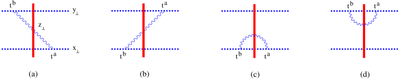
Figure 1: Leading-order diagrams for the small-$x$ evolution of color dipole.

The (background-Feynman) gluon propagator in a shock-wave external field has the formnpb96 ; prd99

$$\langle A^{a}_{\mu}(x)A^{b}_{\nu}(y)\rangle~{}=~{}\theta(x_{\ast}y_{\ast})(x|{g_{\mu\nu}\delta^{ab}\over i(p^{2}+i\epsilon)}|y)~{}$$ (7)

$$-~{}\theta(x_{\ast})\theta(-y_{\ast})\!\int_{0}^{\infty}\!{\textstyle d}\lower 0.12915pt\hbox{\kern-3.99994pt${}^{\scriptstyle-}$}\kern-0.80002pt{}\alpha~{}{e^{-i\alpha(x-y)_{\bullet}}\over 4\alpha^{2}}(x_{\perp}|e^{-i{p_{\perp}^{2}\over\alpha s}x_{\ast}}\Big{[}2\alpha g_{\mu\nu}U+{4\over s}(i\partial_{\mu}p_{2\nu}U-p_{2\mu}i\partial_{\nu}U)-{4p_{2\mu}p_{2\nu}\over\alpha s^{2}}\partial_{\perp}^{2}U\Big{]}e^{i{p_{\perp}^{2}\over\alpha s}y_{\ast}}|y_{\perp})^{ab}$$

$$-~{}\theta(-x_{\ast})\theta(y_{\ast})\!\int_{0}^{\infty}\!{\textstyle d}\lower 0.12915pt\hbox{\kern-3.99994pt${}^{\scriptstyle-}$}\kern-0.80002pt{}\alpha~{}{e^{i\alpha(x-y)_{\bullet}}\over 4\alpha^{2}}(x_{\perp}|e^{-i{p_{\perp}^{2}\over\alpha s}x_{\ast}}\Big{[}2\alpha g_{\mu\nu}U^{\dagger}-{4\over s}(i\partial_{\mu}U^{\dagger}p_{2\nu}-p_{2\mu}i\partial_{\nu}U^{\dagger})-{4p_{2\mu}p_{2\nu}\over\alpha s^{2}}\partial_{\perp}^{2}U^{\dagger}\Big{]}e^{i{p_{\perp}^{2}\over\alpha s}y_{\ast}}|y_{\perp})^{ab}$$

where $\partial_{\perp}^{2}\equiv-\partial_{i}\partial^{i}$. Hereafter use Schwinger’s notations $(x|F(p)|y)\equiv\int\!{\textstyle d}\lower 0.12915pt\hbox{\kern-3.99994pt${}^{\scriptstyle-}$}\kern-0.80002pt{}p~{}F(p)~{}e^{-ip\cdot(x-y)}$ and $(x_{\perp}|F(p_{\perp})|y)\equiv\int\!{\textstyle d}\lower 0.12915pt\hbox{\kern-3.99994pt${}^{\scriptstyle-}$}\kern-0.80002pt{}p~{}e^{i(p,x-y)_{\perp}}$ ( the scalar product of the four-dimensional vectors in our notations is $x\cdot y={2\over s}(x_{\ast}y_{\bullet}+x_{\ast}y_{\bullet})-(x,y)_{\perp}$). We obtain

$$\Big{\{}\!\int_{0}^{\infty}\!du\int^{0}_{-\infty}\!dv~{}A^{a}_{\bullet}(up^{\eta_{1}}+x_{\perp})A^{b}_{\bullet}(vp^{\eta_{1}}+y_{\perp})\Big{\}}_{\rm Fig.\ref{bkevol}a}$$

$$=~{}-2\alpha_{s}\int_{e^{-\eta_{2}}}^{\infty}\!{d\alpha\over\alpha}(x_{\perp}|{1\over p_{\perp}^{2}+\alpha^{2}e^{-2\eta_{1}}s}\partial_{\perp}^{2}U^{ab}{1\over p_{\perp}^{2}+\alpha^{2}e^{-2\eta_{1}}s}|y_{\perp})$$ (8)

Formally, the integral over $\alpha$ diverges at the lower limit, but since we integrate over the rapidities $\eta>\eta_{2}$ we get in the LLA

$$\Big{\{}\!\int_{0}^{\infty}\!du\int^{0}_{-\infty}\!dv~{}A^{a}_{\bullet}(up_{\eta}+x_{\perp})A^{b}_{\bullet}(vp_{\eta}+y_{\perp})\Big{\}}_{\rm Fig.\ref{bkevol}a}$$

$$=~{}-2\alpha_{s}\Delta\eta(x_{\perp}|{1\over p_{\perp}^{2}}\partial_{\perp}^{2}U^{ab}{1\over p_{\perp}^{2}}|y_{\perp})~{}=~{}-2\alpha_{s}\Delta\eta\!\int\!d^{2}z_{\perp}(x_{\perp}|{p_{i}\over p_{\perp}^{2}}|z_{\perp})(2U_{z}-U_{x}-U_{y})^{ab}(z_{\perp}|{p_{i}\over p_{\perp}^{2}}|y_{\perp})$$ (9)

and therefore

$$\Big{\{}U_{x}\otimes U^{\dagger}_{y}\Big{\}}_{\rm Fig.\ref{bkevol}a}^{\eta_{1}}$$

$$=~{}-{\alpha_{s}\over 2\pi^{2}}\Delta\eta~{}\{t^{a}U_{x}\otimes t^{b}U^{\dagger}_{y}\}^{\eta_{2}}\!\int\!d^{2}z_{\perp}{(x-z,y-z)_{\perp}\over(x-z)_{\perp}^{2}(y-z)_{\perp}^{2}}(2U_{z}^{\eta_{2}}-U_{x}^{\eta_{2}}-U_{y}^{\eta_{2}})^{ab}$$ (10)

The contribution of the diagram in Fig. 1b is obtained from Eq. (10) by the replacement $t^{a}U_{x}\otimes t^{b}U^{\dagger}_{y}\rightarrow U_{x}t^{b}\otimes U^{\dagger}_{y}t^{a}$, $x\leftrightarrow y$ and the two remaining diagrams are obtained from Eq. 9 by taking $y=x$ (Fig. 1c) and $x=y$ (Fig. 1d). Finally, one obtains

$$\Big{\{}U_{x}\otimes U^{\dagger}_{y}\Big{\}}_{\rm Fig.\ref{bkevol}}^{\eta_{1}}~{}=~{}-{\alpha_{s}\Delta\eta\over 2\pi^{2}}\{t^{a}U_{x}\otimes t^{b}U^{\dagger}_{y}+U_{x}t^{b}\otimes U^{\dagger}_{y}t^{a}\}^{\eta_{2}}\!\int\!d^{2}z_{\perp}{(x-z,y-z)_{\perp}\over(x-z)_{\perp}^{2}(y-z)_{\perp}^{2}}(2U_{z}^{\eta_{2}}-U_{x}^{\eta_{2}}-U_{y}^{\eta_{2}})^{ab}$$

$$+~{}{\alpha_{s}\Delta\eta\over\pi^{2}}\{t^{a}U_{x}t^{b}\otimes U^{\dagger}_{y}\}^{\eta_{2}}\!\int\!{d^{2}z_{\perp}\over(x-z)_{\perp}^{2}}(U_{z}^{\eta_{2}}-U_{x}^{\eta_{2}})^{ab}+{\alpha_{s}\Delta\eta\over\pi^{2}}\{U_{x}\otimes t^{b}U^{\dagger}_{y}t^{a}\}^{\eta_{2}}\!\int\!{d^{2}z_{\perp}\over(y-z)_{\perp}^{2}}(U_{z}^{\eta_{2}}-U_{y}^{\eta_{2}})^{ab}$$ (11)

For the color dipole (1) one easily gets the BK equation (3).

III Quark contribution to the NLO BK kernel

III.1 Quark loop in the momentum representation

There are two types of quark contribution in the NLO: with quarks in the loop interacting with the shock wave (see Fig. 2a) or without ( Fig. 2b). (In principle, there could have been the contribution coming from the quark loop which lies entirely in the shock wave, but we will demonstrate below that it vanishes).

The quark propagator in a shock-wave background has the form npb96 :

$$\psi(x)\bar{\psi}(y)~{}=~{}\theta(x_{\ast}y_{\ast})(x|{i\not\!p\over p^{2}+i\epsilon}|y)$$

$$+~{}\theta(x_{\ast})\theta(-y_{\ast})\!\int_{0}^{\infty}\!{{\textstyle d}\lower 0.12915pt\hbox{\kern-3.99994pt${}^{\scriptstyle-}$}\kern-0.80002pt{}\alpha\over 2\alpha^{2}s}~{}e^{-i\alpha(x-y)_{\bullet}}~{}(x_{\perp}|(\alpha\hat{p}_{1}+\hat{p}_{\perp})e^{-i{p_{\perp}^{2}\over\alpha s}x_{\ast}}\hat{p}_{2}Ue^{i{p_{\perp}^{2}\over\alpha s}y_{\ast}}(\alpha\hat{p}_{1}+\hat{p}_{\perp})|y_{\perp})$$

$$-~{}\theta(-x_{\ast})\theta(y_{\ast})\!\int_{-\infty}^{0}{{\textstyle d}\lower 0.12915pt\hbox{\kern-3.99994pt${}^{\scriptstyle-}$}\kern-0.80002pt{}\alpha\over 2\alpha^{2}s}~{}e^{-i\alpha(x-y)_{\bullet}}~{}(x_{\perp}|(\alpha\hat{p}_{1}+\hat{p}_{\perp})e^{-i{p_{\perp}^{2}\over\alpha s}x_{\ast}}\hat{p}_{2}U^{\dagger}e^{i{p_{\perp}^{2}\over\alpha s}y_{\ast}}(\alpha\hat{p}_{1}+\hat{p}_{\perp})|y_{\perp})$$ (12)

Multiplying two propagators one gets at $x_{\ast}>0,y_{\ast}<0$

$$\bar{\psi}t^{a}\!\not\!p_{1}\psi(x)\bar{\psi}(y)\!\not\!p_{1}\psi(y)~{}=~{}$$

$$=~{}\!\int_{0}^{\infty}\!{{\textstyle d}\lower 0.12915pt\hbox{\kern-3.99994pt${}^{\scriptstyle-}$}\kern-0.80002pt{}\alpha\over 16\pi\alpha^{3}}\!\int_{0}^{1}\!{dv\over\bar{v}^{2}v^{2}}~{}e^{-i\alpha(x-y)_{\bullet}}~{}{\rm tr}{\rm Tr}(x_{\perp}|\not\!p_{\perp}e^{-i{p_{\perp}^{2}\over\alpha vs}x_{\ast}}Ue^{i{p_{\perp}^{2}\over\alpha vs}y_{\ast}}\!\not\!p_{\perp}|y_{\perp})~{}t^{b}(y_{\perp}|\!\not\!p_{\perp}e^{i{p_{\perp}^{2}\over\alpha\bar{v}s}y_{\ast}}U^{\dagger}e^{i{p_{\perp}^{2}\over\alpha\bar{v}s}y_{\ast}}\!\not\!p_{\perp}|x_{\perp})$$ (13)

where tr stands for the trace over spinor indices. Therefore the quark-loop contribution to the gluon propagator is

$$\langle A^{a}_{\bullet}(x)A^{b}_{\bullet}(y)\rangle$$

$$=~{}2\alpha^{2}_{s}n_{f}\int_{0}^{\infty}\!{d\alpha\over\alpha^{3}}\!\int\!d^{2}zd^{2}z^{\prime}\!\int{\textstyle d}\lower 0.12915pt\hbox{\kern-3.99994pt${}^{\scriptstyle-}$}\kern-0.80002pt{}^{2}k_{1}{\textstyle d}\lower 0.12915pt\hbox{\kern-3.99994pt${}^{\scriptstyle-}$}\kern-0.80002pt{}^{2}k^{\prime}_{1}{\textstyle d}\lower 0.12915pt\hbox{\kern-3.99994pt${}^{\scriptstyle-}$}\kern-0.80002pt{}^{2}k_{2}{\textstyle d}\lower 0.12915pt\hbox{\kern-3.99994pt${}^{\scriptstyle-}$}\kern-0.80002pt{}^{2}k^{\prime}_{2}~{}e^{i(k_{1},x-z)_{\perp}+i(k^{\prime}_{1},x-z^{\prime})_{\perp}-i(k_{2},y-z)_{\perp}-i(k^{\prime}_{2},y-z^{\prime})_{\perp}}$$

$${\rm Tr}\{t^{a}U_{z}t^{b}U^{\dagger}_{z^{\prime}}\}\int_{0}^{1}\!dv~{}{(k_{1},k_{2})(k^{\prime}_{1},k^{\prime}_{2})+(k_{1},k^{\prime}_{1})(k_{2},k^{\prime}_{2})-(k_{1},k^{\prime}_{2})(k^{\prime}_{1},k_{2})\over[(k_{1}+k^{\prime}_{1})^{2}\bar{v}v-k^{2}_{1}\bar{v}-{k^{\prime}_{1}}^{2}v][(k_{2}+k^{\prime}_{2})^{2}\bar{v}v-k^{2}_{2}\bar{v}-{k^{\prime}_{2}}^{2}v]}$$

$$\times~{}\Big{[}e^{-i{(k_{1}+k^{\prime}_{1})_{\perp}^{2}\over\alpha s}x_{\ast}}-e^{-i\Big{(}{k_{1}^{2}\over v}+{{k^{\prime}_{1}}^{2}\over\bar{v}}\Big{)}{x_{\ast}\over\alpha s}}\Big{]}\Big{[}e^{i{(k_{2}+k^{\prime}_{2})_{\perp}^{2}\over\alpha s}y_{\ast}}-e^{i({k_{2}^{2}\over v}+{{k^{\prime}_{2}}^{2}\over\bar{v}}){y_{\ast}\over\alpha s}}\Big{]}$$ (14)

and one obtains the contribution of the diagram in Fig. 2a in the form

$$\Big{\{}\!\int_{0}^{\infty}\!du\int^{0}_{-\infty}\!dv~{}A^{a}_{\bullet}(up_{1}+x_{\perp})A^{b}_{\bullet}(vp_{1}+y_{\perp})\Big{\}}_{\rm Fig.\ref{kvloop1}a}$$

$$=~{}-8\alpha^{2}_{s}n_{f}\int_{0}^{\infty}\!{d\alpha\over\alpha}\!\int\!dzdz^{\prime}\!\int{\textstyle d}\lower 0.12915pt\hbox{\kern-3.99994pt${}^{\scriptstyle-}$}\kern-0.80002pt{}^{2}k_{1}{\textstyle d}\lower 0.12915pt\hbox{\kern-3.99994pt${}^{\scriptstyle-}$}\kern-0.80002pt{}^{2}k^{\prime}_{1}{\textstyle d}\lower 0.12915pt\hbox{\kern-3.99994pt${}^{\scriptstyle-}$}\kern-0.80002pt{}^{2}k_{2}{\textstyle d}\lower 0.12915pt\hbox{\kern-3.99994pt${}^{\scriptstyle-}$}\kern-0.80002pt{}^{2}k^{\prime}_{2}~{}e^{i(k_{1},x-z)_{\perp}+i(k^{\prime}_{1},x-z^{\prime})_{\perp}-i(k_{2},y-z)_{\perp}-i(k^{\prime}_{2},y-z^{\prime})_{\perp}}$$

$${\rm Tr}\{t^{a}U_{z}t^{b}U^{\dagger}_{z^{\prime}}\}\int_{0}^{1}\!dv~{}{(k_{1},k_{2})(k^{\prime}_{1},k^{\prime}_{2})+(k_{1},k^{\prime}_{1})(k_{2},k^{\prime}_{2})-(k_{1},k^{\prime}_{2})(k^{\prime}_{1},k_{2})\over(k_{1}+k^{\prime}_{1})^{2}(k_{2}+k^{\prime}_{2})^{2}(k^{2}_{1}v+{k^{\prime}_{1}}^{2}\bar{v})(k^{2}_{2}v+{k^{\prime}_{2}}^{2}\bar{v})}$$ (15)

where $n_{f}$ is a number of light quarks ($n_{f}=3$ for the momenta $Q_{s}\sim 1\div 2$ GeV) and Tr stands for the trace over color indices. The variable $v$ is the fraction of the gluon’s momentum $\alpha$ carried by the quark.

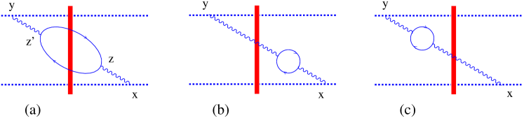
Figure 2: Quark-loop contribution to the gluon propagator in a shock-wave background .

To calculate this diagram we use the dimensional regularization and change the dimension of the transverse space to $d=2-2\epsilon$. The calculation yields

$${\rm Tr}\{U_{x}U^{\dagger}_{y}\}_{\rm Fig.\ref{kvloop1}a}$$

$$=~{}-{4\alpha^{2}_{s}\over\pi}n_{f}\Delta\eta{\rm Tr}\{t^{a}U_{x}t^{b}U^{\dagger}_{y}\}\int\!{\textstyle d}\lower 0.12915pt\hbox{\kern-3.99994pt${}^{\scriptstyle-}$}\kern-0.80002pt{}^{d}p~{}{\textstyle d}\lower 0.12915pt\hbox{\kern-3.99994pt${}^{\scriptstyle-}$}\kern-0.80002pt{}^{d}q~{}{\textstyle d}\lower 0.12915pt\hbox{\kern-3.99994pt${}^{\scriptstyle-}$}\kern-0.80002pt{}^{d}q^{\prime}~{}{e^{i(p,x)_{\perp}-i(p-q-q^{\prime},y)_{\perp}}\over p^{2}(p-q-q^{\prime})^{2}}\!\int_{0}^{1}\!dvdu~{}\Bigg{[}-(q+q^{\prime})^{2}{\bar{u}u\Gamma(\epsilon)\mu^{2\epsilon}\over(P^{2}\bar{v}v+Q^{2}\bar{u}u)^{\epsilon}}$$

$$+~{}{\Gamma(1+\epsilon)\mu^{2\epsilon}\over(P^{2}\bar{v}v+Q^{2}\bar{u}u)^{1+\epsilon}}\Big{\{}P^{2}[\bar{v}v(q,q^{\prime})-\bar{u}uQ^{2}+2\bar{u}u\bar{v}v(q^{2}+{q^{\prime}}^{2})]-2\bar{u}u\bar{v}v(P,q)(P,q^{\prime})$$

$$+~{}\bar{u}u(1-2u)[\bar{v}v(q,q^{\prime})(P,q+q^{\prime})+\bar{v}q^{2}(P,q^{\prime})+v{q^{\prime}}^{2}(P,q)]+\bar{u}^{2}u^{2}Q^{2}(q+q^{\prime})^{2}\Big{\}}\Bigg{]}{\rm Tr}\{t^{a}U(q)t^{b}U^{\dagger}(q^{\prime})\}$$ (16)

where $P\equiv p-(q+q^{\prime})u$, $Q^{2}=q_{\perp}^{2}\bar{v}+{q^{\prime}}_{\perp}^{2}v$ and we use the notation $\int\!{\textstyle d}\lower 0.12915pt\hbox{\kern-3.99994pt${}^{\scriptstyle-}$}\kern-0.80002pt{}^{d}p_{\perp}\equiv\!\int\!{dp_{\perp}\over(2\pi)^{d}}$.

The contribution of two diagrams in Fig. 2b,c is

$$2n_{f}\alpha^{2}_{s}\Delta\eta{\rm tr}\{t^{a}U_{x}t^{b}U^{\dagger}_{y}\}{\mu^{2\epsilon}\over\pi}B(2-\epsilon,2-\epsilon)(x_{\perp}|{1\over p_{\perp}^{2}}\Big{\{}{\Gamma(\epsilon)\over(p_{\perp}^{2})^{\epsilon}},\partial_{\perp}^{2}U^{ab}\Big{\}}{1\over p_{\perp}^{2}}|y_{\perp})$$ (17)

where $B(a,b)=\Gamma(a)\Gamma(b)/\Gamma(a+b)$. The contribution of diagrams in Fig. 3 is obtained from the sum of Eq. (16) and (17) by the $x\leftrightarrow y$ replacement in the coefficient in front of ${\rm tr}\{t^{a}U_{x}t^{b}U^{\dagger}_{y}\}$

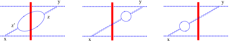
Figure 3: .

and the contribution of the diagram in Fig. 4 by taking $y\rightarrow x$ in this coefficient and changing the sign.

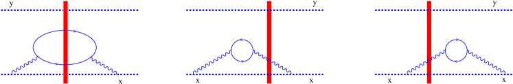
Figure 4: .

Similarly, the diagram in Fig. 5 is obtained by taking $x\rightarrow y$.

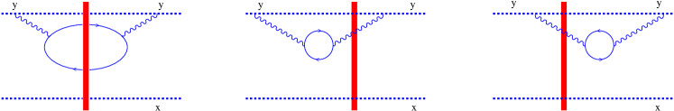
Figure 5: .

The sum of all diagrams has the form

$${\rm Tr}\{U_{x}U^{\dagger}_{y}\}~{}=-{\alpha^{2}_{s}\over\pi}n_{f}\Delta\eta{\rm Tr}\{t^{a}U_{x}t^{b}U^{\dagger}_{y}\}$$ (18)

$$\times~{}\Bigg{(}\int\!{{\textstyle d}\lower 0.12915pt\hbox{\kern-3.99994pt${}^{\scriptstyle-}$}\kern-0.80002pt{}^{d}p~{}{\textstyle d}\lower 0.12915pt\hbox{\kern-3.99994pt${}^{\scriptstyle-}$}\kern-0.80002pt{}^{d}q~{}{\textstyle d}\lower 0.12915pt\hbox{\kern-3.99994pt${}^{\scriptstyle-}$}\kern-0.80002pt{}^{d}q^{\prime}\over p^{2}(p-q-q^{\prime})^{2}}~{}(e^{i(p,x)_{\perp}}-e^{i(p,y)_{\perp}})(e^{-i(p-q-q^{\prime},x)_{\perp}}-e^{-i(p-q-q^{\prime},y)_{\perp}})\!\int_{0}^{1}\!dudv~{}\Big{[}(q+q^{\prime})^{2}{4\bar{u}u\Gamma(\epsilon)\mu^{2\epsilon}\over(P^{2}\bar{v}v+Q^{2}\bar{u}u)^{\epsilon}}$$

$$-~{}4{\Gamma(1+\epsilon)\mu^{2-d}\over(P^{2}\bar{v}v+Q^{2}\bar{u}u)^{1+\epsilon}}\Big{\{}P^{2}[\bar{v}v(q,q^{\prime})-\bar{u}uQ^{2}+2\bar{u}u\bar{v}v(q^{2}+{q^{\prime}}^{2})]-2\bar{u}u\bar{v}v(P,q)(P,q^{\prime})$$

$$+~{}\bar{u}u(1-2u)[\bar{v}v(q,q^{\prime})(P,q+q^{\prime})+\bar{v}q^{2}(P,q^{\prime})+v{q^{\prime}}^{2}(P,q)]+\bar{u}^{2}u^{2}Q^{2}(q+q^{\prime})^{2}\Big{\}}\Big{]}{\rm Tr}\{t^{a}U(q_{\perp})t^{b}U^{\dagger}(q^{\prime}_{\perp})\}$$

$$-~{}2\mu^{2\epsilon}B(2-\epsilon,2-\epsilon)\Big{[}2(x_{\perp}|{1\over p_{\perp}^{2}}\Big{\{}{\Gamma(\epsilon)\over p_{\perp}^{2\epsilon}},\partial_{\perp}^{2}U^{ab}\Big{\}}{1\over p_{\perp}^{2}}|y_{\perp})-(x_{\perp}|{1\over p_{\perp}^{2}}\Big{\{}{\Gamma(\epsilon)\over p_{\perp}^{2\epsilon}},\partial_{\perp}^{2}U^{ab}\Big{\}}{1\over p_{\perp}^{2}}|x_{\perp})$$

$$-~{}(y_{\perp}|{1\over p_{\perp}^{2}}\Big{\{}{\Gamma(\epsilon)\over p_{\perp}^{2\epsilon}},\partial_{\perp}^{2}U^{ab}\Big{\}}{1\over p_{\perp}^{2}}|y_{\perp})\Big{]}+{1\over 3\epsilon}\Big{[}2(x_{\perp}|{1\over p_{\perp}^{2}}\partial_{\perp}^{2}U^{ab}{1\over p_{\perp}^{2}}|y_{\perp})-(x_{\perp}|{1\over p_{\perp}^{2}}\partial_{\perp}^{2}U^{ab}{1\over p_{\perp}^{2}}|x_{\perp})-(y_{\perp}|{1\over p_{\perp}^{2}}\partial_{\perp}^{2}U^{ab}{1\over p_{\perp}^{2}}|y_{\perp})\Big{]}\Bigg{)}$$

where the last term $\sim{1\over 3\epsilon}$ is a counterterm calculated in the Appendix.

III.2 Quark loop inside the shock wave

Let us consider the diagram in Fig. 6 with the quark loop inside the shock wave of width $\lambda=\Delta z_{\ast}\sim{s\over m^{2}}e^{-\eta_{2}}$ where $m^{2}$ is some characteristic mass scale of order of $Q^{2}$.

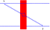
Figure 6: Quark loop inside the shock wave .

From the form of the perturbative propagator

$$(z|{1\over p^{2}+i\epsilon}|z^{\prime})={s\over 8\pi x_{\ast}}\!\int_{0}^{\infty}\!{{\textstyle d}\lower 0.12915pt\hbox{\kern-3.99994pt${}^{\scriptstyle-}$}\kern-0.80002pt{}\alpha\over\alpha}e^{-i\alpha(z-z^{\prime})_{\bullet}-i{(z-z^{\prime})_{\perp}^{2}\over 4(z-z^{\prime})_{\ast}}\alpha s}$$

we see that the characteristic transverse scale inside the shock wave is

$$(z-z^{\prime})_{\perp}^{2}\sim{\lambda\over\alpha s}\simeq m^{-2}{e^{-\eta_{2}}\over\alpha}\ll m^{-2}$$ (19)

and therefore the contribution of the diagram in Fig. 6 reduces to the contribution of some operator local in the transverse space. By dimensional arguments, this local operator must have the same twist as the operator describing the interaction of the gluon with the shock wave at the tree level. In the leading order in $\alpha_{s}$, the vertex of interaction of gluon with the shock-wave field is proportional to

$$\partial_{\perp}^{2}U~{}=~{}-ig[DG]+2g^{2}[GG]$$ (20)

where

$$[DG]\equiv\int\!du~{}[\infty p_{1},up_{1}]_{x}D^{i}G_{i\bullet}(up_{1}+x_{\perp})[up_{1},-\infty p_{1}]_{x}$$ (21)

$$[GG]\equiv\int\!dudv~{}\theta(u-v)~{}[\infty p_{1},up_{1}]_{x}G_{\bullet i}(up_{1}+x_{\perp})[up_{1},vp_{1}]_{x}G_{\bullet}^{~{}i}(vp_{1}+x_{\perp})[vp_{1},-\infty p_{1}]_{x}$$

These operators have twist 2 so a possible local operator describing the gluon interaction with the shock wave at the one-loop level must also be of twist 2. To find this local operator, we consider (the quark loop contribution to) the color dipole ${\rm tr}\{U_{x}U^{\dagger}_{y}\}$ at small at $(x-y)_{\perp}^{2}\rightarrow 0$ and compare the expansion of the contribution of the diagrams in Fig. 2 to the exact calculation of the light-cone expansion of ${\rm tr}\{U_{x}U^{\dagger}_{y}\}$ in QCD (up to twist-2 level), see Fig. 7.

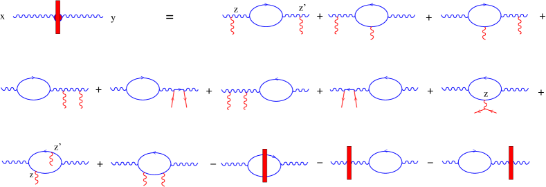
Figure 7: A possible local contibution coming from the quark loop inside the shock wave .

The first step is the light-cone expansion of the sum of the diagrams in the in Figs. 2- 5 in the shock-wave background. The light-cone expansion of Eq. (18) at $x_{\perp}\rightarrow y_{\perp}$ starts with terms quadratic in $q$($q^{\prime}$). They lead to the operators $\partial^{2}U_{x}$ and $\partial_{i}U_{x}\partial_{i}U^{\dagger}_{x}$ (in the leading order we do not distinguish between $U_{x}$ and $U_{y}$):

$${\rm Tr}\{\partial_{i}U_{x}\partial_{i}U^{\dagger}_{y}\}\stackrel{{\scriptstyle x\rightarrow y_{\perp}}}{{=}}{\alpha^{2}_{s}\over\pi}n_{f}\Delta\eta U_{x}^{ab}~{}\Bigg{[}{4\over 3}\mu^{2-d}B(1-\epsilon,1-\epsilon)(x_{\perp}|\Big{(}[3-{1\over\epsilon}]\delta_{ij}-{p_{i}p_{j}\over p_{\perp}^{2}}\Big{)}{\Gamma(1+\epsilon)\over(p_{\perp}^{2})^{1+\epsilon}}|y_{\perp}){\rm Tr}\{t^{a}\partial_{i}U_{x}t^{b}\partial_{j}U^{\dagger}_{x}\}$$

$$+~{}4\mu^{2-d}B(2-\epsilon,2-\epsilon)(x_{\perp}|{\Gamma(\epsilon)\over(p_{\perp}^{2})^{1+\epsilon}}|y_{\perp})\partial_{\perp}^{2}U_{x}^{ab}-{1\over 3\epsilon}(x_{\perp}|{1\over p_{\perp}^{2}}|y_{\perp})\partial_{\perp}^{2}U_{x}^{ab}\Bigg{]}$$

$$=~{}{\alpha^{2}_{s}\over\pi^{2}}n_{f}\Delta\eta~{}\Bigg{\{}{1\over 6N_{c}}\mu^{2\epsilon}B(1-\epsilon,1-\epsilon)\Big{[}\Big{(}{1\over\epsilon}-3+{1\over 2(1+\epsilon)}\Big{)}\delta_{ij}+{2\epsilon\over(1+\epsilon)}{\Delta_{i}\Delta_{j}\over\Delta_{\perp}^{2}}\Big{]}{\Gamma(-2\epsilon)\over(\Delta_{\perp}^{2})^{-2\epsilon}}{\rm Tr}\{\partial_{i}U_{x}\partial_{j}U^{\dagger}_{x}\}$$

$$+~{}{\mu^{2\epsilon}\over\epsilon}B(2-\epsilon,2-\epsilon){\Gamma(-2\epsilon)\over(\Delta_{\perp}^{2})^{-2\epsilon}}-{1\over 12\epsilon}{\Gamma(-\epsilon)\over(\Delta_{\perp}^{2})^{-\epsilon}}\Big{]}U_{x}^{an}\partial_{\perp}^{2}U_{x}^{ab}\Bigg{\}}$$ (22)

The expression (22) should be compared to the light-cone expansion of the quark-loop part of the gluon propagator in an external field (see Fig. 7) performed in the Appendix. A typical term of the light-cone expansion has the form:

$$A^{a}_{\bullet}(x_{\ast},x_{\perp})A^{b}_{\bullet}(y_{\ast},y_{\perp})~{}=~{}{ig^{3}\over 16\pi^{2}}B(2-\epsilon,2-\epsilon)\!\int_{0}^{\infty}\!{{\textstyle d}\lower 0.12915pt\hbox{\kern-3.99994pt${}^{\scriptstyle-}$}\kern-0.80002pt{}\alpha\over\alpha^{3}}\Big{(}{4i\over\alpha s}\Big{)}^{\epsilon}\Big{(}-{i\alpha s\over 4\pi\Delta_{\ast}}\Big{)}^{1-\epsilon}e^{i{\Delta_{\perp}^{2}\over 4\Delta_{\ast}}\alpha s}$$ (23)

$$\times~{}\Bigg{[}-ig\!\int_{y_{\ast}}^{x_{\ast}}\!\!d{2\over s}z_{\ast}~{}{1\over\epsilon}[(x-z)_{\ast}^{\epsilon}+(z-y)_{\ast}^{\epsilon}]~{}([x_{\ast},z_{\ast}]_{x}D^{i}G_{i{\bullet}}(z_{\ast},x_{\perp})[z_{\ast},z^{\prime}_{\ast}]_{x}[z_{\ast},y_{\ast}]_{x})^{ab}$$

$$+~{}g62\!\int_{y_{\ast}}^{x_{\ast}}\!\!d{2\over s}z_{\ast}\!\int_{y_{\ast}}^{z_{\ast}}\!\!d{2\over s}z^{\prime}_{\ast}~{}([x_{\ast},z_{\ast}]_{x}G_{\bullet}^{~{}i}(z_{\ast},x_{\perp})[z_{\ast},z^{\prime}_{\ast}]_{x}G_{{\bullet}i}(z^{\prime}_{\ast},x_{\perp})[z^{\prime}_{\ast},y_{\ast}]_{x})^{ab}\Big{\{}{1\over\epsilon}[(x-z)_{\ast}^{\epsilon}+(z^{\prime}-y)_{\ast}^{\epsilon}]+(z-z^{\prime})_{\ast}^{\epsilon}\Big{\}}\Bigg{]}$$

In our “external” field the characteristic distances $z_{\ast}(z^{\prime}_{\ast})$ are of the order of width of the shock wave: $z_{\ast},z^{\prime}_{\ast}\sim e^{\eta_{2}}\sqrt{s/m^{2}}$. As we shall see below, the characteristic distances $x_{\ast}$ and $y_{\ast}$ are $\sim e^{\eta_{1}}\sqrt{s/m^{2}}$ so we can neglect $z_{\ast}$ and $z^{\prime}_{\ast}$ in comparison to $x_{\ast}$ and/or $y_{\ast}$. The formula (69) simplifies to

$$A^{a}_{\bullet}(x_{\ast},x_{\perp})A^{b}_{\bullet}(y_{\ast},y_{\perp})~{}=~{}{ig^{3}\over 16\pi^{2}}B(2-\epsilon,2-\epsilon)\!\int_{0}^{\infty}\!{{\textstyle d}\lower 0.12915pt\hbox{\kern-3.99994pt${}^{\scriptstyle-}$}\kern-0.80002pt{}\alpha\over\alpha^{3}}\Big{(}{4i\over\alpha s}\Big{)}^{\epsilon}\Big{(}-{i\alpha s\over 4\pi\Delta_{\ast}}\Big{)}^{1-\epsilon}e^{i{\Delta_{\perp}^{2}\over 4\Delta_{\ast}}\alpha s}$$ (24)

$$\times~{}\Bigg{[}-ig{1\over\epsilon}\!\int_{y_{\ast}}^{x_{\ast}}\!\!d{2\over s}z_{\ast}~{}[x_{\ast}^{\epsilon}+(-y)_{\ast}^{\epsilon}]([x_{\ast},z_{\ast}]_{x}D^{i}G_{i{\bullet}}(z_{\ast},x_{\perp})[z_{\ast},z^{\prime}_{\ast}]_{x}[z_{\ast},y_{\ast}]_{x})^{ab}$$

$$+~{}g^{2}\!\int_{y_{\ast}}^{x_{\ast}}\!\!d{2\over s}z_{\ast}\!\int_{y_{\ast}}^{z_{\ast}}\!\!d{2\over s}z^{\prime}_{\ast}~{}([x_{\ast},z_{\ast}]_{x}G_{\bullet}^{~{}i}(z_{\ast},x_{\perp})[z_{\ast},z^{\prime}_{\ast}]_{x}G_{{\bullet}i}(z^{\prime}_{\ast},x_{\perp})[z^{\prime}_{\ast},y_{\ast}]_{x})^{ab}\Big{\{}{1\over\epsilon}[x_{\ast}^{\epsilon}+(-y)_{\ast}^{\epsilon}]+(z-z^{\prime})_{\ast}^{\epsilon}\Big{\}}\Bigg{]}$$

A very important observation is that the contributions proportional to

$$g^{4}n_{f}\int\!dz_{\ast}\!\int dz^{\prime}_{\ast}~{}\theta(z-z^{\prime})~{}(z-z^{\prime})^{\epsilon}G_{{\bullet}i}(z_{\ast})G_{{\bullet}i}(z^{\prime}_{\ast})$$ (25)

present in the individual diagrams in Fig. 11, cancel their sum. If it were not true, there would be an addtional contribution to the gluon propagator (7) at the $g^{4}$ level coming from the small-size (large-momenta) quark loop. Indeed, the calculations of Feynman diagrams with the propagators (7) and (12) imply that we first take limit $z_{\ast},z^{\prime}_{\ast}\rightarrow 0$ and limit $d_{\perp}\rightarrow 2$ afterwards. With such order of limits, the contribution (74) vanishes. However, the proper order of these limits is to first take $d_{\perp}\rightarrow 2$ (which will give finite expressions after adding the counterterms) and then try to impose condition that the external field is very narrow by taking the limit $z_{\ast},z^{\prime}_{\ast}\rightarrow 0$. In this case, Eq. (74) reduces to $g^{4}n_{f}[GG]$. The non-commutativity of these limits would mean that the contribution ${1\over p^{2}}[GG]{1\over p^{2}}$ should be added to the gluon propagator (7) to restore the correct result. Fortunately, the terms $\sim$ (74) cancel which means that there are no additional contributions to the gluon propagator coming from the quark loop inside the shock wave ($\equiv$ quark loop with large momenta).

Since there is no external field outside the shock wave, after cancellation of the terms $\sim(z-z^{\prime})^{\epsilon}$ we see that at $x_{\ast}y_{\ast}>0$ Eq. (24) vanishes, and at $x_{\ast}>0>y_{\ast}$ one can extend the limits of integration in the gluon operators to $\pm\infty$ and obtain

$$A^{a}_{\bullet}(x_{\ast},x_{\perp})A^{b}_{\bullet}(y_{\ast},y_{\perp})~{}=~{}{ig^{2}\over 16\pi^{2}}B(2-\epsilon,2-\epsilon)\!\int_{0}^{\infty}\!{{\textstyle d}\lower 0.12915pt\hbox{\kern-3.99994pt${}^{\scriptstyle-}$}\kern-0.80002pt{}\alpha\over\alpha^{3}}\Big{(}{4i\over\alpha s}\Big{)}^{\epsilon}\Big{(}-{i\alpha s\over 4\pi\Delta_{\ast}}\Big{)}^{1-\epsilon}e^{i{\Delta_{\perp}^{2}\over 4\Delta_{\ast}}\alpha s}$$ (26)

$$\times~{}\Bigg{[}-ig{1\over\epsilon}[x_{\ast}^{\epsilon}+(-y)_{\ast}^{\epsilon}][DG]^{ab}+~{}g^{2}[GG]^{ab}{1\over\epsilon}[x_{\ast}^{\epsilon}+(-y)_{\ast}^{\epsilon}]\Bigg{]}$$

$$=~{}{ig^{2}\over 16\pi^{2}}B(2-\epsilon,2-\epsilon)\!\int_{0}^{\infty}\!{{\textstyle d}\lower 0.12915pt\hbox{\kern-3.99994pt${}^{\scriptstyle-}$}\kern-0.80002pt{}\alpha\over\alpha^{3}}\Big{(}{4i\over\alpha s}\Big{)}^{\epsilon}\Big{(}-{i\alpha s\over 4\pi\Delta_{\ast}}\Big{)}^{1-\epsilon}e^{i{\Delta_{\perp}^{2}\over 4\Delta_{\ast}}\alpha s}{1\over\epsilon}[x_{\ast}^{\epsilon}+(-y)_{\ast}^{\epsilon}]~{}\partial_{\perp}^{2}U^{ab}_{x}$$

The light-cone expansion of gluon propagator contains only Wilson lines and their derivatives as should be expected after cancellation of the “contaminating” terms (74).

We have demonstrated in the Appendix that the light-cone expansion of the quark-loop contribution to the gluon propagator coincides with Eq. (22) as should be expected once we established the commutativity of the limits $d_{\perp}\rightarrow 2$ and $z_{\ast}(z^{\prime}_{\ast})\rightarrow 0$.

III.3 Quark loop in the coordinate representation

To calculate the integrals over momenta in Eq. (18) it is convenient to subtract (and add) ${\rm Tr}\{t^{a}U_{z}t^{b}U^{\dagger}_{z}\}$ from ${\rm Tr}\{t^{a}U_{z}t^{b}U^{\dagger}_{z^{\prime}}\}$:

$${\rm Tr}\{t^{a}U_{z}t^{b}U^{\dagger}_{z^{\prime}}\}={\rm Tr}\{t^{a}U_{z}t^{b}U^{\dagger}_{z^{\prime}}-t^{a}U_{z}t^{b}U^{\dagger}_{z}\}+{\rm Tr}\{t^{a}U_{z}t^{b}U^{\dagger}_{z}\}$$ (27)

Let us start with the last term in the r.h.s. of Eq. (27). In the momentum representation, this term corresponds to ${\rm Tr}\{t^{a}U(q)t^{b}U^{\dagger}(q^{\prime})\}\rightarrow 4\pi^{2}\delta(q^{\prime})\!\int\!dze^{i(q,z)_{\perp}}{\rm Tr}\{t^{a}U_{z}t^{b}U^{\dagger}_{z}\}=2\pi^{2}\delta(q^{\prime})U^{ab}(q)$ so we get

$$-2\alpha^{2}_{s}n_{f}\Delta\eta t^{a}U_{x}\otimes t^{b}U^{\dagger}_{y}{\mu^{2\epsilon}\over\pi}\int\!{\textstyle d}\lower 0.12915pt\hbox{\kern-3.99994pt${}^{\scriptstyle-}$}\kern-0.80002pt{}^{d}p~{}{\textstyle d}\lower 0.12915pt\hbox{\kern-3.99994pt${}^{\scriptstyle-}$}\kern-0.80002pt{}^{d}q~{}{e^{i(p,x)_{\perp}-i(p-q,y)_{\perp}}\over p^{2}(p-q)^{2}}U^{ab}(q)\!\int_{0}^{1}\!dvdu~{}\Bigg{[}-{\bar{u}uq^{2}\Gamma(\epsilon)\over[(p-qu)^{2}\bar{v}v+q^{2}\bar{v}\bar{u}u]^{\epsilon}}$$

$$+~{}{q^{2}\bar{u}u\bar{v}\Gamma(1+\epsilon)\over[(p-qu)^{2}\bar{v}v+q^{2}\bar{v}\bar{u}u]^{1+\epsilon}}\Big{\{}(p-qu)^{2}(-1+2v)+\bar{u}uq^{2}\Big{\}}\Bigg{]}$$

$$=~{}2{\alpha^{2}_{s}\over\pi}n_{f}\Delta\eta t^{a}U_{x}\otimes t^{b}U^{\dagger}_{y}\int\!{\textstyle d}\lower 0.12915pt\hbox{\kern-3.99994pt${}^{\scriptstyle-}$}\kern-0.80002pt{}^{d}p~{}{\textstyle d}\lower 0.12915pt\hbox{\kern-3.99994pt${}^{\scriptstyle-}$}\kern-0.80002pt{}^{d}q~{}{e^{i(p,x)_{\perp}-i(p-q,y)_{\perp}}\over p^{2}(p-q)^{2}}U^{ab}(q)~{}q^{2}{\Gamma(\epsilon)\over(q^{2}/\mu^{2})^{\epsilon}}B(2-\epsilon,2-\epsilon)$$ (28)

where we have used integration by parts to transform the second term in the l.h.s of this equation. Alternatively, this result can be obtained directly from Eq. (15) after the substitution (27).

For future use we need to rewrite it in Schwinger’s representation:

$$-2{\alpha^{2}_{s}\over\pi}\mu^{2-d}n_{f}\Delta\eta\{t^{a}U_{x}\otimes t^{b}U^{\dagger}_{y}\}(x|{1\over p^{2}}\Big{(}{\Gamma(\epsilon)\over(-\partial^{2})^{\epsilon}}\partial_{\perp}^{2}U^{ab}\Big{)}{1\over p^{2}}|y)B(2-\epsilon,2-\epsilon)$$ (29)

The contribution coming from the first term in Eq. (27) is UV-finite. To calculate it in coordinate representation it is convenient to return back to the original expression

$$-8\alpha^{2}_{s}n_{f}\Delta\eta t^{a}U_{x}\otimes t^{b}U^{\dagger}_{y}\int{\textstyle d}\lower 0.12915pt\hbox{\kern-3.99994pt${}^{\scriptstyle-}$}\kern-0.80002pt{}^{2}k_{1}{\textstyle d}\lower 0.12915pt\hbox{\kern-3.99994pt${}^{\scriptstyle-}$}\kern-0.80002pt{}^{2}k^{\prime}_{1}{\textstyle d}\lower 0.12915pt\hbox{\kern-3.99994pt${}^{\scriptstyle-}$}\kern-0.80002pt{}^{2}k_{2}{\textstyle d}\lower 0.12915pt\hbox{\kern-3.99994pt${}^{\scriptstyle-}$}\kern-0.80002pt{}^{2}k^{\prime}_{2}~{}e^{i(k_{1},x-z)_{\perp}+i(k^{\prime}_{1},x-z^{\prime})_{\perp}-i(k_{,}y-z)_{\perp}-i(k^{\prime}_{2},y-z^{\prime})_{\perp}}$$

$${\rm Tr}\{t^{a}U_{z}t^{b}U^{\dagger}_{z^{\prime}}-t^{a}U_{z}t^{b}U^{\dagger}_{z}\}\int_{0}^{1}du~{}{(k_{1},k_{2})(k^{\prime}_{1},k^{\prime}_{2})+(k_{1},k^{\prime}_{1})(k_{2},k^{\prime}_{2})-(k_{1},k^{\prime}_{2})(k^{\prime}_{1},k_{2})\over(k_{1}+k^{\prime}_{1})^{2}(k_{2}+k^{\prime}_{2})^{2}(k^{2}_{1}u+{k^{\prime}_{1}}^{2}\bar{u})(k^{2}_{2}u+{k^{\prime}_{2}}^{2}\bar{u})}$$

and use the formulas

$$\int{\textstyle d}\lower 0.12915pt\hbox{\kern-3.99994pt${}^{\scriptstyle-}$}\kern-0.80002pt{}^{d}k_{1}{\textstyle d}\lower 0.12915pt\hbox{\kern-3.99994pt${}^{\scriptstyle-}$}\kern-0.80002pt{}^{d}k_{2}~{}{(k_{1},k_{2})e^{i(k_{1},x_{1})+i(k_{2},x_{2})}\over(k_{1}+k_{2})^{2}(k_{1}^{2}\bar{u}+k_{2}^{2}u)}~{}=~{}{1\over 4\pi^{2}(x_{1}-x_{2})^{2}}\Big{[}1-{(x_{1},x_{2})\over x_{1}^{2}u+x_{2}^{2}\bar{u}}\Big{]}+O(d-2)$$

$$\int{\textstyle d}\lower 0.12915pt\hbox{\kern-3.99994pt${}^{\scriptstyle-}$}\kern-0.80002pt{}^{d}k_{1}{\textstyle d}\lower 0.12915pt\hbox{\kern-3.99994pt${}^{\scriptstyle-}$}\kern-0.80002pt{}^{d}k_{2}~{}{k_{1i}k_{2j}-i\leftrightarrow j\over(k_{1}+k_{2})^{2}(k_{1}^{2}\bar{u}+k_{2}^{2}u)}~{}e^{i(k_{1},x_{1})+i(k_{2},x_{2})}~{}=~{}-{x_{1i}x_{2j}-i\leftrightarrow j\over 4\pi^{2}(x_{1}-x_{2})^{2}(x_{1}^{2}u+x_{2}^{2}\bar{u})}+O(d-2)$$ (30)

After some algebra, one obtains:

$$U_{x}\otimes U^{\dagger}_{y}~{}=~{}-{\alpha^{2}_{s}\over 2\pi^{4}}\Delta\eta\{t^{a}U_{x}\otimes t^{b}U^{\dagger}_{y}\}\!\int\!d^{2}zd^{2}z^{\prime}\!\int_{0}^{1}\!du~{}{\rm Tr}\{t^{a}U_{z}t^{b}U^{\dagger}_{z^{\prime}}-t^{a}U_{z}t^{b}U^{\dagger}_{z}\}~{}{1\over(z-z^{\prime})^{4}}$$

$$\times~{}\Bigg{[}1-{(X,X^{\prime})\over X^{2}u+{X^{\prime}}^{2}\bar{u}}-{(Y,Y^{\prime})\over Y^{2}u+{Y^{\prime}}^{2}\bar{u}}+{(X,X^{\prime})(Y,Y^{\prime})+(X,Y)(X^{\prime}Y^{\prime})-(X,Y^{\prime})(X^{\prime},Y)\over(X^{2}u+{X^{\prime}}^{2}\bar{u})(Y^{2}u+{Y^{\prime}}^{2}\bar{u})}$$ (31)

where $X\equiv x-z$, $X^{\prime}\equiv x-z^{\prime}$, $Y\equiv y-z$, $y^{\prime}\equiv y-z^{\prime}$. Note that the singularity at $z^{\prime}=z$ is integrable.

Performing the integation over $u$ and adding the $UV$-divergent term (29) one obtains the total contribution of the diagram in Fig. 2a in the form:

$$(U_{x}\otimes U^{\dagger}_{y})^{\rm Fig.\ref{kvloop1}a}~{}=~{}-{\alpha^{2}_{s}\over 2\pi^{4}}\Delta\eta\{t^{a}U_{x}\otimes t^{b}U^{\dagger}_{y}\}\!\int\!d^{2}zd^{2}z^{\prime}~{}{\rm Tr}\{t^{a}U_{z}t^{b}U^{\dagger}_{z^{\prime}}-t^{a}U_{z}t^{b}U^{\dagger}_{z}\}~{}{1\over(z-z^{\prime})^{4}}$$

$$\times~{}\Bigg{\{}1-{(X,X^{\prime})\over X^{2}-{X^{\prime}}^{2}}\ln{X^{2}\over{X^{\prime}}^{2}}-{(Y,Y^{\prime})\over Y^{2}-{Y^{\prime}}^{2}}\ln{Y^{2}\over{Y^{\prime}}^{2}}+{(X,X^{\prime})(Y,Y^{\prime})+(X,Y)(X^{\prime}Y^{\prime})-(X,Y^{\prime})(X^{\prime},Y)\over{X^{\prime}}^{2}Y^{2}-{Y^{\prime}}^{2}X^{2}}\ln{{X^{\prime}}^{2}Y^{2}\over{Y^{\prime}}^{2}X^{2}}\Bigg{\}}$$

$$-~{}2{\alpha^{2}_{s}\over\pi}\mu^{2\epsilon}B(2-\epsilon,2-\epsilon)\Delta\eta\{t^{a}U_{x}\otimes t^{b}U^{\dagger}_{y}\}(x_{\perp}|{1\over p_{\perp}^{2}}\Big{(}{\Gamma(\epsilon)\over(-\partial_{\perp}^{2})^{\epsilon}}\partial_{\perp}^{2}U\Big{)}^{ab}{1\over p_{\perp}^{2}}|y_{\perp})$$ (32)

Sum of the UV-divergent contributions takes the form

$$2n_{f}\alpha^{2}_{s}{\mu^{2\epsilon}\over\pi}B(2-\epsilon,2-\epsilon)\Delta\eta t^{a}U_{x}\otimes t^{b}U^{\dagger}_{y}(x_{\perp}|{1\over p_{\perp}^{2}}\Big{\{}{\Gamma(\epsilon\over(p_{\perp}^{2})^{\epsilon}},\partial_{\perp}^{2}U\Big{\}}{1\over p_{\perp}^{2}}-{1\over p_{\perp}^{2}}\Big{(}{\Gamma(\epsilon)\over(-\partial_{\perp}^{2})^{\epsilon}}\partial_{\perp}^{2}U\Big{)}{1\over p_{\perp}^{2}}|y_{\perp})^{ab}$$ (33)

The counterterm is calculated in the Appendix (we use the $\overline{MS}$ scheme):

$$-2n_{f}\alpha^{2}_{s}\Delta\eta t^{a}U_{x}\otimes t^{b}U^{\dagger}_{y}{1\over 3\pi\epsilon}(x_{\perp}|{1\over p_{\perp}^{2}}\partial_{\perp}^{2}U^{ab}{1\over p_{\perp}^{2}}|y_{\perp})$$ (34)

Adding the counterterm, one gets after some algebra

$$n_{f}{\alpha^{2}_{s}\over 3\pi}\Delta\eta t^{a}U_{x}\otimes t^{b}U^{\dagger}_{y}(x_{\perp}|{1\over p_{\perp}^{2}}\Big{[}\Big{\{}\ln{\mu^{2}\over p_{\perp}^{2}},\partial_{\perp}^{2}U\Big{\}}-\Big{(}\ln{\mu^{2}\over-\partial_{\perp}^{2}}\partial_{\perp}^{2}U\Big{)}+{5\over 3}\partial_{\perp}^{2}U\Big{]}{1\over p_{\perp}^{2}}|y_{\perp})^{ab}$$

$$=~{}-n_{f}{\alpha^{2}_{s}\over 3\pi}\Delta\eta t^{a}U_{x}\otimes t^{b}U^{\dagger}_{y}\int\!{d^{2}z\over 8\pi^{2}}~{}\Big{\{}{(x-y)^{2}\over X^{2}Y^{2}}~{}[\ln(x-y)^{2}\mu^{2}+{5\over 3}]$$

$$-~{}{1\over X^{2}}[\ln Y^{2}\mu^{2}+{5\over 3}]-{1\over Y^{2}}[\ln X^{2}\mu^{2}+{5\over 3}]\Big{\}}(2U_{z}-U_{x}-U_{y})^{ab}$$ (35)

The calculation is simplified if one notes that $\partial_{\perp}^{2}U_{z}$ in the l.h.s. can be repaced by $\partial_{\perp}^{2}(U_{z}-{1\over 2}U_{x}-{1\over 2}U_{y})$. Our final result for the sum of the diagrams in Fig. 2 has the form

$$\Big{(}U_{x}\otimes U^{\dagger}_{y}\Big{)}_{\rm Fig.\ref{kvloop1}}~{}=~{}-{\alpha^{2}_{s}\over 2\pi^{3}}\Delta\eta~{}n_{f}\{t^{a}U_{x}\otimes t^{b}U^{\dagger}_{y}\}\!\int\!dz\Bigg{[}{1\over\pi}\!\int\!dz^{\prime}~{}{\rm Tr}^{\rm col}\{t^{a}U_{z}t^{b}U^{\dagger}_{z^{\prime}}-t^{a}U_{z}t^{b}U^{\dagger}_{z}\}~{}{1\over(z-z^{\prime})^{4}}$$

$$\times~{}\Bigg{\{}1-{(X,X^{\prime})\over X^{2}-{X^{\prime}}^{2}}\ln{X^{2}\over{X^{\prime}}^{2}}-{(Y,Y^{\prime})\over Y^{2}-{Y^{\prime}}^{2}}\ln{Y^{2}\over{Y^{\prime}}^{2}}+{(X,X^{\prime})(Y,Y^{\prime})+(X,Y)(X^{\prime}Y^{\prime})-(X,Y^{\prime})(X^{\prime},Y)\over{X^{\prime}}^{2}Y^{2}-{Y^{\prime}}^{2}X^{2}}\ln{{X^{\prime}}^{2}Y^{2}\over{Y^{\prime}}^{2}X^{2}}\Bigg{\}}$$

$$+~{}{1\over 12}\Big{\{}{(x-y)^{2}\over X^{2}Y^{2}}~{}[\ln(x-y)^{2}\mu^{2}+{5\over 3}]-{1\over X^{2}}[\ln Y^{2}\mu^{2}+{5\over 3}]-{1\over Y^{2}}[\ln X^{2}\mu^{2}+{5\over 3}]\Big{\}}(2U_{z}-U_{x}-U_{y})^{ab}\Bigg{]}$$ (36)

As we mentioned above, the contribution of diagrams in Fig. 3 is obtained from Eq. (36) by replacement $t^{a}U_{x}\otimes t^{b}U^{\dagger}_{y}\rightarrow U_{x}t^{b}\otimes U^{\dagger}_{y}t^{a}$ and the contribution of the diagram in Fig. 4 can be obtained from Eq. (36) by taking $y=x$ in the integrand (and changing the sign)

$$\Big{(}U_{x}\otimes U^{\dagger}_{y}\Big{)}_{\rm Fig.\ref{kvloop3}}~{}=~{}{\alpha^{2}_{s}\over\pi^{3}}\Delta\eta~{}n_{f}\{t^{a}U_{x}t^{b}\otimes U^{\dagger}_{y}\}\!\int\!dz\Bigg{[}{1\over\pi}\!\int\!dz^{\prime}~{}{\rm Tr}\{t^{a}U_{z}t^{b}U^{\dagger}_{z^{\prime}}-t^{a}U_{z}t^{b}U^{\dagger}_{z}\}~{}{1\over(z-z^{\prime})^{4}}$$

$$\times~{}\Big{(}1-{(X,X^{\prime})\over X^{2}-{X^{\prime}}^{2}}\ln{X^{2}\over{X^{\prime}}^{2}}\Big{)}-{1\over 6X^{2}}[\ln X^{2}\mu^{2}+{5\over 3}](U_{z}-U_{x})^{ab}\Bigg{]}$$ (37)

Similarly, the contribution of the diagram in Fig. 5 is obtained by the replacement $x\rightarrow y$:

$$\Big{(}U_{x}\otimes U^{\dagger}_{y}\Big{)}_{\rm Fig.\ref{kvloop4}}~{}=~{}{\alpha^{2}_{s}\over\pi^{3}}\Delta\eta~{}n_{f}\{U_{x}\otimes t^{b}U^{\dagger}_{y}t^{a}\}\!\int\!dz\Bigg{[}{1\over\pi}\!\int\!dz^{\prime}~{}{\rm Tr}^{\rm col}\{t^{a}U_{z}t^{b}U^{\dagger}_{z^{\prime}}-t^{a}U_{z}t^{b}U^{\dagger}_{z}\}~{}{1\over(z-z^{\prime})^{4}}$$

$$\times~{}\Big{(}1-{(Y,Y^{\prime})\over Y^{2}-{Y^{\prime}}^{2}}\ln{Y^{2}\over{Y^{\prime}}^{2}}\Big{)}-{1\over 6Y^{2}}[\ln Y^{2}\mu^{2}+{5\over 3}](U_{z}-U_{y})^{ab}\Bigg{]}$$ (38)

Summing the contributions of the diagrams in Fig. 2 - 5 and taking Tr over the color indices, one obtains

$${\rm Tr}\{U_{x}U^{\dagger}_{y}\}~{}=~{}{\alpha^{2}_{s}\over\pi^{3}}\Delta\eta~{}n_{f}{\rm Tr}\{t^{a}U_{x}t^{b}U^{\dagger}_{y}\}\!\int\!d^{2}z$$

$$\times~{}\Bigg{[}{1\over\pi}\!\int\!d^{2}z^{\prime}~{}{\rm Tr}\{t^{a}U_{z}t^{b}U^{\dagger}_{z^{\prime}}-t^{a}U_{z}t^{b}U^{\dagger}_{z}\}~{}{1\over(z-z^{\prime})^{4}}\Bigg{\{}1-{{X^{\prime}}^{2}Y^{2}+{Y^{\prime}}^{2}X^{2}-(x-y)^{2}(z-z^{\prime})^{2}\over 2({X^{\prime}}^{2}Y^{2}-{Y^{\prime}}^{2}X^{2})}\ln{{X^{\prime}}^{2}Y^{2}\over{Y^{\prime}}^{2}X^{2}}\Bigg{\}}$$

$$+~{}{1\over 12}\Big{\{}-{(x-y)^{2}\over X^{2}Y^{2}}~{}[\ln(x-y)^{2}\mu^{2}+{5\over 3}]+{X^{2}-Y^{2}\over X^{2}Y^{2}}\ln{X^{2}\over Y^{2}}\Big{\}}(2U_{z}-U_{x}-U_{y})^{ab}\Bigg{]}$$ (39)

Let us present the total result for the sum of the leading order BK equation and the quark NLO correction

$${d\over d\eta}{\rm Tr}\{U_{x}U^{\dagger}_{y}\}~{}=~{}{\alpha_{s}\over 2\pi^{2}}\!\int\!d^{2}z~{}[{\rm Tr}\{U_{x}U^{\dagger}_{z}\}{\rm Tr}\{U_{z}U^{\dagger}_{y}\}-N_{c}{\rm Tr}\{U_{x}U^{\dagger}_{y}\}]$$

$$\hskip 17.07164pt\times~{}\Big{[}{(x-y)^{2}\over X^{2}Y^{2}}\Big{(}1-{\alpha_{s}n_{f}\over 6\pi}[\ln(x-y)^{2}\mu^{2}+{5\over 3}]\Big{)}+{\alpha_{s}n_{f}\over 6\pi}{X^{2}-Y^{2}\over X^{2}Y^{2}}\ln{X^{2}\over Y^{2}}\Big{]}$$

$$~{}+{\alpha^{2}_{s}\over\pi^{4}}n_{f}{\rm Tr}\{t^{a}U_{x}t^{b}U^{\dagger}_{y}\}\!\int\!d^{2}zd^{2}z^{\prime}~{}{\rm Tr}\{t^{a}U_{z}t^{b}U^{\dagger}_{z^{\prime}}-t^{a}U_{z}t^{b}U^{\dagger}_{z}\}~{}{1\over(z-z^{\prime})^{4}}$$

$$\hskip 17.07164pt\times~{}\Big{\{}1-{{X^{\prime}}^{2}Y^{2}+{Y^{\prime}}^{2}X^{2}-(x-y)^{2}(z-z^{\prime})^{2}\over 2({X^{\prime}}^{2}Y^{2}-{Y^{\prime}}^{2}X^{2})}\ln{{X^{\prime}}^{2}Y^{2}\over{Y^{\prime}}^{2}X^{2}}\Big{\}}$$ (40)

We see the first term proportional to $\ln(...)^{2}\mu^{2}$ (we will call it the “UV” term) has the same structure as the zero-order contribution (3). In the next Section we will use it to determine the argument of the running coupling constant in Eq. (3).

III.4 Comparison to NLO BFKL

To compare with the NLO BFKL equation we need to linearize Eq. (40) which gives

$${d\over d\eta}{\cal U}(x,y)~{}=~{}{\alpha_{s}N_{c}\over 2\pi^{2}}\!\int\!d^{2}z~{}({\cal U}(x,z)+{\cal U}(z,y)-{\cal U}(x,y)]$$

$$\hskip 17.07164pt\times~{}\Big{[}{(x-y)^{2}\over X^{2}Y^{2}}\Big{(}1-{\alpha_{s}n_{f}\over 6\pi}[\ln(x-y)^{2}\mu^{2}+{5\over 3}]\Big{)}+{\alpha_{s}n_{f}\over 6\pi}{X^{2}-Y^{2}\over X^{2}Y^{2}}\ln{X^{2}\over Y^{2}}\Big{]}$$

$$~{}-{\alpha^{2}_{s}n_{f}\over 4N_{c}\pi^{4}}\!\int\!d^{2}zd^{2}z^{\prime}~{}{{\cal U}(z,z^{\prime})\over(z-z^{\prime})^{4}}\Big{\{}1-{{X^{\prime}}^{2}Y^{2}+{Y^{\prime}}^{2}X^{2}-(x-y)^{2}(z-z^{\prime})^{2}\over 2({X^{\prime}}^{2}Y^{2}-{Y^{\prime}}^{2}X^{2})}\ln{{X^{\prime}}^{2}Y^{2}\over{Y^{\prime}}^{2}X^{2}}\Big{\}}$$ (41)

This should be compared to the quark part of the non-forward BFKL kernel fadin but the Fourier transformation from the momentum space to the dipole-type representation appears to be rather difficult.

To simplify the comparison, let us consider the case of forward scattering and write down the Mellin representation of ${\cal U}(x,y)$

$${\cal U}^{\eta}(x-y)~{}=~{}\int\!d\nu~{}(x-y)^{2\gamma}~{}{\cal U}^{\eta}_{\nu},~{}~{}~{}~{}~{}\gamma\equiv{1\over 2}+i\nu$$ (42)

where we have displayed the dependence on the rapidity $\eta$ explicitly. Using the integrals ($\chi(\gamma)\equiv[-\psi(\gamma)-\psi(1-\gamma)+2\psi(1)]$)

$$\int\!d^{2}z~{}{(x-y)^{2}\over X^{2}Y^{2}}\Big{[}(X^{2})^{\gamma}+(Y^{2})^{\gamma}-((x-y)^{2})^{\gamma}\Big{]}~{}=~{}2\pi\chi(\gamma)((x-y)^{2})^{\gamma}$$ (43)

$$\int\!d^{2}z\Big{[}{\ln X^{2}/Y^{2}\over Y^{2}}-{\ln X^{2}/Y^{2}\over X^{2}}\Big{]}(X^{2\gamma}+Y^{2\gamma}-(x-y)^{2\gamma})~{}=~{}\pi(x-y)^{2\gamma}\{\psi^{\prime}(1-\gamma)-\psi^{\prime}(\gamma)-\chi^{2}(\gamma)+{4\over\gamma}\chi(\gamma)\}$$

$$\!\int\!{d^{2}zd^{2}z^{\prime}\over(z-z^{\prime})^{4-2\gamma}}~{}\Big{\{}1-{{X^{\prime}}^{2}Y^{2}+{Y^{\prime}}^{2}X^{2}-(x-y)^{2}(z-z^{\prime})^{2}\over 2({X^{\prime}}^{2}Y^{2}-{Y^{\prime}}^{2}X^{2})}\ln{{X^{\prime}}^{2}Y^{2}\over{Y^{\prime}}^{2}X^{2}}\Big{\}}~{}=~{}{\pi^{4}\cos\pi\gamma\over\sin^{2}\pi\gamma}{2+3\gamma(1-\gamma)\over(1-4\gamma^{2})(3-2\gamma)}(x-y)^{2\gamma}$$

we obtain

$${d\over d\eta}~{}{\cal U}^{\eta}_{\nu}~{}=~{}{\alpha_{s}N_{c}\over\pi}[1-{\alpha_{s}\over 6\pi}n_{f}\ln(x-y)^{2}\mu^{2}]$$ (44)

$$\hskip 17.07164pt\times~{}\Big{(}\chi(\gamma)-{\alpha_{s}\over 12\pi}n_{f}\Big{\{}[\psi^{\prime}(\gamma)-\psi^{\prime}(1-\gamma)+\chi^{2}(\gamma)-{4\over\gamma}\chi(\gamma)]+{10\over 3}\chi(\gamma)+{3\pi^{2}\cos\pi\gamma\over N_{c}^{2}\sin^{2}\pi\gamma}{2+3\gamma(1-\gamma)\over(1-4\gamma^{2})(3-2\gamma)}\Big{\}}\Big{)}~{}{\cal U}^{\eta}_{\nu}$$

where $\gamma={1\over 2}+i\nu$. This expression should be be compared to the NLO BFKL result nlobfkl . Unfortunately, there is no explicit expression for the coordinate-space NLO BFKL kernel yet. However, the last two terms in braces in r.h.s. of this Equation coincide with the expression for the $n_{f}$ part of the eigenvalue $\delta(\gamma)$ of Ref. nlobfkl, . The first term in braces should correspond to the quark part of $\beta$-function contribution to the eigenvalue $\delta(\gamma)$. We expect to study the relation to NLO BFKL in detail after completing the calculation of the gluon loop.

IV Bubble chain and the argument of coupling constant.

To get an argument of coupling constant we can trace the quark part of the $\beta$-function (proportional to $n_{f}$). In the leading log approximation the quark part of the $\beta$-function comes from the bubble chain of quark loops in the shock-wave background (cf. Ref smallxren, ). We can either have no intersection of quark loop with the shock wave (see Fig. 8)

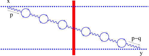
Figure 8: Bubble chain without the quark loop intersection with the shock wave .

or we may have one of the loops in the shock-wave background. (see Fig. 9)

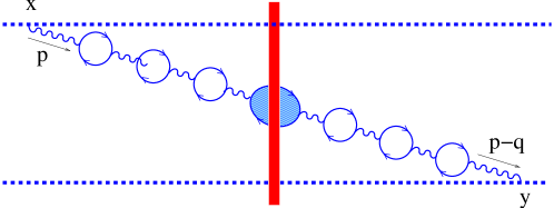
Figure 9: Bubble chain with quark loop crossing the shock wave.

It is easy to see that the sum of these diagrams yields

$${d\over d\eta}{\rm Tr}\{U_{x}U^{\dagger}_{y}\}~{}=~{}2\alpha_{s}{\rm Tr}\{t^{a}U_{x}t^{b}U^{\dagger}_{y}\}\int\!{\textstyle d}\lower 0.12915pt\hbox{\kern-3.99994pt${}^{\scriptstyle-}$}\kern-0.80002pt{}^{2}p{\textstyle d}\lower 0.12915pt\hbox{\kern-3.99994pt${}^{\scriptstyle-}$}\kern-0.80002pt{}^{2}q~{}[e^{i(p,x)_{\perp}}-e^{i(p,y)_{\perp}}][e^{-i(p-q,x)_{\perp}}-e^{-i(p-q,y)_{\perp}}]$$

$$\times~{}{1\over p^{2}(1+{\alpha_{s}\over 6\pi}\ln{\mu^{2}\over p^{2}})}\Big{(}1-{\alpha_{s}n_{f}\over 6\pi}\ln{q^{2}\over\mu^{2}}\Big{)}\partial_{\perp}^{2}U^{ab}(q){1\over(p-q)^{2}(1+{\alpha_{s}\over 6\pi}\ln{\mu^{2}\over(p-q)^{2}})}$$ (45)

where we have left only the UV part (29) of the quark loop. (In principle, one should also include the dressing of the UV-finite $1/N_{c}$ term in Eq. (41) by bubble chain, but I think that it is a separate contribution which has nothing to do with the argument of the BK equation). Replacing the quark part of the $\beta$-function $-{\alpha_{s}\over 6\pi}n_{f}\ln{p^{2}\over\mu^{2}}$ by the total contribution ${\alpha_{s}\over 4\pi}b\ln{p^{2}\over\mu^{2}}$ (where $b-{11\over 3N_{c}}-{2\over 3}n_{f}$), we get

$${d\over d\eta}{\rm Tr}\{U_{x}U^{\dagger}_{y}\}~{}=~{}2{\rm Tr}\{t^{a}U_{x}t^{b}U^{\dagger}_{y}\}$$

$$\times\int\!{\textstyle d}\lower 0.12915pt\hbox{\kern-3.99994pt${}^{\scriptstyle-}$}\kern-0.80002pt{}^{2}p{\textstyle d}\lower 0.12915pt\hbox{\kern-3.99994pt${}^{\scriptstyle-}$}\kern-0.80002pt{}^{2}q~{}[e^{i(p,x)_{\perp}}-e^{i(p,y)_{\perp}}][e^{-i(p-q,x)_{\perp}}-e^{-i(p-q,y)_{\perp}}]{\alpha_{s}(p^{2})\over p^{2}}\alpha_{s}^{-1}(q^{2})\partial_{\perp}^{2}U^{ab}(q){\alpha_{s}((p-q)^{2})\over(p-q)^{2}}$$ (46)

To go to the coordinate space, let us expand the coupling constants in Eq. (46) in powers of $\alpha_{s}=\alpha_{s}(\mu^{2})$, i.e. return back to Eq. (45) with ${\alpha_{s}\over 6\pi}n_{f}\rightarrow-b{\alpha_{s}\over 4\pi}$. In the first order we get the UV part of the NLO BK equation (40)

$${d\over d\eta}{\rm Tr}\{U_{x}U^{\dagger}_{y}\}~{}$$ (47)

$$=~{}{\alpha_{s}\over 2\pi^{2}}\!\int\!d^{2}z~{}[{\rm Tr}\{U_{x}U^{\dagger}_{z}\}{\rm Tr}\{U_{z}U^{\dagger}_{y}\}-N_{c}{\rm Tr}\{U_{x}U^{\dagger}_{y}\}]\Big{[}{(x-y)^{2}\over X^{2}Y^{2}}\Big{(}1+b{\alpha_{s}\over 4\pi}\ln(x-y)^{2}\mu^{2}\Big{)}-b{\alpha_{s}\over 4\pi}{X^{2}-Y^{2}\over X^{2}Y^{2}}\ln{X^{2}\over Y^{2}}\Big{]}$$

In this section, we perform the calculations in the leading log approximation

$$\alpha_{s}\ln{p^{2}\over\mu^{2}}\sim 1,\alpha_{s}\ll 1$$ (48)

(hence we omit the constant term ($\sim{5\over 3}$) from the Eq. (40)).

In the second order in the expansion we obtain

$$-2\alpha_{s}\!\int\!{\textstyle d}\lower 0.12915pt\hbox{\kern-3.99994pt${}^{\scriptstyle-}$}\kern-0.80002pt{}^{2}p{\textstyle d}\lower 0.12915pt\hbox{\kern-3.99994pt${}^{\scriptstyle-}$}\kern-0.80002pt{}^{2}q~{}e^{i(p,x)_{\perp}-i(p-q,y)_{\perp}}{1\over p^{2}(1-{b\alpha_{s}\over 4\pi}\ln{\mu^{2}\over p^{2}})}\Big{(}1-{b\alpha_{s}\over 4\pi}\ln{\mu^{2}\over q^{2}}\Big{)}\partial_{\perp}^{2}U^{ab}(q){1\over(p-q)^{2}(1-{b\alpha_{s}\over 4\pi}\ln{\mu^{2}\over(p-q)^{2}})}~{}=$$

$$-{b^{2}\alpha^{2}_{s}\over 8\pi^{2}}(x|{\ln^{2}{\mu^{2}\over p^{2}}\over p^{2}}\partial_{\perp}^{2}U{1\over p^{2}}+{\ln{\mu^{2}\over p^{2}}\over p^{2}}\partial_{\perp}^{2}U{\ln{\mu^{2}\over p^{2}}\over p^{2}}+{1\over p^{2}}\partial_{\perp}^{2}U{\ln^{2}{\mu^{2}\over p^{2}}\over p^{2}}-{\ln{\mu^{2}\over p^{2}}\over p^{2}}\Big{(}\ln{\mu^{2}\over-\partial_{\perp}^{2}}\partial_{\perp}^{2}U\Big{)}{1\over p^{2}}-{1\over p^{2}}\Big{(}\ln{\mu^{2}\over-\partial_{\perp}^{2}}\partial_{\perp}^{2}U\Big{)}{\ln{\mu^{2}\over p^{2}}\over p^{2}}|y)$$

Again, it is convenient to replace $\partial_{\perp}^{2}U_{z}$ by $\partial_{\perp}^{2}\tilde{U}_{z}$ where $\tilde{U}_{z}=U_{z}-{U_{x}\over 2}-{U_{y}\over 2}$:

Using the formulas

$$(x|-\ln^{2}{\mu^{2}\over p^{2}}\tilde{U}{1\over p^{2}}-{1\over p^{2}}\tilde{U}\ln^{2}{\mu^{2}\over p^{2}}+\ln{\mu^{2}\over p^{2}}\Big{(}\ln{\mu^{2}\over-\partial_{\perp}^{2}}\tilde{U}\Big{)}{1\over p^{2}}+{1\over p^{2}}\Big{(}\ln{\mu^{2}\over-\partial_{\perp}^{2}}\tilde{U}\Big{)}\ln{\mu^{2}\over p^{2}}$$

$$-~{}\ln{\mu^{2}\over p^{2}}\tilde{U}{\ln{\mu^{2}\over p^{2}}\over p^{2}}-{\ln{\mu^{2}\over p^{2}}\over p^{2}}\tilde{U}\ln{\mu^{2}\over p^{2}}|y)+(x|{\ln{\mu^{2}\over p^{2}}\over p^{2}}|y)\Big{[}\Big{(}\ln{\mu^{2}\over-\partial_{\perp}^{2}}\tilde{U}\Big{)}_{x}+\Big{(}\ln{\mu^{2}\over-\partial_{\perp}^{2}}\tilde{U}\Big{)}_{y}\Big{]}$$

$$=\int\!dz~{}\Big{\{}{1\over 4\pi^{2}X^{2}}\Big{[}\ln X^{2}\mu^{2}\ln Y^{2}\mu^{2}-\ln{X^{2}\over Y^{2}}\ln\Delta^{2}\mu^{2}-\ln^{2}\Delta^{2}\mu^{2}\Big{]}$$

$$+~{}{1\over 4\pi^{2}Y^{2}}\Big{[}\ln X^{2}\mu^{2}\ln Y^{2}\mu^{2}+\ln{X^{2}\over Y^{2}}\ln\Delta^{2}\mu^{2}-\ln^{2}\Delta^{2}\mu^{2}\Big{]}\Big{\}}(U_{z}-{1\over 2}U_{x}-{1\over 2}U_{y})$$

and

$$(x|2{p_{i}\ln^{2}{\mu^{2}\over p^{2}}\over p^{2}}\tilde{U}{p_{i}\over p^{2}}+2{p_{i}\ln{\mu^{2}\over p^{2}}\over p^{2}}\tilde{U}{p_{i}\ln{\mu^{2}\over p^{2}}\over p^{2}}+2{p_{i}\over p^{2}}\tilde{U}{p_{i}\ln^{2}{\mu^{2}\over p^{2}}\over p^{2}}-2{p_{i}\ln{\mu^{2}\over p^{2}}\over p^{2}}\Big{(}\ln{\mu^{2}\over-\partial_{\perp}^{2}}U\Big{)}{p_{i}\over p^{2}}$$

$$-~{}2{p_{i}\over p^{2}}\Big{(}\ln{\mu^{2}\over-\partial_{\perp}^{2}}U\Big{)}{p_{i}\ln{\mu^{2}\over p^{2}}\over p^{2}}|y)=~{}\int\!{dz\over 4\pi^{2}}~{}(U_{z}-{1\over 2}U_{x}-{1\over 2}U_{y})\Bigg{\{}\Big{[}{1\over X^{2}}+{1\over Y^{2}}\Big{]}\ln^{2}\Delta^{2}\mu^{2}$$

$$+~{}{\Delta^{2}\over X^{2}Y^{2}}\Bigg{[}-\ln^{2}\Delta^{2}\mu^{2}+{2\Delta_{i}\over\pi\Delta^{2}}\int\!dr~{}\Big{[}{r_{i}Y^{2}-(Y,r)Y_{i}\over r^{2}(Y-r)^{2}}\ln(r-X)^{2}-{r_{i}X^{2}-(X,r)X_{i}\over r^{2}(X-r)^{2}}\ln(r-Y)^{2}\Big{]}\Bigg{]}\Bigg{\}}$$ (49)

we obtain

$${d\over d\eta}{\rm Tr}\{U_{x}U^{\dagger}_{y}\}^{(2)}~{}=~{}{\alpha_{s}\over 2\pi^{2}}\Big{(}{b\alpha_{s}\over 4\pi}\Big{)}^{2}\!\int\!d^{2}z~{}[{\rm Tr}\{U_{x}U^{\dagger}_{z}\}{\rm Tr}\{U_{z}U^{\dagger}_{y}\}-N_{c}{\rm Tr}\{U_{x}U^{\dagger}_{y}\}]$$ (50)

$$\times~{}\Big{[}{(x-y)^{2}\over X^{2}Y^{2}}\ln^{2}(x-y)^{2}\mu^{2}+{1\over X^{2}}\ln{X^{2}\over Y^{2}}(\ln X^{2}\mu^{2}+\ln(x-y)^{2}\mu^{2})-{1\over Y^{2}}\ln{X^{2}\over Y^{2}}(\ln Y^{2}\mu^{2}+\ln(x-y)^{2}\mu^{2})\Big{]}$$

We have omitted the contribution of the last integral in r.h.s. of Eq. (49) since it is negligible in the limits $X\gg Y$, $Y\gg X$ and $X,Y\gg x-y$, and therefore can be dropped in the leading log approximation (48). Adding the first-order contribution (first line in the Eq. (40), we get

$${d\over d\eta}{\rm Tr}\{U_{x}U^{\dagger}_{y}\}~{}=~{}{\alpha_{s}\over 2\pi^{2}}\!\int\!d^{2}z~{}[{\rm Tr}\{U_{x}U^{\dagger}_{z}\}{\rm Tr}\{U_{z}U^{\dagger}_{y}\}-N_{c}{\rm Tr}\{U_{x}U^{\dagger}_{y}\}]\Big{\{}{(x-y)^{2}\over X^{2}Y^{2}}\Big{[}1+{b\alpha_{s}\over 4\pi}\ln(x-y)^{2}\mu^{2}$$

$$+~{}\Big{(}{b\alpha_{s}\over 4\pi}\Big{)}^{2}\ln^{2}(x-y)^{2}\mu^{2}\Big{]}+{b\alpha_{s}\over 4\pi}{1\over X^{2}}\ln{X^{2}\over Y^{2}}\Big{[}1+{b\alpha_{s}\over 4\pi}\ln(x-y)^{2}\mu^{2}+{b\alpha_{s}\over 4\pi}\ln X^{2}\mu^{2}\Big{]}\Big{]}$$

$$-~{}{b\alpha_{s}\over 4\pi}{1\over Y^{2}}\ln{X^{2}\over Y^{2}}\Big{[}1+{b\alpha_{s}\over 4\pi}\ln(x-y)^{2}\mu^{2}+{b\alpha_{s}\over 4\pi}\ln Y^{2}\mu^{2}\Big{]}\Big{\}}$$ (51)

Our guess for the argument of the coupling constant in all orders in $\ln p^{2}/\mu^{2}$ is

$${d\over d\eta}{\rm Tr}\{U_{x}U^{\dagger}_{y}\}~{}=~{}{\alpha_{s}((x-y)^{2})\over 2\pi^{2}}\!\int\!d^{2}z~{}[{\rm Tr}\{U_{x}U^{\dagger}_{z}\}{\rm Tr}\{U_{z}U^{\dagger}_{y}\}-N_{c}{\rm Tr}\{U_{x}U^{\dagger}_{y}\}]$$ (52)

$$\times~{}\Big{[}{(x-y)^{2}\over X^{2}Y^{2}}+{1\over X^{2}}\Big{(}{\alpha_{s}(X^{2})\over\alpha_{s}(Y^{2})}-1\Big{)}+{1\over Y^{2}}\Big{(}{\alpha_{s}(Y^{2})\over\alpha_{s}(X^{2})}-1\Big{)}\Big{]}$$

We see now that the argument of the coupling constant in the BK equation is size of the original dipole $(x-y)^{2}$ as it was advertised in Eq. (5).

V Conclusions and Outlook

First, there are no new operators at the one-loop level - just as at the tree level, the high-energy scattering can be described in terms of Wilson lines. The fact that there are no new operators at the one - loop level is rather remarkable. In the case of the usual light-cone operator expansion this is not true - for example, if we have the operator

$$[GG]=\int\!dudv~{}\theta(u-v)~{}[\infty p_{1},up_{1}]_{x}G_{\bullet i}(up_{1}+x_{\perp})[up_{1},vp_{1}]_{x}G_{\bullet}^{~{}i}(vp_{1}+x_{\perp})[vp_{1},-\infty p_{1}]_{x}$$ (53)

in the leading order, one should expect the operator

$$\alpha_{s}\int\!dudv~{}\theta(u-v)\ln(u-v)~{}[\infty p_{1},up_{1}]_{x}G_{\bullet i}(up_{1}+x_{\perp})[up_{1},vp_{1}]_{x}G_{\bullet}^{~{}i}(vp_{1}+x_{\perp})[vp_{1},-\infty p_{1}]_{x}$$ (54)

in the NLO (in general, any new loop brings an additional factor $\alpha_{s}\ln(u-v)$). This does not happen here, and in addition the operator $[GG]$ appears only in the combination $-i[DG]+[GG]=\partial_{\perp}^{2}U$, exactly as at the tree level. I have checked this by the explicit calculation of the quark-loop contribution and expect to confirm it by the calculation of the gluon loop.

Second conclusion of the paper is that the argument of the coupling constant in the BK equation (obtained from the renormalon-based arguments) appears to be the size of the parent dipole rather than the size of produced dipoles. I have obtained the result for the argument of the coupling constant in the non-linear evolution of dipoles using the quark part of the $\beta$-function. It is necessary to confirm this result by calculating the diagrams with gluon loops. Also, it would be extremely interesting to check how (and if) this argument of the coupling constant arises from the correlation function of the original dipole and the “diamond” high-energy effective actiondiamond formulated in terms of the (renorm-invariant) Wilson lines. The study is in progress.

VI Appendix: Light-cone expansion of the quark-loop contribution to gluon propagator in the background field

The expression (22) should be compared to the light-cone expansion of the quark-loop part of the gluon propagator in an external field. The quark-loop contribution to the propagator of a gluon in the external field has the form:

$$A^{m}_{\bullet}(x)A^{n}_{\bullet}(y)=\!\int\!\!dx^{\prime}dy^{\prime}~{}(x|{1\over P^{2}g_{\bullet\mu}+2iG_{\bullet\mu}+{\cal O}_{\bullet\mu}}|x^{\prime})^{ma}{\rm Tr}\{t^{a}\gamma_{\mu}(x^{\prime}|{1\over\not\!P}|y^{\prime})t^{b}\gamma_{\nu}(y^{\prime}|{1\over\not\!P}|x^{\prime})\}(y^{\prime}|{1\over P^{2}g_{\nu\bullet}+2iG_{\nu\bullet}+{\cal O}_{\nu\bullet}}|y)^{bn}$$ (55)

where

$${\cal O}_{\mu\bullet}={\cal O}_{\bullet\mu}~{}=~{}{1\over\alpha}D^{i}G_{i\mu}={2p_{2\mu}\over\alpha s}D^{i}G_{i\bullet}$$ (56)

An additional term in the gluon propagator is due to the fact that the external gluon field of the target satisfies the Yang-Mills equation with a source $D^{\mu}G^{a}_{\mu\nu}~{}=~{}-g\bar{\psi}\gamma_{\nu}t^{a}\psi$. From the viewpoint of Feynman diagrams in the bF gauge, this term comes from the diagrams with the quark insertions shown in Fig. 10 (in the light-like gauge this term arises automatically, see Ref. npb96, ).

Figure 10: “Target” contribution to the gluon propagator in the external field .

For the contribution $\sim{\cal O}_{\mu\bullet}$ the quark propagator reduces to

$$\gamma_{\mu}t^{a}{(\beta_{p}+\beta_{k})\!\not\!p_{2}+(\not\!p+\not\!k)_{\perp}\over(\alpha_{p}+\alpha_{k})(\beta_{p}+\beta_{k})s-(p+k)_{\perp}^{2}}t^{b}\!\!\not\!p_{1}-t^{b}\!\!\not\!p_{1}{(\beta_{p}-\beta_{k})\!\not\!p_{2}+(\not\!p-\not\!k)_{\perp}\over(\alpha_{p}-\alpha_{k})(\beta_{p}-\beta_{k})s-(p-k)_{\perp}^{2}}t^{a}\gamma_{\mu}$$ (57)

As explained in Ref. mobzor, at $\alpha_{k}\ll\alpha_{p}$ one can shift the contour of integration over $\beta_{p}$ away from the pole in the denominators in the above equation. After that $\beta_{p}\sim{p_{\perp}^{2}\over\alpha_{p}s}$ so one can neglect the terms proportional to transverse momenta in the denominator and in the numerator. One obtains

$${1\over\alpha s}\gamma_{\mu}\!\not\!p_{2}\!\not\!p_{1}t^{a}t^{b}-t^{b}t^{a}\!\!\not\!p_{1}\!\not\!p_{2}\gamma_{\mu}~{}\simeq~{}{1\over\alpha}if^{abc}t^{c}\gamma_{\mu}$$ (58)

which corresponds to the vertex of the insertion of ${\cal O}_{\mu\bullet}$ operator.

We need to expand the Eq. (55) near the near the light cone $x\rightarrow y$ and compare it to the light-cone expansion of the same propagator in the shock-wave background (refvesvkladlikone). The technique for the light-cone expansion of propagators in external fields was developed in Refs. pl83, ; eveq, ). The expansion of the tree-level quark propagator has the formeveq :

$$(x^{\prime}|{1\over\not\!{P}}|y^{\prime})~{}=~{}{\not\!\!\Delta\Gamma(2-\epsilon)\over 2\pi^{2}(-\Delta^{2})^{2-\epsilon}}+{\Gamma(1-\epsilon)\over 16\pi^{2}(-\Delta^{2})^{1-\epsilon}}\!\int_{0}^{1}\!du~{}\Big{\{}\bar{u}\not\!\!\Delta\sigma G(x_{u})+u\sigma G(x_{u})\not\!\!\Delta-2i\bar{u}u\not\!\!\Delta D^{\lambda}G_{\lambda\Delta}$$

$$+~{}4\not\!\!\Delta\!\int_{0}^{u}\!dv~{}\bar{u}vG_{\Delta}^{~{}\xi}(x_{u})G_{\Delta\xi}(x_{v})\Big{\}}$$

$$+~{}{\Gamma(-\epsilon)\over 16\pi^{2}(-\Delta^{2})^{-\epsilon}}\!\int_{0}^{1}\!du~{}\Big{\{}i({1\over 2}-\bar{u}u)D^{\lambda}G_{\lambda\rho}\gamma^{\rho}+{i\over 2}\bar{u}u(1-2u)\hat{D}D^{\lambda}G_{\lambda\Delta}-\bar{u}u(1-2u)\gamma^{\rho}[G_{\Delta}^{~{}\xi}(x_{u}),G_{\rho\xi}(x_{u})]$$

$$-~{}{1\over 2}\bar{u}u\epsilon_{\Delta\mu\nu\lambda}D^{\mu}D_{\xi}G^{\xi\nu}\gamma^{\lambda}\gamma_{5}+i{\bar{u}u\over 2}([G_{\Delta\xi}(x_{u}),\tilde{G}_{\nu}^{~{}\xi}(x_{u})]+[\tilde{G}_{\Delta\xi}(x_{u}),G_{\nu}^{~{}\xi}(x_{u})])\gamma_{\nu}\gamma_{5}$$

$$+\int_{0}^{u}\!dv~{}\Big{[}(\bar{u}-2\bar{u}v-{1\over 2})G_{\Delta\xi}(x_{u})G^{\lambda\xi}(x_{v})\gamma_{\lambda}+(v-2\bar{u}v-{1\over 2})G^{\lambda\xi}(x_{u})G_{\Delta\xi}(x_{v})\gamma_{\lambda}$$

$$+~{}{i\over 2}(1-2\bar{u}-2v)G_{\Delta\xi}(x_{u})\tilde{G}^{\lambda\xi}(x_{v})\gamma_{\lambda}\gamma_{5}-{i\over 2}\tilde{G}_{\Delta\xi}(x_{u})G^{\lambda\xi}(x_{v})\gamma_{\lambda}\gamma_{5}\Big{]}\Big{\}}+O({\rm twist~{}3})$$ (59)

where $\Delta=x^{\prime}-y^{\prime}$ and $\epsilon=1-{d_{\perp}\over 2}$. Hereafter, we use the notations $x_{u}\equiv ux^{\prime}+\bar{u}y^{\prime}$ and $G_{\Delta\mu}\equiv G_{\alpha\mu}\Delta^{\alpha}$ for brevity.

We need to multiply this by similar expansion for the antiquark propagator. The product of the two quark propagators has the form:

$${\rm Tr}~{}t^{a}\gamma^{\alpha}(x^{\prime}|{1\over\!\not\!P}|y^{\prime})t^{b}\gamma^{\beta}(y^{\prime}|{1\over\!\not\!P}|x^{\prime})~{}=~{}(\tilde{T}_{1})_{\alpha\beta}^{ab}+(\tilde{T}_{2})_{\alpha\beta}^{ab}+(\tilde{T}_{3})_{\alpha\beta}^{ab}$$ (60)

where

$$(\tilde{T}_{1})_{\alpha\beta}^{ab}~{}=~{}i{B(2-\epsilon,2-\epsilon)\over 4\pi^{2}}[x^{\prime},y^{\prime}]^{ab}(x^{\prime}|(p^{2}g_{\alpha\beta}-p_{\alpha}p_{\beta}){\Gamma(\epsilon)\over(-p^{2})^{\epsilon}}|y^{\prime})~{}$$

$$+~{}{B(2-\epsilon,1-\epsilon)\over 8\pi^{4}}{\Gamma(3-2\epsilon)\over(-\Delta^{2})^{3-2\epsilon}}\!\int_{0}^{1}\!du~{}\Big{(}[x^{\prime},x_{u}](2i\bar{u}\Delta_{\alpha}G_{\beta\Delta}(x_{u})-2iu\Delta_{\beta}G_{\alpha\Delta}(x_{u})+i\Delta^{2}G_{\alpha\beta}(x_{u}))[x_{u},y^{\prime}]\Big{)}^{ab}$$

(61)

$$(\tilde{T}_{2})_{\alpha\beta}^{ab}~{}=~{}i{B(2-\epsilon,1-\epsilon)\over 8\pi^{4}}{\Gamma(3-2\epsilon)\over(-\Delta^{2})^{3-2\epsilon}}\!\int_{0}^{1}\!du~{}\bar{u}u(2\Delta_{\alpha}\Delta_{\beta}-\Delta^{2}g_{\alpha\beta})\Big{(}[x^{\prime},x_{u}]D^{\lambda}G_{\lambda\Delta})(x_{u})[x_{u},y^{\prime}]\Big{)}^{ab}$$

$$+~{}{B(2-\epsilon,-\epsilon)\over 16\pi^{4}}{\Gamma(2-2\epsilon)\over(\Delta^{2})^{2-2\epsilon}}\!\int_{0}^{1}\!du\Big{(}[x^{\prime},x_{u}][\{[-i({1\over 2}-\bar{u}u)D^{\lambda}G_{\lambda\alpha}(x_{u})\Delta_{\beta}-~{}{i\over 2}\bar{u}u(1-2u)D_{\alpha}D^{\lambda}G_{\lambda\Delta}(x_{u})\Delta_{\beta}+\alpha\leftrightarrow\beta]$$

$$+~{}i({1\over 2}-\bar{u}u)g_{\alpha\beta}D^{\lambda}G_{\lambda\Delta}(x_{u})+~{}{i\over 2}\bar{u}u(1-2u)g_{\alpha\beta}(\Delta\cdot D)D^{\lambda}G_{\lambda\Delta}(x_{u})\}[x_{u},y^{\prime}]\Big{)}^{ab}$$ (62)

$$(\tilde{T}_{3})_{\alpha\beta}^{ab}~{}=-~{}(2\Delta_{\alpha}\Delta_{\beta}-\Delta^{2}g_{\alpha\beta}){B(2-\epsilon,1-\epsilon)\over 2\pi^{4}}{\Gamma(3-2\epsilon)\over(-\Delta^{2})^{3-2\epsilon}}\!\int_{0}^{1}\!dudv~{}{\rm Tr}\Big{\{}\bar{u}v\theta(u-v)t^{b}[y^{\prime},x^{\prime}]t^{a}[x^{\prime},x_{u}]$$

$$\times~{}G_{\Delta\xi}(x_{u})[x_{u},x_{v}]G_{\Delta}^{~{}\xi}(x_{v})[x_{v},y^{\prime}]+u\bar{v}\theta(v-u)t^{a}[x^{\prime},y^{\prime}]t^{b}[y^{\prime},x_{u}]G_{\Delta\xi}(x_{u})[x_{u},x_{v}]G_{\Delta}^{~{}\xi}(x_{v})[x_{v},x^{\prime}]\Big{\}}$$

$$+~{}{B(2-\epsilon,-\epsilon)\over 16\pi^{4}}{\Gamma(2-\epsilon)\over(-\Delta^{2})^{2-\epsilon}}\!\int_{0}^{1}\!dudv~{}{\rm Tr}\Big{\{}-2(\Delta_{\alpha}\delta^{\lambda}_{\beta}+\Delta_{\beta}\delta^{\lambda}_{\alpha}-g_{\alpha\beta}\Delta^{\lambda})\Big{(}\theta(u-v)t^{b}[y^{\prime},x^{\prime}]t^{a}[^{\prime}x,x_{u}]$$

$$\times~{}\{(\bar{u}-2\bar{u}v-{1\over 2})G_{\Delta\xi}(x_{u})[x_{u},x_{v}]G_{\lambda}^{~{}\xi}(x_{v})+(v-2\bar{u}v-{1\over 2})G_{\lambda}^{~{}\xi}(x_{u})[x_{u},x_{v}]G_{\Delta\xi}(x_{v})\}[x_{v},y^{\prime}]$$

$$+~{}\theta(v-u)t^{a}[x^{\prime},y^{\prime}]t^{b}[y^{\prime},x_{u}]\{(u-2\bar{v}u-{1\over 2})G_{\Delta\xi}(x_{u})[x_{u},x_{v}]G_{\lambda}^{~{}\xi}(x_{v})+(\bar{v}-2\bar{v}u-{1\over 2})G_{\lambda}^{~{}\xi}(x_{u})[x_{u},x_{v}]G_{\Delta\xi}(x_{v})\}[x_{v},x^{\prime}]\Big{\}}$$

$$-~{}{B(1-\epsilon,1-\epsilon)\over 16\pi^{4}}{\Gamma(2-2\epsilon)\over(\Delta^{2})^{2-2\epsilon}}\!\int_{0}^{1}\!dudv~{}{\rm Tr}\Big{\{}\Delta^{2}t^{a}([x^{\prime},x_{u}]G_{\alpha\xi}(x_{u})[x_{u},y^{\prime}]t^{b}[y^{\prime},x_{v}]G_{\beta}^{~{}\xi}(x_{v})[x_{v},x^{\prime}]+\alpha\leftrightarrow\beta)+2(\bar{u}v+\bar{v}u)$$

$$\times~{}t^{a}\Big{(}g_{\alpha\beta}[x^{\prime},x_{u}]G_{\Delta\xi}(x_{u})[x_{u},y]t^{b}[y^{\prime},x_{v}]G_{\Delta}^{~{}\xi}(x_{v})[x_{v},x]-[x^{\prime},x_{u}](G_{\Delta\alpha}(x_{u})[x_{u},y]t^{b}[y^{\prime},x_{v}]G_{\Delta\beta}x_{(}v)+\alpha\leftrightarrow\beta)[x_{v},x^{\prime}]\Big{)}$$

$$-~{}2\bar{u}\Delta_{\alpha}t^{a}[x^{\prime},x_{u}]G_{\Delta\xi}(x_{u})[x_{u},y^{\prime}]t^{b}[y^{\prime},x_{v}]G_{\beta}^{~{}\xi}(x_{v})[x_{v},x^{\prime}]-2\bar{v}\Delta_{\alpha}t^{a}[x^{\prime},x_{u}]G_{\beta\xi}(x_{u})[x_{u},y^{\prime}]t^{b}[y^{\prime},x_{v}]G_{\Delta}^{~{}\xi}(v)[x_{v},x^{\prime}]$$

$$-~{}2u\Delta_{\beta}t^{a}[x^{\prime},x_{u}]G_{\Delta\xi}(x_{u})[x_{u},y^{\prime}]t^{b}[y^{\prime},x_{v}]G_{\alpha}^{~{}\xi}(x_{v})[x_{v},x^{\prime}]-2v\Delta_{\beta}t^{a}[x^{\prime},x_{u}]G_{\alpha\xi}(x_{u})[x_{u},y^{\prime}]t^{b}[y^{\prime},x_{v}]G_{\Delta}^{~{}\xi}(x_{v})[x_{v},x^{\prime}]\Big{\}}$$ (63)

where we have omitted terms $\sim\epsilon_{\alpha\beta\mu\nu}\Delta^{\mu}(...)^{\nu}$ and $[G_{\Delta\xi},G_{\nu}^{~{}\xi}]$ which do not contribute to Eq. (55) with our accuracy.

Next we need to substitute the product (67) into the expression (55). Since we will integrate the expression (55) over $x_{\ast}$ and $y_{\ast}$ (to get $U_{x}U^{\dagger}_{y}$) we can neglect the terms proportional to $P_{\alpha}(...)_{\beta}$ and $(...)_{\alpha}P_{\beta}$. Indeed, using the identity

$$P_{\alpha}{1\over P^{2}g_{\alpha\beta}+2iG_{\alpha\beta}}={1\over P^{2}}P_{\beta}+{1\over P^{2}}D^{\mu}G_{\mu\alpha}{1\over P^{2}g_{\alpha\beta}+2iG_{\alpha\beta}}$$ (64)

we get

$$P_{\alpha}{1\over P^{2}g_{\alpha\bullet}+2iG_{\alpha\bullet}+{\cal O}_{\alpha\bullet}}={1\over P^{2}}P_{\bullet},~{}~{}~{}~{}{1\over P^{2}g_{\bullet\alpha}+2iG_{\bullet\alpha}+{\cal O}_{\bullet\alpha}}P_{\alpha}=P_{\bullet}{1\over P^{2}}$$ (65)

As explained in Ref. mobzor, , one can drop the terms proportional to $P_{\bullet}$ since they lead to the terms proportional to the integral of total derivative, namely

$$\int dx_{\ast}[\infty p_{1},{2\over s}x_{\ast}p_{1}]t^{a}[{2\over s}x_{\ast}p_{1},-\infty p_{1}](D_{\bullet}\Phi({2\over s}x_{\ast}p_{1},...))_{ab}$$ (66)

$$= \int dx_{\ast}\frac{d}{dx_{\ast}}\{[\infty p_{1},{2\over s}x_{\ast}p_{1}]t^{a}[{2\over s}x_{\ast}p_{1},-\infty p_{1}](\Phi({2\over s}x_{\ast}p_{1},...))_{ab}\}=0$$

Using this property one can rewrite Eq. (67) in the form

$${\rm Tr}~{}t^{a}\gamma^{\alpha}(x^{\prime}|{1\over\!\not\!P}|y^{\prime})t^{b}\gamma^{\beta}(y^{\prime}|{1\over\!\not\!P}|x^{\prime})~{}\Leftrightarrow~{}(T_{1})_{\alpha\beta}^{ab}+(T_{2})_{\alpha\beta}^{ab}+(T_{3})_{\alpha\beta}^{ab}$$ (67)

where

$$(T_{1})_{\alpha\beta}^{ab} = ig_{\alpha\beta}{\Gamma^{2}(2-\epsilon)\over 4\pi^{2}\Gamma(4-2\epsilon)}(x|P^{2}{\Gamma(\epsilon)\over(-P^{2})^{\epsilon}}|y)^{ab}-{g\Gamma^{2}(2-\epsilon)\over 4\pi^{4}\Gamma(3-2\epsilon)}(x|{\Gamma(\epsilon)\over(-p^{2})^{\epsilon}}|y)\!\!\int_{0}^{1}\!\!du~{}([x^{\prime},x_{u}]G_{\alpha\beta}(x_{u})[x_{u},y^{\prime}])^{ab}$$

$$+ {ig\over 8\pi^{2}}{\Gamma(3-\epsilon)\Gamma(1-\epsilon)\over\Gamma(4-2\epsilon)}(x|{\Gamma(\epsilon)p_{\rho}\over(-p^{2})^{\epsilon}}|y)\!\!\int_{0}^{1}\!\!du~{}([x^{\prime},x_{u}][\bar{u}\delta^{\rho}_{\alpha}G_{\Delta\beta}(x_{u})-u\delta^{\rho}_{\beta}G_{\Delta\alpha}(x_{u})][x_{u},y^{\prime}])^{ab}$$

$$(T_{2})_{\alpha\beta}^{ab} = g_{\alpha\beta}(1-2\epsilon){g\Gamma^{2}(2-\epsilon)\over 4\pi^{2}\Gamma(4-2\epsilon)}(x|{\Gamma(1+\epsilon)\over(-p^{2})^{1+\epsilon}}|y)\!\int_{0}^{1}\!\!du~{}([x^{\prime},x_{u}]D^{\mu}G^{ab}_{\mu\Delta}(x_{u})[x_{u},y^{\prime}])^{ab}+(\tilde{T}_{2})_{\alpha\beta}^{ab}$$ (68)

$$(T_{3})_{\alpha\beta}^{ab} = ig_{\alpha\beta}(1-2\epsilon){g^{2}\Gamma^{2}(2-\epsilon)\over 2\pi^{2}\Gamma(4-2\epsilon)}(x|{\Gamma(1+\epsilon)\over(-p^{2})^{1+\epsilon}}|y)\!\int_{0}^{1}\!\!du\!\!\int_{0}^{u}\!\!\!dv~{}\bar{u}v([x^{\prime},x_{u}]G_{\Delta\xi}(x_{u})[x_{u},x_{v}]G_{\Delta}^{~{}\xi}(x_{v})[x_{v},y^{\prime}])^{ab}+(\tilde{T}_{3})_{\alpha\beta}^{ab}$$

and $\Leftrightarrow$ means “equal up to the contributions $\sim~{}P_{\alpha}(...)_{\beta}$ and $(...)_{\alpha}P_{\beta}$”.

Next we expand the propagator (55) near the light cone. The first contribution comes from the $T_{1}$ term which represents diagrams in Fig. 11 a-g.

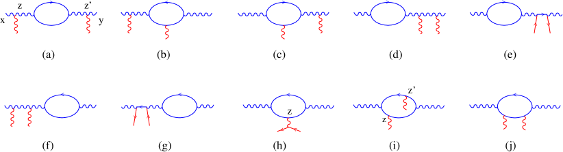
Figure 11: Quark-loop contribution to the gluon propagator in an external field .

The calculation yields

$$\!\int\!\!dx^{\prime}dy^{\prime}~{}(x|{1\over P^{2}g_{\bullet\mu}+2iG_{\bullet\mu}+{\cal O}_{\bullet\mu}}|x^{\prime})^{ma}T_{1\alpha\beta}^{ab}(y^{\prime}|{1\over P^{2}g_{\nu\bullet}+2iG_{\nu\bullet}+{\cal O}_{\nu\bullet}}|y)^{bn}$$

$$=~{}{1\over 8\pi^{2}}B(2-\epsilon,2-\epsilon)(x|{1\over p^{2}}\Big{\{}{\partial_{\perp}^{2}U^{ab}\over\alpha},{\Gamma(\epsilon)\over(-p^{2})^{\epsilon}}\Big{\}}{1\over p^{2}}|y)-{ig\over 4\pi^{2}}B(2-\epsilon,2-\epsilon)(x|{1\over p^{2}}\Big{\{}{D^{i}G_{i{\bullet}}^{ab}\over\alpha},{\Gamma(\epsilon)\over(-p^{2})^{\epsilon}}\Big{\}}{1\over p^{2}}|y)$$

$$+~{}{g^{2}\Gamma^{2}(1-\epsilon)\over 32\pi^{2}\Gamma(4-2\epsilon)}\!\int_{0}^{\infty}\!{{\textstyle d}\lower 0.12915pt\hbox{\kern-3.99994pt${}^{\scriptstyle-}$}\kern-0.80002pt{}\alpha\over\alpha^{3}}\!\int_{y_{\ast}}^{x_{\ast}}\!\!d{2\over s}z_{\ast}\!\int_{y_{\ast}}^{z_{\ast}}\!\!d{2\over s}z^{\prime}_{\ast}~{}([x_{\ast},z_{\ast}]_{x}G_{{\bullet}i}(z_{\ast},x_{\perp})[z_{\ast},z^{\prime}_{\ast}]_{x}G_{{\bullet}j}(z^{\prime}_{\ast},x_{\perp})[z^{\prime}_{\ast},y_{\ast}]_{x})^{ab}$$

$$\times~{}\Big{(}{4i\over\alpha s}\Big{)}^{\epsilon}\Bigg{\{}g_{ij}\Big{[}{1\over\epsilon}[(2-\epsilon)(x-z^{\prime})_{\ast}^{\epsilon}-(x-z)_{\ast}^{\epsilon}-(z-z^{\prime})_{\ast}^{\epsilon}]+{1\over\epsilon}[(2-\epsilon)(z-y)_{\ast}^{\epsilon}-(z^{\prime}-y)_{\ast}^{\epsilon}-(z-z^{\prime})_{\ast}^{\epsilon}]$$

$$+~{}2(z-z^{\prime})_{\ast}^{\epsilon}-2(2-\epsilon){(z-z^{\prime})_{\ast}\over(x-z^{\prime})_{\ast}^{1-\epsilon}}+(1-\epsilon){(z-z^{\prime})_{\ast}^{2}\over(x-z^{\prime})_{\ast}^{2-\epsilon}}-2(2-\epsilon){(z-z^{\prime})_{\ast}\over(z-y)_{\ast}^{1-\epsilon}}+(1-\epsilon){(z-z^{\prime})_{\ast}^{2}\over(z-i)_{\ast}^{2-\epsilon}}$$

$$+~{}{2(1-\epsilon)\over 3-\epsilon}(z-z^{\prime})_{\ast}^{2}[\Delta_{\ast}^{-2+\epsilon}+(z-z^{\prime})_{\ast}^{-2+\epsilon}-(x-z)_{\ast}^{-2+\epsilon}-(z^{\prime}-y)_{\ast}^{-2+\epsilon}]\Big{]}$$

$$+~{}{1\over(1+\epsilon)}\Big{[}(x-z)_{\ast}^{1+\epsilon}+(z-z^{\prime})_{\ast}^{1+\epsilon}-(x-z^{\prime})_{\ast}^{1+\epsilon}+(1+\epsilon){(x-z)_{\ast}(z-z^{\prime})_{\ast}\over(x-z^{\prime})_{\ast}^{1-\epsilon}}+(z^{\prime}-y)_{\ast}^{1+\epsilon}+(z-z^{\prime})_{\ast}^{1+\epsilon}$$

$$-~{}(z-y)_{\ast}^{1+\epsilon}+(1+\epsilon){(z-z^{\prime})_{\ast}(z^{\prime}-i)_{\ast}\over(x-z^{\prime})_{\ast}^{1-\epsilon}}\Big{]}\Big{(}{(3-\epsilon)g_{ij}\over\Delta_{\ast}}+i{\alpha s\over 4\Delta_{\ast}^{2}}[\Delta_{\perp}^{2}g_{ij}-\Delta_{i}\Delta_{j}]\Big{)}$$

$$+~{}{g_{ij}\over\epsilon}(1-\epsilon)(3-2\epsilon)[2(z-z^{\prime})_{\ast}^{\epsilon}+(x-z)_{\ast}^{\epsilon}+(z-y)_{\ast}^{\epsilon}-2(x-z^{\prime})_{\ast}^{\epsilon}-2(z^{\prime}-y)_{\ast}^{\epsilon}]\Bigg{\}}~{}\Big{(}-{i\alpha s\over 4\pi\Delta_{\ast}}\Big{)}^{1-\epsilon}e^{i{\Delta_{\perp}^{2}\over 4\Delta_{\ast}}\alpha s}$$ (69)

In our “external” field the characteristic distances $z_{\ast}(z^{\prime}_{\ast})$ are of the order of width of the shock wave: $z_{\ast},z^{\prime}_{\ast}\sim e^{\eta_{2}}\sqrt{s/m^{2}}$. As we shall see below, the characteristic distances $x_{\ast}$ and $y_{\ast}$ are $\sim e^{\eta_{2}}\sqrt{s/m^{2}}$ so we can neglect $z_{\ast}$ and $z^{\prime}_{\ast}$ in comparison to $x_{\ast}$ and/or $y_{\ast}$. The formula (69) simplifies to

$$\!\int\!\!dx^{\prime}dy^{\prime}~{}(x|{1\over P^{2}g_{\bullet\mu}+2iG_{\bullet\mu}+{\cal O}_{\bullet\mu}}|x^{\prime})^{ma}T_{1\alpha\beta}^{ab}(y^{\prime}|{1\over P^{2}g_{\nu\bullet}+2iG_{\nu\bullet}+{\cal O}_{\nu\bullet}}|y)^{bn}$$

$$=~{}{1\over 8\pi^{2}}B(2-\epsilon,2-\epsilon)(x|{1\over p^{2}}\Big{\{}{\partial_{\perp}^{2}U^{ab}\over\alpha},{\Gamma(\epsilon)\over(-p^{2})^{\epsilon}}\Big{\}}{1\over p^{2}}|y)+{ig^{3}\over 16\pi^{2}}{B(2-\epsilon,2-\epsilon)\over\epsilon}\!\int_{0}^{\infty}\!{{\textstyle d}\lower 0.12915pt\hbox{\kern-3.99994pt${}^{\scriptstyle-}$}\kern-0.80002pt{}\alpha\over\alpha^{3}}$$

$$\times~{}\Big{(}{4i\over\alpha s}\Big{)}^{\epsilon}[x_{\ast}^{\epsilon}+(-y)_{\ast}^{\epsilon}]~{}\Big{(}-{i\alpha s\over 4\pi\Delta_{\ast}}\Big{)}^{1-\epsilon}e^{i{\Delta_{\perp}^{2}\over 4\Delta_{\ast}}\alpha s}\!\int_{y_{\ast}}^{x_{\ast}}\!\!d{2\over s}z_{\ast}~{}([x_{\ast},z_{\ast}]_{x}D^{i}G_{i{\bullet}}(z_{\ast},x_{\perp})[z_{\ast},z^{\prime}_{\ast}]_{x}[z_{\ast},y_{\ast}]_{x})^{ab}$$

$$+~{}{g^{2}\Gamma(1-\epsilon)\Gamma(2-\epsilon)\over 16\pi^{2}\Gamma(4-2\epsilon)}\!\int_{0}^{\infty}\!{{\textstyle d}\lower 0.12915pt\hbox{\kern-3.99994pt${}^{\scriptstyle-}$}\kern-0.80002pt{}\alpha\over\alpha^{3}}\!\int_{y_{\ast}}^{x_{\ast}}\!\!d{2\over s}z_{\ast}\!\int_{y_{\ast}}^{z_{\ast}}\!\!d{2\over s}z^{\prime}_{\ast}~{}([x_{\ast},z_{\ast}]_{x}G_{\bullet}^{~{}i}(z_{\ast},x_{\perp})[z_{\ast},z^{\prime}_{\ast}]_{x}G_{{\bullet}i}(z^{\prime}_{\ast},x_{\perp})[z^{\prime}_{\ast},y_{\ast}]_{x})^{ab}$$

$$\times~{}\Big{(}{4i\over\alpha s}\Big{)}^{\epsilon}\Big{\{}-{1-\epsilon\over\epsilon}[x_{\ast}^{\epsilon}+(-y)_{\ast}^{\epsilon}-2(z-z^{\prime})_{\ast}^{\epsilon}]+{1\over 3-\epsilon}(z-z^{\prime})_{\ast}^{\epsilon}\Big{\}}~{}\Big{(}-{i\alpha s\over 4\pi\Delta_{\ast}}\Big{)}^{1-\epsilon}e^{i{\Delta_{\perp}^{2}\over 4\Delta_{\ast}}\alpha s}$$ (70)

The term $\sim T_{2}$ coming from the diagram in Fig. 11h has the form

$$\!\int\!\!dx^{\prime}dy^{\prime}~{}(x|{1\over p^{2}}|x^{\prime})T_{2\bullet\bullet}^{ab}(y^{\prime}|{1\over p^{2}}|y)$$ (71)

$$=~{}-{i\over 32\pi^{2}}\!\int_{0}^{\infty}\!{{\textstyle d}\lower 0.12915pt\hbox{\kern-3.99994pt${}^{\scriptstyle-}$}\kern-0.80002pt{}\alpha\over\alpha^{3}}\Big{(}{i\over\alpha s}\Big{)}^{\epsilon}\Big{(}-{i\alpha s\over 4\pi\Delta_{\ast}}\Big{)}^{1-\epsilon}e^{i{\Delta_{\perp}^{2}\over 4\Delta_{\ast}}\alpha s}~{}{\Gamma(2-\epsilon)\Gamma(1-\epsilon)\over\Gamma(3-2\epsilon)}\Bigg{\{}{(4-\epsilon)(1-\epsilon)\over\epsilon(2-\epsilon)(3-\epsilon)}[x_{\ast}^{\epsilon}+(-y)_{\ast}^{\epsilon}-\Delta_{\ast}^{\epsilon}-\epsilon x_{\ast}y_{\ast}\Delta_{\ast}^{\epsilon-2}]$$

$$-~{}{2(2-2\epsilon+\epsilon^{2})\over\epsilon(2-\epsilon)(1-\epsilon^{2})}\Big{[}{1-\epsilon\over\Delta_{\ast}}+{i\alpha s\Delta_{\perp}^{2}\over 4\Delta_{\ast}^{2}}\Big{]}[x_{\ast}^{1+\epsilon}+(-y)_{\ast}^{1+\epsilon}-\Delta_{\ast}^{1+\epsilon}-{(1+\epsilon)x_{\ast}y_{\ast}\over\Delta_{\ast}^{1-\epsilon}}]-{1\over\epsilon(1-\epsilon)(2+\epsilon)}\Big{[}{(2-\epsilon)(1-\epsilon)\over\Delta_{\ast}^{2}}$$

$$+~{}{i(2-\epsilon)\alpha s\over 2\Delta_{\ast}^{3}}\Delta_{\perp}^{2}-{\alpha^{2}s^{2}\over 16\Delta_{\ast}^{4}}\Delta_{\perp}^{4}\Big{]}[x_{\ast}^{2+\epsilon}+(-y)_{\ast}^{2+\epsilon}-\Delta_{\ast}^{2+\epsilon}-(2+\epsilon)x_{\ast}y_{\ast}\Delta_{\ast}^{\epsilon}]\Bigg{\}}\!\int_{y_{\ast}}^{x_{\ast}}\!\!d{2\over s}z_{\ast}([x_{\ast},z_{\ast}]_{x}D^{\lambda}G_{\lambda{\bullet}}(z_{\ast},x_{\perp})[z_{\ast},y_{\ast}]_{x}^{ab}$$

where we have neglected $z_{\ast}$ in comparison to $x_{\ast},y_{\ast}$ as discussed above. Since there is no field outside the shock wave, at $x_{\ast}y_{\ast}>0$ the contribution (71) vanishes and at $x_{\ast}>0,y_{\ast}<0$ one can extend the limits of integration over $z_{\ast}$ to $\pm\infty$ and get

$$\!\int\!\!dx^{\prime}dy^{\prime}~{}(x|{1\over p^{2}}|x^{\prime})T_{2\bullet\bullet}^{ab}(y^{\prime}|{1\over p^{2}}|y)$$ (72)

$$\stackrel{{\scriptstyle x_{\ast}>0>y_{\ast}}}{{=}}~{}-{i\over 32\pi^{2}}\!\int_{0}^{\infty}\!{{\textstyle d}\lower 0.12915pt\hbox{\kern-3.99994pt${}^{\scriptstyle-}$}\kern-0.80002pt{}\alpha\over\alpha^{3}}\Big{(}{i\over\alpha s}\Big{)}^{\epsilon}\Big{(}-{i\alpha s\over 4\pi\Delta_{\ast}}\Big{)}^{1-\epsilon}e^{i{\Delta_{\perp}^{2}\over 4\Delta_{\ast}}\alpha s}~{}{\Gamma(2-\epsilon)\Gamma(1-\epsilon)\over\epsilon\Gamma(3-2\epsilon)}\Big{\{}{(4-\epsilon)(1-\epsilon)\over(2-\epsilon)(3-\epsilon)}[x_{\ast}^{\epsilon}+(-y)_{\ast}^{\epsilon}$$

$$-~{}\Delta_{\ast}^{\epsilon}-\epsilon x_{\ast}y_{\ast}\Delta_{\ast}^{\epsilon-2}]-{2(2-2\epsilon+\epsilon^{2})\over(2-\epsilon)(1-\epsilon^{2})}\Big{[}{1-\epsilon\over\Delta_{\ast}}+{i\alpha s\Delta_{\perp}^{2}\over 4\Delta_{\ast}^{2}}\Big{]}[x_{\ast}^{1+\epsilon}+(-y)_{\ast}^{1+\epsilon}-\Delta_{\ast}^{1+\epsilon}-{(1+\epsilon)x_{\ast}y_{\ast}\over\Delta_{\ast}^{1-\epsilon}}]$$

$$-~{}{1\over(1-\epsilon)(2+\epsilon)}\Big{[}{(2-\epsilon)(1-\epsilon)\over\Delta_{\ast}^{2}}+{i(2-\epsilon)\alpha s\over 2\Delta_{\ast}^{3}}\Delta_{\perp}^{2}-{\alpha^{2}s^{2}\over 16\Delta_{\ast}^{4}}\Delta_{\perp}^{4}\Big{]}[x_{\ast}^{2+\epsilon}+(-y)_{\ast}^{2+\epsilon}-\Delta_{\ast}^{2+\epsilon}-(2+\epsilon)x_{\ast}y_{\ast}\Delta_{\ast}^{\epsilon}]\Big{\}}~{}[DG]_{x}^{ab}$$

where $[DG]$ is defined by Eq. (21). Similarly, the integral $\int_{y_{\ast}}^{x_{\ast}}\!\!d{2\over s}z_{\ast}([x_{\ast},z_{\ast}]_{x}D^{\lambda}G_{\lambda{\bullet}}(z_{\ast},x_{\perp})$ in the second term in the r.h.s. of Eq. (70) can be reduced to $[DG]_{x}$. The case $x_{\ast}<0,y_{\ast}>0$ is obtained from (72) by the substitution $x\leftrightarrow y$.

The contribution of diagrams in Fig. 11 i,j is

$$\!\int\!\!dx^{\prime}dy^{\prime}~{}(x|{1\over p^{2}}|x^{\prime})T_{3\bullet\bullet}^{ab}(y^{\prime}|{1\over p^{2}}|y)$$ (73)

$$=~{}{g^{2}\over 16\pi^{2}}B(1-\epsilon,2-\epsilon)\!\int_{0}^{\infty}\!{{\textstyle d}\lower 0.12915pt\hbox{\kern-3.99994pt${}^{\scriptstyle-}$}\kern-0.80002pt{}\alpha\over\alpha^{3}}\Big{(}{4i\over\alpha s}\Big{)}^{\epsilon}\Big{(}-{i\alpha s\over 4\pi\Delta_{\ast}}\Big{)}^{1-\epsilon}e^{i{\Delta_{\perp}^{2}\over 4\Delta_{\ast}}\alpha s}\!\int_{y_{\ast}}^{x_{\ast}}\!\!d{2\over s}z_{\ast}\!\int_{y_{\ast}}^{z_{\ast}}\!\!d{2\over s}z^{\prime}_{\ast}$$

$$\times~{}\Bigg{(}\Bigg{\{}{(4-\epsilon)(1-\epsilon)\over\epsilon(2-\epsilon)(3-\epsilon)}[x_{\ast}^{\epsilon}+(-y)_{\ast}^{\epsilon}-\Delta_{\ast}^{\epsilon}-(z-z^{\prime})_{\ast}^{\epsilon}]-{(z-z^{\prime})_{\ast}^{\epsilon}\over(2-\epsilon)(3-\epsilon)}-{(4-\epsilon)(1-\epsilon)x_{\ast}y_{\ast}\over(2-\epsilon)(3-\epsilon)\Delta_{\ast}^{2-\epsilon}}$$

$$-~{}\Big{[}{1-\epsilon\over\Delta_{\ast}}+{i\alpha s\Delta_{\perp}^{2}\over 4\Delta_{\ast}^{2}}\Big{]}{2(2-2\epsilon+\epsilon^{2})\over\epsilon(1-\epsilon^{2})(2-\epsilon)}[x_{\ast}^{1+\epsilon}+(-y)_{\ast}^{1+\epsilon}-~{}\Delta_{\ast}^{1+\epsilon}-(1+\epsilon)x_{\ast}y_{\ast}\Delta_{\ast}^{\epsilon-1}]$$

$$-~{}\Big{[}{(2-\epsilon)(1-\epsilon)\over\Delta_{\ast}^{2}}+{i(2-\epsilon)\alpha s\over 2\Delta_{\ast}^{3}}\Delta_{\perp}^{2}-{\alpha^{2}s^{2}\over 16\Delta_{\ast}^{4}}\Delta_{\perp}^{4}\Big{]}{[x_{\ast}^{2+\epsilon}+(-y)_{\ast}^{2+\epsilon}-\Delta_{\ast}^{2+\epsilon}-(2+\epsilon)x_{\ast}y_{\ast}\Delta_{\ast}^{\epsilon}]\over\epsilon(1-\epsilon)(2+\epsilon)}\Bigg{\}}$$

$$\hskip 73.97716pt\times~{}([x_{\ast},z_{\ast}]_{x}G_{{\bullet}i}(z_{\ast},x_{\perp})[z_{\ast},z^{\prime}_{\ast}]_{x}G_{\bullet}^{~{}i}(z^{\prime}_{\ast},x_{\perp})[z^{\prime}_{\ast},y_{\ast}])^{ab}$$

$$+~{}\Bigg{\{}-g_{ij}{x_{\ast}y_{\ast}\over\Delta_{\ast}^{2-\epsilon}}-~{}2\Big{[}{1-\epsilon\over\Delta_{\ast}}+{i\alpha s\Delta_{\perp}^{2}\over 4\Delta_{\ast}^{2}}\Big{]}g_{ij}{2-2\epsilon+\epsilon^{2}\over\epsilon(1-\epsilon^{2})(2-\epsilon)}[x_{\ast}^{1+\epsilon}+(-y)_{\ast}^{1+\epsilon}-\Delta_{\ast}^{1+\epsilon}-(1+\epsilon)x_{\ast}y_{\ast}\Delta_{\ast}^{\epsilon-1}]$$

$$-~{}\Big{[}{(2-\epsilon)(1-\epsilon)\over\Delta_{\ast}^{2}}+{i(2-\epsilon)\alpha s\over 2\Delta_{\ast}^{3}}\Delta_{\perp}^{2}-{\alpha^{2}s^{2}\over 16\Delta_{\ast}^{4}}\Delta_{\perp}^{4}\Big{]}{[x_{\ast}^{2+\epsilon}+(-y)_{\ast}^{2+\epsilon}-\Delta_{\ast}^{2+\epsilon}-(2+\epsilon)x_{\ast}y_{\ast}\Delta_{\ast}^{\epsilon}]\over\epsilon(1-\epsilon)(2+\epsilon)}g_{ij}$$

$$-~{}\Big{[}{1-\epsilon\over\Delta_{\ast}}+{i\alpha s\Delta_{\perp}^{2}\over 4\Delta_{\ast}^{2}}\Big{]}g_{ij}{x_{\ast}^{1+\epsilon}+(-y)_{\ast}^{1+\epsilon}-\Delta_{\ast}^{1+\epsilon}\over\epsilon(1+\epsilon)}-\Big{[}2{g_{ij}\over\Delta_{\ast}}-{i\alpha s\over\Delta_{\ast}^{2}}\Delta_{i}\Delta_{j}\Big{]}{x_{\ast}^{1+\epsilon}+(-y_{\ast})^{1+\epsilon}-\Delta_{\ast}^{1+\epsilon}-(1+\epsilon)x_{\ast}y_{\ast}\Delta_{\ast}^{\epsilon-1}\over(1-\epsilon^{2})(2-\epsilon)}\Bigg{\}}$$

$$\hskip 45.5244pt\times~{}[x_{\ast},z_{\ast}]^{am}2{\rm Tr}\{t^{m}G_{{\bullet}i}(z_{\ast},x_{\perp})[z_{\ast},z^{\prime}_{\ast}]t^{n}G_{{\bullet}j}(z^{\prime}_{\ast},x_{\perp})[z^{\prime}_{\ast},z_{\ast}]_{x}+m\leftrightarrow n\}[z_{\ast},y_{\ast}]_{x}^{nb}\Bigg{)}$$

The final expression for the light-cone expansion of the quark-loop contribution to gluon propagator in the sum of the expressions (70), (71), and (73). A very important observation is that the contributions proportional to

$$g^{4}n_{f}\int\!dz_{\ast}\!\int dz^{\prime}_{\ast}~{}\theta(z-z^{\prime})~{}(z-z^{\prime})^{\epsilon}G_{{\bullet}i}(z_{\ast})G_{{\bullet}i}(z^{\prime}_{\ast})$$ (74)

present in the Eqs. (70) and (73) cancel in their sum. If it were not true, there would be an addtional contribution to the gluon propagator (7) at the $g^{4}$ level coming from the small-size (large-momenta) quark loop. Indeed, the calculations of Feynman diagrams with the propagators (7) and (12) implies that we first take limit $z_{\ast},z^{\prime}_{\ast}\rightarrow 0$ and limit $d_{\perp}\rightarrow 2$ afterwards. With such order of limits, the contribution (74) vanishes. However, the proper order of these limits is to take at first $d_{\perp}\rightarrow 2$ (which will give finite expressions after adding the counterterms) and then try to impose the condition that the external field is very narrow by taking the limit $z_{\ast},z^{\prime}_{\ast}\rightarrow 0$. In this case, Eq. (74) reduces to $g^{4}n_{f}[GG]$. The non-commutativity of these limits would mean that the contribution ${1\over p^{2}}[GG]{1\over p^{2}}$ should be added to the gluon propagator (7) to restore the correct result. Fortunately, the terms $\sim$ (74) cancel which means that there are no additional contributions to the gluon propagator coming from the quark loop inside the shock wave ($\equiv$ quark loop with large momenta).

Since there is no external field outside the shock wave, after cancellation of the terms $\sim(z-z^{\prime})^{\epsilon}$ we see that at $x_{\ast}y_{\ast}>0$ the sum of Eq. (70) and Eq. (73) vanishes, and at $x_{\ast}>0>y_{\ast}$ one can extend the limits of integration in the gluon operators to $\pm\infty$ and obtain

$$\int_{y_{\ast}}^{x_{\ast}}\!\!\!dz_{\ast}\!\int_{y_{\ast}}^{x_{\ast}}\!\!\!dz^{\prime}_{\ast}~{}([x_{\ast},z_{\ast}]_{x}G_{{\bullet}i}(z_{\ast},x_{\perp})[z_{\ast},z^{\prime}_{\ast}]_{x}G_{{\bullet}i}(z^{\prime}_{\ast},x_{\perp})[z^{\prime}_{\ast},y_{\ast}]_{x})^{ab}~{}\rightarrow~{}[GG]^{ab}_{x}$$ (75)

$$\int_{y_{\ast}}^{x_{\ast}}\!\!\!dz_{\ast}\!\int_{y_{\ast}}^{z_{\ast}}\!\!\!dz^{\prime}_{\ast}~{}[x_{\ast},z_{\ast}]^{am}{\rm Tr}\{t^{m}G_{{\bullet}i}(z_{\ast},x_{\perp})[z_{\ast},z^{\prime}_{\ast}]t^{n}G_{{\bullet}j}(z^{\prime}_{\ast},x_{\perp})[z^{\prime}_{\ast},z_{\ast}]_{x}+m\leftrightarrow n\}[z_{\ast},y_{\ast}]_{x}^{nb}~{}\rightarrow~{}{\rm Tr}\{t^{a}\partial_{i}U_{x}t^{b}\partial_{j}U^{\dagger}_{x}\}$$

We get

$$\!\int\!\!dx^{\prime}dy^{\prime}~{}(x|{1\over P^{2}g_{\bullet\alpha}+2iG_{\bullet\alpha}+{\cal O}_{\bullet\alpha}}|x^{\prime})^{ma}(T_{1\alpha\beta}^{ab}+T_{2\alpha\beta}^{ab}+T_{3\alpha\beta}^{ab})(y^{\prime}|{1\over P^{2}g_{\beta\bullet}+2iG_{\beta\bullet}+{\cal O}_{\beta\bullet}}|y)^{bn}$$

$$\stackrel{{\scriptstyle x_{\ast}>0>y_{\ast}}}{{=}}~{}{1\over 8\pi^{2}}B(2-\epsilon,2-\epsilon)(x|{1\over p^{2}}\Big{\{}{\partial_{\perp}^{2}U^{ab}\over\alpha},{\Gamma(\epsilon)\over(-p^{2})^{\epsilon}}\Big{\}}{1\over p^{2}}|y)~{}+~{}{g^{2}\over 32\pi^{2}}B(1-\epsilon,2-\epsilon)\!\int_{0}^{\infty}\!{{\textstyle d}\lower 0.12915pt\hbox{\kern-3.99994pt${}^{\scriptstyle-}$}\kern-0.80002pt{}\alpha\over\alpha^{3}}\Big{(}{4i\over\alpha s}\Big{)}^{\epsilon}$$

$$\times~{}\Big{(}-{i\alpha s\over 4\pi\Delta_{\ast}}\Big{)}^{1-\epsilon}e^{i{\Delta_{\perp}^{2}\over 4\Delta_{\ast}}\alpha s}\Bigg{(}\Bigg{\{}-{1-\epsilon\over\epsilon(3-2\epsilon)}[x_{\ast}^{\epsilon}+(-y)_{\ast}^{\epsilon}]+{(4-\epsilon)(1-\epsilon)\over\epsilon(2-\epsilon)(3-\epsilon)}[x_{\ast}^{\epsilon}+(-y)_{\ast}^{\epsilon}-\Delta_{\ast}^{\epsilon}-\epsilon x_{\ast}y_{\ast}\Delta_{\ast}^{\epsilon-2}]$$

$$-~{}\Big{[}{1-\epsilon\over\Delta_{\ast}}+{i\alpha s\Delta_{\perp}^{2}\over 4\Delta_{\ast}^{2}}\Big{]}{2(2-2\epsilon+\epsilon^{2})\over\epsilon(1-\epsilon^{2})(2-\epsilon)}[x_{\ast}^{1+\epsilon}+(-y)_{\ast}^{1+\epsilon}-~{}\Delta_{\ast}^{1+\epsilon}-(1+\epsilon)x_{\ast}y_{\ast}\Delta_{\ast}^{\epsilon-1}]$$

$$-~{}\Big{[}{(2-\epsilon)(1-\epsilon)\over\Delta_{\ast}^{2}}+{i(2-\epsilon)\alpha s\over 2\Delta_{\ast}^{3}}\Delta_{\perp}^{2}-{\alpha^{2}s^{2}\over 16\Delta_{\ast}^{4}}\Delta_{\perp}^{4}\Big{]}{[x_{\ast}^{2+\epsilon}+(-y)_{\ast}^{2+\epsilon}-\Delta_{\ast}^{2+\epsilon}-(2+\epsilon)x_{\ast}y_{\ast}\Delta_{\ast}^{\epsilon}]\over\epsilon(1-\epsilon)(2+\epsilon)}\Bigg{\}}~{}\partial_{\perp}^{2}U_{x}^{ab}$$

$$+~{}\Bigg{\{}-{x_{\ast}y_{\ast}\over\Delta_{\ast}^{2-\epsilon}}-~{}2\Big{[}{1-\epsilon\over\Delta_{\ast}}+{i\alpha s\Delta_{\perp}^{2}\over 4\Delta_{\ast}^{2}}\Big{]}{2-2\epsilon+\epsilon^{2}\over\epsilon(1-\epsilon^{2})(2-\epsilon)}[x_{\ast}^{1+\epsilon}+(-y)_{\ast}^{1+\epsilon}-\Delta_{\ast}^{1+\epsilon}-(1+\epsilon)x_{\ast}y_{\ast}\Delta_{\ast}^{\epsilon-1}]$$

$$-~{}\Big{[}{(2-\epsilon)(1-\epsilon)\over\Delta_{\ast}^{2}}+{i(2-\epsilon)\alpha s\over 2\Delta_{\ast}^{3}}\Delta_{\perp}^{2}-{\alpha^{2}s^{2}\over 16\Delta_{\ast}^{4}}\Delta_{\perp}^{4}\Big{]}{[x_{\ast}^{2+\epsilon}+(-y)_{\ast}^{2+\epsilon}-\Delta_{\ast}^{2+\epsilon}-(2+\epsilon)x_{\ast}y_{\ast}\Delta_{\ast}^{\epsilon}]\over\epsilon(1-\epsilon)(2+\epsilon)}-\Big{[}{1-\epsilon\over\Delta_{\ast}}$$

$$+~{}{i\alpha s\Delta_{\perp}^{2}\over 4\Delta_{\ast}^{2}}\Big{]}{x_{\ast}^{1+\epsilon}+(-y)_{\ast}^{1+\epsilon}-\Delta_{\ast}^{1+\epsilon}\over\epsilon(1+\epsilon)}-{2\over\Delta_{\ast}}{x_{\ast}^{1+\epsilon}+(-y_{\ast})^{1+\epsilon}-\Delta_{\ast}^{1+\epsilon}-(1+\epsilon)x_{\ast}y_{\ast}\Delta_{\ast}^{\epsilon-1}\over(1-\epsilon^{2})(2-\epsilon)}\Bigg{\}}~{}4{\rm Tr}\{t^{a}\partial_{i}U_{x}t^{b}\partial^{i}U^{\dagger}_{x}\}$$

$$\hskip 45.5244pt+~{}{i\alpha s\over\Delta_{\ast}^{2}}\Delta^{i}\Delta^{j}{x_{\ast}^{1+\epsilon}+(-y_{\ast})^{1+\epsilon}-\Delta_{\ast}^{1+\epsilon}-(1+\epsilon)x_{\ast}y_{\ast}\Delta_{\ast}^{\epsilon-1}\over(1-\epsilon^{2})(2-\epsilon)}~{}4{\rm Tr}\{t^{a}\partial_{i}U_{x}t^{b}\partial_{j}U^{\dagger}_{x}\}\Bigg{)}$$ (76)

We see that the light-cone expansion of gluon propagator contains only Wilson lines and their derivatives as should be expected after cancellation of the “contaminating” terms (74).

Next, to get the expansion of $[\infty,0]_{x}\otimes[0,-\infty]_{y}$ near the light cone we integrate the expression (76) over $x_{\ast}$ from $0$ to $\infty$ and over $y_{\ast}$ from $-\infty$ to 0. It is easy to demonstrate that

$$\int_{0}^{\infty}\!\!dx_{\ast}\!\int_{-\infty}^{0}\!\!dy_{\ast}~{}\Big{(}-{i\alpha s\over 4\pi\Delta_{\ast}}\Big{)}^{1-\epsilon}e^{i{\Delta_{\perp}^{2}\over 4\Delta_{\ast}}\alpha s}~{}\Bigg{\{}{(4-\epsilon)(1-\epsilon)\over\epsilon(2-\epsilon)(3-\epsilon)}[x_{\ast}^{\epsilon}+(-y)_{\ast}^{\epsilon}-\Delta_{\ast}^{\epsilon}-\epsilon x_{\ast}y_{\ast}\Delta_{\ast}^{\epsilon-2}]$$

$$-~{}{2(2-2\epsilon+\epsilon^{2})\over\epsilon(2-\epsilon)(1-\epsilon^{2})}\Big{[}{1-\epsilon\over\Delta_{\ast}}+{i\alpha s\Delta_{\perp}^{2}\over 4\Delta_{\ast}^{2}}\Big{]}[x_{\ast}^{1+\epsilon}+(-y)_{\ast}^{1+\epsilon}-\Delta_{\ast}^{1+\epsilon}-{(1+\epsilon)x_{\ast}y_{\ast}\over\Delta_{\ast}^{1-\epsilon}}]-{1\over\epsilon(1-\epsilon)(2+\epsilon)}\Big{[}{(2-\epsilon)(1-\epsilon)\over\Delta_{\ast}^{2}}$$

$$+~{}{i(2-\epsilon)\alpha s\over 2\Delta_{\ast}^{3}}\Delta_{\perp}^{2}-{\alpha^{2}s^{2}\over 16\Delta_{\ast}^{4}}\Delta_{\perp}^{4}\Big{]}[x_{\ast}^{2+\epsilon}+(-y)_{\ast}^{2+\epsilon}-\Delta_{\ast}^{2+\epsilon}-(2+\epsilon)x_{\ast}y_{\ast}\Delta_{\ast}^{\epsilon}]\Bigg{\}}~{}=~{}0$$

(in particular, it means that the term (72) coming from the diagram in Fig. 11h does not contribute). The result of the integration of Eq. (76) has the form

$$[\infty,0]_{x}\otimes[0,-\infty]_{y}\stackrel{{\scriptstyle x_{\perp}\rightarrow y_{\perp}}}{{\rightarrow}}~{}$$

$$=~{}{2\alpha_{s}^{2}\over\pi}\Delta\eta~{}B(2-\epsilon,2-\epsilon)(x_{\perp}|{1\over p_{\perp}^{2}}\Big{\{}\partial_{\perp}^{2}U^{ab},{\Gamma(\epsilon)\over(p_{\perp}^{2})^{\epsilon}}\Big{\}}{1\over p_{\perp}^{2}}|y_{\perp})~{}+~{}{\alpha_{s}^{2}\over 8\pi^{2}}\Delta\eta~{}B(1-\epsilon,1-\epsilon){\Gamma(-1-2\epsilon)\over(\Delta_{\perp}^{2})^{-1-2\epsilon}}$$ (77)

$$\times~{}\Big{(}\Big{\{}-{(4-\epsilon)(1-\epsilon)\over 6\epsilon(1+\epsilon)}+{7+\epsilon\over 6(1+\epsilon)}-{1\over 3(1+\epsilon)(2+\epsilon)}\Big{\}}~{}{\rm Tr}\{t^{a}\partial_{i}U_{x}t^{b}\partial_{i}U^{\dagger}_{x}\}-{2(1+2\epsilon)\over 3(1+\epsilon)(2+\epsilon)}{\Delta_{i}\Delta_{j}\over\Delta_{\perp}^{2}}~{}{\rm Tr}\{t^{a}\partial_{i}U_{x}t^{b}\partial_{j}U^{\dagger}_{x}\}\Big{)}$$

and therefore

$$\partial^{x}_{i}[\infty,0]_{x}\otimes\partial^{y}_{i}[0,-\infty]_{y}\stackrel{{\scriptstyle x_{\perp}\rightarrow y_{\perp}}}{{\rightarrow}}~{}{\alpha_{s}^{2}\Delta\eta\over\pi^{2}}{B(2-\epsilon)\over\epsilon}{\Gamma(-2\epsilon)\over(\Delta_{\perp}^{2})^{-2\epsilon}}~{}\partial_{\perp}^{2}U^{ab}_{x}+~{}{\alpha_{s}^{2}\Delta\eta\over 4\pi^{2}}~{}B(1-\epsilon){\Gamma(-2\epsilon)\over(\Delta_{\perp}^{2})^{-2\epsilon}}$$

$$\times~{}\Big{(}\Big{\{}-{2\over 3\epsilon}+2-{1\over 3(1+\epsilon)}\Big{\}}~{}2{\rm Tr}\{t^{a}\partial_{i}U_{x}t^{b}\partial_{i}U^{\dagger}_{x}\}-{4\epsilon\over 3(1+\epsilon)}{\Delta_{i}\Delta_{j}\over\Delta_{\perp}^{2}}~{}2{\rm Tr}\{t^{a}\partial_{i}U_{x}t^{b}\partial_{j}U^{\dagger}_{x}\}\Big{)}$$ (78)

so we obtain

$${\rm Tr}\{\partial^{x}_{i}U_{x}\partial^{y}_{i}U^{\dagger}_{y}\}\stackrel{{\scriptstyle x_{\perp}\rightarrow y_{\perp}}}{{\rightarrow}}~{}{\alpha_{s}^{2}n_{f}\over\pi^{2}}\Delta\eta{B(2-\epsilon,2-\epsilon)\over\epsilon}{\Gamma(-2\epsilon)\over(\Delta_{\perp}^{2})^{-2\epsilon}}~{}U^{ab}_{x}\partial_{\perp}^{2}U^{ab}_{x}+~{}{\alpha_{s}^{2}n_{f}\over 4\pi^{2}N_{c}}\Delta\eta~{}B(1-\epsilon,1-\epsilon){\Gamma(-2\epsilon)\over(\Delta_{\perp}^{2})^{-2\epsilon}}$$

$$\times~{}\Bigg{[}\Big{\{}{2\over 3\epsilon}-2+{1\over 3(1+\epsilon)}\Big{\}}\delta_{ij}+{4\epsilon\over 3(1+\epsilon)}{\Delta_{i}\Delta_{j}\over\Delta_{\perp}^{2}}\Bigg{]}~{}{\rm Tr}\{\partial_{i}U_{x}\partial_{j}U^{\dagger}_{x}\}$$ (79)

Last, we need to write down the sum of $1/\epsilon$ counterterms to diagrams in Fig. (11) a-g. It can be read from the first term in the r.h.s. of Eq. (70):

$$-{\alpha_{s}^{2}n_{f}\over 12\pi^{2}\epsilon}\Delta\eta~{}{\Gamma(-2\epsilon)\over(\Delta_{\perp}^{2})^{-2\epsilon}}~{}U^{ab}_{x}\partial_{\perp}^{2}U^{ab}_{x}$$ (80)

Adding the counterterm (80) to Eq. (81) we get

$${\rm Tr}\{\partial^{x}_{i}U_{x}\partial^{y}_{i}U^{\dagger}_{y}\}\stackrel{{\scriptstyle x_{\perp}\rightarrow y_{\perp}}}{{\rightarrow}}~{}{\alpha_{s}^{2}n_{f}\over\pi^{2}}\Delta\eta\Big{[}{B(2-\epsilon,2-\epsilon)\over\epsilon}{\Gamma(-2\epsilon)\over(\Delta_{\perp}^{2})^{-2\epsilon}}-{1\over 12\epsilon}{\Gamma(-2\epsilon)\over(\Delta_{\perp}^{2})^{-2\epsilon}}\Big{]}~{}U^{ab}_{x}\partial_{\perp}^{2}U^{ab}_{x}$$

$$+~{}{\alpha_{s}^{2}n_{f}\over 4\pi^{2}N_{c}}\Delta\eta~{}B(1-\epsilon,1-\epsilon){\Gamma(-2\epsilon)\over(\Delta_{\perp}^{2})^{-2\epsilon}}\Big{[}\Big{(}{2\over 3\epsilon}-2+{1\over 3(1+\epsilon)}\Big{)}\delta_{ij}+{4\epsilon\over 3(1+\epsilon)}{\Delta_{i}\Delta_{j}\over\Delta_{\perp}^{2}}\Big{]}~{}{\rm Tr}\{\partial_{i}U_{x}\partial_{j}U^{\dagger}_{x}\}$$ (81)

which coincides with Eq. (22).

References