Inhomogeneity driven by Higgs instability in gapless superconductor

Abstract

The fluctuations of the Higgs and pseudo Nambu-Goldstone fields in the 2SC phase with mismatched pairing are described in the nonlinear realization framework of the gauged Nambu–Jona-Lasinio model. In the gapless 2SC phase, not only Nambu-Goldstone currents can be spontaneously generated, but the Higgs field also exhibits instablity. The Nambu-Goldstone currents generation indicates the formation of the single plane wave LOFF state and breaks rotation symmetry, while the Higgs instability favors spatial inhomogeneity and breaks translation invariance. In this paper, we focus on the Higgs instability which has not drawn much attention yet. The Higgs instability cannot be removed without a long range force, thus it persists in the gapless superfluidity and induces phase separation. In the case of g2SC state, the Higgs instability can only be partially removed by the electric Coulomb energy. However, it is not excluded that the Higgs instability might be completely removed in the charge neutral gCFL phase by the color Coulomb energy.

I Introduction

Color superconductivity (CSC) CSC-1 ; CSC-2 of QCD at high baryon density has been an active area of research since 1998. It involves both relativistic field theory and statistical mechanics, and many novel properties of this unusual phase of QCD have been revealed. For reviews on recent progress see, for example, Ref. reviews . The color superconducting phase is expected to reside in the central region of compact stars, where the charge neutrality condition as well as $\beta$ equilibrium are essential neutral-QM .

The research of charge neutral cold dense quark matter has driven the color superconductivity theory into a new territory beyond standard BCS theory. The requirement of charge neutrality condition induces a substantial mismatch between the Fermi surfaces of the pairing quarks, which reduces the available phase space for Cooper pairing. The results based on conventional BCS framework brings us puzzles. For example, in the standard BCS framework, it was found that at moderate mismatch, homogeneous gapless superconducting phases g2SC ; gCFL can be formed. However, gapless superconducting phases exhibit anti-Meissner screening effect, i.e., chromomagnetic instability chromo-ins-g2SC ; chromo-ins-gCFL , which is in contradict with the Meissner effect in standard BCS superconductivity.

Superfluidity or superconductivity with mismatched Fermi momenta also appears in other systems, e.g., electronic superconductor in a strong external magnetic field Sarma ; LOFF-orig , asymmetric nuclear matter Nuc-M , and in imbalanced cold atomic systems BP ; Wu-Yip . It has been an unsolved old problem how a BCS superconductivity is destroyed as the mismatch is increased and what exotic phases may occur before entering the normal phase.

It was proposed in the 1960s that, applying a strong external magnetic field in an electronic superconductor, the competition between the pair breaking and pair condensation would induce an unconventional superconducting phase, i.e., Larkin-Ovchinnikov-Fulde-Ferrel (LOFF) state LOFF-orig . In the LOFF state, the Cooper pair carries a net momentum ${\vec{q}}$, which is different from the zero net momentum BCS Cooper pair. The order parameter of the FF state is characterized by a single plane wave: $\Delta~{}{\rm e}^{i{\vec{q}}\cdot{\vec{x}}}$, and the LO state is a superposition of two plane waves or ”striped phase”: $\Delta~{}{\rm cos}{\vec{q}}\cdot{\vec{x}}$, where $\Delta$ is the amplitude of the gap. In general, the structure of the order parameter can be more complicated. The LOFF state has still not yet been confirmed experimentally in electronic superconduting systems LOFF-Exp-1 ; Yang-review due to the difficulties from orbital effects and impurities, and it still remains being persued after more than 40 years.

Imbalanced cold atom systems offer another intriguing experimental possibility to understand how Cooper pairing is destroyed. By making the populations of atoms in two different hyperfine states unequal, one controls the mismatch between their Fermi surfaces. Due to the absence of both the orbital effects and impurities, it seems very promising to search for the LOFF state in imbalanced cold atom systems. It has stirred a lot of theoretical interests of discussing the formation of the LOFF state in mismatched cold atom systems cold-atom-LOFF . However, recent experiments LOFF-Exp-atom in imbalanced cold atom systems did not show evidence of the formation of the LOFF state, rather indicated a non-uniform state of phase separation state.

The momentum-carrying Cooper pairing state was extended to color superconductor LOFF-first and was further discussed in Refs. LOFF-QM . However, we started to appreciate the importance of this unconventional superconducting state only after relating it to chromomagnetic instabilities of gapless CSC FF-Ren . Recent studies have demonstrated that the single plane wave FF state is unavoidably induced by the instability of the local phase fluctuation of the superconducting order parameter, i.e., the Nambu-Goldstone boson fields NG-current-hong ; NG-current-huang ; GHM-gluon ; NG-Hashimoto ; NG-current-gCFL .

Obviously, there should be something missing for our understanding of the pairing breaking state if we failed to observe the (LO)FF state in the mismatch regime where the magnetic or superfluid density instability Wu-Yip ; Pao-Wu-Yip develops. In Refs. Kei-Kenji and GHHR , a new type of instability, Higgs instability, was discovered. The Higgs instability, being an instability with respect to an inhomogeneous fluctuation of the gap magnitude, may favor non-uniform mixed state or LO state more than the single-plane wave FF state or Nambu-Goldstone current state.

The non-uniform mixed phase has been extensively discussed as one possible candidate of the ground state of the asymmetric fermion pairing system mixed-phase by comparing the free energy, however, there was no much effort of trying to understand the origin of forming a mixed phase. We try the first step toward this direction by exploring the Higgs instability of a homogeneous 2SC. The Higgs instability is a straightforward extension of the Sarma instability but has not received much attention until recently GHHR ; Kei-Kenji . The Higgs instability refers to the instability of a homogeneous CSC state against an inhomogeneous fluctuation of the magnitude of the gap parameter, which is not protected by globally imposed constraints, its salient features have been discussed in the short letter GHHR .

In this paper, we shall mainly display the details behind the arguments made in GHHR . In Sec. II, we describe the nonlinear realization framework of the gauged SU(2) Nambu–Jona-Lasinio(NJL) model in $\beta$-equilibrium. In Sec. III, we investigate the phase fluctuation as well as the amplitude fluctuation, and show that with the increase of mismatch, the Nambu-Goldstone currents are spontaneously generated, and the Higgs field also becomes unstable. In Sec. IV, we discuss the general features of the Higgs instability. The Higgs instability will naturally induce spatial inhomogeneity, however, whether phase separation can be developed in the system has to be determine by its cost of Coulomb energy, which is discussed in Sec.  V. We give summary in Sec.  VI.

II The gauged SU(2) Nambu–Jona-Lasinio model

II.1 The Lagrangian

To analyze the Higgs instability of the g2SC phase, we start from the gauged Nambu–Jona-Lasinio (gNJL) model, the Lagrangian density has the form of

$${\cal L}={\bar{q}}\Big{(}i\hbox to0.0pt{\hbox to8.55695pt{\hfil/\hfil}\hss}D+\hat{\mu}\gamma^{0}\Big{)}q+G_{S}\Big{[}(\bar{q}q)^{2}+(\bar{q}i\gamma^{5}\vec{\tau}q)^{2}\Big{]}+G_{D}\Big{[}\bar{q}^{C}i\gamma^{5}\tau_{2}\epsilon^{\rho}q\Big{]}\Big{[}\bar{q}i\gamma^{5}\tau_{2}\epsilon^{\rho}q^{C}\Big{]},$$ (1)

with $D_{\mu}\equiv\partial_{\mu}-igA_{\mu}^{a}T^{a}$. Here $A_{\mu}^{a}$ are gluon fields, $T^{a}=\lambda^{a}/2$ are the generators of $SU(3)_{\rm c}$ gauge group with $a=1,\cdots,8$. In the gNJL model, the gauge fields are external fields and do not contribute to the dynamics of the system. The property of the color superconducting phase characterized by the diquark gap parameter is determined by the nonperturbative gluon fields, which has been simply replaced by the four-fermion interaction in the NJL model. $G_{S}$ and $G_{D}$ are the quark-antiquark coupling constant and the diquark coupling constant, respectively. $q^{C}=C{\bar{q}}^{T}$, ${\bar{q}}^{C}=q^{T}C$ are charge-conjugate spinors, where $C=i\gamma^{2}\gamma^{0}$ is the charge conjugation matrix (the superscript $T$ denotes the transposition operation). The quark field $q\equiv q_{i\alpha}$ with $i=u,d$ and $\alpha=r,g,b$ is a flavor doublet and a color triplet, as well as a four-component Dirac spinor. ${\bf\tau}=(\tau^{1},\tau^{2},\tau^{3})$ are Pauli matrices in the flavor space, with $\tau^{2}$ antisymmetric, and $(\epsilon^{\rho})^{\alpha\beta}$ is antisymmetric tensor in color space with $\rho=r,g,b$. $\hat{\mu}$ is the matrix of chemical potentials in the color and flavor space. In $\beta$-equilibrium, the matrix of chemical potentials in the color-flavor space ${\hat{\mu}}$ is given in terms of the quark chemical potential $\mu$, the chemical potential for the electrical charge $\mu_{e}$ and the color chemical potential $\mu_{8}$,

$$\mu_{ij}^{\alpha\beta}=(\mu\delta_{ij}-\mu_{e}Q_{ij})\delta^{\alpha\beta}+\frac{2}{\sqrt{3}}\mu_{8}\delta_{ij}(T_{8})^{\alpha\beta}.$$ (2)

In this paper, we shall focus on the color superconducting phase, and neglect the influence from the chiral condensates by assuming $<{\bar{q}}q>=0$ and $<{\bar{q}}\gamma^{5}{\bf\tau}q>=0$. The is the case when the baryon density is sufficiently high. Introducing the anti-triplet composite diquark fields

$$\Delta^{\rho}(x) =2iG_{D}(\bar{q}^{C}i\gamma^{5}\tau_{2}\epsilon^{\rho}q),\ \ \Delta^{*\rho}(x) =-2iG_{D}(\bar{q}i\gamma^{5}\tau_{2}\epsilon^{\rho}q^{C}),$$ (3)

one obtains the bosonized version of the model for the 2-flavor superconducting phase,

$${\cal L}_{2SC} = {\bar{q}}(i\hbox to0.0pt{\hbox to8.55695pt{\hfil/\hfil}\hss}D+\hat{\mu}\gamma^{0})q-\frac{1}{4G_{D}}\Delta^{*\rho}\Delta^{\rho}$$ (4)

$$+ \frac{i\Delta^{*\rho}}{2}[\bar{q}^{C}i\gamma^{5}\tau_{2}\epsilon^{\rho}q]-\frac{i\Delta^{\rho}}{2}[\bar{q}i\gamma^{5}\tau_{2}\epsilon^{\rho}q^{C}].$$

In the Nambu-Gor’kov space,

$$\Psi=\left(\begin{array}[]{@{}c@{}}q\\ q^{C}\end{array}\right),$$ (5)

the Lagrangian (4) simplifies to

$${\cal L}_{2SC}=-\frac{\Delta^{*\rho}\Delta^{\rho}}{4G_{D}}+\frac{1}{2}\bar{\Psi}\left[{\cal S}\right]^{-1}\Psi.$$ (6)

The inverse of the quark propagator in momentum space is defined as

$$\left[{\cal S}(P)\right]^{-1}=\left(\begin{array}[]{cc}\left[G_{0}^{+}(P)\right]^{-1}&\Delta^{-}\\ \Delta^{+}&\left[G_{0}^{-}(P)\right]^{-1}\end{array}\right),$$ (7)

with the off-diagonal elements

$$\Delta^{-}\equiv-i\tau_{2}\epsilon^{\rho}\gamma_{5}\Delta^{\rho},\qquad\Delta^{+}\equiv i\tau_{2}\epsilon^{\rho}\gamma_{5}\Delta^{*\rho},$$ (8)

and the free quark propagators $G_{0}^{\pm}(P)$ taking the form of

$$\left[G_{0}^{\pm}(P)\right]^{-1}=\gamma^{0}(p_{0}\pm\hat{\mu})-\vec{\gamma}\cdot\vec{p},$$ (9)

with the 4-momenta denoted by capital letters, e.g., $P=(p_{0},\vec{p})$. In terms of the Pauli matrices with respect to NG indexes,

$$\rho_{1}=\left(\begin{array}[]{cc}0&1\\ 1&0\end{array}\right),\qquad\rho_{2}=\left(\begin{array}[]{cc}0&-i\\ i&0\end{array}\right),\qquad\rho_{3}=\left(\begin{array}[]{cc}1&0\\ 0&-1\end{array}\right),$$ (10)

the inverse propagator (7) can be cast into a compact form

$$\left[{\cal S}(P)\right]^{-1}=\gamma^{0}(p_{0}+\rho_{3}\hat{\mu})-\vec{\gamma}\cdot\vec{p}-\rho_{+}\Delta^{-}+\rho_{-}\Delta^{+}$$ (11)

with $\rho_{\pm}=(\rho_{1}\pm i\rho_{2})/2$.

II.2 Nonlinear realization framework of the gNJL model

The superconducting state is characterized by the order parameter $\Delta(x)$, which is a complex scalar field and has the form of $\Delta(x)=|\Delta(x)|e^{i\varphi(x)}$, with $|\Delta|$ the amplitude and $\varphi$ the phase of the gap order parameter. For a homogeneous condensate, $\Delta(x)$ is a spatial constant. The fluctuations of the phase give rise to the pseudo Nambu-Goldstone boson(s), while that of the amplitude to the Higgs field, following the terminology of the electroweak theory. Stimulated by the role of the phase fluctuation in the unconventional superconducting phase HTSC in condensed matter, we follow Ref. NonLinear to formulate the 2SC phase in the nonlinear realization framework in order to take into account naturally the contribution from the phase fluctuation or pseudo Nambu-Goldstone current(s).

In the 2SC phase, the color symmetry $G=SU(3)_{c}$ breaks to $H=SU(2)_{c}$. The generators of the residual $SU(2)_{c}$ symmetry H are $\{S^{a}=T^{a}\}$ with $a=1,2,3$ and the broken generators $\{X^{b}=T^{b+3}\}$ with $b=1,\cdots,5$. (More precisely, the last broken generator is a combination of $T_{8}$ and the generator ${\bf 1}$ of the global $U(1)$ symmetry of baryon number conservation, $B\equiv({\bf 1}+\sqrt{3}T_{8})/3$ of generators of the global $U(1)_{B}$ and local $SU(3)_{c}$ symmetry. )

The coset space $G/H$ is parameterized by the group elements

$${\cal V}(x)\equiv\exp\left[i\left(\sum_{a=4}^{8}\varphi_{a}(x)T_{a}\right)\right]\,\,,$$ (12)

here operator ${\cal V}$ is unitary, and ${\cal V}^{-1}={\cal V}^{\dagger}$ and $\varphi_{a}(a=4,\cdots,7)$ and $\varphi_{8}$ are five Nambu-Goldstone diquarks, and we have not consider the topologically nontrivial case and therefore ${\cal V}(x)$ can be expanded uniformly according to the powers of $\varphi$’s. In fact, ${\cal V}(x)$ is alway topologically trivial for a configuration of $\varphi$’s that has a finite energy because of the trivial homotopy group $\pi_{2}(SU(3)/SU(2))$ atiyah .

Introducing a new quark field $\chi$, which is connected with the original quark field $q$ in Eq. (4) through a nonlinear transformation,

$$q={\cal V}\,\chi\,\,\,\,,\,\,\,\,\,\bar{q}=\bar{\chi}\,{\cal V}^{\dagger}\,\,,$$ (13)

and the charge-conjugate fields transform as

$$q_{C}={\cal V}^{*}\,\chi_{C}\,\,\,\,,\,\,\,\,\,\bar{q}_{C}=\bar{\chi}_{C}\,{\cal V}^{T}\,\,.$$ (14)

The advantage of transforming the quark fields is that this preserves the simple structure of the terms coupling the quark fields to the diquark sources,

$$\bar{q}_{C}\,\Delta^{+}\,q\equiv\bar{\chi}_{C}\,\Phi^{+}\,\chi\,\,\,\,,\,\,\,\,\,\bar{q}\,\Delta^{-}\,q_{C}\equiv\bar{\chi}\,\Phi^{-}\,\chi_{C}\,\,.$$ (15)

In the Nambu-Gor’kov space of the new spinors

$$X\equiv\left(\begin{array}[]{c}\chi\\ \chi_{C}\end{array}\right)\,\,\,,\,\,\,\,\bar{X}\equiv(\bar{\chi}\,,\,\bar{\chi}_{C}),$$ (16)

the nonlinear realization of the original Lagrangian density Eq. (6) takes the form of

$${\cal L}^{nl}_{2SC}\equiv-\frac{\Phi^{+}\Phi^{-}}{4G_{D}}\,\,+\frac{1}{2}\bar{X}\,{\cal S}_{nl}^{-1}\,X,$$ (17)

with

$${\cal S}_{nl}^{-1}\equiv\left(\begin{array}[]{cc}[G^{+}_{0,nl}]^{-1}&\Phi^{-}\\ \Phi^{+}&[G^{-}_{0,nl}]^{-1}\end{array}\right)\,\,.$$ (18)

Here the explicit form of the free propagator for the new quark field is

$$[G^{+}_{0,nl}]^{-1} = i\,\hbox to0.0pt{\hbox to8.55695pt{\hfil/\hfil}\hss}D+{\hat{\mu}}\,\gamma_{0}+\gamma_{\mu}\,V^{\mu},$$ (19)

and

$$[G^{-}_{0,nl}]^{-1} = i\,\hbox to0.0pt{\hbox to8.55695pt{\hfil/\hfil}\hss}D^{T}-{\hat{\mu}}\,\gamma_{0}+\gamma_{\mu}\,V_{C}^{\mu}.$$ (20)

Comparing with the free propagator in the original Lagrangian density, the free propagator in the non-linear realization framework naturally takes into account the contribution from the Nambu-Goldstone currents or phase fluctuations, i.e.,

$$V^{\mu} \equiv {\cal V}^{\dagger}\,\left(i\,\partial^{\mu}\right)\,{\cal V},$$

$$V^{\mu}_{C} \equiv {\cal V}^{T}\,\left(i\,\partial^{\mu}\right)\,{\cal V}^{*},$$ (21)

which is the $N_{c}N_{f}\times N_{c}N_{f}$-dimensional Maurer-Cartan one-form introduced in Ref. NonLinear . The linear order of the Nambu-Goldstone currents $V^{\mu}$ and $V_{C}^{\mu}$ has the explicit form of

$$V^{\mu} \simeq -\sum_{a=4}^{8}\left(\partial^{\mu}\varphi_{a}\right)\,T_{a}\,\,,$$ (22)

$$V_{C}^{\mu} \simeq \sum_{a=4}^{8}\left(\partial^{\mu}\varphi_{a}\right)\,(T_{a})^{T}\,\,.$$ (23)

The advantage of the non-linear realization framework Eq. (17) is that it can naturally take into account the contribution from the phase fluctuations or Nambu-Goldstone currents. The task left is to find the correct ground state by exploring the stability against the fluctuations of the magnitude and the phases of the order parameters. The free energy $\Omega(V_{\mu},\Phi,\mu,\mu_{8},\mu_{e})$ can be evaluated directly and it takes the form of

$$\Omega_{nl}(V_{\mu},\Phi,\mu,\mu_{8},\mu_{e})=-\frac{1}{2}T\sum_{n}\int\frac{d^{3}\vec{p}}{(2\pi)^{3}}{\rm Tr}\ln([{\cal S}_{nl}(P)]^{-1})+\frac{\Phi^{2}}{4G_{D}}.$$ (24)

III The fluctuation of the Higgs and Nambu-Goldstone fields

III.1 Expansion the free-energy in terms of the BCS Cooper-pairing state

In the 2SC phase, the color symmetry $SU(3)_{c}$ is spontaneously broken to $SU(2)_{c}$ and diquark field obtains a nonzero expectation value. Without loss of generality, one can always assume that diquark condenses in the anti-blue direction, i.e., only red and green quarks participate the Cooper pairing, while blue quarks remains as free particles. The ground state of the 2SC phase is characterized by $\langle\Delta^{3}\rangle\equiv\Delta$, and $\langle\Delta^{1}\rangle=0$, $\langle\Delta^{2}\rangle=0$.

Considering the fluctuation of the order parameter, the diquark condensate can be parameterized as

$$\left(\begin{array}[]{c}\Delta^{1}(x)\\ \Delta^{2}(x)\\ \Delta^{3}(x)\end{array}\right)=\exp\left[i\left(\sum_{a=4}^{8}\varphi_{a}(x)T_{a}\right)\right]\left(\begin{array}[]{c}0\\ 0\\ \Delta+H(x)\end{array}\right)\equiv{\cal V}(x)\Phi^{\rho}(x),$$ (25)

where $\Phi^{\rho}(x)=(0,\,0,\,\Delta+H(x))$ is the diquark field in the nonlinear realization framework, $\varphi_{a},\varphi_{8}$ are Nambu-Goldstone bosons, and $H$ is the Higgs field.

Expanding the diquark field $\Phi^{\rho}$ around the ground state: $\Phi^{\rho}=(0,\,0,\,\Delta)$, the free-energy of the system takes the following expression as

$$\Omega_{nl}=\Omega_{M}+\Omega_{NG}+\Omega_{H}.$$ (26)

There are three contributions to the free-energy, the mean-field approximation free-energy part $\Omega_{M}$ which has the form of

$$\Omega_{M}=-\frac{T}{2}\sum_{n}\int\frac{d^{3}\vec{p}}{(2\pi)^{3}}{\rm Tr}\ln([{\cal S}_{M}(P)]^{-1})+\frac{\Delta^{2}}{4G_{D}},$$ (27)

the free-energy from the Higgs field $\Omega_{H}$ has the form of

$$\Omega_{H}=\frac{T}{2}\sum_{k_{0}}\int\frac{d^{3}\vec{k}}{(2\pi)^{3}}H^{*}(K)\Pi_{H}(K)H(K)$$ (28)

with

$$\Pi_{H}(K)=\frac{1}{2G_{D}}-\frac{T}{2}\sum_{p_{0}}\int\frac{d^{3}\vec{p}}{(2\pi)^{3}}{\rm Tr}\Big{[}{\cal S}_{M}(P+K)\,\left(\begin{array}[]{cc}0&i\tau_{2}\epsilon^{3}\gamma_{5}\\ -i\tau_{2}\epsilon^{3}\gamma_{5}&0\end{array}\right)\,{\cal S}_{M}(P)\,\left(\begin{array}[]{cc}0&i\tau_{2}\epsilon^{3}\gamma_{5}\\ -i\tau_{2}\epsilon^{3}\gamma_{5}&0\end{array}\right)\Big{]},$$ (29)

and the free-energy from the Nambu-Goldstone currents $\Omega_{NG}$ has the form of

$$\Omega_{NG} = -\frac{T^{2}}{4}\sum_{k_{0}}\sum_{p_{0}}\int\frac{d^{3}\vec{k}}{(2\pi)^{3}}\frac{d^{3}\vec{p}}{(2\pi)^{3}}$$ (34)

$${\rm Tr}\Big{[}{\cal S}_{M}(P+K)\,\left(\begin{array}[]{cc}\omega^{\mu}(-K)\gamma_{\mu}&0\\ 0&\omega_{C}^{\mu}(-K)\gamma_{\mu}\end{array}\right)\,{\cal S}_{M}(P)\,\left(\begin{array}[]{cc}\omega^{\mu}(K)\gamma_{\mu}&0\\ 0&\omega_{C}^{\mu}(K)\gamma_{\mu}\end{array}\right)\,\Big{]},$$

with

$$\omega^{\mu}(K) = g\,A^{\mu}_{a}(K)\,T_{a}-V^{\mu}(K)\,\,,$$ (35)

$$\omega_{C}^{\mu}(K) = -g\,A^{\mu}_{a}(K)\,T_{a}^{T}+V_{C}^{\mu}(K)\,\,.$$ (36)

where the inverse propagator ${\cal S}_{M}^{-1}$ takes the form of

$$\left[{\cal S}_{M}(P)\right]^{-1} = \left(\begin{array}[]{cc}\left[G_{0}^{+}(P)\right]^{-1}&i\tau_{2}\epsilon^{3}\gamma_{5}\Delta\\ -i\tau_{2}\epsilon^{3}\gamma_{5}\Delta&\left[G_{0}^{-}(P)\right]^{-1}\end{array}\right)$$ (39)

$$= \gamma^{0}(p_{0}+\rho_{3}\hat{\mu})-\vec{\gamma}\cdot\vec{p}+\Delta\rho_{2}\tau_{2}\epsilon^{3}\gamma_{5}.$$ (40)

The quasi-quark propagator at mean-field approximation has the form of

$${\cal S}_{M}=\left(\begin{array}[]{cc}G^{+}&\Xi^{-}\\ \Xi^{+}&G^{-}\end{array}\right).$$ (41)

and its explicit expression of the Nambu-Gorkov components of ${\cal S}_{M}$ has been derived in Ref.  chromo-ins-g2SC . The weak coupling approximation of ${\cal S}_{M}$ can be found in the appendix A of this paper.

The Matsubara self-energy functions $\Pi_{H}(K)$ of the Higgs field and that of the Goldstone fields (obtained after the sum over $p_{0}$ and integral over $\vec{p}$ in Eq. (34)) can be continuated to real frequency following the standard procedure. Because of the gapless excitations, the values of these functions at zero frequency and zero mometum depends the order of the limit. In this work, we shall restrict our attention to static fluctuations only which amounts to replace $H(K)$, $\vec{A}(K)$ and $\varphi(K)$ of Eqs. (28) and (34) by $\sqrt{T}H(\vec{k})\delta_{k_{0},0}$, $\sqrt{T}\vec{A}(\vec{k})\delta_{k_{0},0}$ and $\sqrt{T}\varphi(\vec{k})\delta_{k_{0},0}$. Thus the long wavelength limit of the self-energy functions discussed below corresponds to the limit $\lim_{\vec{k}\to 0}\lim_{k_{0}\to 0}$.

III.2 Free-energy at mean-field approximation and Sarma instability

In the mean-field approximation, the free-energy for $u,d$ quarks in $\beta$-equilibrium takes the form g2SC :

$$\Omega_{M}=\frac{\Delta^{2}}{4G_{D}}-\sum_{A}\int\frac{d^{3}p}{(2\pi)^{3}}\left[E_{A}+2T\ln\left(1+e^{-E_{A}/T}\right)\right].$$ (42)

Here we did not take into account the contribution of free electrons. The sum over $A$ runs over all (6 quark and 6 antiquark) quasi-particles.

At zero temperature, the mean-field free-energy has the expression of

$$\Omega_{M} = \frac{\Delta^{2}}{4G_{D}}-\frac{\Lambda^{4}}{2\pi^{2}}-\frac{\mu_{ub}^{4}}{12\pi^{2}}-\frac{\mu_{db}^{4}}{12\pi^{2}}$$ (43)

$$- 2\int_{0}^{\Lambda}\frac{p^{2}dp}{\pi^{2}}\left(\sqrt{(p+\bar{\mu})^{2}+\Delta^{2}}+\sqrt{(p-\bar{\mu})^{2}+\Delta^{2}}\right)$$

$$- 2\theta\left(\delta\mu-\Delta\right)\int_{\mu^{-}}^{\mu^{+}}\frac{p^{2}dp}{\pi^{2}}\Big{(}\delta\mu-\sqrt{(p-\bar{\mu})^{2}+\Delta^{2}}\Big{)}.$$

As we already knew that, with the increase of mismatch, the ground state will be in the gapless 2SC phase when $\Delta<\delta\mu$, the thermodynamical potential of which is given by

$$\Omega_{M}\simeq\Omega_{M}^{(0)}+\frac{2\bar{\mu}^{2}}{\pi^{2}}\Big{(}\ln\frac{\delta\mu+\sqrt{\delta\mu^{2}-\Delta^{2}}}{\Delta_{0}}-\delta\mu\sqrt{\delta\mu^{2}-\Delta^{2}}+\delta\mu^{2}\Big{)}$$ (44)

where $\Omega_{M}^{(0)}$ is the normal phase thermodynamic potential. $\Delta_{0}$ the solution to the gap equation in the absence of mismatch, $\delta\mu=0$. The solution to the gap equation reads

$$\Delta=\sqrt{\Delta_{0}(2\delta\mu-\Delta_{0})}.$$ (45)

The gapless phase is in principle a metastable Sarma state Sarma , i.e., the free-energy is a local maximum with respect to the gap parameter $\Delta$. We have

$$\Big{(}\frac{\partial^{2}\Omega_{M}}{\partial\Delta^{2}}\Big{)}_{\bar{\mu},\delta\mu}=\frac{4\bar{\mu}^{2}}{\pi^{2}}\Big{(}1-\frac{\delta\mu}{\sqrt{\delta\mu^{2}-\Delta^{2}}}\Big{)}.$$ (46)

The weak coupling approximation is employed in deriving Eqs. (44) and (46) from Eq. (43), which assumes that $\Delta_{0}$, $\Delta$ and $\delta\mu$ are much smaller than $\mu$ and $\Lambda-\mu$. The same approximation will be applied throughoutthe paper.

III.3 Nambu-Goldstone currents generation and the LOFF state

The quadratic action of the Goldstone modes in the long wavelength limit can be written down with the aid of the Meissner masses evaluated in Ref.chromo-ins-g2SC . We find that

$$\Omega_{NG}=\frac{1}{2}\int d^{3}\vec{r}\sum_{a=1}^{8}m_{a}^{2}({\vec{\bf A}}^{a}-\frac{1}{g}\,{\vec{\triangledown}}\varphi^{a})({\vec{\bf A}}^{a}-\frac{1}{g}\,{\vec{\triangledown}}\varphi^{a})+higher\,orders\,.$$ (47)

where $m_{1}=m_{2}=m_{3}=0$,

$$m_{4}^{2}=m_{5}^{2}=m_{6}^{2}=m_{7}^{2}=\frac{g^{2}\bar{\mu}^{2}}{3\pi^{2}}\Big{[}\frac{\Delta^{2}-2\delta\mu^{2}}{2\Delta^{2}}+\theta(\delta\mu-\Delta)\frac{\delta\mu\sqrt{\delta\mu^{2}-\Delta^{2}}}{\Delta^{2}}\Big{]}$$ (48)

and

$$m_{8}^{2}=\frac{g^{2}\bar{\mu}^{2}}{9\pi^{2}}\Big{[}1-\frac{\delta\mu\theta(\delta\mu-\Delta)}{\sqrt{\delta\mu^{2}-\Delta^{2}}}\Big{]}.$$ (49)

It was found that at zero temperature, with the increase of mismatch, for five gluons with $a=4,5,6,7,8$ corresponding to broken generator of $SU(3)_{c}$, their Meissner screening mass squares become negative chromo-ins-g2SC . This indicates the development of the condensation of

$$\sum_{a=4}^{8}<{\vec{\bf A}}^{a}-\frac{1}{g}\,{\vec{\triangledown}}\varphi^{a}>\neq 0.$$ (50)

It can be interpreted as the spontaneous generation of Nambu-Goldstone currents $\sum_{a}^{8}<{\vec{\triangledown}}\varphi^{a}>\neq 0$ NG-current-huang , or gluon condensation $\sum_{a=4}^{8}<{\vec{\bf A}}^{a}>\neq 0$ GHM-gluon . It can also be interpreted as a colored-LOFF state with the plane-wave order parameter

$$\Delta(x)=\Delta{\rm e}^{i\sum_{a=4}^{8}{\vec{\triangledown}}\varphi^{a}\cdot{\vec{\bf x}}}.$$ (51)

III.4 Higgs instability

In the previous two subsections, we discussed the two known instabilities induced by mismatch, i.e., the Sarma instability and chromomagnetic instability, respectively. In this subsection, we focus on another instability, which is related to the Higgs field, and we call this instability ”Higgs instability”.

The free-energy from the Higgs field can be evaluated and takes the form of

$$\Omega_{H} = \frac{T}{2}\sum_{k_{0}}\int\frac{d^{3}\vec{k}}{(2\pi)^{3}}H^{*}(\vec{k})\Pi_{H}(k)H(\vec{k}).$$ (52)

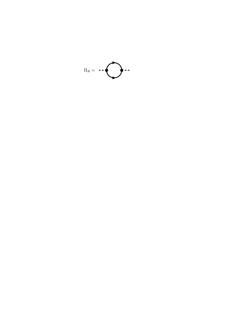
Figure 1: The Feynman diagrams for the Higgs polarization function $\Pi_{H}$.

Evaluating the one-loop quark-quark bubble $\Pi_{H}(k)$ shown in Fig. 1, we obtain that

$$\Pi_{H}(k)=\frac{2\bar{\mu}^{2}}{\pi}I(k|\delta\mu)+\frac{\bar{\mu}^{2}}{2\pi\Delta^{2}}k^{2}J(k|\delta\mu),$$ (53)

where the functions $I(k|\delta\mu)$ and $J(k|\delta\mu)$ are given by

$$I(k|\delta\mu)=\Delta^{2}T\sum_{n}\frac{1}{\sqrt{(\omega_{n}+i\delta\mu)^{2}+\Delta^{2}}}\int_{-1}^{1}dx\frac{1}{(\omega_{n}+i\delta\mu)^{2}+\Delta^{2}+\frac{1}{4}k^{2}x^{2}},$$ (54)

$$J(k|\delta\mu)=\Delta^{2}T\sum_{n}\frac{1}{\sqrt{(\omega_{n}+i\delta\mu)^{2}+\Delta^{2}}}\int_{-1}^{1}dx\frac{x^{2}}{(\omega_{n}+i\delta\mu)^{2}+\Delta^{2}+\frac{1}{4}k^{2}x^{2}}.$$ (55)

with ${\rm Re}\sqrt{(\omega_{n}+i\delta\mu)^{2}+\Delta^{2}}>0$. Here, the summation over $n$ is the frequency summation at finite temperature field theory, with $\omega_{n}=(2n+1)\pi T$. At T=0, both functions can be simplified as shown in the appendices A and B. Their power series expansion yield

$$\Pi_{H}(k)=A_{H}+B_{H}k^{2}$$ (56)

with

$$A_{H}=\left(\frac{\partial^{2}\Omega_{M}}{\partial\Delta^{2}}\right)_{\delta\mu}=\frac{4\bar{\mu}^{2}}{\pi^{2}}\Big{(}1-\frac{\delta\mu}{\sqrt{(\delta\mu)^{2}-\Delta^{2}}}\Big{)},$$ (57)

$$B_{H}=\frac{2\bar{\mu}^{2}}{9\pi^{2}\Delta^{2}}\Big{[}1-\frac{(\delta\mu)^{3}}{((\delta\mu)^{2}-\Delta^{2})^{\frac{3}{2}}}\Big{]}.$$ (58)

It follows from Eqs. (57) and (58) that the Higgs field becomes unstable in the gapless phase when $\delta\mu>\Delta$, $A_{H}$ in the gapless phase is shown in Fig. 3 by the red dash-dotted line. The Higgs instability was also considered in Ref. Kei-Kenji , where it was called as ”amplitude instability”. It has to be pointed out that we got different expressions for the coefficients of the gradient term. For $k>>\Delta$, we have

$$\Pi_{H}(k)\simeq\frac{\bar{\mu}^{2}}{2\pi^{2}}\Big{(}2\ln\frac{k}{\Delta}-2-\ln\frac{\delta\mu-\sqrt{\delta\mu^{2}-\Delta^{2}}}{\delta\mu+\sqrt{\delta\mu^{2}-\Delta^{2}}}\Big{)}.$$ (59)

Therefore the Higgs instability disappears for sufficiently large momentum. The form factor $\Pi_{H}(k)$ for arbitrary momentum is plotted using red dashed line in Fig. 4 for a typical value of the mismatch parameter $\Delta/\delta\mu=1/2$. We notice that the Higgs instability becomes stronger for nonzero momentum.

Near the transition temperature, $\Delta<<T$, we may drop $\Delta$’s inside the square roots and in the denominators on RHS of Eqs. (54) and (55). The Higgs self-energy function (53) goes to the expression derived from the Ginzburg-Landau theory Type-trans . The Ginzburg-Landau free energy for g2SC can be easily obtained from that of an electronic superconductor by replacing the Fermi momentum $k_{F}$ with $\bar{\mu}$, the Fermi velocity with one and multiplying the whole expression by four (four pairing configurations per momentum for g2SC versus one for the electronic SC).

We would like to make two remarks before concluding this section: 1) The combination of $\vec{A}-\frac{1}{g}\vec{\nabla}\varphi$ of Eq. (47) is by no means generic for a nonrelativistic system. The general expression of $\Omega_{NG}$ beyond the long wavelength limit takes the form

$$\Omega_{NG}=\frac{1}{2}\int\frac{d^{3}\vec{k}}{(2\pi)^{3}}\sum_{a=1}^{8}\left[\Pi_{a}^{\perp}(k){\vec{\bf A}}_{\perp}^{a*}(\vec{k})\cdot{\vec{\bf A}}_{\perp}^{a}(\vec{k})+\Pi_{a}^{||}(k)({\vec{\bf A}}_{||}^{a*}+\frac{i}{g}\vec{k}\varphi^{a*}(\vec{k}))\cdot({\vec{\bf A}}_{||}^{a}(\vec{k})-\frac{i}{g}\vec{k}\varphi^{a}(\vec{k}))+higher\,orders\,\right].$$ (60)

in momentum representation, where $\vec{A}_{||}$($\vec{A}_{\perp}$) is parallel(perpendicular) to $\vec{k}$. Except that $\Pi_{a}^{\perp}(0)=\Pi_{a}^{||}(0)$, they may be quite different for $\vec{k}\neq 0$, so are the instability domains with respect to $k$. 2) At $T=0$, the dependence of the thermodynamic function on the diquark field is highly nonlinear and the gradient term is not Ginzburg-Landua like, i.e., $\vec{\nabla}\Delta^{\rho*}\cdot\vec{\nabla}\Delta^{\rho}$. There are no simple relations between the coefficient $B_{H}$ and the Meissner mass squares. This may explain the difference between our $B_{H}$ and that of Kei-Kenji .

IV A General View of the Higgs Instability

In this section, we shall provide a general view of the Higgs instability in relation to the Sarma instability as well as the Coulomb energy in relation to the charge neutrality constraint. Consider a system described by the Hamiltonian ${\cal H}$ with a spontaneous symmetry breaking. The thermodynamic potential is given by

$$\Omega=-T\ln{\rm Tr}\exp\left(-\frac{{\cal H}-\sum_{j=1}^{m}\mu_{j}Q_{j}}{T}\right)$$ (61)

where $Q$’s are $m$ conserved charges with $\mu$’s the corresponding chemical potentials. The trace extends to a subset of the Hilbert space specified by $n$ order parameters $\Delta_{a}$ with $a=1,...,n$, which are invariant under the symmetry group of ${\cal H}$ and are homogeneous. In the mean field approach, one approximates ${\cal H}$ with ${\cal H}_{\rm MF}$ that depends on the order parameters explicitly and leaves the trace unrestricted. In the superfluid of imbalanced atoms or in g2SC, we have $m=2$ and $n=1$. $Q_{1}$ and $Q_{2}$ stand for the number of atoms of each species in the former or the electric charge and the 8th color charge in the latter. $\Delta_{1}$ corresponds to the magnitude of the gap parameter in both cases. In particular, $\Delta_{1}\equiv\Delta$ of the last two sections. For gCFL, $m=n=3$ with $Q_{1}$, $Q_{2}$ and $Q_{3}$ the electric, 3rd color and 8th color charges while $\Delta_{1}$, $\Delta_{2}$ and $\Delta_{3}$ correspond to the magnitude of the eigenvalues of the $3\times 3$ diquark condensate matrix $\Phi_{f}^{c}\equiv\epsilon^{cc_{1}c_{2}}\epsilon_{ff_{1}f_{2}}<q_{f_{1}}^{c_{1}}q_{f_{2}}^{c_{2}}>$. The equilibrium conditions read

$$\Big{(}\frac{\partial\Omega}{\partial\Delta_{a}}\Big{)}_{\nu_{1},...,\nu_{m}}=0.$$ (62)

and the expectation value of the $Q$-quanta density reads

$$n_{j}=\frac{1}{V}<Q_{j}>=-\Big{(}\frac{\partial\Omega}{\partial\mu_{j}}\Big{)}_{\Delta_{1},...,\Delta_{n}}$$ (63)

where $V$ is the volume of the system and the thermal average $<Q_{j}>$ is defined as

$$<Q_{j}>=\frac{{\rm Tr}Q_{j}\exp\left(-\frac{{\cal H}-\sum_{j=1}^{m}\mu_{j}Q_{j}}{T}\right)}{{\rm Tr}\exp\left(-\frac{{\cal H}+\sum_{j=1}^{m}\mu_{j}Q_{j}}{T}\right)}.$$ (64)

The Sarma instability corresponds to the negative eigenvalues of the $n\times n$ stability matrix

$$\Big{(}\frac{\partial^{2}\Omega}{\partial\Delta_{a}\partial\Delta_{b}}\Big{)}_{\mu_{1},...,\mu_{n}}.$$ (65)

Under the constraints of fixed densities $n_{j}$’s, the relevent thermodynamic quantity to be minimized is the Helmholtz free energy which is obtained by a Legendre transformation,

$${\cal F}=\Omega+\sum_{j}\mu_{j}n_{j}.$$ (66)

While the equilibrium conditions

$$\Big{(}\frac{\partial{\cal F}}{\partial\Delta_{a}}\Big{)}_{n_{1},...,n_{m}}=0.$$ (67)

are equivalent to Eq. (62), the stability matrix becomes

$$\Big{(}\frac{\partial^{2}{\cal F}}{\partial\Delta_{a}\partial\Delta_{b}}\Big{)}_{n_{1},...,n_{m}}=\Big{(}\frac{\partial^{2}\Omega}{\partial\Delta_{a}\partial\Delta_{b}}\Big{)}_{\mu_{1},...,\mu_{m}}+\sum_{ij}(M^{-1})_{ij}\Big{(}\frac{\partial Q_{i}}{\partial\Delta_{a}}\Big{)}_{\mu_{1},...,\mu_{m}}\Big{(}\frac{\partial Q_{j}}{\partial\Delta_{b}}\Big{)}_{\mu_{1},...,\mu_{m}}.$$ (68)

where the $m\times m$ matrix

$$M_{ij}=-\Big{(}\frac{\partial^{2}\Omega}{\partial\mu_{i}\partial\mu_{j}}\Big{)}_{\Delta_{1},...,\Delta_{n}}$$ (69)

is positive. To see this point, we carry out the second order derivative and obtain that

$$M_{ij}=<Q_{i}Q_{j}>-<Q_{i}><Q_{j}>=<(Q_{i}-<Q_{i}>)(Q_{j}-<Q_{j}>)>.$$ (70)

The positivity follows from the observation that $z^{\dagger}Mz>0$ for an arbirary $m\times 1$ complex column matrix $z$. Therefore, the stability matrix (68) could be positive even Eq. (65) is not so. This is precisely what the constraint of fixed particle numbers in case of BP or the constraint of the charge neutrality accomplished. Because of the relations (63) and

$$\mu_{j}=\left(\frac{\partial{\cal F}}{\partial n_{j}}\right)_{\Delta_{1},...,\Delta_{n}},$$ (71)

we have

$$M_{ij}=\left(\frac{\partial n_{i}}{\partial\mu_{j}}\right)_{\Delta_{1},...,\Delta_{n}}$$ (72)

and

$$(M^{-1})_{ij}=\left(\frac{\partial\mu_{i}}{\partial n_{j}}\right)_{\Delta_{1},...,\Delta_{n}}=\left(\frac{\partial^{2}{\cal F}}{\partial n_{i}\partial n_{j}}\right)_{\Delta_{1},...,\Delta_{n}}.$$ (73)

Therefore the positivity of $M_{ij}$ also implies that of the matrix

$$\left(\frac{\partial^{2}{\cal F}}{\partial n_{i}\partial n_{j}}\right)_{\Delta_{1},...,\Delta_{n}}.$$ (74)

The inclusion of inhomogeneous variations renders the stability matrix infinitely dimensional with additional matrix elements

$$\Big{(}\frac{\partial^{2}{\cal F}}{\partial\phi_{a}^{*}(\vec{k})\partial\phi_{b}(\vec{k})}\Big{)}_{n_{1},...,n_{m}}=\Big{(}\frac{\partial^{2}\Omega}{\partial\phi_{a}^{*}(\vec{k})\partial\phi_{b}(\vec{k})}\Big{)}_{\mu_{1},...,\mu_{m}}$$ (75)

at $\vec{k}\neq 0$, without the second term of Eq. (68), where we have parametrized a general variation of the order parameters according to

$$\delta\Delta_{a}+\frac{1}{V}\sum_{\vec{k}\neq 0}\delta\phi_{a}(\vec{k})e^{i\vec{k}\cdot\vec{r}}$$ (76)

with $V$ the volume of the system. If the matrix elements Eq. (75) are not singular at $\vec{k}=0$ in the thermodynamic limit, $V\to\infty$,

$$\lim_{\vec{k}\to 0}\lim_{V\to\infty}\Big{(}\frac{\partial^{2}\Omega}{\partial\phi_{a}^{*}(\vec{k})\partial\phi_{b}(\vec{k})}\Big{)}_{\mu_{1},...,\mu_{m}}=\Big{(}\frac{\partial^{2}\Omega}{\partial\Delta_{a}\partial\Delta_{b}}\Big{)}_{\mu_{1},...,\mu_{m}}$$ (77)

The Sarma instability will show up with respect to the variations of a sufficiently low but nonzero momentumn.

The Higgs instability can also be understood intuitively. Let us devide the whole system being considered into ${\cal N}$ subsystems of equal volumes and equal chemical potentials. We label them by the integer $p$. As long as the size of each subsystem is much larger than all microscopic length scales, the energy of the interfaces can be ignored. At equilibrium, the thermodynamic potential density of the master system is

$$\Omega^{\rm tot.}=\frac{1}{{\cal N}}\sum_{p}\Omega^{(p)}=\Omega_{M}$$ (78)

where $\Omega_{M}$ is given by (44) with $\Delta$ by (45). Now we consider an inhomogeneous variation of the gap parameters, $\delta\Delta_{1}^{(p)},...,\delta\Delta_{n}^{(p)}$, such that 1) each of the $n$-component vector, $(\Delta_{1}^{(p)},...,\Delta_{n}^{(p)})$ proportional to the same eigenvector of the matrix

$$\left(\frac{\partial^{2}\Omega}{\partial\Delta_{a}\partial\Delta_{b}}\right)_{\mu_{1},...,\mu_{m}}$$ (79)

with the negative eigenvalue $\lambda<0$, 2) $\sum_{p}\delta\Delta_{a}^{(p)}=0$. Then

$$\delta n_{j}=\frac{1}{{\cal N}}\sum_{a,p}\frac{\partial n_{j}}{\partial\Delta_{a}}\delta\Delta_{a}^{(p)}=\frac{1}{{\cal N}}\sum_{a}\frac{\partial n_{j}}{\partial\Delta_{a}}\sum_{p}\delta\Delta_{a}^{(p)}=0$$ (80)

but

$$\delta\Omega^{\rm tot.}\simeq\frac{1}{{\cal N}}\sum_{a,b}\frac{\partial^{2}\Omega}{\partial\Delta_{a}\partial\Delta_{b}}\sum_{p}\delta\Delta_{a}^{(p)}\delta\Delta_{b}^{(p)}=\frac{1}{{\cal N}}\lambda\sum_{a,p}\delta\Delta_{a}^{(p)}\delta\Delta_{a}^{(p)}<0.$$ (81)

Therefore the Sarma instability develops through different variations of the order parameters of each susystem while maintaining the constraint conditions of the master system.

V Coulomb Energy

Unless a competing mechanism that results in a positive contribution to the inhomogeneous blocks of the stability matrix. The Higgs instability will prevent gapless superfluidity/ superconductivity from being implemented in nature. In the system of imbalanced neutral atoms, such a mechanism is not likely to exist and this contributes to the reason why the BP state has never been observed there. For the quark matter being considered, however, the positive Coulomb energy induced by the Higgs field of electrically charged diquark pairs has to be examined.

The second order derivative of the Hemlholtz free energy, Eq. (68) for g2SC reads:

$$\Big{(}\frac{\partial^{2}{\cal F}}{\partial\Delta^{2}}\Big{)}_{n_{e}}=\Big{(}\frac{\partial^{2}\Omega}{\partial\Delta^{2}}\Big{)}_{\mu_{e}}+\frac{\Big{(}\frac{\partial n_{e}}{\partial\Delta}\Big{)}_{\mu_{e}}^{2}}{\Big{(}\frac{\partial n_{e}}{\partial\mu_{e}}\Big{)}_{\Delta}}$$ (82)

and the stability implemented by the charge neutrality implies that

$$\Big{(}\frac{\partial^{2}{\cal F}}{\partial\Delta^{2}}\Big{)}_{n_{e}}>0.$$ (83)

While the global charge neutrality is maintained, an inhomogeneous $\phi$ will induce local charge distribution. The corresponding Coulomb energy

$$E_{\rm coul.}=\frac{1}{2}\sum_{\vec{k}\neq 0}\frac{\delta\rho(\vec{k})^{*}\delta\rho(\vec{k})}{k^{2}+m_{D}^{2}(k)},$$ (84)

should be added to the RHS of the stability matrix element (75) where $\delta\rho(\vec{k})$ is the Fourier component of the $\phi$-induced charge density and $m_{D}$ is the Coulomb polarization function ( Debye mass at $\vec{k}=0$ ). We have

$$m_{D}^{2}(k)=-\frac{e^{2}T}{2}\sum_{P}{\rm tr}\gamma_{0}Q{\cal S}(P+K)\gamma_{0}Q{\cal S}(P)$$ (85)

and

$$\delta\rho(\vec{k})=\kappa(k)H(\vec{k}),$$ (86)

where

$$\kappa(k)=\frac{ieT}{2}\sum_{P}{\rm tr}\gamma_{0}Q{\cal S}(P+K)\gamma_{5}\epsilon^{3}\rho_{2}{\cal S}(K)$$ (87)

with $K=(0,\vec{k})$ and $Q$ the electric charge operator. We have

$$Q=\rho_{3}(a+b\tau_{3})$$ (88)

with $a=1/6$ and $b=1/2$ for the quark matter consisting of $u$ and $d$ flavors. The Eq. (84) corresponds to the diagram $a$ of Fig. 2. The diagram $b$ in Fig. 2 represents the exchange Coulomb energy and is ignored since the typical momentum running through the Coulomb line of the order $\bar{\mu}$ compared that in the first diagram, $m_{D}\sim\alpha_{e}\bar{\mu}$. It is shown in appendix C that the Goldstone fields do not generate electric charge distributions.

Figure 2: $a$ is the Coulomb Energy in Eq. (84), and $b$ is the ignored exchange Coulomb energy.

The inhomogeneous block of the stability matrix element, (75), becomes now

$$\tilde{\Pi}_{H}(k) \equiv \Big{(}\frac{\partial^{2}{\cal F}}{\partial H^{*}(\vec{k})\partial H(\vec{k})}\Big{)}_{n_{e}}=\Big{(}\frac{\partial^{2}\Omega}{\partial H^{*}(\vec{k})\partial H(\vec{k})}\Big{)}_{\mu_{e}}+\frac{\kappa^{*}(k)\kappa(k)}{k^{2}+m_{D}^{2}(k)}$$

$$= \Pi_{H}(k)+\frac{\kappa^{*}(k)\kappa(k)}{k^{2}+m_{D}^{2}(k)}.$$

The stability of the system with respect to the Higgs field requires that $\tilde{\Pi}_{H}(k)>0$ for all $k$.

The form factor $\kappa(q)$ and the momentum dependent Debye mass square can be calculated explicitly at weak coupling, i.e. $\delta\mu<<\bar{\mu}$ and $k<<\bar{\mu}$. We find that

$$\kappa(k)=\frac{2e^{2}\bar{\mu}^{2}b}{\pi}K(k|\delta\mu)$$ (90)

with

$$K(k|\delta\mu)=i\Delta T\sum_{n}\frac{\omega_{n}+i\delta\mu}{\sqrt{(\omega_{n}+i\delta\mu)^{2}+\Delta^{2}}}\int_{-1}^{1}dx\frac{1}{(\omega_{n}+i\delta\mu)^{2}+\Delta^{2}+\frac{1}{4}k^{2}x^{2}}$$ (91)

and

$$m_{D}^{2}(k)=\frac{6(a^{2}+b^{2})e^{2}\bar{\mu}^{2}}{\pi^{2}}-\frac{2b^{2}e^{2}\bar{\mu}^{2}}{\pi}I(k|\delta\mu)$$ (92)

with the first term the Debye mass of the normal phase and $I(q|\delta\mu)$ the function defined in the section III.

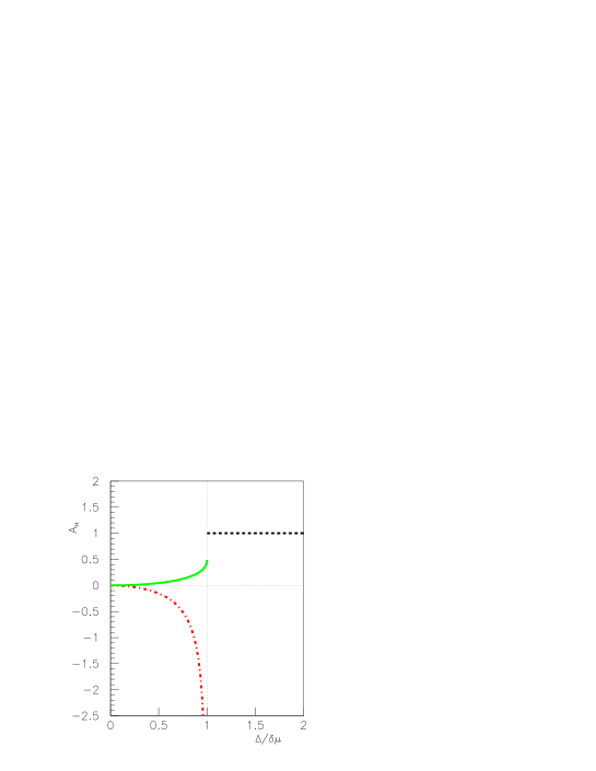
Figure 3: $A_{H}$(red dashed-dotted line) and $\tilde{A}_{H}$ (green solid line) are plotted as functions of $\Delta/\delta\mu$ in the g2SC phase, and the black dashed line shows the corresponding quantity in the 2SC phase.

Zero momentum limit:

Notice that

$$\lim_{k\to 0}\lim_{V\to\infty}\Big{(}\frac{\partial^{2}\Omega}{\partial H^{*}(\vec{k})\partial H(\vec{k})}\Big{)}_{\mu_{Q}}=\Big{(}\frac{\partial^{2}\Omega}{\partial\Delta^{2}}\Big{)}_{\mu_{Q}},$$ (93)

$$m_{D}^{2}(0)=e^{2}\Big{(}\frac{\partial n_{e}}{\partial\mu_{e}}\Big{)}_{\Delta,\mu_{B}}$$ (94)

and

$$\kappa(0)=e\Big{(}\frac{\partial n_{e}}{\partial\Delta}\Big{)}_{\mu_{e},\mu_{B}}.$$ (95)

We have

$$\lim_{\vec{k}\to 0}\Big{(}\frac{\partial^{2}{\cal F}}{\partial H^{*}(\vec{k})\partial H(\vec{k})}\Big{)}_{\mu_{e}}=\Big{(}\frac{\partial^{2}{\cal F}}{\partial\Delta^{2}}\Big{)}_{\mu_{e}},$$ (96)

and the charge neutrality stabilize also the inhomogeneous Higgs field with the momentum much smaller than the inverse coherence length and the inverse Debye length.

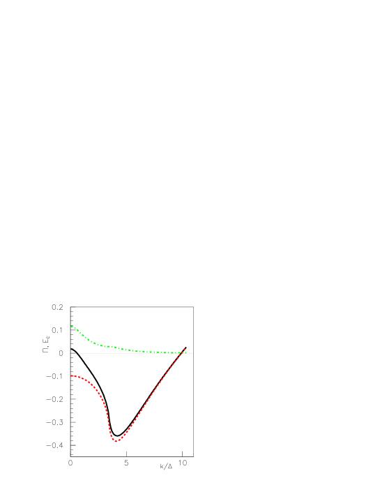
Figure 4: The function $\Pi_{H}(k)$ (red dashed line), $\tilde{\Pi}_{H}(k)$ (black solid line) and the Coulomb energy (green dash-dotted line) as functions of scaled-momentum $k/\Delta$, in the case of $\delta\mu=2\Delta$ and $(e^{2}\bar{\mu}^{2})/(4\pi\Delta^{2})=1$.

In the static long-wave length limit, we have

$$m_{D}^{2}(0)=\frac{2e^{2}b^{2}\bar{\mu}^{2}}{\pi^{2}}\Big{(}1+\frac{2\delta\mu}{\sqrt{\delta\mu^{2}-\Delta^{2}}}\Big{)}$$ (97)

and

$$\kappa(0)=\frac{4eb\bar{\mu}^{2}}{\pi^{2}}\frac{\Delta}{\sqrt{\delta\mu^{2}-\Delta^{2}}}.$$ (98)

The positivity of the Debye mass square is ensured by the positivity of the $M$- matrix defined in (69). It follows from Eqs. (46), (V), (97) and (98) that the Higgs self-energy including Coulomb energy correction

$${\tilde{A}}_{H}\equiv\tilde{\Pi}_{H}(0)=\Big{(}\frac{\partial^{2}{\cal F}}{\partial\Delta^{2}}\Big{)}_{\mu,n_{Q}}=\frac{4(b^{2}-3a^{2})\bar{\mu}^{2}(\delta\mu-\sqrt{\delta\mu^{2}-\Delta^{2}})}{\pi^{2}[3a^{2}\sqrt{\delta\mu^{2}-\Delta^{2}}+b^{2}(2\delta\mu+\sqrt{\delta\mu^{2}-\Delta^{2}})]}$$ (99)

is always positive for the whole range of g2SC state. It means that the Sarma instability in the gapless phase can be cured by Coulomb energy. This is shown in Fig. 3, where the red dash-dotted line indicates the $A_{H}$ and the green solid line indicates ${\tilde{A}}_{H}$.

Nonzero momentum case:

While the Sarma instability in g2SC phase can be cured by Coulomb energy under the constraint of charge neutrality condition, it is not sufficient for the system to be stable, even if the chromomagnetic instabilities are removed, say by gluon condensation. One has to explore the Higgs instability by calculating the self-energy function $\tilde{\Pi}(k)$ in the whole momentum space, which amounts to value the three basic functions $I(k|\delta\mu)$, $J(k|\delta\mu)$ and $K(k|\delta\mu)$ defined in (54), (55) and (91). At $T=0$, the summation over Matsubara frequencies becomes an integral and we have

$$I(k|\delta\mu)=\frac{\Delta^{2}}{2\pi}\int_{-1}^{1}dx\Big{(}\int_{-\infty+i\delta\mu}^{i\delta\mu-0^{+}}+\int_{i\delta\mu+0^{+}}^{\infty+i\delta\mu}\Big{)}dz\frac{1}{\sqrt{z^{2}+\Delta^{2}}\Big{(}z^{2}+\Delta^{2}+\frac{1}{4}k^{2}x^{2}\Big{)}}$$ (100)

$$J(k|\delta\mu)=\frac{\Delta^{2}}{2\pi}\int_{-1}^{1}dxx^{2}\Big{(}\int_{-\infty+i\delta\mu}^{i\delta\mu-0^{+}}+\int_{i\delta\mu+0^{+}}^{\infty+i\delta\mu}\Big{)}dz\frac{1}{\sqrt{z^{2}+\Delta^{2}}\Big{(}z^{2}+\Delta^{2}+\frac{1}{4}k^{2}x^{2}\Big{)}}$$ (101)

and

$$K(k|\delta\mu)=\frac{i\Delta}{2\pi}\int_{-1}^{1}dx\Big{(}\int_{-\infty+i\delta\mu}^{i\delta\mu-0^{+}}+\int_{i\delta\mu+0^{+}}^{\infty+i\delta\mu}\Big{)}dz\frac{z}{\sqrt{z^{2}+\Delta^{2}}\Big{(}z^{2}+\Delta^{2}+\frac{1}{4}k^{2}x^{2}\Big{)}}.$$ (102)

Further reductions of these integrals are straightforward but rather technical. The details are deferred to Appendix B. Here we present only the numerical results in Fig. 4 and Table I.

Fig. 4 shows the Higgs self-energy $\Pi_{H}(k)$ (the red dashed line) the Coulomb corrected Higgs self-energy ${\tilde{\Pi}}_{H}(k)$ (the black solid line) and the Coulomb energy $E_{coul}$ (the green dash-dotted line) as functions of scaled-momentum $k/\Delta$, in the case of $\delta\mu=2\Delta$ and $(e^{2}\bar{\mu}^{2})/(4\pi\Delta^{2})=1$.

Eventhough the Higgs instability can be removed by the Coulomb energy for small momenta, it returns for intermediate momenta. This phenomenon persists for a wide range of gap magnitude, $0<\Delta<0.866\delta\mu$ and for all strength of the Coulomb interaction, measured by the dimensionless ration $\eta\equiv\frac{\alpha_{e}\bar{\mu}^{2}}{\Delta^{2}}$. Within the narrow range $0.866\delta\mu<\Delta<\delta\mu$, the Higgs instability could be removed if the Coulomb interaction were sufficiently strong. For $\eta=1$, We found that $\tilde{\Pi}_{H}(k)>0$ for all $k$ if $0.998\delta\mu<\Delta<\delta\mu$. In terms of the values of the parameters of NJL model, we have $\alpha_{e}\bar{\mu}^{2}<\delta\mu$. Therefore the electric Coulomb energy cannot cure the Higgs instability for a realistic two flavor quark matter.

Negative $\Pi_{H}(k)$ indicates the Higgs mode is unstable and will decay Coleman-Weinberg . It is noticed that $\Pi_{H}(k)$ reaches its minimum at a momentum, i.e., $k\simeq 4\Delta$, which indicates that a stable state may develop around this minimum, we characterize this momentum as $k_{min}$. The inverse $k_{min}^{-1}$ is the typical wavelength for the unstable mode Weinberg-Wu . If mixed phase can be formed, the typical size $l$ of the 2SC bubbles should be as great as $k_{min}^{-1}$, i.e., $l\simeq k_{min}^{-1}$ Weinberg-Wu , which turns out to becomparable to the coherence length of 2SC in accordance with Eq. (45). (In the case of homogeneous superconducting phase, $k_{min}=0$, and $l\rightarrow\infty$.) Considering that the coherence length $\xi$ of a superconductor is proportianl to the inverse of the gap magnitude, i.e., $\xi\simeq\Delta^{-1}$ Type-trans , therefore, a rather large ratio of $k_{min}/\Delta$ means a rather small ratio of $l/\xi$. When $l/\xi<1$, a phase separation state is more favorable Igor .

$\delta\mu/\Delta$	$\alpha_{e}\Delta^{2}/\bar{\mu}^{2}$	$\tilde{\Pi}(0)$	$\tilde{\Pi}_{\rm min}(k)$	$k_{\rm min}/\Delta$	$k_{\rm min}/\Delta_{0}$
5	0.25	0.0026	-0.2778	11.72	1.18
5	1	0.0026	-0.2774	11.71	1.18
5	4	0.0026	-0.2763	11.71	1.18
2	0.25	0.0180	-0.3760	4.12	1.10
2	1	0.0180	-0.3592	4.12	1.10
2	4	0.0180	-0.3148	4.12	1.10
1.25	0.25	0.0606	-0.6377	1.78	0.89
1.25	1	0.0606	-0.4185	1.78	0.89
1.25	4	0.0606	-0.2045	1.78	0.89

Table 1: The minimum of the self-energy of Higgs field for various mismatch parameters and strengths of Coulomb interaction.

In Table 1, we show the Coulomb corrected Higgs self-energy at zero momentum $\tilde{\Pi}_{H}(0)$, its minimum, the corresponding $k_{min}/\Delta$ and $k_{\rm min}/\Delta_{0}$ ( with $\Delta$ and $\Delta_{0}$ related by eq. (45) for different parameters of $\Delta/\delta\mu$ and $\alpha_{e}\Delta^{2}/\bar{\mu}^{2}$. It is found that the momentum for the Higgs self-energy to reach minimun is not sensitive to the electromagnetic coupling strength, rather very sensitive to the ratio of $\delta\mu/\Delta$. Larger $\delta\mu/\Delta$ is, larger $k_{min}/\Delta$ will be. But the ratio of this momentum to the gap of 2SC under the same pairing strength is close to one for all cases being examined.

The reader has to keep in mind that our result of the Higgs instability only indicates some kind of inhomogeneous states whose typical length scale is comparable to the coherence length of 2SC. Further insight on the structure of the inhomogeneity cannot be gained without exploring the higher order terms of the nonlinear realization (25). A more direct approach to obtain the favorite structure of the ground state is to compare the free energy of various candidate states, which include the mixed phase, the single-plane wave FF state, striped LO state and multi-plane wave states. The Coulomb energy and the gradient energy have to be estimated reliably. We leave this analysis as a future project.

VI Summary and overlook

To understand the pair-breaking superfluidity or superconductivity induced by mismatched Fermi momenta, one has to go beyond the standard framework of BCS theory. In this paper, we offered a nonlinear realization framework of the gauged Nambu–Jona-Lasinio model, where the fluctuations of the Higgs and pseudo Nambu-Goldstone fields can be investigated simutaneously.

It is found that, with the increase of mismatch between the Fermi surfaces of the pairing quarks, not only Nambu-Goldstone currents can be spontaneously generated, but the Higgs filed becomes unstable in the gapless phase. As we already knew, the instability of the Nambu-Goldstone currents naturally induce the formation of the single-plane wave FF state. In this paper, we focused on the Higgs instability which has not drawn much attention yet.

The Higgs instability is the origin of spatial inhomogeneity, and is not prohibited by global constraints. In the case of the imbalanced neutral atom systems, the instability extends from arbitrarily low momenta-albeit not zero-to momenta much higher than the inverse coherence length. Without a long range force a macroscopic phase separation is likely to be the structure of the ground state since it minimizes the gradient energy of the inhomogeneity without additional costs. The thermodynamics of the phase separation can be obtained following the Gibbs construction of gibbs .

For the case of two flavor quark matter that is globally neutral, the instability is absent for high momenta and can be removed by the electric Coulomb energy for low momenta. But it remains in a window of intermediate momenta. In the regime where $\delta\mu>>\Delta$, the wavelength for the unstable Higgs mode is alway comparable with the gap magnitude of 2SC phase, which indicates the tendency to form 2SC bubbles. Because of the Long range Coulomb force, a macroscopic phase separation is prohibited while a crystalline structure is more favorable. Possible candidates include the heterotic mixture of normal and superconducting phases and the multi-plane-wave LOFF state.

Although our calculations are limited to the case of g2SC, the existence of the Higgs instability in the absence of long range interactions is generic for all gapless superfluidity/superconductivity that are subject to the Sarma instability. Our general formulation can be readily applied to the system with several invariant order parameters and constraints. It would be interesting to examine whether the electric and color Coulomb energies are capable of eliminating the Higgs instability completely in the gCFL phase.

It is quite surprising that the Higgs instability shows up at some finite momentum, though it is removed by the constraint of the charge neutrality. Following the discovery of the chromomagnetic instability of g2SC at $T=0$, the authors of wangqh examined the Meissner mass square at $T\neq 0$ and found that the instability goes away for $T$ sufficiently close to $T_{c}$. In the light of our result of the Higgs instability, this criterion is not sufficient for the stability. One has to extend the analysis of wangqh to all momenta of the chromomagnetic polarization function as well as that of the Higgs self-energy function at $T\neq 0$ in order to map out the stability domain of g2SC in the phase diagram of the two flavor quark matter. This amounts to value the functions $I(k|\delta\mu)$, $J(k|\delta\mu)$ and $K(k|\delta\mu)$ at nonzero $T$, which is straightforward. We hope to report our progress in this direction in near future.

Appendix A Calculation of $\Pi_{H}(k)$ and $\tilde{\Pi}_{H}(k)$

The calculation of the one-loop self energies of the inhomogeneously fluctuating fileds introduced in Section III and V will be illurstrated in this appendix with that of the Higgs field, given by

$$\Pi_{H}(k)=\frac{1}{2G_{D}}-\frac{1}{2}T\sum_{n}\int\frac{d^{3}\vec{p}}{(2\pi)^{3}}{\rm Tr}\epsilon^{3}\rho_{2}\tau_{2}{\cal S}_{M}(\omega_{n},\vec{p}+\vec{k})\epsilon^{3}\rho_{2}\tau_{2}{\cal S}_{M}(\omega_{n},\vec{p}),$$ (103)

where we exihibite the dependence of the propagator on momentum and Matsubara energy separately. It is convenient to tranform the propagator into the representation of Ref. FF-Ren via

$${\cal S}_{M}(\omega,\vec{p})\equiv U{\cal S}(\omega,\vec{p})U^{\dagger}$$ (104)

where $U=\rho_{+}+\rho_{-}\tau_{2}$ with $\rho_{\pm}=\frac{1}{2}(1\pm\rho_{3})$. It follows that

$${\cal S}(\omega,\vec{p})^{-1}=i\omega\gamma_{0}-\vec{\gamma}\cdot\vec{p}+\bar{\mu}\gamma_{0}\rho_{3}-\delta\mu\gamma_{0}\tau_{3}+\Delta\gamma_{5}\epsilon^{3}\rho_{2},$$ (105)

where we have suppressed the chemical potential associated to the 8th color. Correspondingly,

$$\Pi_{H}(k)=\frac{1}{2G_{D}}-\frac{1}{2}T\sum_{n}\int\frac{d^{3}\vec{p}}{(2\pi)^{3}}{\rm Tr}\epsilon^{3}\rho_{2}{\cal S}(\omega_{n},\vec{p}+\vec{k})\epsilon^{3}\rho_{2}{\cal S}(\omega_{n},\vec{p}),$$ (106)

where the matrix under the trace is diagonal in isospin space and the trace with respect to iospins becomes the sum over the eigenvalue of $\tau_{3}$.

With respect to the color indexes r, g and b,

$$\epsilon^{3}=\left(\begin{array}[]{cc}i\sigma_{2}&0\\ 0&0\end{array}\right)$$ (107)

with $\sigma_{2}$ the second Pauli matrix in the color SU(2) subspace. Accordingly,

$$\Pi_{H}(k)=\frac{1}{2G_{D}}-\frac{1}{2}T\sum_{n}\int\frac{d^{3}\vec{p}}{(2\pi)^{3}}{\rm Tr}\epsilon^{3}\rho_{2}{\cal S}^{SU(2)}(\omega_{n},\vec{p}+\vec{k})\epsilon^{3}\rho_{2}{\cal S}^{SU(2)}(\omega_{n},\vec{p}),$$ (108)

with ${\cal S}^{SU(2)}$ the color SU(2) block of the propagator. The expression of ${\cal S}^{SU(2)}$ can be obtained from (105) with the replacement of $\epsilon^{3}$ by $i\sigma_{2}$. The trace in color space extends only to r and g indexes now.

On writing

$$[{\cal S}^{SU(2)}(\omega,\vec{p})]^{-1}=\gamma_{0}\rho_{3}[\rho_{3}(i\omega-\vec{\alpha}\cdot\vec{p})+\bar{\mu}-\delta\mu\rho_{3}\tau_{3}+i\Delta\gamma_{0}\gamma_{5}\sigma_{2}\rho_{1}],$$ (109)

we notice that the matrix (…) can be projected into two orthogonal subspace via

$$\Lambda_{\pm}=\frac{1}{2}(1\pm\rho_{3}\vec{\alpha}\cdot\hat{p})$$ (110)

with $\vec{\alpha}=\gamma_{0}\vec{\gamma}$. We find that

$$(i\omega-\vec{\alpha}\cdot\vec{p})\rho_{3}+\bar{\mu}-\delta\mu\rho_{3}\tau_{3}+i\Delta\gamma_{0}\gamma_{5}\sigma_{2}\rho_{1}$$ (111)

$$= \Lambda_{+}(i\omega\rho_{3}-p+\bar{\mu}-\delta\mu\rho_{3}\tau_{3}+i\Delta\gamma_{0}\gamma_{5}\sigma_{2}\rho_{1})+\Lambda_{-}(i\omega\rho_{3}+p+\bar{\mu}-\delta\mu\rho_{3}\tau_{3}+i\Delta\gamma_{0}\gamma_{5}\sigma_{2}\rho_{1}).$$

Under the weak coupling approximation, $\omega<<\bar{\mu}$, $|p-\bar{\mu}|<<\bar{\mu}$, $\Delta<<\bar{\mu}$ and $\delta\mu<<\bar{\mu}$, The contribution of the second term to the inverse can be ignored. We obtains that

$${\cal S}_{M}^{SU(2)}(\omega,\vec{p})\simeq\Lambda_{+}(i\omega\rho_{3}-p+\bar{\mu}-\delta\mu\rho_{3}\tau_{3}+i\Delta\gamma_{0}\gamma_{5}\sigma_{2}\rho_{1})^{-1}=-\frac{\gamma_{0}\rho_{3}-\vec{\gamma}\cdot\hat{p}}{2}\frac{(i\omega-\delta\mu\tau_{3})\rho_{3}+p-\bar{\mu}+\Delta\gamma_{0}\gamma_{5}\sigma_{2}\rho_{1}}{(\omega+i\delta\mu\tau_{3})^{2}+(p-\bar{\mu})^{2}+\Delta^{2}}.$$ (112)

Substituting Eq. (112) into Eq. (108) and carried out the trace over Dirac indexes, NG indexes and SU(2) color indexes, we end up with

$$\Pi_{H}(k) = \frac{1}{2G_{D}}-4T\sum_{n,\tau_{3}=\pm}\int\frac{d^{3}\vec{p}}{(2\pi)^{3}}\frac{(\omega_{n}+i\delta\mu\tau_{3})^{2}+\xi^{\prime}\xi-\Delta^{2}}{[(\omega_{n}+i\delta\mu\tau_{3})^{2}+\xi^{\prime 2}+\Delta^{2}][(\omega_{n}+i\delta\mu\tau_{3})^{2}+\xi^{2}+\Delta^{2}]}$$ (113)

$$= \frac{1}{2G_{D}}-8T\sum_{n}\int\frac{d^{3}\vec{p}}{(2\pi)^{3}}\frac{(\omega_{n}+i\delta\mu)^{2}+\xi^{\prime}\xi-\Delta^{2}}{[(\omega_{n}+i\delta\mu)^{2}+\xi^{\prime 2}+\Delta^{2}][(\omega_{n}+i\delta\mu)^{2}+\xi^{2}+\Delta^{2}]}$$

where $\xi=p-\bar{\mu}$ and $\xi^{\prime}=p^{\prime}-\bar{\mu}$ with $\vec{p}^{\prime}=\vec{p}+\vec{k}$. The 2nd equality follows from relabeling the index of the sum over $n$ such that $\omega_{n}\to-\omega_{n}$. In deriving (113) we employed the approximation $\hat{p}\simeq\hat{p}^{\prime}$. The integral over $\vec{p}$ can be approximated according to

$$\int d^{3}\vec{p}\simeq 2\pi\bar{\mu}\int_{-1}^{1}d\cos\theta\int_{-\infty}^{\infty}d\xi$$ (114)

and the $\xi$-integration can be carried out with residues ( notice that $\xi^{\prime}-\xi\simeq k\cos\theta$ ). We have

$$\Pi_{H}(k)=\frac{1}{2G_{D}}-\frac{2\bar{\mu}^{2}T}{\pi}\sum_{n}\frac{1}{\sqrt{(\omega_{n}+i\delta\mu)^{2}+\Delta^{2}}}\int_{-1}^{1}dx\frac{(\omega_{n}+i\delta\mu)^{2}}{(\omega_{n}+i\delta\mu)^{2}+\Delta^{2}+\frac{1}{4}k^{2}x^{2}}$$ (115)

where we have denote $x=\cos\theta$ for the integration variable. Substituting in the gap equation

$$\frac{1}{2G_{D}}=\frac{8\bar{\mu}^{2}T}{\pi}\sum_{n}\frac{1}{\sqrt{(\omega_{n}+i\delta\mu)^{2}+\Delta^{2}}}=\frac{4\bar{\mu}^{2}T}{\pi}\sum_{n}\frac{1}{\sqrt{(\omega_{n}+i\delta\mu)^{2}+\Delta^{2}}}\int_{-1}^{1}dx1$$ (116)

we obtain that

$$\Pi_{H}(k)=\frac{2\bar{\mu}^{2}T}{\pi}\sum_{n}\frac{1}{\sqrt{(\omega_{n}+i\delta\mu)^{2}+\Delta^{2}}}\int_{-1}^{1}dx\frac{\Delta^{2}+\frac{1}{4}q^{2}x^{2}}{(\omega_{n}+i\delta\mu)^{2}+\Delta^{2}+\frac{1}{4}q^{2}x^{2}}.$$ (117)

and this derives Eq. (53).

Appendix B Calculation of integrals

In this appendix, we shall calculate the functions $I(k|\delta\mu)$, $J(k|\delta\mu)$ and $K(k|\delta\mu)$ at $T=0$ and for $\delta\mu>\Delta$ We have

$$I(k|\delta\mu)=\frac{\Delta^{2}}{2\pi}\int_{-1}^{1}dx\Big{(}\int_{-\infty+i\delta\mu}^{i\delta\mu-0^{+}}+\int_{i\delta\mu+0^{+}}^{\infty+i\delta\mu}\Big{)}dz\frac{1}{\sqrt{z^{2}+\Delta^{2}}\Big{(}z^{2}+\Delta^{2}+\frac{1}{4}k^{2}x^{2}\Big{)}}$$ (118)

$$J(k|\delta\mu)=\frac{\Delta^{2}}{2\pi}\int_{-1}^{1}dxx^{2}\Big{(}\int_{-\infty+i\delta\mu}^{i\delta\mu-0^{+}}+\int_{i\delta\mu+0^{+}}^{\infty+i\delta\mu}\Big{)}dz\frac{1}{\sqrt{z^{2}+\Delta^{2}}\Big{(}z^{2}+\Delta^{2}+\frac{1}{4}k^{2}x^{2}\Big{)}}$$ (119)

and

$$K(k|\delta\mu)=\frac{i\Delta}{2\pi}\int_{-1}^{1}dx\Big{(}\int_{-\infty+i\delta\mu}^{i\delta\mu-0^{+}}+\int_{i\delta\mu+0^{+}}^{\infty+i\delta\mu}\Big{)}dz\frac{z}{\sqrt{z^{2}+\Delta^{2}}\Big{(}z^{2}+\Delta^{2}+\frac{1}{4}k^{2}x^{2}\Big{)}}.$$ (120)

Because of the similarity of these integrals, we shall focus on $I(k|\delta\mu)$ below.

Notice that the $z$-integral is interupted by the branch cut from $i\Delta$ to infinity along the imaginary axis ( the other runs from $-i\Delta$ to infinity ) and ${\rm Re}\sqrt{z^{2}+\Delta^{2}}\geq 0$ throughout the cut $z$-plane.

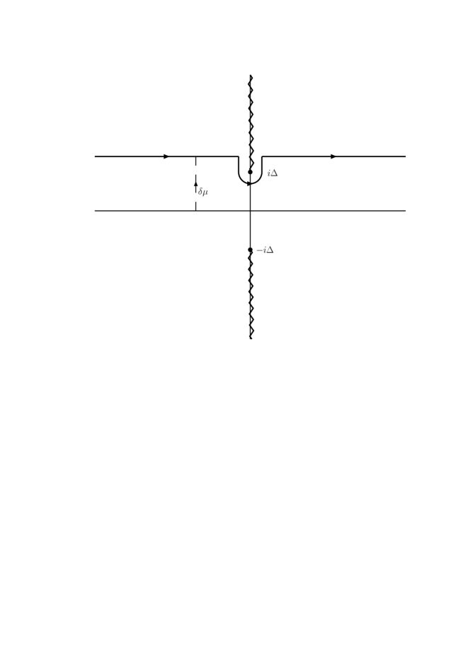
Figure 5: The contour for $z$-integral.

Alternatively, the $z$-integral can be regarded an integral along a contour running from $-\infty+i\delta$ to $\infty+i\delta$ and going around the branch point $i\Delta$ counterclockwisely plus an integral from $i\delta\mu+0^{+}$ to $i\delta\mu-0^{+}$ going around the branch point clockwisely. The contour of the former can be shifted to the real axis, leaving the result independent of $\delta\mu$. We obtain that

$$I(k|\delta\mu)=I(k|0)+I_{1}(k|\delta\mu)$$ (121)

with

$$I(k|0)=\frac{\Delta^{2}}{2\pi}\int_{-1}^{1}dx\int_{-\infty}^{\infty}dz\frac{1}{\sqrt{z^{2}+\Delta^{2}}\Big{(}z^{2}+\Delta^{2}+\frac{1}{4}k^{2}x^{2}\Big{)}}$$ (122)

and

$$I_{1}(k|\delta\mu)=\frac{\Delta^{2}}{2\pi}\int_{-1}^{1}dx\int_{i\delta\mu+0^{+}}^{i\delta\mu-0^{+}}dz\frac{1}{\sqrt{z^{2}+\Delta^{2}}\Big{(}z^{2}+\Delta^{2}+\frac{1}{4}k^{2}x^{2}\Big{)}}.$$ (123)

Using the formula

$$\int d\xi\frac{1}{\sqrt{\xi^{2}+a^{2}}(\xi^{2}+b^{2})}=\frac{1}{2b\sqrt{b^{2}-a^{2}}}\ln\frac{b\sqrt{\xi^{2}+a^{2}}+\sqrt{b^{2}-a^{2}}\xi}{b\sqrt{\xi^{2}+a^{2}}-\sqrt{b^{2}-a^{2}}\xi}$$ (124)

and making the transformation for the $x$-integral, $x=\frac{2\Delta}{k}\sinh\theta$, we end up with

$$I(k|0) = \frac{4\Delta}{\pi k}\int_{0}^{\theta_{c}}d\theta\frac{\theta}{\sinh\theta}$$

$$= \frac{8\Delta}{\pi k}\Big{[}\frac{\pi^{2}}{8}+\frac{1}{2}\theta_{c}\ln\tanh\frac{\theta_{c}}{2}-{\rm Li}_{2}(e^{-\theta_{c}})+\frac{1}{4}{\rm Li}_{2}(e^{-2\theta_{c}})\Big{]}$$

and

$$I_{1}(k|\delta\mu)=\frac{2\Delta}{\pi k}\int_{0}^{\theta_{c}}\frac{d\theta}{\sinh\theta}\ln\frac{|\sqrt{\delta\mu^{2}-\Delta^{2}}\cosh\theta-\delta\mu\sinh\theta|}{\sqrt{\delta\mu^{2}-\Delta^{2}}\cosh\theta+\delta\mu\sinh\theta},$$ (126)

where $\theta_{c}$ is defined by $\sinh\theta_{c}=\frac{k}{2\Delta}$ and ${\rm Li}_{2}(z)$ is Spence function, i.e.

$${\rm Li}_{2}(z)=-\int_{0}^{z}dt\frac{\ln(1-t)}{t}=\sum_{n=1}^{\infty}\frac{z^{n}}{n^{2}}.$$ (127)

The integration of $J(k|\delta\mu)$ can be carried following the same procedure and the result is elementary,

$$J(k|\delta\mu) = \frac{16\Delta^{3}}{\pi k^{3}}(\theta_{c}\cosh\theta_{c}-\sinh\theta_{c})$$

$$+ \frac{8\Delta^{3}}{\pi q^{3}}\Big{[}\cosh\theta_{c}\ln\frac{|\sqrt{\delta\mu^{2}-\Delta^{2}}\cosh\theta_{c}-\delta\mu\sinh\theta_{c}|}{\sqrt{\delta\mu^{2}-\Delta^{2}}\cosh\theta_{c}+\delta\mu\sinh\theta_{c}|}-\frac{\delta\mu}{\Delta}\ln\frac{|\sqrt{\delta\mu^{2}-\Delta^{2}}-\Delta\sinh\theta_{c}|}{\sqrt{\delta\mu^{2}-\Delta^{2}}+\Delta\sinh\theta_{c}}\Big{]}.$$

Upon decomposing $K(k|\delta\mu)$ into $K(k|0)+K_{1}(k|\delta\mu)$ in analog to $I(k|\delta\mu)$ we observe that $K(k|0)=0$ and the integration of $K_{1}(k|\delta\mu)$ yields

$$K_{1}(k|\delta\mu)=\frac{4\Delta}{\pi k}{\rm Re}\Big{[}{\rm Li}_{2}\Big{(}\frac{k}{2\sqrt{\delta\mu^{2}-\Delta^{2}}}\Big{)}-\frac{1}{4}{\rm Li}_{2}\Big{(}\frac{k^{2}}{4(\delta\mu^{2}-\Delta^{2})}\Big{)}\Big{]}.$$ (129)

The small $k$ expansion of $I(k|\delta\mu)$, $J(k|\delta\mu)$ and $K(k|\delta\mu)$ can be obtainede easily from their integral representations as is shown in the text. The large $k$ behavior of $I(k|0)$ and $J(k|\delta\mu)$ cab be extracted readily from their explicit form with $e^{\theta_{c}}>>1$. As to $I_{1}(k|\delta\mu)$, we write

$$\int_{0}^{\theta_{c}}d\theta()=\int_{0}^{\infty}d\theta()-\int_{\theta_{c}}^{\infty}d\theta().$$ (130)

The large $k$ expansion can be carried out with the aid of the formula ( the derivation is outlined at the end of this appendix ).

$$\int_{0}^{\infty}\frac{d\theta}{\sinh\theta}\ln\frac{\sqrt{\delta\mu^{2}-\Delta^{2}}\cosh\theta+\delta\mu\sinh\theta}{|\sqrt{\delta\mu^{2}-\Delta^{2}}\cosh\theta-\delta\mu\sinh\theta|}=\frac{\pi^{2}}{2}$$ (131)

and the expansion of the integrand of the 2nd integral on RHS of (130) according to the powers of $e^{-\theta}$. The large $k$ expansion of $K(k|\delta\mu)$ follows from the formula

$${\rm Re}{\rm Li}_{2}(z)=\frac{\pi^{2}}{3}-\frac{1}{2}\ln^{2}z-{\rm Li}_{2}\Big{(}\frac{1}{z}\Big{)}$$ (132)

for $z>1$. We obtain that

$$I(k|\delta\mu)\simeq\frac{4}{\pi k^{2}}\Big{(}-2\ln\frac{k}{\Delta}-2+\ln\frac{\delta\mu+\sqrt{\delta\mu^{2}-\Delta^{2}}}{\delta\mu-\sqrt{\delta\mu^{2}-\Delta^{2}}}\Big{)},$$ (133)

$$J(k|\delta\mu)\simeq\frac{4}{\pi k^{2}}\Big{(}2\ln\frac{k}{2}-2+\ln\frac{\delta\mu+\sqrt{\delta\mu^{2}-\Delta^{2}}}{\delta\mu-\sqrt{\delta\mu^{2}-\Delta^{2}}}\Big{)}$$ (134)

and

$$K(k|\delta\mu)\simeq\frac{\pi\Delta}{k}.$$ (135)

Finally, let us sketch how the formula (130) can be derived. Introduce a function of $z$,

$$f(z)=\int_{0}^{\infty}\frac{d\theta}{\sinh\theta}\ln\frac{1+z\tanh\theta}{1-z\tanh\theta}$$ (136)

the LHS of (130) equals the real part of its value at $z=\frac{\delta\mu}{\sqrt{\delta\mu^{2}-\Delta^{2}}}$. For $z<1$, the integrand can be expanded according to the powers of $z$ and the integration of the coefficients can be carried out explicitly. The resultant power series can be recognized to be that of $\pi\sin^{-1}z$. The analytic continuation to $z>1$ gives rise to the RHS of (130).

Appendix C Electric charge density induced by Goldstone fields

On writing the electric charge density induced by Goldstone fields

$$\delta\rho(\vec{k})=\sum_{a}\kappa_{a}(k)\phi_{a}(\vec{k}),$$ (137)

we have

$$\kappa_{a}(k)=-\frac{1}{2}eT\sum_{n}\int\frac{d^{2}\vec{p}}{(2\pi)^{3}}{\rm Tr}\gamma_{0}Q{\cal S}_{M}(\omega_{n},\vec{p}+\vec{k})\gamma_{5}G_{a}{\cal S}_{M}(\omega_{n},\vec{p}),$$ (138)

where $Q=\rho_{3}(a+b\tau_{3})$, the matrix $G_{4}=\varepsilon^{1}\rho_{1}$, $G_{5}=\varepsilon^{1}\rho_{2}$, $G_{6}=\varepsilon^{2}\rho_{1}$, $G_{7}=\varepsilon^{2}\rho_{2}$ and $G_{8}=\varepsilon^{3}\rho_{1}$ for the five Goldstone fields.

With respect to r, g, and b color indexes, the propagator assumes the block structure

$${\cal S}_{M}=\left(\begin{array}[]{cc}{\cal S}_{M}^{SU(2)}&0\\ 0&{\cal S}_{M}^{U(1)}\end{array}\right)$$ (139)

while the matrix $\varepsilon^{\rho}$ ($\rho=1,2)$ takes the form

$$\varepsilon^{\rho}=\left(\begin{array}[]{cc}0&\chi_{\rho}(2\times 1)\\ -\chi^{\dagger}(1\times 2)&0\end{array}\right).$$ (140)

Therefore the trace with respect to the group indexes vanishes for $\varepsilon^{1}$ and $\varepsilon^{2}$. Consequently

$$\kappa_{4}(k)=\kappa_{5}(k)=\kappa_{6}(k)=\kappa_{7}(k)=0.$$ (141)

Coming to $\kappa_{8}(k)$, we firstly take the transpose of the matrix under the trace on RHS of (138), then we employ the identity

$$\gamma_{0}C{\cal S}_{M}^{T}(p_{0},\vec{p})C^{\dagger}\gamma_{0}=-{\cal S}_{M}(p_{0},-\vec{p}),$$ (142)

and transform the integration variable from $\vec{p}$ to $-\vec{p}-\vec{k}$. We find

$$\kappa_{8}(k)=-\kappa_{8}(k)=0.$$ (143)

References

- (1) S.C. Frautschi, Asymptotic freedom and color superconductivity in dense quark matter, Proc.of the Workshop on Hadronic Matter at Extreme Energy Density, N. Cabibbo (Editor), Erice, Italy (1978); F. Barrois, Nucl. Phys. B129 (1977),390; D. Bailin and A. Love, Phys. Rep. 107, 325(1984).
- (2) R. Rapp, T. Schäfer, E. V. Shuryak and M. Velkovsky, Phys. Rev. Lett. 81, 53 (1998); M. Alford, K. Rajagopal, and F. Wilczek, Phys. Lett. B 422, 247 (1998).
- (3) K. Rajagopal and F. Wilczek, hep-ph/0011333; D. K. Hong, Acta Phys. Polon. B 32, 1253 (2001); M. Alford, Ann. Rev. Nucl. Part. Sci. 51, 131 (2001); T. Schäfer, hep-ph/0304281; D. H. Rischke, Prog. Part. Nucl. Phys. 52, 197 (2004); M. Buballa, Phys. Rept. 407, 205 (2005); H.-C. Ren, hep-ph/0404074; M. Huang, Int. J. Mod. Phys. E 14, 675 (2005); I. A. Shovkovy, Found. Phys. 35, 1309 (2005).
- (4) M. Alford and K. Rajagopal, JHEP 0206, 031 (2002); A.W. Steiner, S. Reddy and M. Prakash, Phys. Rev. D 66, 094007 (2002). M. Huang, P. F. Zhuang and W. Q. Chao, Phys. Rev. D 67, 065015 (2003).
- (5) I. Shovkovy and M. Huang, Phys. Lett. B 564, 205 (2003); M. Huang and I. Shovkovy, Nucl. Phys. A729, 835 (2003).
- (6) M. Alford, C. Kouvaris and K. Rajagopal, Phys. Rev. Lett. 92, 222001 (2004); Phys. Rev. D 71, 054009 (2005).
- (7) M. Huang and I. A. Shovkovy, Phys. Rev. D 70, 051501 (2004); M. Huang and I. A. Shovkovy, Phys. Rev. D 70, 094030 (2004).
- (8) R. Casalbuoni, R. Gatto, M. Mannarelli, G. Nardulli and M. Ruggieri, Phys. Lett. B 605, 362 (2005);
- (9) M. Alford and Q. h. Wang, hep-ph/0501078.
- (10) G. Sarma, J. Phys. Chem. Solids 24, 1029 (1963).
- (11) P. Fulde and R. A. Ferrell, Phys. Rev. 135, A550 (1964); A. I. Larkin and Yu. N. Ovchinnikov, Sov. Phys. JETP 20, 762 (1965).
- (12) H. Muther and A. Sedrakian, Phys. Rev. C 67, 015802 (2003) A. Sedrakian and J. W. Clark,
- (13) W. V. Liu and F. Wilczek, Phys. Rev. Lett. 90, 047002 (2003); E. Gubankova, W.V. Liu and F. Wilczek, Phys. Rev. Lett. 91, 032001 (2003).
- (14) S.-T. Wu and S. Yip, Phys. Rev. A 67, 053603 (2003).
- (15) J. Singleton, J. A. Symington, M.-S. Nam, A. Ardavan, M. Kurmoo, and P. Day, J. Phys.: Condens. Matter 12, L641 (2000); S. Manalo and U. Klein, J. Phys.: Condens. Matter 12, L471 (2000); M. A. Tanatar, T. Ishiguro, H. Tanaka, and H. Kobayashi, Phys. Rev. B 66, 134503 (2002); J. L. O’Brien, H. Nakagawa, A. S. Dzurak, R. G. Clark, B. E. Kane, N. E. Lumpkin, R. P. Starrett, N. Muira, E. E. Mitchell, J. D. Goettee, D. G. Rickel, and J. S. Brooks, Phys. Rev. B 61, 1584 (2000); H. A. Radovan, N. A. Fortune, T. P. Murphy, S. T. Hannahs, E. C. Palm, S. W. Tozer, D. Hall, Nature 425, 51 (2003); A. Bianchi, R. Movshovich, C. Capan, P. G. Pagliuso, and J. L. Sarrao, Phys. Rev. Lett. 91, 187004 (2003).
- (16) K. Yang, cond-mat/0603190.
- (17) D. T. Son and M. A. Stephanov, cond-mat/0507586; L. He, M. Jin and P. Zhuang, cond-mat/0601147. H. Hu, and X.J. Liu, cond-mat/060332; C.-H. Pao, S.-K. Yip, cond-mat/0604530.
- (18) M. W. Zwierlein, A. Schirotzek, C. H. Schunck, and W. Ketterle, Science 311 (5760), 492-496 (2006); G. B. Partridge, W. Li, R. I. Kamar, Y. Liao, and R. G. Hulet, cond-mat/0511752; M.W. Zwierlein, C. H. Schunck, A. Schirotzek, and W. Ketterle, Nature 442, 54-58 (2006) Y. Shin, M. W. Zwierlein, C. H. Schunck, A. Schirotzek, W. Ketterle, Phys. Rev. Lett. 97, 030401 (2006); M. W. Zwierlein, and W. Ketterle, cond-mat/0603489.
- (19) M. G. Alford, J. A. Bowers and K. Rajagopal, Phys. Rev. D 63, 074016 (2001).
- (20) D. K. Hong and Y. J. Sohn, hep-ph/0107003; I. Giannakis, J. T. Liu and H. c. Ren, Phys. Rev. D 66, 031501 (2002); R. Casalbuoni and G. Nardulli, Rev. Mod. Phys. 76, 263 (2004); J. A. Bowers, hep-ph/0305301; K. Rajagopal and R. Sharma, hep-ph/0605316.
- (21) I. Giannakis and H. C. Ren, Phys. Lett. B 611, 137 (2005); I. Giannakis and H. C. Ren, Nucl. Phys. B 723, 255 (2005); I. Giannakis, D. f. Hou and H. C. Ren, Phys. Lett. B 631, 16 (2005).
- (22) D. K. Hong, hep-ph/0506097.
- (23) Mei Huang, Int. J. Mod. Phys. A 21, 910 (2006); Mei Huang, Phys. Rev. D 73, 045007 (2006).
- (24) E. V. Gorbar, M. Hashimoto and V. A. Miransky, Phys. Lett. B 632, 305 (2006).
- (25) M. Hashimoto, hep-ph/0605323.
- (26) A. Kryjevski, hep-ph/0508180; T. Schafer, Phys. Rev. Lett. 96, 012305 (2006); A. Gerhold and T. Schafer, hep-ph/0603257.
- (27) C.H. Pao, Shin-Tza Wu, S.-K. Yip, cond-mat/0506437.
- (28) K. Iida and K. Fukushima, hep-ph/0603179.
- (29) I. Giannakis, DeFu Hou, Mei Huang and Hai-cang Ren, hep-ph/0606178.
- (30) M. G. Alford, K. Rajagopal, S. Reddy and F. Wilczek, Phys. Rev. D 64, 074017 (2001) F. Neumann, M. Buballa, and M. Oertel, Nucl. Phys. A714, 481 (2003); H. Grigorian, D. Blaschke and D. N. Aguilera, Phys. Rev. C 69, 065802 (2004); S. Reddy and G. Rupak, Phys. Rev. C 71, 025201 (2005).
- (31) I. Shovkovy, M. Hanauske and M. Huang, Phys. Rev. D 67, 103004 (2003);
- (32) H. Kleinert, cond-mat/9503030; M.Franz, Z. Tesanovic, Phys.Rev.Lett.87, 257003(2001); M.Franz, Z. Tesanovic, O.Vafek, Phys.Rev.B66(2002), 054535; A. Melikyan, Z. Tesanovic, cond-mat/0408344.
- (33) R. Casalbuoni, Z. y. Duan and F. Sannino, Phys. Rev. D 62, 094004 (2000); V. A. Miransky, I. A. Shovkovy and L. C. R. Wijewardhana, Phys. Rev. D 64, 096002 (2001); D. H. Rischke and I. A. Shovkovy, Phys. Rev. D 66, 054019 (2002).
- (34) I. Giannakis, D. Hou, M. Huang and H. c. Ren, cond-mat/0603263.
- (35) We thank Professor Atiyah for this information.
- (36) S. R. Coleman and E. Weinberg, Phys. Rev. D 7, 1888 (1973); S. R. Coleman, Phys. Rev. D 15, 2929 (1977), [Erratum-ibid. D 16, 1248 (1977)].
- (37) E. J. Weinberg and A. q. Wu, Phys. Rev. D 36, 2474 (1987).
- (38) I. Shovkovy, private communication.