Variational Method for Photon Emission from Quark-Gluon Plasma

Abstract

Variational method has been applied to estimate Landau-Pomeranchuk-Migdal (LPM) effects on virtual photon emission from the quark gluon plasma as a function of photon mass. The variational method was well tested for the LPM effects in real photon emission. For virtual photons, LPM effects arising from multiple scatterings of quarks in the plasma are determined by the integral equations for the transverse vector function (${\bf\tilde{f}(\tilde{p}_{\perp})}$) and the longitudinal function ($\tilde{g}({\bf\tilde{p}_{\perp}})$). We extended the variational method to solve these transverse and longitudinal equations for a variable set {$p_{0},q_{0},Q^{2}$}, considering bremsstrahlung and $\bf aws$ processes. We solved these equations, also by the self consistent iterations for comparing with the results of variational method. In order to estimate the variational parameter, we obtained empirical fits for the peak positions of the ${\bf p_{\perp}\cdot\tilde{f}(\tilde{p}_{\perp})}$, $p_{\perp}\tilde{g}({\bf\tilde{p}_{\perp}})$ distributions from iteration method. We propose that the optimized variational parameter for virtual photon emission is approximately equal to these empirical peak position values. The detailed study showed that the variational method gives reliable results for LPM effects on virtual photon emission for photon virtuality of the order $Q^{2}/T^{2}\leq 100$. At low $Q^{2}$, the peak positions for $\tilde{p}_{\perp}$ distributions of transverse vector functions for virtual photons nearly coincide with the peak positions of corresponding distributions of real photons. We calculated imaginary part of photon retarded polarization tensor as a function of $Q^{2}/T^{2}$ using empirical variational parameters.

Study of the physical processes in quark matter as compared to that in hadronic matter plays a crucial role for identifying the Quark gluon plasma (QGP) state, expected to be formed in the relativistic heavy ion collisions. In this context, electromagnetic processes such as photons and dilepton emission are important as signals peitz ; gale ; rapp to identify this de-confined state. In depth study of photon emission processes in quark-gluon plasma were presented kapusta ; bair . In the hard thermal loops braaten (HTL) effective theory, Compton scattering and quark-antiquark annihilation processes contribute at one loop level to photon emission in quark matter. At the two loop level, the processes of bremsstrahlung brem and a crossed process of annihilation with scattering called ${\bf aws}$ bremaws ; ktkl contribute to photon emission. Importantly, these two loop processes contribute at the leading order $O(\alpha\alpha_{s})$ resulting from a special effect called the collinear singularity that is regularized by the effective thermal masses. Owing to the same reasons, higher loop multiple scatterings having a ladder topology also contribute at the same order arnold1 ; arnold2 giving a decoherent correction to the two loop processes. These rescatterings have been resummed arnold1 ; arnold2 , effectively implementing the Landau-Pomeranchuk-Migdal (LPM) effects landau1 ; landau2 ; migdal . LPM effects arise due to rescattering of quarks in the medium during photon formation time. The rescattering corrections strongly modify the two loop contributions for bremsstrahlung and $\bf aws$ processes for real photon emission arnold1 ; arnold2 .

Photon production rates from bremsstrahlung and $\bf aws$ processes including the LPM effects are estimated by using Eq.1 in terms of a transverse vector function ${\bf\tilde{p}_{\perp}\cdot\Re\tilde{f}(\tilde{p}_{\perp})}$ arnold2 . The resummation of multiple scatterings leads to the AMY integral equation for the transverse vector function for real photons, given in Eq.2 arnold2 .

$${\cal R}_{b,a} = \frac{80\pi T^{3}\alpha\alpha_{s}}{(2\pi)^{3}9\kappa}\int dp_{0}\left[\frac{p_{0}^{2}+(p_{0}+q_{0})^{2})}{p_{0}^{2}(p_{0}+q_{0})^{2})}\right]\times$$ (1)

$$\left[n_{f}(q_{0}+p_{0})(1-n_{f}(p_{0}))\right]\times$$

$$~{}\int\frac{\bf d^{2}\tilde{p}_{\perp}}{(2\pi)^{2}}2{\bf\tilde{p}_{\perp}\cdot\Re\tilde{f}(\tilde{p}_{\perp})}$$

$$2{\bf\tilde{p}_{\perp}} = i\delta\tilde{E}({\bf\tilde{p}_{\perp}}){\bf\tilde{f}}({\bf\tilde{p}_{\perp}})+$$ (2)

$$\int\frac{d^{2}{\bf\tilde{\ell}_{\perp}}}{(2\pi)^{2}}\tilde{C}({\bf\tilde{\ell}_{\perp}})\left[{\bf\tilde{f}}({\bf\tilde{p}_{\perp}})-{\bf\tilde{f}}({\bf\tilde{p}_{\perp}+\tilde{\ell}_{\perp}})\right]$$

$$\delta\tilde{E}({\bf\tilde{p}_{\perp}}) = \frac{q_{0}T}{2p_{0}(q_{0}+p_{0})}\left[\tilde{p}_{\perp}^{2}+\kappa\right]$$ (3)

$${\cal R}_{b,a} = {\cal C}_{k}\int dp_{0}\left[p_{0}^{2}+(p_{0}+q_{0})^{2})\right]\left[n_{f}(q_{0}+p_{0})\right.$$ (4)

$$\left.(1-n_{f}(p_{0}))\right]C_{g}g(x)$$

$$g(x) = g(p_{0},q_{0},T)$$

$$x = \frac{1}{\kappa_{0}}\frac{q_{0}T}{p_{0}(p_{0}+q_{0})}$$ (5)

$${\cal C}_{k} = \frac{40\alpha\alpha_{s}T}{9\pi^{4}q_{0}^{2}}$$ (6)

$$\kappa_{0} = \frac{M_{\infty}^{2}}{m_{D}^{2}}\approx\frac{1}{4}~{}\mbox{and}~{}C_{g}=\frac{\kappa_{0}}{T}$$ (7)

The function $\Re{\bf\tilde{f}(\tilde{p}_{\perp})}$ in Eq.1, which consists of the LPM effects, can be taken as transverse momentum vector ${\bf(\tilde{p}_{\perp})}$ times a scalar function of transverse momentum ${\tilde{p}_{\perp}}$. The tilde sign  $\tilde{}$  represents dimensionless quantities in units of Debye mass $m_{D}$ as defined in arnold2 . The function ${\bf\tilde{p}_{\perp}\cdot\Re\tilde{f}(\tilde{p}_{\perp})}$ is determined by the AMY equation (Eq.2) in terms of energy denominator $\tilde{\delta E}$ given in Eq.3 and the collision kernel ($\tilde{C}({\bf\tilde{\ell}_{\perp}})$). We reported that the complex LPM effects can be very well reproduced by introducing the photon emission function $g(x)$ defined in Eq.4, of a dynamical variable $x$ defined in Eq.5 svsprc . In terms of a single variable function $g(x)$, the photon emission rates are estimated using Eqs.4-7 for any quark momentum, photon energy and plasma temperature.

I Variational Method for Emission of Real Photons

AMY integral equation consisting of LPM effects was solved using the variational approach and the photon emission rates were reported in arnold2 . In the present work, we follow this variational method and expand the real and imaginary parts of ${\bf\tilde{f}(\tilde{p}_{\perp})}$ in terms of a basis set $\{\phi_{j}\}$ of trial functions as shown in Eqs.8-11. The dimensions of the spaces for real and imaginary parts are $N_{r}$ and $N_{i}$. The energy function $\tilde{\delta E}_{mn}$ and the quantities $\tilde{S}_{m,T}$ are calculated by the overlap integrals with the basis trial functions as shown in Eqs.I,13. The overlap integrals $\tilde{C}^{r}_{mn}$ that involve the collision kernels are shown in Eq.14. Another quantity $\tilde{C}^{i}_{mn}$ involving imaginary part is similar to $\tilde{C}^{r}_{mn}$.

$$\Re{\bf\tilde{f}(\tilde{p}}_{\perp}) = {\bf\tilde{p}}_{\perp}\sum_{j=1}^{N_{r}}a_{j,T}\phi_{j}^{r}(\tilde{p}_{\perp}^{2})$$ (8)

$$\Im{\bf\tilde{f}(\tilde{p}}_{\perp}) = {\bf\tilde{p}}_{\perp}\sum_{j=1}^{N_{i}}b_{j,T}\phi_{j}^{i}(\tilde{p}_{\perp}^{2})$$ (9)

$$\phi_{j}^{r}(\tilde{p}_{\perp}^{2}) = \frac{(\tilde{p}_{\perp}^{2}/A)^{j-1}}{(1+(\tilde{p}_{\perp}^{2}/A)^{N_{r}+2}},~{}~{}~{}~{}j=1,...,N_{r}$$ (10)

$$\phi_{j}^{i}(\tilde{p}_{\perp}^{2}) = \frac{(\tilde{p}_{\perp}^{2}/A)^{j-1}}{(1+(\tilde{p}_{\perp}^{2}/A)^{N_{i}}},~{}~{}~{}~{}~{}~{}j=1,...,N_{i}$$ (11)

$$\tilde{\delta E}_{mn} = \left(\phi_{m}^{r},{\tilde{\delta E}}\phi_{n}^{i}\right)$$

$$= \int\frac{d^{2}{\bf{\tilde{p}}}_{\perp}}{(2\pi)^{2}}\phi_{m}^{r}({\bf{\tilde{p}}}_{\perp}){\tilde{\delta E}}\phi_{n}^{i}({\bf{\tilde{p}}}_{\perp})$$

$$\tilde{S}_{m,T} = \left(2{\bf{\tilde{p}}}_{\perp},{\bf{\tilde{p}}}_{\perp}\phi_{m}^{r}\right)$$ (13)

$$\tilde{C}^{r}_{mn} = \frac{1}{2}\int\frac{d^{2}{\bf\tilde{p}}_{\perp}}{(2\pi)^{2}}\frac{d^{2}{\bf\tilde{q}}_{\perp}}{(2\pi)^{2}}\tilde{C}({\bf\tilde{q}}_{\perp})\left[{\bf\tilde{p}}_{\perp}\phi_{m}^{r}({\bf\tilde{p}}^{2})\right.$$ (14)

$$-\left.({\bf\tilde{p}}_{\perp}+{\bf\tilde{q}}_{\perp})\phi_{m}^{r}(|{\bf\tilde{p}}_{\perp}+{\bf\tilde{q}}_{\perp}|^{2})\right]\cdot\left[{\bf\tilde{p}}_{\perp}\phi_{n}^{r}({\bf\tilde{p}}^{2})\right.$$

$$-\left.({\bf\tilde{p}}_{\perp}+{\bf\tilde{q}}_{\perp})\phi_{n}^{r}(|{\bf\tilde{p}}_{\perp}+{\bf\tilde{q}}_{\perp}|^{2})\right]$$

$a_{j,T},b_{j,T}$ in the Eqs.8,9 are the expansion coefficients for real and imaginary parts of ${\bf\tilde{f}(\tilde{p}}_{\perp})$ respectively. Here, the subscripts T and also in $\tilde{S}_{m,T}$ represent transverse vector function ${\bf\tilde{f}}{\bf(\tilde{p}_{\perp})}$. Using the trial functions, some of these quantities can be evaluated analytically or simplified as shown in Eqs.15-19. The choice of dimensions for real and imaginary parts should be pragmatically large enough for performing calculations. For real photon emission calculations, we used two flavors, three colors, $\alpha_{s}$=0.20 and $N_{r}=N_{i}=8$. A few cases were verified for convergence using $N_{r}=N_{i}$=10 and 12. These results for photon emission rates were reported earlier svsprc . However, it is instructive to present the details of variational calculations and analysis of results for the case of real photons.

$$\tilde{\delta E}_{m,n,T} = \frac{q_{0}TA^{2}}{2p_{0}r_{0}}K_{T}$$ (15)

$$K_{T} = AK(m+n,N)+\kappa K(m+n-1,N)$$

$$\tilde{S}_{m,T} = 2A^{2}K(m,N_{r})$$ (16)

$$K(m,n) = \frac{m!(N-m)!}{4\pi(N+1)!}$$ (17)

$$N = N_{r}+N_{i}$$ (18)

$$\tilde{C}^{r}_{mn} = \frac{1}{32\pi^{2}}\int d\tilde{p}_{\perp}^{2}d\tilde{q}_{\perp}^{2}\int_{-\pi}^{\pi}\frac{d\theta}{2\pi}\tilde{C}(\tilde{q}_{\perp})$$ (19)

$$\left\{\tilde{p}_{\perp}^{2}\phi_{m}^{r}(\tilde{p}_{\perp}^{2})\phi_{n}^{r}(\tilde{p}_{\perp}^{2})+\right.$$

$$|\tilde{\bf{p}}_{\perp}+\tilde{\bf{q}}_{\perp}|^{2}\phi_{m}^{r}(|\tilde{\bf p}_{\perp}+\tilde{\bf q}_{\perp}|^{2})\phi_{n}^{r}(|\tilde{\bf p}_{\perp}+\tilde{\bf q}_{\perp}|^{2})$$

$$-\left(\tilde{p}_{\perp}^{2}+\tilde{p}_{\perp}\tilde{q}_{\perp}\cos\theta\right)\left[\phi_{m}^{r}(|\tilde{\bf p}_{\perp}+\tilde{\bf q}_{\perp}|^{2})\phi_{n}^{r}(\tilde{p}_{\perp}^{2})\right.$$

$$\left.\left.+(m\leftrightarrow n)\right]\right\}$$

In the variational approach, the trial functions consist of a variational parameter $A$ which needs to be optimized to obtain correct results. The ${\bf\tilde{p}_{\perp}\cdot\Re\tilde{f}(\tilde{p}_{\perp})}$ distributions are usually sharply peaked and therefore the optimized value of the variational parameter $A_{v}(A=A_{v}^{2})$ should be around the peak positions of these distributions. In our earlier paper, we simplified this variational approach and extended this method to finite baryon density case svs1 . It was shown that the variational parameter can be taken as $A=A_{v}^{2}(p_{0},q_{0},T)$, together with $A_{v}(p_{0},q_{0})=\left|{p_{0}(q_{0}+p_{0})}/{q_{0}}\right|^{0.31}$ and constraint $A_{v}\geq 0.31$. In the calculations that follow, we used this empirical result for the variational parameter. In order to test the empirical values of the variational parameter, we transform the inner product integral ${\bf\tilde{p}_{\perp}\cdot\Re\tilde{f}(\tilde{p}_{\perp})}$ defined over [0,$\infty$] to a finite interval of [0,1] by defining a variable $y$ in Eq.20 (see arnold2 ). In terms of $y$, this inner product is given in Eq.21. Then we estimate the value of ${\tilde{p}_{\perp}}$ where the integrand in Eq.21 peaks. If the value of the variational parameter $A(=A_{v}^{2})$ used is correct, the result should be $y=\frac{1}{2}$ at this peak position ${\tilde{p}_{\perp}}$. Therefore, finding the optimized value of the variational parameter is equivalent to finding the peak positions of these ${\bf\tilde{p}_{\perp}\cdot\Re\tilde{f}(\tilde{p}_{\perp})}$ distributions.

$$y = \frac{|{\bf\tilde{p}}_{\perp}|}{A^{1/2}+|{\bf\tilde{p}}_{\perp}|}.$$ (20)

$$\left({\bf\tilde{p}}_{\perp},{\bf\tilde{f}}\right) = \frac{1}{\pi}\int_{0}^{1}\frac{A^{2}y^{3}}{(1-y)^{5}}\chi\left(Ay^{3}/(1-y)^{2}\right)dy.$$ (21)

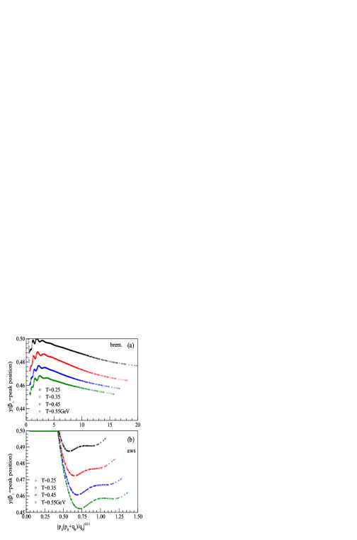
Figure 1: The $y$ function constructed from the peak positions of real photon ${\bf\tilde{p}_{\perp}}\cdot\Re{\bf\tilde{f}(\tilde{p}_{\perp})}$ distributions. Symbols represent the peak positions of ${\bf p_{\perp}}$ distributions from variational method for different $\{p_{0},q_{0},T\}$ values. The variational method used an empirical formula for variational parameter. The $y$ value should be 1/2 for truly optimized variational parameter. Figure shows that the empirical variational parameter values used for real photons satisfied this constraint approximately.

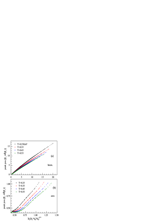
Figure 2: The peak positions of real photon ${\bf\tilde{p}_{\perp}}\cdot\Re{\bf\tilde{f}(\tilde{p}_{\perp})}$ distributions versus (peak positions from) empirical formula. Symbols represent the peak positions from variational method for different $\{p_{0},q_{0},T\}$ values.

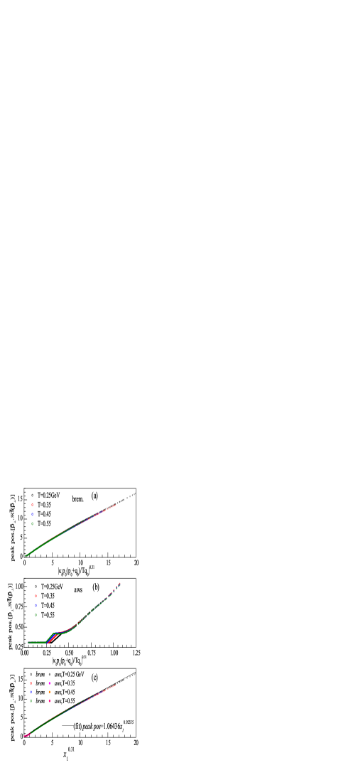
Figure 3: The peak positions of real photon ${\bf\tilde{p}_{\perp}}\cdot\Re{\bf\tilde{f}(\tilde{p}_{\perp})}$ distributions versus (peak positions from) empirical formula values, for (a) bremsstrahlung and for (b) ${\bf aws}$. Symbols represent the peak positions of ${\bf p_{\perp}}$ distributions from variational method for different $\{p_{0},q_{0},T\}$ values. Figure shows that the $x_{1}$ variable defined in text (Eq.43) for real photons is a good scale. The data of (a) and (b) are all plotted in figure (c). The empirical fit function and its parameters are shown in figure (c) which can be used to fix the optimized variational parameter.

We observed that these distributions are not very sensitive to the exact value of the $A_{v}$ parameter provided the dimension is sufficiently high. Figure. 1 shows $y$ at the peak positions of these ${\bf\tilde{p}_{\perp}\cdot\Re\tilde{f}(\tilde{p}_{\perp})}$ distributions. Figure. 1(a) shows $y$ for bremsstrahlung and 1(b) for ${\bf aws}$ processes, as a function of $\left|{p_{0}(q_{0}+p_{0})}/{q_{0}}\right|^{0.31}$. The figure includes variational calculations for a set of 2304 values of $\{p_{0},q_{0},T\}$ (=24x24x4 values i.e., 24 for $p_{0}$, 24 for $q_{0}$ and 4 temperatures). It can be seen that the $y$ value is close to $\frac{1}{2}$ for both bremsstrahlung and aws processes. However deviation of $y$ from 1/2 increases with increasing temperature, as temperature dependence for variational parameter was not considered. The exact peak position values of these distributions are shown in Figure.2(a) for bremsstrahlung and 2(b) for ${\bf aws}$ processes, as a function of $\left|{p_{0}(q_{0}+p_{0})}/{q_{0}}\right|^{0.31}$. As shown in figure, the peak positions are linear and the temperature dependence is not very strong. However, when these peak positions are plotted versus $x_{1}^{0.31}$ with $x_{1}=\left|\kappa_{0}p_{0}(q_{0}+p_{0})/(Tq_{0})\right|$, all the 2304 points of $\{p_{0},q_{0},T\}$ merge for bremsstrahlung process and similarly for ${\bf aws}$ process as shown in Figs.3(a,b). Further, when the bremsstrahlung and aws peak positions are both together plotted versus $x_{1}^{0.31}$, all the data points of Fig.3(a,b) overlap as shown in Fig.3(c). Therefore, the peak positions of these two processes follow scaling with $x_{1}$ variable. This is not surprising because we have shown earlier that $x_{1}$ is an exact dynamical scale for real photonssvsprc . We have fitted the data by a suitable function and the parameters are shown in Fig.3(c). Therefore for real photon emission, the optimized variational parameter is approximately given by the empirical fit values shown in Fig.3(c) for any temperature, quark momentum and photon energy values.

II Variational Method for virtual Photon emission

Processes that contribute to virtual photon emission in QGP at $\alpha\alpha_{s}$ order alther and the higher order corrections thoma were reported. The HTL one loop processes $q\bar{q}\rightarrow g\gamma^{*}$, and $qg\rightarrow q\gamma^{*}$ contribute to photon polarization tensor at the order $\alpha\alpha_{s}$. Photon emission from QGP as a function of photon mass considering LPM effects was also reported lpmdilep . It was shown that the multiple scatterings modify the imaginary part of self energy as a function of photon energy and momentum both, especially modifying the tree level threshold, $Q^{2}=4M_{\infty}^{2}$ lpmdilep . The dilepton emission rates are estimated in terms of the imaginary part of retarded photon polarization tensor for virtual photons, given by lpmdilep .

$$\frac{dN_{\ell^{+}\ell^{-}}}{d^{4}xd^{4}Q}=\frac{\alpha_{EM}}{12\pi^{4}Q^{2}(e^{q0/T}-1)}\Im\Pi_{R\mu}^{\mu}(Q)$$ (22)

$\Im\Pi_{R\mu}^{\mu}(Q)$ is determined by transverse and longitudinal functions represented by ${\bf f(p_{\perp})},g(p_{\perp})$ resulting from two integral equations. For the case of virtual photon emission, the transverse vector function is determined by the Eq.23 and the energy transfer $\delta{E}(({\bf{p}_{\perp}},p_{0},q_{0},Q^{2})$ lpmdilep . For virtual photons, the coupling of quarks to longitudinal mode must be considered. This results in a scalar function of ${\bf p_{\perp}}$ which is determined by the AGMZ integral equation given in Eq.24 with the collision kernel from kernel . For the case of massive photon emission, this energy denominator $\delta{E}$ is modified from that of real photons by replacing $M_{\infty}^{2}\rightarrow M_{\mbox{eff}}=M_{\infty}^{2}+\frac{Q^{2}}{q_{0}^{2}}{p_{0}r_{0}}$ as in Eq.25. For $Q^{2}>4M_{\infty}^{2}$, this M${}_{\mbox{eff}}$ can vanish or even become negative. $\delta{E}$ energy denominator can be interpreted as inverse formation time of the photon, which acquires dependence on photon mass in addition to the dependence on photon energy, quark momentum of a real photon.

$$2{\bf{p}_{\perp}} = i\delta{E}({\bf{p}_{\perp}},p_{0},q_{0},Q^{2}){\bf{f}}({\bf{p}_{\perp}})+g^{2}C_{F}T$$ (23)

$$\int\frac{d^{2}{\bf{\ell}_{\perp}}}{(2\pi)^{2}}{C}({\bf{\ell}_{\perp}})\left[{\bf{f}}({\bf{p}_{\perp}})-{\bf{f}}({\bf{p}_{\perp}+{\bf\ell}_{\perp}})\right]$$

$$2{\bf\sqrt{|p_{0}r_{0}|}} = i\delta{E}({\bf{p}_{\perp}},p_{0},q_{0},Q^{2})g({\bf{p}_{\perp}})+g^{2}C_{F}T$$ (24)

$$\int\frac{d^{2}{\bf{\bf\ell}_{\perp}}}{(2\pi)^{2}}C({\bf{\ell}_{\perp}})\left[g({\bf{p}_{\perp}})-g({\bf{p}_{\perp}+\bf{\ell}_{\perp}})\right]~{}~{}~{}~{}~{}$$

$$\delta E({\bf{p}_{\perp}},p_{0},q_{0},Q^{2}) = \frac{q_{0}}{2p_{0}r_{0}}\left[{\bf{p}_{\perp}^{2}}+M_{\mbox{eff}}^{2}\right]$$ (25)

In above equations, $r_{0}=p_{0}+q_{0}$ and ${\bf{f}},g$ are actually functions of $p_{0},q_{0},Q^{2}$ represented as, ${\bf{f}}({\bf{p}_{\perp}},p_{0},q_{0},Q^{2})$, $g({\bf{p}_{\perp}},p_{0},q_{0},Q^{2})$. Eq.23 and Eq.2 are identical except for $\delta E$ energy factor. Further, Eq.23 and the Eq.24 are similar on the right side of the equations, however the left side of AGMZ equation is a constant $\sqrt{|p_{0}r_{0}|}$. Aurenche et. al., solved these equations, based on a method of impact parameter representation lpmdilep . As shown in previous section, we have solved the AMY equation for real photons by the variational method and a new method called iterations method by formulating these equations in terms of tilded variables. Therefore, we will transform the two above equations Eqs.23,24 to tilded quantities, and for details see arnold2 ; gef . The transformation for ${\bf p_{\perp},f(p_{\perp})},\delta E({\bf p_{\perp}}),C({\bf p_{\perp}})$ are given by Eq.26.

$${\bf\tilde{p}_{\perp}} = \frac{\bf p_{\perp}}{m_{D}}~{}~{};~{}~{}{\bf\tilde{f}(\tilde{p}_{\perp})}=\frac{m_{D}}{T}{\bf{f}({p}_{\perp})}$$

$${\tilde{\delta E}}({\bf\tilde{p}_{\perp}}) = \frac{T}{m_{D}^{2}}{\delta E(\bf{p}_{\perp}})~{}~{};~{}~{}\tilde{C}{\bf(\tilde{\bf\ell}_{\perp}})=TC({\bf\ell_{\perp}}).$$ (26)

$$2{\bf\tilde{p}_{\perp}} = i\delta\tilde{E}({\bf\tilde{p}_{\perp}},p_{0},q_{0},Q^{2}){\bf\tilde{f}}({\bf\tilde{p}_{\perp}})$$ (27)

$$+\int\frac{d^{2}{\bf\tilde{\bf\ell}_{\perp}}}{(2\pi)^{2}}\tilde{C}({\bf\tilde{\ell}_{\perp}})\left[{\bf\tilde{f}}({\bf\tilde{p}_{\perp}})-{\bf\tilde{f}}({\bf\tilde{p}_{\perp}+\tilde{\bf\ell}_{\perp}})\right]$$

$$\delta\tilde{E}({\bf\tilde{p}_{\perp}},p_{0},q_{0},Q^{2})=\frac{q_{0}T}{2p_{0}(q_{0}+p_{0})}\left[\tilde{p}_{\perp}^{2}+\kappa_{\mbox{\small{eff}}}\right]$$ (28)

In above $\kappa_{\small{\mbox{eff}}}=\frac{M^{2}_{\mbox{\small{eff}}}}{m_{D}^{2}}$. We will divide the above Eq.24, by $m_{D}$ in order to get the following equation, where absorbing 1/$m_{D}$ factor, $g$ is now re-defined. The equation for the longitudinal part could be written as,

$$2\sqrt{\frac{|p_{0}r_{0}|}{m_{D}^{2}}} = i\delta\tilde{E}({\bf\tilde{p}_{\perp}},p_{0},q_{0},Q^{2}){\tilde{g}}({\bf\tilde{p}_{\perp}})+$$ (29)

$$\int\frac{d^{2}{\bf\tilde{\ell}_{\perp}}}{(2\pi)^{2}}\tilde{C}({\bf\tilde{\ell}_{\perp}})\left[{\tilde{g}}({\bf\tilde{p}_{\perp}})-{\tilde{g}}({\bf\tilde{p}_{\perp}+\tilde{\bf\ell}_{\perp}})\right]~{}~{}~{}~{}~{}$$

In the above equation, $g$ transforms as $\tilde{g}({\bf\tilde{p}_{\perp}})=\frac{m_{D}}{T}g({\bf p_{\perp}})$, similar to $\bf f(p_{\perp})$ function. It implies that the $\tilde{g}$ is larger than $g$ by a factor $m_{D}$. Therefore, when the solution for this Eq.29 is obtained and integrated over $\int\frac{d^{2}\bf\tilde{p}_{\perp}}{(2\pi)^{2}}\Re{\tilde{g}{\bf(\tilde{p}_{\perp})}}$, the result will be larger than the true result from Eq.24 by exactly $m_{D}$ factor gef . In the present work, we have solved the above Eq.29 by iterations and variational method with an aim to test the validity of the variational method for a virtual photon case. The variational method for longitudinal part has been re-derived as shown in Eqs.30-41 svssymp . The basis for expansion of the ${\bf\tilde{f}(\tilde{p}}_{\perp})$ is same as in Eqs.8-11. The equations for $\tilde{\delta E}_{mn}$ and $\tilde{S}_{m,T}$ remain same as in Eqs.15,16 except for the change $\kappa\rightarrow\kappa_{\mbox{eff}}$.

$$\Re{\tilde{g}(\bf\tilde{p}}_{\perp}) = \sum_{j=1}^{N_{r}}a_{j,L}\phi_{j}^{r}(\tilde{p}_{\perp}^{2})$$ (30)

$$\Im{\tilde{g}(\bf\tilde{p}}_{\perp}) = \sum_{j=1}^{N_{i}}b_{j,L}\phi_{j}^{i}(\tilde{p}_{\perp}^{2})$$ (31)

$$\phi_{j}^{r}(\tilde{p}_{\perp}^{2}) = \frac{(\tilde{p}_{\perp}^{2}/A)^{j-1}}{(1+\tilde{p}_{\perp}^{2}/A)^{N_{r}+2}},~{}~{}~{}~{}j=1,...,N_{r}$$ (32)

$$\phi_{j}^{i}(\tilde{p}_{\perp}^{2}) = \frac{(\tilde{p}_{\perp}^{2}/A)^{j-1}}{(1+\tilde{p}_{\perp}^{2}/A)^{N_{i}}},~{}~{}~{}~{}~{}~{}~{}~{}j=1,...,N_{i}$$ (33)

$$\tilde{\delta E}_{mn} = \left(\phi_{m}^{r},{\tilde{\delta E}}\phi_{n}^{i}\right)$$

$$= \int\frac{d^{2}{\bf{\tilde{p}}}_{\perp}}{(2\pi)^{2}}\phi_{m}^{r}({\bf{\tilde{p}}}_{\perp}){\tilde{\delta E}}\phi_{n}^{i}({\bf{\tilde{p}}}_{\perp})$$

$$\tilde{\delta E}_{mn,L} = \frac{kTA}{2p_{0}r_{0}}K_{L}$$ (35)

$$K_{L} = AK(m+n-1,N)+\kappa_{\small{\mbox{eff}}}K(m+n-2,N)$$

$$\tilde{S}_{m,T} = \left(2{\bf{\tilde{p}}}_{\perp},{\bf{\tilde{p}}}_{\perp}\phi_{m}^{r}\right)$$ (36)

$$= 2A^{2}K(m,N_{r})$$ (37)

$$\tilde{S}_{m,L} = \left(2\sqrt{\frac{p_{0}r_{0}}{m_{D}^{2}}},\phi_{m}^{r}\right)$$ (38)

$$= \sqrt{\frac{p_{0}r_{0}}{m_{D}^{2}}}K(m-1,N_{r})$$ (39)

$$\tilde{C}^{r}_{mn,L} = \frac{1}{2}\int\frac{d^{2}{\bf\tilde{p}}_{\perp}}{(2\pi)^{2}}\frac{d^{2}{\bf\tilde{q}}_{\perp}}{(2\pi)^{2}}\tilde{C}({\bf\tilde{q}}_{\perp})\left[\phi_{m}^{r}({\bf\tilde{p}}^{2})\right.$$ (40)

$$-\left.\phi_{m}^{r}(|{\bf\tilde{p}}_{\perp}+{\bf\tilde{q}}_{\perp}|^{2})\right]\cdot\left[\phi_{n}^{r}({\bf\tilde{p}}^{2})\right.$$

$$-\left.\phi_{n}^{r}(|{\bf\tilde{p}}_{\perp}+{\bf\tilde{q}}_{\perp}|^{2})\right]$$

$$K(m,n) = \frac{m!(N-m)!}{4\pi(N+1)!}$$

$$\tilde{C}^{r}_{mn} = \frac{1}{32\pi^{2}}\int d\tilde{p}_{\perp}^{2}d\tilde{q}_{\perp}^{2}\int_{-\pi}^{\pi}\frac{d\theta}{2\pi}\tilde{C}(\tilde{q}_{\perp})\left\{\phi_{m}^{r}(\tilde{p}_{\perp}^{2})\phi_{n}^{r}(\tilde{p}_{\perp}^{2})\right.$$ (41)

$$+\phi_{m}^{r}(|\tilde{\bf p}_{\perp}+\tilde{\bf q}_{\perp}|^{2})\phi_{n}^{r}(|\tilde{\bf p}_{\perp}+\tilde{\bf q}_{\perp}|^{2})$$

$$-\left[\phi_{m}^{r}(|\tilde{\bf p}_{\perp}+\tilde{\bf q}_{\perp}|^{2})\phi_{n}^{r}(\tilde{p}_{\perp}^{2})\right.$$

$$\left.\left.+(m\leftrightarrow n)\right]\right\}$$

The equations for expansion of $\tilde{g}({\bf\tilde{p}}_{\perp})$ and the basis functions are similar to transverse part and the equations are given in Eqs.30-33. The energy denominator and other quantities are shown in Eqs.II-41. It is important to note that the variational parameter   $A$   in Eqs.30-41 is in general different for transverse and longitudinal parts. Use of same symbol is misleading and further, the variational parameters for these two parts need to be optimized independently. This is because, in addition to overall $p^{2}_{\perp}$ factor difference in ${\bf\tilde{p}_{\perp}}\cdot\Re{\bf\tilde{f}(\tilde{p}_{\perp})}$,  $\Re\tilde{g}(\tilde{\bf p}_{\perp})$, the equations differ also in the interference terms in Eqs.19,41. In all the calculations that follow, we have used two flavors, three colors, $\alpha_{s}$=0.30, $N_{r}=N_{i}=10$. and T=1.0GeV. Following the iterations and variational methods, we obtained the $\bf p_{\perp}$ distributions for the bremsstrahlung and aws cases for both transverse and longitudinal components. We obtained 350 distributions (5 for $q_{0}$, 10 for $Q^{2}$ and 7 for $p_{0}$ values) for transverse and 350 distributions for longitudinal parts of bremsstrahlung. Similarly the distributions were obtained for aws case. All these distributions were generated in iterations method and many of the cases also by variational method. The results of these two methods were compared. The variational parameter has been varied to optimize the distributions. It was observed that for a given $q_{0}$, the variational method does not give satisfactory results for increasing $Q^{2}$ values and further variational distributions showed large oscillations. However, when the $Q^{2}$ is low, the agreement of results from variational and iterations methods is very good. Therefore, variational method can be used for low $Q^{2}$ values very reliably. The iterations gave correct converging results for all $q_{0},Q^{2}$ values studied. Therefore in the present work, the iterations method is taken as reference standard for these $\bf p_{\perp}$ distributions. These details will be presented in the next section.

III Empirical Analysis of the Solutions of AMY, AGMZ integral equations

Figure 4 shows the ${\bf p_{\perp}}$ distributions for ${\bf\tilde{p}_{\perp}}\cdot\Re{\bf\tilde{f}(\tilde{p}_{\perp})}$ (transverse part of) bremsstrahlung process for five values of $q_{0}=50,30,20,10,5$ GeV. For each $q_{0}$, we have shown distributions (in different colors in figure) for two different photon and quark momenta $(Q^{2},p_{0})$ values. The symbols represent results from iterations method and the curves from the variational method. In many cases, the curves are not visible as the symbols are overwritten on curves, suggesting that the agreement is very good. However, as the $Q^{2}$ increases, these distributions from the variational method show oscillations and deviate from the iterations method. The agreement of variational results with iterations is good for all cases of $Q^{2}$ less than the higher $Q^{2}$ shown in the figures. For example, in the Figure 4, the deviation increases for any $Q^{2}\geq(50^{2}-47^{2})GeV^{2}$ for $q_{0}=50$GeV  ;  $Q^{2}\geq(30^{2}-27^{2})GeV^{2}$ for $q_{0}=30$GeV  ;  $Q^{2}\geq(20^{2}-17^{2})GeV^{2}$ for $q_{0}=20$GeV  ;  $Q^{2}\geq(10^{2}-5^{2})GeV^{2}$ for $q_{0}=10$GeV  ;  $Q^{2}\geq(5^{2}-1^{2})GeV^{2}$ for $q_{0}=5$GeV ;

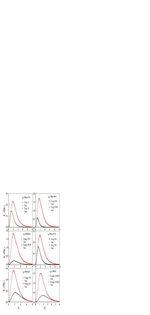
Figure 4: The ${\bf p_{\perp}}$ distributions ${\bf\tilde{p}_{\perp}}\cdot\Re{\bf\tilde{f}(\tilde{p}_{\perp})}$ for transverse part of bremsstrahlung photon emission. The symbols represent results of iterations. About 350 cases of $\{p_{0},q_{0},Q^{2}\}$ values were studied and some are shown in the figure and see text for details. Different colored symbols represent different quark momenta. The results of variational method are shown by curves. The terms It. and Var. in figure labels refer to iterations and variational methods.

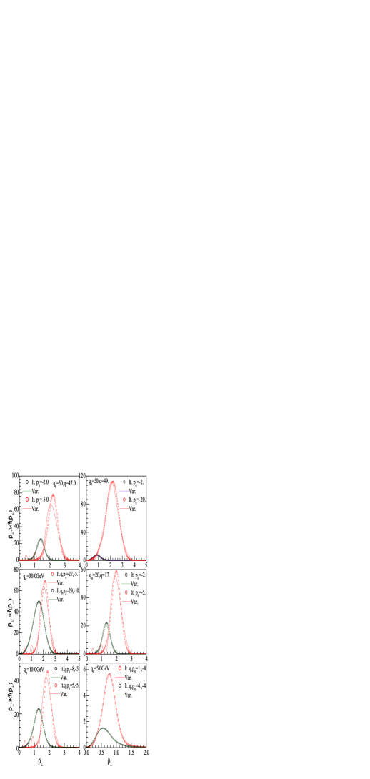
Figure 5: The ${\bf p_{\perp}}$ distributions ${\bf\tilde{p}_{\perp}}\cdot\Re{\bf\tilde{f}(\tilde{p}_{\perp})}$ for aws process. The symbols represent the results from iterations for some cases of $\{p_{0},q_{0},Q^{2}\}$ values studied. Different colored symbols represent different quark momenta. The results of variational method are shown by curves. The terms It. and Var. in figure labels refer to iterations and variational methods.

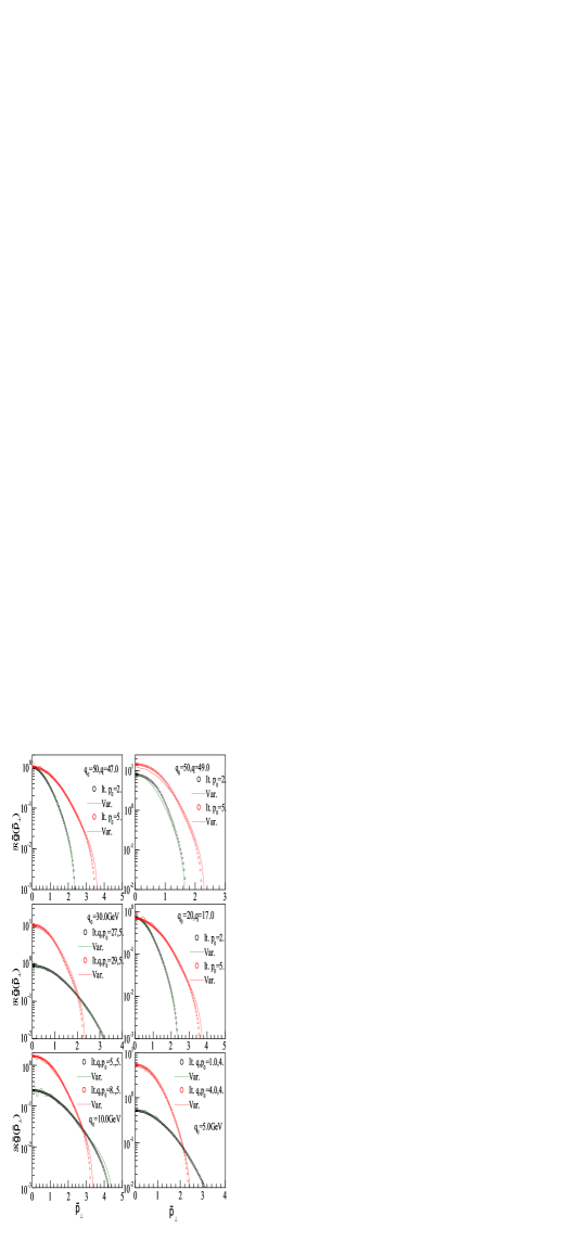
Figure 6: The ${\bf p_{\perp}}$ distributions $\Re{\tilde{g}(\tilde{\bf p}_{\perp})}$ (longitudinal part) of bremsstrahlung photon emission. The other details are as in Figure. 4.

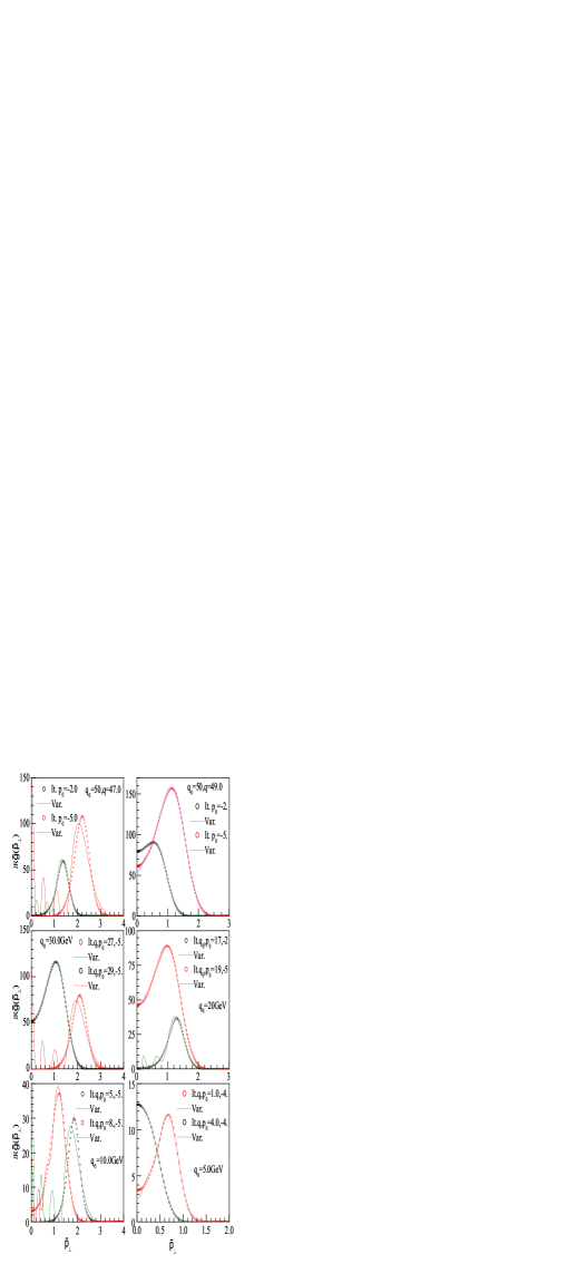
Figure 7: The ${\bf p_{\perp}}$ distributions $\Re{\tilde{g}(\tilde{\bf p}_{\perp})}$ (longitudinal part) of aws process The oter details are as in Figure. 5.

Figure 5 shows the ${\bf p_{\perp}}$ distributions ${\bf\tilde{p}_{\perp}}\cdot\Re{\bf\tilde{f}(\tilde{p}_{\perp})}$ of ${\bf aws}$ process for five values of $q_{0}=50,30,20,10,5$ GeV. For each $q_{0}$, similar to previous figure, distributions for two quark momenta values are shown . Figure 6 shows the ${\bf p_{\perp}}$ distributions ${\Re{\tilde{g}}({\bf\tilde{p}}_{\perp})}$ of bremsstrahlung process for five values of $q_{0}$. Figure 7 shows the ${\bf p_{\perp}}$ distributions for ${\Re{\tilde{g}}({\bf\tilde{p}}_{\perp})}$ of (longitudinal part of) ${\bf aws}$ process for five values of $q_{0}$.
The ${\bf p_{\perp}}$ distributions presented in Figures 4-7 proved the validity of variational method. For low $Q^{2}$ this method can be applied to study the LPM effects in virtual photon emission. However, the variational parameter needs to be optimized as it is not known for virtual photon case. For the case of real photons, we have shown an empirical estimate for the optimized variational parameter in terms of real photon dynamical variable $x_{1}$. For the case of virtual photon emission such a simple empirical formula in terms of $x_{1}$ is not valid and this should be a function also of $Q^{2}$. Therefore, in order to predict the optimized variational parameter for virtual photon emission case, we propose to examine the peak positions values of $\bf p_{\perp}$ distributions from iterations method. In Eqs.42-45 we define four dimensionless variables used in the following work. Especially, $x^{b}_{T}$ of Eq.45 is the relevant dynamical variable for virtual photon emission at high $Q^{2}$ and the variable $x_{1}$ is for real photons. (inverse of $x$ variable used in svsprc ). We searched for the peak position values of ${\bf p_{\perp}}$ distributions from the iterations method. These are functions of $p_{0},q_{0},Q^{2}$ and we searched for dynamical variables that could represent the peak positions for virtual photon case.

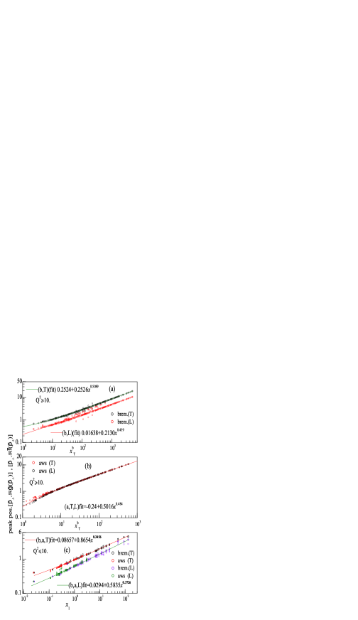
Figure 8: The peak positions of the ${\bf\tilde{p}_{\perp}}\cdot{\bf\Re\tilde{f}}({\bf\tilde{p}_{\perp}})$ and ${\tilde{p}_{\perp}}\cdot\Re\tilde{g}({\bf\tilde{p}_{\perp}})$ distributions corresponding to various processes and photon virtuality $Q^{2}$ and quark momenta. All data points shown are peak position results obtained from iterations method. The solid curves are the empirical power law fits shown on the figures. One should note that the x-scale is $x^{b}_{T}$ for figures (a,b) and scale is $x_{1}$ for figure (c) (for details see text). These empirical fits give a rough estimate of the optimized variational parameter for use in variational method. The labels b,a represent the processes. The lables T,L represent components.

$$x_{0} = \frac{|(p_{0}+q_{0})p_{0}|}{q_{0}T}$$ (42)

$$x_{1} = x_{0}\frac{M_{\infty}^{2}}{m_{D}^{2}}$$ (43)

$$x_{2} = x_{0}\frac{Q^{2}}{q_{0}T}$$ (44)

$$x^{b}_{T} = x_{1}+x_{2}$$ (45)

Figure 8(a) shows the peak positions of the (transverse) ${\bf\tilde{p}_{\perp}}\cdot{\bf\Re\tilde{f}}({\bf\tilde{p}_{\perp}})$ and (longitudinal) ${\tilde{p}_{\perp}}\Re\tilde{g}({\bf\tilde{p}_{\perp}})$ distributions for bremsstrahlung process at $Q^{2}\geq 10GeV^{2}$. The data is generated by solving the integral equations using iterations method for the set of values $\{p_{0},q_{0},Q^{2}\}$. For the longitudinal part, the peak positions do not exist for several values of $p_{0},q_{0},Q^{2}$ and the corresponding $\Re\tilde{g}({\bf\tilde{p}_{\perp}})$ distributions exhibit a Woods-Saxon form as can be seen in Figs.6,7. However, the integrand of $\int d^{2}{\bf\tilde{p}_{\perp}}\Re\tilde{g}({\bf\tilde{p}_{\perp}}),~{}{\it i.e.,}~{}{\tilde{p}_{\perp}}\Re\tilde{g}({\bf\tilde{p}_{\perp}})$, exhibits peaking behaviour. Therefore, we propose that the variational paramter may be fixed as the peak positions of these respective distributions. One should notice the $x$-scale is $x^{b}_{T}$ as defined in Eq.45 for both transverse and longitudinal distributions. The data is fitted by a function whose formula and the coefficients are mentioned in the figure (a) for both transverse and longitudinal parts. We have chosen a fitting function of type $y=a+bx^{p}$ because, as $x\rightarrow 0$, we want the peak positions to saturate as in real photon case (for real photons $A_{v}\geq 0.31$).
Figure 8(b) shows the similar results for ${\bf aws}$ process at $Q^{2}\geq 10GeV^{2}$. Here again the $x$ scale is $x^{b}_{T}$. Moreover, the distributions ${\bf\tilde{p}_{\perp}}\cdot{\bf\Re\tilde{f}}({\bf\tilde{p}_{\perp}})$, ${\tilde{p}_{\perp}}\Re\tilde{g}({\bf\tilde{p}_{\perp}})$ have approximately same peak position values for different $p_{0},q_{0},Q^{2}$. The fit functions and coefficients are shown in Figure 8(b).
Figure 8(c) shows the peak positions for bremsstrahlung and ${\bf aws}$ process for $Q^{2}\leq 10GeV^{2}$. In this figure, the transverse distributions (i.e., ${\bf\tilde{p}_{\perp}}\cdot{\bf\Re\tilde{f}}({\bf\tilde{p}_{\perp}}))$ for bremsstrahlung and ${\bf aws}$ have approximately same peak positions for different $p_{0},q_{0},Q^{2}$ values. Notice that the $x$ scale is the $x_{1}$ variable defined in Eq.43. Surprisingly, all these peak position values scale with $x_{1}$ variable rather than the usual $x^{b}_{T}$ for transverse components. This might be indicating that for small virtuality, the relevant scale is $x_{1}$, coinciding with real photon scale. Similarly, the longitudinal components ${\tilde{p}_{\perp}}\Re\tilde{g}({\bf\tilde{p}_{\perp}})$ have same peak positions for these two processes. The fit functions and coefficients are shown in figure. Using the formulae given in Figures.8(a,b,c) for the case of virtual photon emission, one may choose the variational parameter $A_{v}(p_{0},q_{0},Q^{2})$ to be around these peak position values.
It is interesting to compare the results for real and virtual photon peak positions. The peak positions of ${\bf\tilde{p}_{\perp}}\cdot{\bf\Re\tilde{f}}({\bf\tilde{p}_{\perp}})$ distributions for real photons are given by empirical fits in Fig.3(c). The peak positions of ${\bf\tilde{p}_{\perp}}\cdot{\bf\Re\tilde{f}}({\bf\tilde{p}_{\perp}})$,  ${\tilde{p}_{\perp}}\Re\tilde{g}({\bf\tilde{p}_{\perp}})$ distributions for virtual photons for $Q^{2}\leq 10GeV^{2}$ are given in Fig.8(c). In Figure 9, we compare these three results. As seen in figure, the peak positions for real photon and the transverse part of virtual photons are approximately the same. It should be noted that the numerical calculations have errors such as the iterations method has convergence errors, peak search has errors, errors in empirical fit of peak positions etc. Further, $\alpha_{s}$ value used is 0.2 for real photons and 0.3 for virtual photon studies. This close matching of peak positions of real and virtulal cases is rather surprising, as a strong $Q^{2}$ dependence is expected for virtual photons. Similar surprising results were already presented in gef regarding photon emission function.

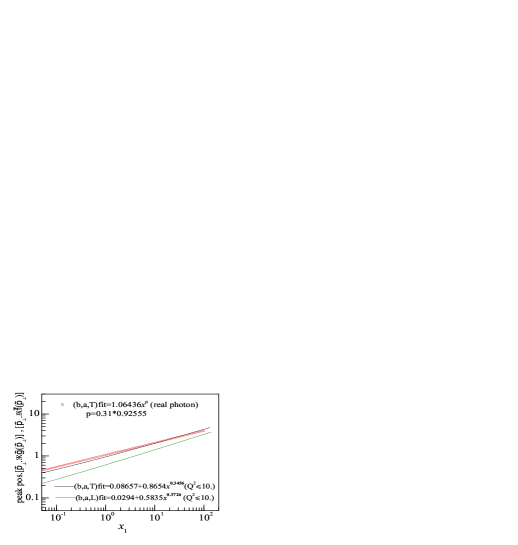
Figure 9: The peak positions of the ${\bf\tilde{p}_{\perp}}\cdot{\bf\Re\tilde{f}}({\bf\tilde{p}_{\perp}})$ for real photons represented by red circles, same as in Fig.3(c). The peak positions ${\bf\tilde{p}_{\perp}}\cdot{\bf\Re\tilde{f}}({\bf\tilde{p}_{\perp}})$,  ${\tilde{p}_{\perp}}\Re\tilde{g}({\bf\tilde{p}_{\perp}})$ distributions corresponding to various processes and photon virtuality $Q^{2}\leq 10GeV^{2}$ are shown by black curve and green curve respectively.

$$\Im{\Pi^{\mu}}_{R\mu} \sim \int_{-\infty}^{\infty}dp_{0}[n_{F}(r_{0})-n_{F}(p_{0})]\otimes$$ (46)

$$\int\frac{d^{2}{\bf\tilde{p}_{\perp}}}{(2\pi)^{2}}\left[\frac{p_{0}^{2}+r_{0}^{2}}{2(p_{0}r_{0})^{2}}\Re{\bf\tilde{p}_{\perp}.\tilde{f}(\tilde{p}_{\perp})}+\right.$$

$$\left.\frac{1}{\sqrt{\left|p_{0}r_{0}\right|}}\frac{Q^{2}}{q^{2}}\left(\frac{1}{m_{D}}\right)\Re\tilde{g}({\bf\tilde{p}_{\perp}})\right]$$

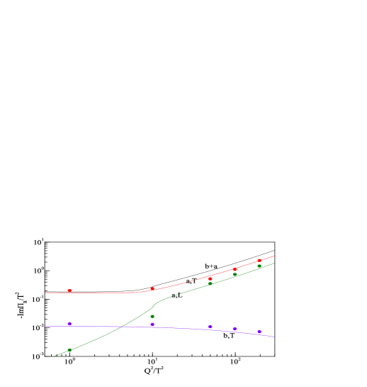
Figure 10: $\Im\Pi_{R}$ plotted as a function of $Q^{2}/T^{2}$ for a photon energy of 50GeV. The transverse components of bremsstrahlung, $\bf aws$, the insignificant contribution from longitudinal parts are shown. Symbols represent variational calculations. For reference the curves shown are taken from gef .

In the previous section, we compared the results from variational and iterations methods and gave empirical fits to optimized values of variational parameters. Using the variational method and the variational parameters given in Figures.8a,b,c, we repeated the variational calculations for all the values of $\{q_{0},q,p_{0}\}$. These calculations cover transverse and longitudinal parts of bremsstrahlung and $\bf aws$ processes for which we have reference distributions from iterations method. Now, we compared these two sets of $p_{\perp}$ distributions. It was noticed that the transverse bremsstrahlung distributions were exactly reproduced for all $\{q_{0},q,p_{0}\}$ values. The longitudinal contributions to bremsstrahlung were not not well reproduced, as the variational data showed oscillations around the iterations distributions. The transverse and longitudinal parts of $\bf aws$ were reasonably well reproduced for all $Q^{2}\leq 100GeV^{2}$. The $\bf aws$ distributions showed sensitivity to variational parameter. Therefore, it should be noted that the empirical optimized variational parameter is a good approximation, however, one needs to vary the variational parameter around these empirical values to converge the variational results.
The imaginary part of retarded photon polarization tensor (represented by $\Im\Pi_{R}$) is calculated using the $\bf p_{\perp}$ integrated values as given in Eq.46 (see Eq.16 of lpmdilep ). The required $\bf p_{\perp}$ integrated values were generated using variational method with empirical variational parameters. In this Eq.46, one should note the factor $1/m_{D}$ in the longitudinal part for reasons explained before. All terms in this equation contributing to $\Im\Pi_{R}$ are calculated. Figure 10 shows the $\Im\Pi_{R}$ plotted as a function of $Q^{2}/T^{2}$ for a photon energy of 50GeV. The results of variational method are represented by symbols in the figure. The transverse components of bremsstrahlung and $\bf aws$ represented in figure by b,T and a,T. The longitudinal contribution to $\bf aws$ is shown as a,L. The results from variational method (symbols) for various components have been normalized to approximately match with respective curves at $Q^{2}/T^{2}=1$. At this photon energy (50GeV), the contribution of bremsstrahlung is completely negligible. The bremsstrahlung is insignificant because the $q_{0}$ is very high. The transverse component of $\bf aws$ only contributes, with a small contribution from longitudinal component above $Q^{2}>20GeV^{2}$. The curves represent the imaginary polarization tensor by empirical method proposed in gef . It can be seen that the variational has predicted reasonably well the the results of gef for $Q^{2}/T^{2}$ in the range of  $1-250$. As shown in lpmdilep , the multiple re-scatterings in the medium only marginally increase the $\Im\Pi_{R}$ at low $Q^{2}$. However, the re-scattering corrections smooth out the discontinuity at the tree level threshold $Q^{2}=4M_{\infty}^{2}$ lpmdilep .

IV Conclusion

The photon emission processes from the quark gluon plasma have been studied as a function of photon mass, considering LPM suppression effects at a fixed temperature of the plasma. Self-consistent iterations method and the variational method have been used to solve the AMY and AGMZ integral equations. We obtained the ${\bf\Re\tilde{f}}({\bf\tilde{p}_{\perp}})$, ${\Re\tilde{g}}({\bf\tilde{p}_{\perp}})$ distributions as a function of photon mass, photon energy and quark momentum. The corresponding distributions from variational method have been compared with the results of iterations method for validating the variational approach. In order to fix variational parameter, the peak positions of the $\bf p_{\perp}$ distributions have been studied in detail for both real and virtual photons emission using iteration method. We identified relevant dynamical scales for the peak position values for real and virtual photon cases. The peak positions have been represented using appropriate dynamical scales and fitted with empirical formulae. In terms of these formulae, the optimized variational parameter can be approximately estimated. Using this empirical variational parameter, imaginary part of retarded photon polarization tensor has been calculated at photon energy of 50GeV.

- (1) Thomas Peitzman and Markus H. Thoma, hep-ph/0111114.
- (2) Charles Gale L. Haglin, and [hep-ph/0306098v3]; Charles Gale, hep-ph/0512109v2
- (3) R. Rapp, [hep-ph/0204003v1]
- (4) J.I. Kapusta, P. Lichard, D. Seibert, Phys. Rev. D 44, 2774 (1991).
- (5) R. Baier, H. Nakkagawa, A. Niegawa, K. Redlich, Z. Phys. C 53, 433 (1992).
- (6) E. Braaten, R.D. Pisarski, Nucl. Phys. B 337, 569 (1990).
- (7) P. Aurenche, F. Gelis, R. Kobes and E. Petitgirard, Phys . Rev. D54 5274 (1996) [hep-ph/9604398]; Z. Phys. ,315 (1997) [hep-ph/9609256].
- (8) P. Aurenche, F. Gelis, R. Kobes and H. Zaraket, Phys. Rev. D58 085003 (1998), [hep-ph/9804224] ; D61 116001 (2000) [hep-ph/9911367]
- (9) P. Aurenche, F. Gelis, and H. Zaraket, JHEP 0207, 063 (2002); D62 096012 (2000) [hep-ph/0003326]
- (10) Peter Arnold, Guy D. Moore and Laurence G. Yaffe, JHEP 11 (2001) 057, [hep-ph/0109064].
- (11) Peter Arnold, Guy D. Moore and Laurence G. Yaffe, JHEP 12 (2001) 009, [hep-ph/0111107]
- (12) L.D. Landau, I.Ya. Pomeranchuk, Dokl. Akad. Nauk. SSR 92, 535 (1953).
- (13) L.D. Landau, I.Ya. Pomeranchuk, Dokl. Akad. Nauk. SSR 92, 735 (1953).
- (14) A.B. Migdal, Phys. Rev. 103, 1811 (1956).
- (15) S. V. S. Sastry, Phys. Rev. C67, 041901(R) (2003), [hep-ph/0211075]
- (16) S. V. S. Sastry, hep-ph/0208103.
- (17) T. Altherr, P.V. Ruuskanen, Nucl. Phys. B 380, 377 (1992).
- (18) M.H. Thoma, C.T. Traxler, Phys. Rev. D 56, 198 (1997), [hep-ph/09701354]
- (19) P. Aurenche, F. Gelis, Guy D. Moore and H. Zaraket, JHEP 12 (2002) 006, [hep-ph/0211036].
- (20) P. Aurenche, F. Gelis, and H. Zaraket, JHEP 05, 043 (2002)
- (21) S.V. Suryanarayana, hep-ph/0606056.
- (22) S.V. Suryanarayana, DAE-BRNS Nucl. Phys. Symposium, 47B, 448 (2004).