Probing long-range leptonic forces with solar and reactor neutrinos

Abstract

In this work we study the phenomenological consequences of the existence of long-range forces coupled to lepton flavour numbers in solar neutrino oscillations. We study electronic forces mediated by scalar, vector or tensor neutral bosons and analyze their effect on the propagation of solar neutrinos as a function of the force strength and range. Under the assumption of one mass scale dominance, we perform a global analysis of solar and KamLAND neutrino data which depends on the two standard oscillation parameters, $\Delta m^{2}_{21}$ and $\tan^{2}\theta_{12}$, the force coupling constant, its range and, for the case of scalar-mediated interactions, on the neutrino mass scale as well. We find that, generically, the inclusion of the new interaction does not lead to a very statistically significant improvement on the description of the data in the most favored MSW LMA (or LMA-I) region. It does, however, substantially improve the fit in the high-$\Delta m^{2}$ LMA (or LMA-II) region which can be allowed for vector and scalar lepto-forces (in this last case if neutrinos are very hierarchical) at 2.5 $\sigma$. Conversely, the analysis allows us to place stringent constraints on the strength versus range of the leptonic interaction.

Keywords: neutrino properties, solar and atmospheric neutrinos

1 Introduction

Many extensions of the standard model of particle physics predict the existence of new forces; either generating deviations of the gravitational law at short distances or predicting low mass particles whose exchange will induce new forces at long distances, generally violating the equivalence principle [1, 2]. A number of experiments have been searching for such new forces but no evidence has yet been found. These null results, nevertheless, provide very significant constraints on particle physics models, gravitational physics and even on cosmological speculations [2, 3].

We know that there are two long-range forces in nature, namely the electromagnetic and the gravitational force, but there is no a priori reason why only these two should exist. Since the seminal work of Lee and Yang [4] it has become standard to consider long-range forces coupling to baryon and/or lepton number. These would definitely violate the universality of free fall and thus can be tested by Eötvös-type experiments, as pointed out in [4]. In particular, Okun [5] used this idea to establish a bound on the strength of an hypothetical vectorial leptonic force; see [6] for a recent review. He obtained the bound on the “fine structure” constant

$$k_{V}<10^{-49}\,.$$ (1)

The lepton flavour symmetries, as several solar, atmospheric, as well as KamLAND, K2K and MINOS neutrino experiments indicate, cannot be exact in nature. If an electronic force exists, we may expect it to be of arbitrary but finite range. Notice that when the range is less than the Earth-Sun distance, the bound (1) is no longer valid. Other experiments [2, 3] using the Earth instead of the Sun as the electronic source derive bounds, which, however, are much less strict than (1).

Recently, it has been shown that neutrino physics allow to place quite stringent bounds on these new interactions. The impact of vector-like long-range forces coupled to lepton flavour numbers on solar and atmospheric neutrino experiments has been investigated in [7] and [8], respectively. It has been estimated in [7] that the fine structure constant coupled to electronic number $L_{e}$ $k_{V}(e)<6.4\times 10^{-54}$ to be compatible with solar neutrino oscillations. According to [8] atmospheric neutrino data can constrain the strength of forces coupled to $L_{e}-L_{\mu}$, $k_{V}(e\mu)\leq 5.5\times 10^{-52}$, and to $L_{e}-L_{\tau}$, $k_{V}(e\tau)\leq 6.4\times 10^{-52}$ (at 90% CL) when the range of the force is the Earth-Sun distance. Also, new forces coupling individually to the muonic or tauonic number can be constrained, producing, however, weaker bounds. In particular, primordial nucleosynthesis considerations provide the bound $k_{V}(\mu,\tau)<1.8\times 10^{-11}$ [9].

In the present paper, we would like to continue the line of research started in [7]. We perform a global analysis of the solar and KamLAND neutrino data with the objective of constraining new electronic forces. Since long-range forces can be mediated by the exchange of massless or very light bosons of spin $J=0,1$ and 2, we study all these cases. In the next Section the formalism to take into account the effects of scalar (S), vector (V) and tensor (T) forces in neutrino oscillations is worked out. In Section 3 we perform the analysis and we devote the final Section to our conclusions.

2 Formalism: Effects in Solar Neutrino Oscillations

If there is a new force coupled to the leptonic flavour numbers, its presence will affect neutrino oscillations when neutrinos travel through regions where a flavour dependent density of leptons is present as it is the case for solar neutrinos.

As we will see more in detail, how the effect of the new interaction on the oscillation pattern depends on its Lorentz structure. Nevertheless, it can be easily proved that for scalar, vector or tensor interactions of large enough range the modification of the evolution equation can always be casted in terms of a unique function which solely depends on the background density of leptons – the source of the force – and the range of the interaction.

In particular, in the Sun, we can define a universal function $W$ determining the effect of a new force coupled uniquely to $L_{e}$ at a point $r$ from the center of the Sun:

$$W(r)=\int_{0}^{R_{\rm Sun}}d^{3}\rho\ n_{e}(\rho)\frac{e^{-\,|\vec{\rho}-\vec{r}|/\lambda}}{|\vec{\rho}-\vec{r}|}\,,$$ (2)

where $R_{\rm Sun}$ is the radius of the Sun and $n_{e}(r)$ is the electron number density in the medium. The range of the interaction is $\lambda=1/m$, where $m$ is the exchanged boson mass. We can easily do the angular integration in (2) and get

$$W(r)=\frac{2\pi\lambda}{r}\int_{0}^{R_{\rm Sun}}d\rho\ n_{e}(\rho)\ \rho\left[e^{-\,|\rho-r|/\lambda}\,-\,e^{-\,(\rho+r)/\lambda}\right]\,.$$ (3)

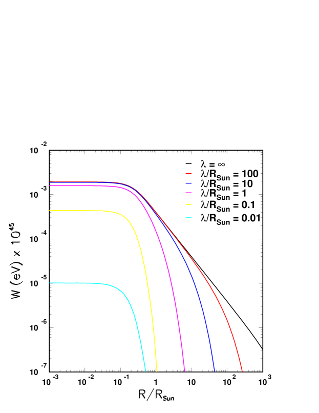
Figure 1: Leptonic potential function $W(r)$ due to the density of electrons in the Sun as a function of the distance from the solar center in units of $R_{\rm Sun}$ for various ranges $\lambda$.

In Figure 1 we show the function $W(r)$ in the Sun as a function of the distance in units of $R_{\rm Sun}$ for various ranges $\lambda$. As seen in the figure, inside the Sun and up to 0.1 $R_{\rm Sun}$, $W$ is constant independently of the range of the force considered. After that, it drops according to the force range and at the position of the Earth, at about 200 $R_{\rm Sun}$ from the center of the Sun, $W\raise 1.29167pt\hbox{$\;<$\kern-7.5pt\raise-4.73611pt\hbox{$\sim\;$}}2\times 10^{-39}$ eV.

In order to see the effect of the new $L_{e}$-coupled force in the evolution of solar neutrinos we have to take into account that at present the minimum joint description of atmospheric [10], K2K [11], MINOS [12], solar [13, 14, 15, 16, 17, 18] and reactor [19, 20] data requires that all the three known neutrinos take part in the oscillations. The mixing parameters are encoded in the $3\times 3$ lepton mixing matrix which can be conveniently parametrized in the standard form

$$U=\left(\begin{array}[]{ccc}1&0&0\\ 0&{c_{23}}&{s_{23}}\\ 0&-{s_{23}}&{c_{23}}\end{array}\right)\left(\begin{array}[]{ccc}{c_{13}}&0&{s_{13}}e^{i{\delta}}\\ 0&1&0\\ -{s_{13}}e^{-i{\delta}}&0&{c_{13}}\\ \end{array}\right)\left(\begin{array}[]{ccc}c_{21}&{s_{12}}&0\\ -{s_{12}}&{c_{12}}&0\\ 0&0&1\cr\end{array}\right)\,,$$ (4)

where $c_{ij}\equiv\cos\theta_{ij}$ and $s_{ij}\equiv\sin\theta_{ij}$.

According to the current data, the neutrino mass squared differences can be chosen so that

$$\Delta m^{2}_{\odot}=\Delta m^{2}_{21}\ll|\Delta m_{31}^{2}|\simeq|\Delta m_{32}^{2}|=\Delta m^{2}_{\rm atm}.$$ (5)

As a consequence of the fact that $\Delta m^{2}_{21}/|\Delta m^{2}_{31}|\approx 0.03$, for solar and KamLAND neutrinos, the oscillations with the atmospheric oscillation length are completely averaged and the interpretation of these data in the neutrino oscillation framework depends mostly on $\Delta m^{2}_{21}$, $\theta_{12}$ and $\theta_{13}$ (while atmospheric and long baseline neutrino oscillations are controlled by $\Delta m^{2}_{32}$, $\theta_{23}$ and $\theta_{13}$). Furthermore, the negative results from the CHOOZ reactor experiment [20] imply that the mixing angle connecting the solar and atmospheric oscillation channels, $\theta_{13}$, is severely constrained ($\sin^{2}\theta_{13}\leq 0.041$ at 3$\sigma$ [21]). Altogether, it is found that the 3-$\nu$ oscillations effectively factorize into 2-$\nu$ oscillations of the two different subsystems: solar (and reactor) and atmospheric (and long baseline).

Because the new interaction is flavour diagonal and its effect in the evolution of atmospheric neutrinos does not modify the hierarchy (5), the 2$\nu$ oscillation factorization still holds. Thus, in general, one can write the solar neutrino evolution equation in the presence of the new $L_{e}$-coupled force as

$$i\frac{d}{dr}\left(\begin{array}[]{c}\nu_{e}\\ \nu_{\mu}\end{array}\right)=\left[\frac{1}{2E_{\nu}}\mathbf{U}_{\theta_{12}}\;\mathbf{M^{2}}\;\mathbf{U}_{\theta_{12}}^{\dagger}+\left(\begin{array}[]{cc}V(r)&~{}0\\ \hphantom{-}0&~{}0\end{array}\right)\right]\left(\begin{array}[]{c}\nu_{e}\\ \nu_{\mu}\end{array}\right),$$ (6)

where

$$\mathbf{U}_{\theta_{12}}=\left(\begin{array}[]{cc}\cos\theta_{21}&{\sin\theta_{12}}\\ -{\sin\theta_{12}}&{\cos\theta_{12}}\end{array}\right),$$ (7)

and $\mathbf{M}$ and $V(r)$ will depend on the Lorentz structure of the new leptonic interaction as we describe next:

2.1 Scalar Interaction ($J=0$)

If the new force is mediated by a neutral spin $J=0$ particle, $\phi$, the interaction Lagrangian for the neutrinos will take the form:

$$L=-g_{0}\phi\bar{\psi}_{\nu}\psi_{\nu}\,.$$ (8)

We now use that the electron density can be taken to be the (static) source of the $L_{e}$-coupled interaction and that the neutrino will experience the force due to this source as long as within its range. In this approximation the effect of the new interaction can be included in the neutrino evolution equation as in (6) with:

$$\mathbf{M}=\left(\begin{array}[]{cc}m_{1}&0\\ 0&m_{2}\end{array}\right)-\mathbf{U}_{\theta_{12}}^{\dagger}\,\left(\begin{array}[]{cc}M_{\rm{S}}(r)&0\\ 0&0\end{array}\right)\,\mathbf{U}_{\theta_{12}}\qquad{\rm{and}}\qquad V(r)=V_{\rm{CC}}(r),$$ (9)

where $m_{1,2}$ are the neutrino masses in vacuum, $V_{\rm{CC}}(r)=\sqrt{2}\,G_{F}n_{e}(r)$ is the Mikheyev-Smirnov-Wolfenstein (MSW) potential and $M_{\rm{S}}(r)=k_{S}(e)W(r)$ is the new scalar-leptonic-force-induced mass term. Here $k_{S}(e)=\displaystyle\frac{g_{0}^{2}}{4\pi}$. Different from the vector and tensor cases, the $\nu_{e}$ survival probability will not only depend on $\Delta m_{21}^{2}=m_{2}^{2}-m_{1}^{2}$ but also on the value of the absolute neutrino mass scale $m_{1}$, which is still not experimentally known [22]. Notice also that the term $M_{S}(r)$ has the same sign for neutrinos and antineutrinos.

2.2 Vector Interaction ($J=1$)

If there is a new $L_{e}$-coupled vector force mediated by a neutral vector boson $A_{\alpha}$, the interaction Lagrangian for the neutrinos is:

$$L=-g_{1}A_{\alpha}\bar{\psi}_{\nu}\gamma^{\alpha}\psi_{\nu}\;.$$ (10)

In this case the neutrino evolution is described by (6) with

$$\mathbf{M}=\left(\begin{array}[]{cc}m_{1}&0\\ 0&m_{2}\end{array}\right)\qquad{\rm and}\qquad V(r)=V_{\rm CC}(r)+V_{\rm V}(r),$$ (11)

where $V_{\rm{V}}=k_{V}(e)W(r)$ is the lepto-vector potential with $k_{V}(e)=\displaystyle\frac{g_{1}^{2}}{4\pi}$. As a consequence of the vector structure of the force, the new leptonic potential adds to the MSW potential with the same energy dependence and sign. It will accordingly flip sign when describing antineutrino oscillations.

2.3 Tensor Interaction ($J=2$)

For a $L_{e}$-coupled force mediated by a tensor field of spin $J=2$, $\chi_{\alpha\beta}$, the interaction Lagrangian for the neutrinos is given by

$$L=-\frac{g_{2}}{2}\ \chi_{\alpha\beta}\left[\bar{\psi}_{\nu}\gamma^{\alpha}i\partial^{\beta}\psi_{\nu}-i\partial^{\alpha}\bar{\psi}_{\nu}\gamma^{\beta}\psi_{\nu}\right]\,,$$ (12)

where the coupling constant $g_{2}$ has dimensions $1/E$.

In this case the neutrino evolution is described by (6) with

$$\mathbf{M}=\left(\begin{array}[]{cc}m_{1}&0\\ 0&m_{2}\end{array}\right)\qquad{\rm and}\qquad V(r)=V_{\rm CC}(r)-V_{\rm T}(r).$$ (13)

$V_{\rm{T}}(r)=E_{\nu}k_{T}(e)W(r)$ is the tensorial potential and $E_{\nu}$ is the neutrino energy. Here $k_{T}(e)=m_{e}\displaystyle\frac{g_{2}^{2}}{4\pi}$ and $m_{e}$ is the mass of the electron.

Finally, let us remark that, as for the case of a scalar leptonic force, a tensor force is always symmetric when changing from neutrinos to antineutrinos. This is obvious from (12) since what we have coupled to the tensor field $\chi$ is in fact the energy momentum tensor of the leptons, which has to be symmetric under the exchange of particles and antiparticles.

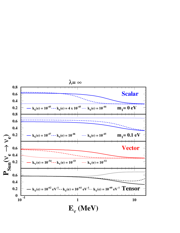
Figure 2: Survival probability of $\nu_{e}$ in the Sun as a function of the neutrino energy $E_{\nu}$ for an infinite range scalar (first two panels), vector (third panel) and tensor (lower panel) $L_{e}$-coupled force, for various values of the strength $k_{i}(e),\,i=S,V,T$. For all curves we have used $\tan^{2}\theta_{12}=0.44$ and $\Delta m^{2}_{21}=7.9\times 10^{-5}~{}{\rm{eV}}^{2}$.

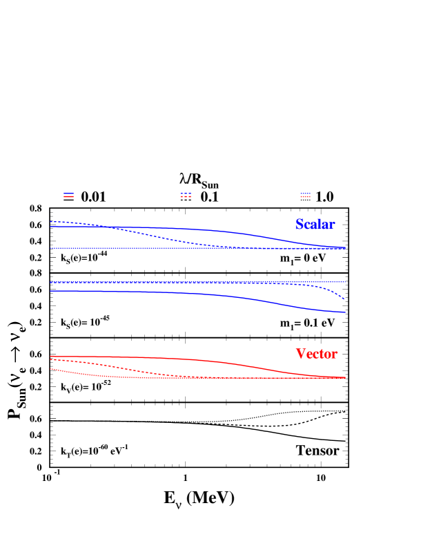
Figure 3: Same as Figure 2 but for $\lambda/R_{\rm Sun}=0.01,0.1$, and $1$.

Before performing the data analysis we can have some idea of the size of the effects of these long-range forces on neutrino oscillations by studying the value of the $\nu_{e}$ survival probability of solar neutrinos for different values of the coupling constant and range. The probability is obtained by solving (6) along the neutrino trajectory from its production point in the Sun to its detection point on the Earth. We have verified that for the range of parameters of interest the evolution in the Sun and from the Sun to the Earth is always adiabatic. It is interesting to remark that for the largest range forces the effective mixing angle at the surface of the Earth is still affected by the value of the leptonic potential produced by the Sun electron density.

We show in Figure 2 the survival probability of solar $\nu_{e}$ at the sunny face of the Earth as a function of the neutrino energy $E_{\nu}$ for an infinite range force. In the upper panels we show the scalar case for two extreme values of $m_{1}$, which correspond to strong mass hierarchy ($m_{1}=0$) and degenerate spectrum ($m_{1}=0.1$ eV), and some values of $k_{S}(e)$. From this figure we can foresee that for $m_{1}=0$, values of $k_{S}(e)\gtrsim 10^{-45}$–$10^{-44}$ will conflict with the existing solar neutrino data while for $m_{1}=0.1$ eV even smaller values of the coupling, $k_{S}(e)\gtrsim 10^{-46}$–$10^{-45}$, will be ruled out. In the third panel we show the vector case for some values of $k_{V}(e)$. One expects from this that our analysis will lead to bounds $k_{V}(e)\raise 1.29167pt\hbox{$\;<$\kern-7.5pt\raise-4.73611pt\hbox{$\sim\;$}}10^{-54}$–$10^{-53}$. Finally, in the lower panel the tensor case is displayed. In this case one expects that the data will constrain $k_{T}(e)\raise 1.29167pt\hbox{$\;<$\kern-7.5pt\raise-4.73611pt\hbox{$\sim\;$}}10^{-61}-10^{-60}$ eV^-1.

The dependence of the $\nu_{e}$ survival probability on the range $\lambda/R_{\rm Sun}$ can seen in Figure 3. From this plot we can see how the limit on $k$ will weaken as we allow for the force to have a finite range.

3 Constraints from Solar and Reactor Neutrino Data

We present in this section the results of the global analysis of solar and KamLAND data for the long-range forces discussed in the previous section.

Details of our solar neutrino analysis have been described in previous papers [23, 24]. We use the solar fluxes from Bahcall et al [25]. The solar neutrino data includes a total of 119 data points: the Gallium [14, 15] (2 data points) and Chlorine [13] (1 data point) radiochemical rates, the Super-Kamiokande [16] zenith spectrum (44 bins), and SNO data reported for phase 1 and phase 2. The SNO data used consists of the total day-night spectrum measured in the pure D₂O (SNO-I) phase (34 data points) [17], plus the full data set corresponding to the Salt Phase (SNO-II) [18]. This last one includes the NC and ES event rates during the day and during the night (4 data points), and the CC day-night spectral data (34 data points). It is done by a $\chi^{2}$ analysis using the experimental systematic and statistical uncertainties and their correlations presented in [18], together with the theoretical uncertainties. In combining with the SNO-I data, only the theoretical uncertainties are assumed to be correlated between the two phases. The experimental systematics errors are considered to be uncorrelated between both phases.

In the analysis of KamLAND, we neglect the effect of the long range forces due to the small Earth-crust electron density in the evolution of the reactor antineutrinos and we directly adapt the $\chi^{2}$ map as given by the KamLAND collaboration for their unbinned rate+shape analysis [26] which uses 258 observed neutrino candidate events and gives, for the standard oscillation analysis, a $\chi^{2}_{\rm min}$=701.35. The corresponding Baker-Cousins $\chi^{2}$ for the 13 energy bin analysis is $\chi^{2}_{\rm min}=13.1/11$ dof.

3.1 Scalar Interaction

In the scalar case the analysis of solar and KamLAND data depends on 6 parameters: the two oscillation parameters, $\Delta m^{2}_{21}$ and $\tan^{2}\theta_{12}$, the absolute neutrino mass scale $m_{1}$, the coupling $k_{S}(e)$ and the range of the force $\lambda/R_{\rm Sun}$. We have done our analysis fixing $m_{1}$ at two extreme values, $m_{1}=0$ and 0.1 eV.

For $m_{1}=0$ eV ($0.1$ eV) we find that the best fit point is

$$\tan^{2}\theta_{12}=0.49\;(0.44) \qquad\Delta m^{2}_{21}=7.9\times 10^{-5}~{}{\rm eV}^{2}\;(7.9\times 10^{-5}~{}{\rm eV}^{2})$$

$$\lambda/R_{\rm Sun}=1.26\;({\rm indet}) \qquad k_{S}(e)=5\times 10^{-45}\;(0)\;$$

$$\Delta\chi^{2}_{\rm{min}}=-1.4\;(0)\,,$$ (14)

where the range of the interaction is indeterminate (indet) when $k_{S}(e)=0$ and $\Delta\chi^{2}_{\rm{min}}$ is the shift in $\chi^{2}$ compared to the best fit point in the absence of a new $L_{e}$-couple force for which

$$\tan^{2}\theta_{12}=0.44~{} \qquad{\rm and}\qquad ~{}\Delta m^{2}_{21}=7.9\times 10^{-5}~{}{\rm eV}^{2}\,.$$ (15)

Thus we find that for highly hierarchical neutrinos the presence of the long range force can lead to a small improvement of the quality of the fit but this improvement is not statistically very significant leading only to a decrease of less than two units in $\chi^{2}$ even at the cost of introducing two new parameters. For degenerate neutrinos, on the contrary, the presence of the long-range force does not improve the agreement with the data.

This is further illustrated in Figure 4 where we show the result of the global analysis of solar data plus KamLAND data in the form of the allowed two-dimensional regions at 3$\sigma$ CL in the $(\Delta m^{2}_{21},\tan^{2}\theta_{12})$ plane after marginalization over $k_{S}(e)$ and $\lambda$. The standard MSW allowed region is also showed for reference. As seen in the figure for any value of $m_{1}$ the presence of the long-range forces has a mild (or null) impact on the allowed range of $\Delta m^{2}_{21}$ and $\tan^{2}\theta_{12}$ in the low-$\Delta m^{2}$ island, known as large mixing angle region I (LMA-I).

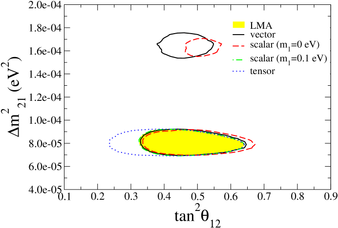
Figure 4: Allowed regions from the global analysis of solar plus KamLAND data in the $(\Delta m^{2}_{21},\tan^{2}\theta_{12})$ parameter space at 3$\sigma$ CL (2dof) for the different type of long-range forces as labeled in the figure. The standard MSW allowed region (shaded area) is also shown for reference.

Most interestingly, we also find that in the presence of the long-range scalar force the description of the solar data in the high-$\Delta m^{2}$ (LMA-II) region can be significantly improved if neutrinos are very hierarchical. As a consequence, in this case, there is a new allowed solution at the 98.9% CL. The best fit point in this region is obtained for

$$\tan^{2}\theta_{12}=0.5\qquad \qquad\Delta m^{2}_{21}=1.6\times 10^{-4}~{}{\rm eV}^{2}$$

$$\lambda/R_{\rm Sun}=4.0\;\qquad \qquad k_{S}(e)=6.9\times 10^{-45}\;\;$$

$$\Delta\chi^{2}_{\rm{min}}=7.2\;$$ (16)

While this region is excluded at more than 4$\sigma$ for the standard MSW oscillations it is allowed at 2.5$\sigma$ in the presence of a new scalar force for a narrow band of the lepto-force parameters. For example, for $\lambda=\infty$ the LMA-II region is allowed as long as $4.5\leq(k_{S}(e)/10^{-45})\leq 8.0$ .

The improvement of the fit in the LMA-II region can be understood as follows. For the range of scalar $L_{e}$-coupled lepto-forces that we are considering the neutrino evolution in the Sun is always adiabatic. Therefore the corresponding survival probability is determined by the effective mixing angle at the neutrino production point, $r_{0}$, which takes the form

$$S2_{12,m}=\frac{S2_{12}\Delta m^{2}_{21,S}}{\sqrt{[\Delta m^{2}_{21,S}C2_{12}-2E_{\nu}V_{CC}(r_{0})-M_{S}^{2}(r_{0})+M_{S}(r_{0})(m_{1}+m_{2})]^{2}+S2_{12}\Delta m^{2}_{21,S}}}$$ (17)

where we have defined $\Delta m^{2}_{21,S}=\Delta m_{21}^{2}-M_{S}(r_{0})\Delta m_{21}$ with $\Delta m_{21}=m_{2}-m_{1}$ and $S2_{12}=\sin 2\theta_{12}$, and $C2_{12}=\cos 2\theta_{12}$. As long as the term $M_{S}(r_{0})(m_{1}+m_{2})$ in the denominator is subdominant, the net effect of $M_{S}(r_{0})$ is to increase the effective matter potential and correspondingly, one can achieve a good fit to the solar data with higher values of $\Delta m^{2}_{21}$. In this case, the CL at which the LMA-II region is allowed is determined by KamLAND data [19] because the fit to the solar data cannot discriminate between the LMA-I and LMA-II regions once scalar $L_{e}$-coupled force effects are included. Clearly this implies that this solution will be further tested in the future by a more precise determination of the antineutrino spectrum at KamLAND.

As $m_{1}$ increases the term $M_{S}(r_{0})(m_{1}+m_{2})$ becomes more important and correspondingly the quality of the fit within the LMA-II region worsens. We find that for $m_{1}\gtrsim 0.02$ eV there is no LMA-II solution at 3$\sigma$.

We show in Figure 5 the survival probability for this best fit point in the high-$\Delta m^{2}$ (LMA-II) region in the presence of the scalar lepto-force together with the extracted average survival probabilities for the low energy ($pp$) , intermediate energy (⁷Be, $pep$ and CNO) and high energy solar neutrinos (⁸B and $hep$) from [28]. For comparison we also show the survival probability for conventional MSW oscillations for the same values of $\Delta m^{2}_{21}$ and $\theta_{12}$. From the figure it is clear that the inclusion of the lepto-force, leads to an improvement on the description of the solar data for all the energies being this more significant for intermediate- and high-energy neutrinos.

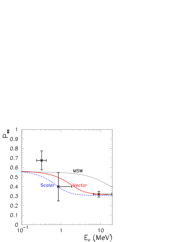
Figure 5: $\nu_{e}$ survival probability in the Sun versus neutrino energy for the best fit point in the high-$\Delta m^{2}$ region in the presence of scalar lepto-force with parameters given in (16) (full line) and for the vector lepto-force with parameters in (21). The dotted line is the survival probability for conventional MSW oscillations ($k_{i}=0$) for the same values of $\Delta m^{2}_{21}$ and $\theta_{12}$. The data points are the extracted average survival probabilities for the low energy ($pp$), intermediate energy (⁷Be, $pep$ and CNO) and high energy solar neutrinos (⁸B and $hep$) from [28].

Conversely, the global analysis of solar and KamLAND data results into constraints on the possible size of the new contribution to the neutrino mass. This is illustrated in Figure 6 where we show the result of the global analysis in the form of the allowed two-dimensional regions in the $(k_{S}(e),\lambda/R_{\rm Sun})$ parameter space after marginalization over $\Delta m^{2}_{21},\tan^{2}\theta_{12}$ for the two reference values of $m_{1}$.

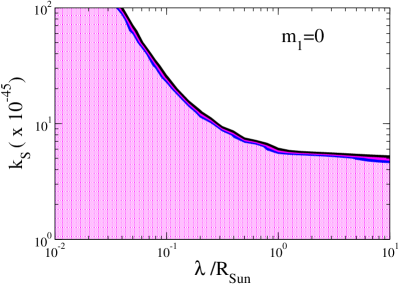
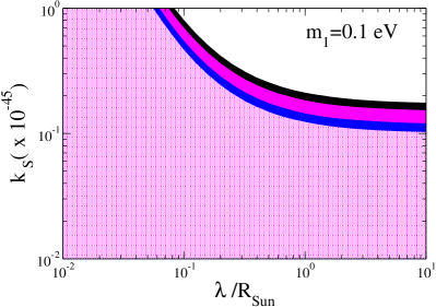
Figure 6: Allowed regions from the global analysis of solar plus KamLAND data in the $k_{S}(e)$ versus $\lambda/R_{\rm Sun}$ plane at 90%, 95%, 99% and 3$\sigma$ CL (2dof) for a $L_{e}$-coupled scalar force, with $m_{1}=0$ eV (left) and $m_{1}=0.1$ eV (right).

As seen in the figure, already at 90% CL (or lower) the regions are connected to the standard $k_{S}(e)=0,\;\lambda=\infty$ case. In other words, the analysis shows no evidence of any long-range $L_{e}$-coupled scalar force contributing to the solar neutrino evolution. However, as expected, there is a strong correlation between the implied bound on the strength and the range of the interaction. As discussed in the previous section the tightest bound on the strength of the new interaction corresponds to $\lambda=\infty$ (which effectively applies for $\lambda\gtrsim 10\,R_{\rm Sun}$)

$$k_{S}(e)\leq 5.0\times 10^{-45}\quad\quad(g_{0}\leq 2.5\times 10^{-22})\;\;\;\;\;\;\;{\rm for\;m_{1}=0\;\rm eV}\,,$$ (18)

$$k_{S}(e)\leq 1.5\times 10^{-46}\quad\quad(g_{0}\leq 4.3\times 10^{-23})\;\;\;\;\;\;\;{\rm for\;m_{1}=0.1\;\rm eV}\,,$$ (19)

at 3$\sigma$ (1dof).

3.2 Vector Interaction

If the new leptonic interaction is mediated by a vector boson the analysis of solar and KamLAND data depends on 4 parameters: the two oscillation parameters, $\Delta m^{2}_{21}$ and $\tan^{2}\theta_{12}$, the coupling $k_{V}(e)$ and the range of the force $\lambda/R_{\rm Sun}$.

In this case the best fit point corresponds to

$$\tan^{2}\theta_{12}=0.46\;\quad \quad\quad\Delta m^{2}_{21}=7.9\times 10^{-5}~{}{\rm eV}^{2}$$

$$\lambda/R_{\rm Sun}=2.5\times 10^{-3}\;\quad \quad\quad k_{V}(e)=7.9\times 10^{-51}\;\;$$

$$\Delta\chi^{2}_{\rm{min}}=-0.8\;,$$ (20)

which as for the scalar case represent a very small variation with respect to the standard LMA solution as seen in Figure 4.

From Figure 4 we also find that the presence of the vector lepto-force can improve the quality of the fit in the LMA-II region. This is possible because the lepto-force also adds up to the MSW potential and consequently the vacuum-matter transition condition $\Delta m^{2}_{21}\cos 2\theta=2E_{\nu}V(r_{0})$, which has to occur around $E_{\nu}\sim 1$ MeV to fit the data, can be achieved for a larger value of $\Delta m^{2}_{21}$.

So also in the vector case, there is a new allowed solution at 2.5 $\sigma$ CL. The best fit point in this region is obtained for

$$\tan^{2}\theta_{12}=0.46\quad \quad\quad\Delta m^{2}_{21}=1.6\times 10^{-4}~{}{\rm eV}^{2}$$

$$\lambda/R_{\rm Sun}=4.0\;\quad \quad\quad k_{V}(e)=6.9\times 10^{-45}\;\;$$

$$\Delta\chi^{2}_{\rm{min}}=7.9\;$$ (21)

The corresponding survival probability for this point is shown in Figure 5. The LMA-II region is allowed for a narrow band of $(k_{V}(e),\lambda/R_{\rm Sun})$ values. For example for $\lambda=\infty$ the LMA-II region is allowed as long as $2.0\leq(k_{V}(e)/10^{-54})\leq 30$.

As for the scalar lepto-force with hierarchical neutrinos, the CL at which the LMA-II region is allowed is determined by KamLAND data [19] and consequently this solution will be further tested by this experiment.

Concerning the allowed ranges of the lepto-force parameters, we show in Figure 7 the result of the global analysis in the form of the allowed two-dimensional regions in the $(k_{V}(e),\lambda/R_{\rm Sun})$ parameter space after marginalization over $\Delta m^{2}_{21},\tan^{2}\theta_{12}$. In particular we find that for $\lambda=\infty$

$$k_{V}(e)\leq 2.5\times 10^{-53}\;\;(g_{1}\leq 1.8\times 10^{-26})\,,$$ (22)

at 3$\sigma$ (1dof).

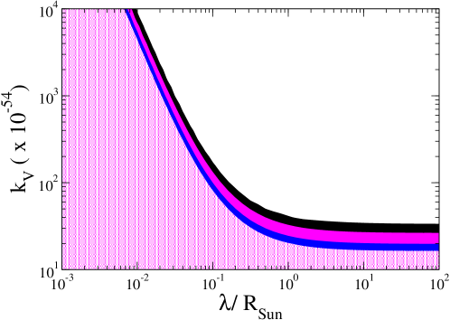
Figure 7: Allowed regions from the global analysis of solar plus KamLAND data in the $k_{V}(e)$ versus $\lambda/R_{\rm Sun}$ plane at 90%, 95%, 99% and 3$\sigma$ CL (2dof) for a $L_{e}$-coupled vector force.

3.3 $J=2$ Interaction

In the tensor case the analysis of solar and KamLAND data depends on 4 parameters: the two oscillation parameters, $\Delta m^{2}_{21}$ and $\tan^{2}\theta_{12}$, the coupling $k_{T}(e)$ and the range of the force $\lambda/R_{\rm Sun}$.

We find the best fit point at

$$\tan^{2}\theta_{12}=0.44\quad \quad\quad\Delta m^{2}_{21}=7.9\times 10^{-5}~{}{\rm eV}^{2}$$

$$\lambda/R_{\rm Sun}=({\rm indet})\quad \quad\quad k_{T}(e)=0\;$$

$$\Delta\chi^{2}_{\rm{min}}=0\;.$$ (23)

Thus for the case of the $J=2$ interaction there is no improvement on the quality of the fit compared to the standard MSW scenario.

From Figure 4 we see that the only effect of the inclusion of this interaction is the enlargement of the LMA-I region for smaller values of the mixing angle. The inclusion of the $J=2$ lepto-force decreases the effective matter potential (see (13)) at higher energies. As a consequence, as seen in Figures 2 and 3 the corresponding survival probability grows for the high end of the solar neutrino spectrum as compared to the standard MSW case. This behaviour can be compensated by a decrease of the vacuum mixing angle and leads to the enlargement of the allowed LMA-I region. However, because the effect of the $J=2$ lepto-force is to decrease the matter potential, no LMA-II solution is found in this case.

Finally, in Figure 8, we show the result of the global analysis in the form of the allowed two-dimensional regions in the $(k_{T}(e),\lambda/R_{\rm Sun})$ parameter space after marginalization over $\Delta m^{2}_{21}$ and $\tan^{2}\theta_{12}$. For $\lambda=\infty$ we obtain the bound

$$k_{T}(e)\leq 1.7\times 10^{-60}\;{\rm eV}^{-1}\;\;(g_{2}\leq 6.5\times 10^{-33}\;{\rm eV}^{-1})\,,$$ (24)

at 3$\sigma$ (1dof).

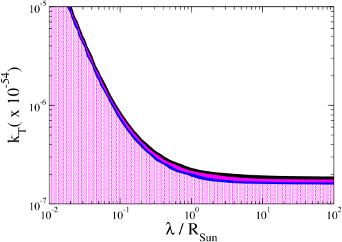
Figure 8: Allowed regions from the global analysis of solar plus KamLAND data in the $k_{T}(e)$ versus $\lambda/R_{\rm Sun}$ plane at 90%, 95%, 99% and 3$\sigma$ CL (2dof) for a $L_{e}$-coupled tensor force.

4 Conclusion and discussion

In this paper be have investigated the effects of long-range $L_{e}$-coupled forces in the oscillation of neutrinos in the Sun. Their impact on neutrinos depend on the spin of the exchanged particle leading to the new force. We have treated, in turn, the consequences of scalar, vector and tensor forces.

In our study we have used data from solar neutrino experiments and KamLAND. In the global fit, apart from the mass difference $\Delta m^{2}_{21}$ and the mixing angle $\theta_{12}$, which are the usual standard parameters, we have the new physics parameters $k_{i}$, the strength of the interaction with $i$=S,V,T, and the range $\lambda$ of the interaction. For the scalar case, we also need to assume the absolute mass scale for neutrinos.

The result of the global fit is that there is not a significant improvement in the description of the data in the preferred (in the standard case) MSW LMA region (LMA-I). However, the addition of new physics permits to “recover” the high-$\Delta m^{2}$ region (LMA-II) which is now allowed in the case of scalar and vector forces. Why this is so only for these forces and not for the tensorial one can be understood quite simply, as we have explained in the paper.

We have deduced limits on the strength of the forces for different values of the range $\lambda$ (see Figures 6, 7 and 8). For an infinite range ($\lambda=\infty$) $L_{e}$-coupled force, we get the following limits in terms of the “fine structure constants” $k_{i}$

$$k_{S}(e) \leq 5.0\times 10^{-45}\quad\quad(m_{1}=0\;{\rm eV})\,,$$ (25)

$$k_{S}(e) \leq 1.5\times 10^{-46}\quad\quad(m_{1}=0.1\;{\rm eV})\,,$$ (26)

$$k_{V}(e) \leq 2.5\times 10^{-53}\,,$$ (27)

$$k_{T}(e) \leq 1.7\times 10^{-60}\;{\rm eV}^{-1}\,,$$ (28)

at 3$\sigma$ (1dof).

These bounds are practically the same for any $\lambda\gtrsim 10\,R_{\rm Sun}$. For $\lambda\lesssim 10\,R_{\rm Sun}$, the bound slowly worsens, and for $\lambda\sim 0.1\,R_{\rm Sun}$ we have that the bound on $k_{i}$ is a factor less than 10 weaker than (25)-(28). In [7] the vectorial case was evaluated, not with the statistical rigor we have proceeded in the present paper. A bound on $k_{V}(e)$ one order of magnitude more stringent was found. Apart from extending the results to include scalar and tensor forces, our bound (27) supersedes the one in [7].

In deriving (25) to (28) we have assumed that the new force only couples to $L_{e}$ but the analysis can be easily extended to forces coupled to any linear combination of the lepton flavour numbers $L_{e}+\alpha L_{\mu}+\beta L_{\tau}$. For vector and tensor forces it can be easily proved that as long as the 2$\nu$-oscillation factorization holds, the bounds will be the ones given in (27) and (28) but they will constrain the combination $k_{V,T}=k_{V,T}(e)(1-\alpha\cos 2\theta_{23}-\beta\sin 2\theta_{23})$. In particular this means that for the anomaly-free combinations $L_{e}-L_{\mu}$, and $L_{e}-L_{\tau}$ the bounds on the corresponding $k_{V,T}(e\mu)$ and $k_{V,T}(e\tau)$ become tighter by a factor $1+\cos 2\theta_{23}\simeq 2$ and $1+\sin 2\theta_{23}\simeq 2$ respectively. For the case of the scalar interactions coupled to a general linear combination of lepton flavour numbers, the combination of couplings bounded depends on $m_{1}$ and it does not have such a simple expression as for the tensor and vector cases. But generically, provided that there is not a fine-tuned cancellation between the masses and the new interaction terms, the bound will be of the same order of magnitude as given in (25) and (26).

A final issue we should care about is the possibility of screening of leptonic charges by electronic neutrinos and antineutrinos from the cosmological relict background. As is explicitly demonstrated in [7], screening plays no role at the relevant scales on the order of the solar radius.

References

References

- [1] Damour T 1996 Class. Quantum Grav.13 A33 (Preprint gr-qc/9606080)
- [2] Fischbach E, Gillies G T, Krause D E, Schwan J G and Talmadge C 1992 Metrologia 29 213
- [3] Adelberger E G, Heckel B R and Nelson A E 2003 Ann. Rev. Nucl. Part. Sci. 53 77 (Preprint hep-ph/0307284) Fischbach E and Talmadge C 1998 The Search for Non-Newtonian Gravity (New York: Springer-Verlag)
- [4] Lee T D and Yang C N 1955 Phys. Rev.98 1501
- [5] Okun L 1969 Sov. J. Nucl. Phys. 10 206 Okun L 1996 Phys. Lett.B 382 389
- [6] Dolgov A D 1999 Phys. Rep. 320 1
- [7] Grifols J A and Masso E 2004 Phys. Lett.B 579 123 (Preprint hep-ph/0311141)
- [8] Joshipura A S and Mohanty S 2004 Phys. Lett.B 584 103
- [9] Grifols J A and Masso E 1997 Phys. Lett.B 396 201 (Preprint astro-ph/9610205)
- [10] Ashie Y et al(Super-Kamiokande Collaboration) 2005 Phys. Rev.D 71 112005
- [11] Aliu E et al(K2K Collaboration) 2005 Phys. Rev. Lett.94 081802
- [12] Tagg N (MINOS Collaboration) 2006 Proc. 4th Flavor Physics and CP Violation Conference (Vancouver) eConf C060409 (2006) 019 (Preprint hep-ex/0605058)
- [13] Cleveland B T et al1998 Astrophys. J. 496 505
- [14] Cattadori C 2004 Results from radiochemical solar neutrino experiments, talk given at XXIst International Conference on Neutrino Physics and Astrophysics (NU2004) (Paris)
- [15] Hampel W et al(GALLEX Collaboration) 1999 Phys. Lett.B 447 127
- [16] Fukuda S et al(Super-Kamiokande Collaboration) 2001 Phys. Rev. Lett.86 5651
- [17] Ahmad Q R et al(SNO Collaboration) 2001 Phys. Rev. Lett.87 071301 Ahmad Q R et al(SNO Collaboration) 2002 Phys. Rev. Lett.89 011302 Ahmed S N et al(SNO Collaboration) 2004 Phys. Rev. Lett.92 181301
- [18] Aharmim B et al(SNO Collaboration) 2005 Phys. Rev.C 72 055502 (Preprint nucl-ex/0502021)
- [19] Araki T et al(KamLAND Collaboration) 2005 Phys. Rev. Lett.94 081801 Eguchi K et al(KamLAND Collaboration) 2003 Phys. Rev. Lett.90 021802
- [20] Apolloni et al(CHOOZ Collaboration) 1998 Phys. Lett.B 420 397 Apolloni et al(CHOOZ Collaboration) 2003 Eur. Phys. J. C 27 331
- [21] Gonzalez-Garcia M C 2004 Preprint hep-ph/0410030
- [22] Bilenky S M, Giunti C, Grifols J A and Masso E 2033 Phys. Rept. 379 69 (Preprint hep-ph/0211462)
- [23] Bahcall J N, Gonzalez-Garcia M C and Peña-Garay C 2004 J. High Energy Phys. JHEP0408(2004)016 (Preprint hep-ph/0406294)
- [24] de Holanda P C and Smirnov A Yu 2004 Astropart. Phys. 21 287
- [25] Bahcall J N, Serenelli A M and Basu S 2005 Astrophys. J. 621 L85 Bahcall J N and Serenelli A M 2005 Astrophys. J. 626 530
-
[26]
KamLAND data and results are available at
http://www.awa.tohoku.ac.jp/KamLAND/datarelease/2ndresult.html
- [27] Gonzalez-Garcia M C, de Holanda P C and Zukanovich Funchal R 2006 Phys. Rev.D 73 033008 (Preprint hep-ph/0511093)
- [28] Barger V, Huber P and Marfatia D 2005 Phys. Rev. Lett.95 211802