Triumvirate of Running Couplings
in Small-$x$ Evolution

Abstract

We study the inclusion of running coupling corrections into the non-linear small-$x$ JIMWLK and BK evolution equations by resumming all powers of $\alpha_{s}N_{f}$ in the evolution kernels. We demonstrate that the running coupling corrections are included in the JIMWLK/BK evolution kernel by replacing the fixed coupling constant $\alpha_{s}$ in it with $\frac{\alpha_{s}(1/r_{1}^{2})\,\alpha_{s}(1/r_{2}^{2})}{\alpha_{s}(1/R^{2})}$, where $r_{1}$ and $r_{2}$ are transverse distances between the emitted gluon and the harder gluon (or quark) off of which it was emitted to the left and to the right of the interaction with the target. In the formalism of Mueller’s dipole model $r_{1}$ and $r_{2}$ are the transverse sizes of “daughter” dipoles produced in one step of the dipole evolution. The scale $R$ is a function of two-dimensional vectors ${\bf r}_{1}$ and ${\bf r}_{2}$, the exact form of which is scheme-dependent. We propose using a particular scheme which gives us $R$ as an explicit function of $r_{1}$ and $r_{2}$.

1 Introduction

In the recent years there has been a lot of progress in small-$x$ physics due to developments in the area of parton saturation and Color Glass Condensate (CGC) [1, 2, 3, 4, 5, 6, 7, 8, 9, 10, 11, 12, 13, 14, 15, 16, 17, 18, 19, 20, 21]. Among other things the CGC led to a new way of calculating the hadronic and nuclear structure functions and total cross sections in deep inelastic scattering (DIS) at small values of Bjorken $x$ variable. According to the CGC approach to high energy processes, one first has to calculate an observable in question in the quasi-classical limit of the McLerran-Venugopalan model [3, 4, 5] which resums all multiple rescatterings in the target hadron or nucleus. After that one has to include the quantum evolution corrections resumming all powers of $\alpha_{s}\,\ln 1/x_{Bj}$ along with all the multiple rescatterings. Such corrections are included in the general case of a large target by the Jalilian-Marian–Iancu–McLerran–Weigert–Leonidov–Kovner (JIMWLK) functional integro-differential equation [9, 10, 11, 12, 13, 14, 15, 16], or, if the large-$N_{c}$ limit is imposed, by the Balitsky-Kovchegov (BK) integro-differential evolution equation [19, 20, 21, 17, 18] based on Mueller’s dipole model [22, 23, 24, 25]. The JIMWLK and BK evolution equations unitarize the Balitsky-Fadin-Kuraev-Lipatov (BFKL) linear evolution equation [26, 27]. For detailed reviews of the physics of the Color Glass Condensate we refer the reader to [28, 29, 30].

Both the JIMWLK and BK evolution equations resum leading logarithmic $\alpha_{s}\,\ln 1/x_{Bj}$ corrections with $\alpha_{s}$ the coupling constant. At this leading order the running coupling corrections to the JIMWLK and BK evolution kernels are negligible next-to-leading order (NLO) corrections. A running coupling correction would bring in powers of, for instance, $\alpha_{s}^{2}\,\ln 1/x_{Bj}$, which are not leading logarithms anymore. Hence both JIMWLK and BK evolution equations do not include any running coupling corrections in their kernels. The drawback of this lack of running coupling corrections is that the scale of the coupling constant to be used in solving these evolution equations is not known. Indeed, as was argued originally by McLerran and Venugopalan [3, 4, 5] and confirmed by the numerical solutions of JIMWLK and BK equations [31, 32, 33, 34], the high parton density in the small-$x$ hadronic and nuclear wave functions gives rise to a hard momentum scale — the saturation scale $Q_{s}$. For small enough $x$ and for large enough nuclei this scale becomes much larger than the QCD confinement scale, $Q_{s}\gg\Lambda_{\text{QCD}}$. The existence of a large intrinsic momentum scale leads to the expectation that this scale would enter in the argument of the running coupling constant making it small and allowing for a perturbative description of the relevant physical processes. However, until now this expectation has never been confirmed by explicit calculations.

In the past there have been several good guesses of the scale of the running coupling in the JIMWLK and BK kernels in the literature [35, 33]. A resummation of all-order running coupling corrections for the linear BFKL equation in momentum space was first performed by Levin in [36] by imposing the conformal bootstrap condition. There it was first observed that to set the scale of the running coupling constant in the BFKL kernel one has to replace a single factor of $\alpha_{s}$ by the “triumvirate” of couplings $\alpha_{s}\,\alpha_{s}/\alpha_{s}$ with each coupling having a different argument [36].

In this paper we calculate the scale of the running coupling in the JIMWLK and BK evolution kernels. Our strategy is similar to [37]: we note however, that [37] relies on the dispersive method to determine the running coupling corrections, while below we use a purely diagrammatic approach. We concentrate on corrections due to fermion (quark) bubble diagrams, which bring in factors of $\alpha_{s}\,N_{f}$. Indeed some factors of $N_{f}$ may come from the QCD beta-function (see Eq. (2) below), while other factors of $N_{f}$ may come in from conformal (non-running coupling) NLO (and higher order) corrections [38, 39, 40]. While we do not know how to separate the two contributions uniquely, we propose a way of distinguishing them guided by UV divergences. This leaves us with an uncertainty with respect to finite contributions in separating the conformal and the running coupling factors of $\alpha_{s}\,N_{f}$ that influence the scale of the obtained running coupling constant in a way reminiscent of the scheme dependence. Once we pick a certain way of singling out the factors of $\alpha_{s}\,N_{f}$ coming from the QCD beta-function, we replace $N_{f}\rightarrow-\,6\,\pi\,\beta_{2}$ (“completing” $N_{f}$ to the full beta-function) and obtain all the running coupling corrections to the JIMWLK and BK kernels at the one-loop beta-function level.

The paper is structured as follows. We begin in Section 2 by calculating the lowest order fermion bubble correction to the JIMWLK and BK kernels, as shown in Figs. 1 and 2, in the framework of the light cone perturbation theory (LCPT) [41, 42]. We note that the diagrams in Figs. 1A and 2A^′ give a new kind of evolution kernel, which does not look like a higher order correction to the LO JIMWLK or BK kernels. We analyze the problem in Section 3, where we propose a subtraction procedure to single out the part of these diagrams’ contribution giving the running coupling correction. There we show that this subtraction procedure is not unique and introduces a scheme dependence into the scale of the running coupling.

In Section 4 we resum fermion bubble corrections to all orders, and, after the $N_{f}\rightarrow-6\,\,\pi\,\beta_{2}$ replacement obtain the JIMWLK evolution kernel with the running coupling correction given by Eq. (4) in transverse momentum space as a double Fourier transform. The corresponding BK kernel is obtained from Eq. (4) using Eq. (90). Notice that the running coupling comes in as a “triumvirate” originally derived by Levin for the BFKL evolution equation [36]. Fourier-transforming the running couplings into transverse coordinate space is more involved since one encounters integration over Landau pole leading to power corrections. A careful treatment of the uncertainties associated with power corrections in small-$x$ evolution was performed in [37]. Here we calculate the Fourier transforms by simply ignoring those corrections and by using the Brodsky-Lepage-Mackenzie (BLM) method [43] to set the scale of the running coupling. The JIMWLK kernel with the running coupling corrections in the transverse coordinate space is given in Eq. (98).

We conclude in Section 5 by explicitly writing down the full JIMWLK Hamiltonian with the running coupling corrections in Eq. (99) and the full BK evolution equation with the running coupling corrections in Eq. (5) and by discussing various limits of the obtained result.

We note that our analysis is complimentary to [37], where the running coupling correction to the JIMWLK and BK kernels was determined using the dispersive method. Our result for the all-order series of $\alpha_{s}\,N_{f}$-terms is the same as in [37]. However, using the diagrammatic approach, we have been able to identify the structure of that series as coming from a “triumvirate” of the coupling constants in Eq. (98), which is an exact result in the transverse momentum space and a better approximation of the full answer in the transverse coordinate space.

2 Leading Order Fermion Bubbles

Our goal in this work is to resum all $\alpha_{s}N_{f}$ corrections to the leading logarithmic non-linear JIMWLK and BK small-$x$ evolution equations [17, 18, 19, 20, 21, 8, 9, 10, 11, 12, 13, 14, 15, 16] (for review see [44, 28, 29, 30]). After extracting the running coupling $\alpha_{s}N_{f}$-corrections out of all possible $\alpha_{s}N_{f}$ terms, the complete running coupling correction to the JIMWLK and BK evolution kernels would then be easy to obtain by replacing

$$N_{f}\rightarrow-6\,\pi\,\beta_{2}$$ (1)

in the former, where

$$\beta_{2}=\frac{11N_{c}-2N_{f}}{12\,\pi}.$$ (2)

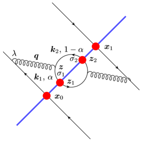
A

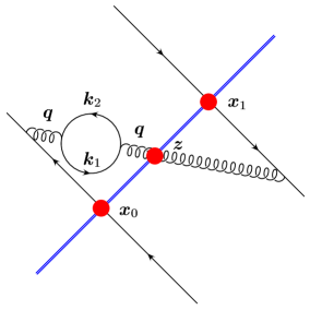
B

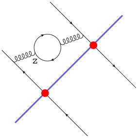
C

Figure 1: Diagrams giving the leading $\alpha_{s}N_{f}$ correction to the kernels of JIMWLK and BK small-$x$ evolution equations. The thick dots on gluon and quark lines denote interactions with the target.

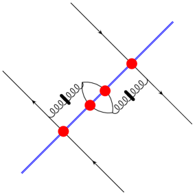
A^′

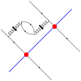
C^′

Figure 2: Diagrams with instantaneous parts of gluon propagators giving the leading $\alpha_{s}N_{f}$ correction to the kernels of JIMWLK and BK small-$x$ evolution equations. There is no analog of Fig. 1 B. All the lines are implied to be labeled in the same way as in Fig. 1.

To resum $\alpha_{s}N_{f}$ corrections we begin by considering the lowest order diagrams for one step of small-$x$ evolution containing a single quark bubble. These diagrams give the lowest order $\alpha_{s}N_{f}$ correction to the JIMWLK and/or BK evolution kernels and are shown in Fig. 1. The diagrams are time-ordered as they are drawn according to the rules of LCPT [41, 42]. Gluon lines in Figs. 1 A and C also have instantaneous/longitudinal counterparts [41, 42], shown in diagrams A^′ and C^′ in Fig. 2. (The virtual gluon on the left side of Fig. 1B can not be instantaneous, since the produced gluon on the right of Fig. 1B can only be transverse and a longitudinal gluon can not interfere with a transverse gluon, as will be seen in the calculations done below.)

2.1 Diagrams A and A^′

To calculate the forward scattering amplitude in Figs. 1A and 2A^′ we first need to calculate the wave function of a dipole emitting a gluon which then, in turn, splits into a quark–anti-quark pair, i.e., the part of the diagrams A and A^′ located on one side of the interaction with the target. The calculation is similar to what is presented in [45]. We will work in the $A_{+}=0$ light cone gauge in the framework of the light cone perturbation theory [41, 42, 46, 47]. The momentum space wave function of a dipole (or a single (anti-)quark) splitting into a gluon which in turn splits into a $q\bar{q}$ pair with the transverse momenta ${\bm{k}}_{1}$ and ${\bm{k}}_{2}$ of the quark and the anti-quark with the quark carrying a fraction $\alpha$ of the gluon’s longitudinal (“plus”) momentum is [45]

$$\Psi^{(1)}_{\sigma_{1},\,\sigma_{2}}(\bm{k}_{1},\bm{k}_{2},\alpha)\,=\,[t^{a}]_{\text{em}}\otimes[t^{a}]_{\text{f}}\,\psi^{(1)}_{\sigma_{1},\,\sigma_{2}}(\bm{k}_{1},\bm{k}_{2},\alpha)=-2\,g^{2}[t^{a}]_{\text{em}}\otimes[t^{a}]_{\text{f}}\sum\limits_{\lambda=\pm 1}\frac{{\bm{\epsilon}}^{*\lambda}\cdot({\bm{k}}_{1}+{\bm{k}}_{2})}{({\bm{k}}_{1}+{\bm{k}}_{2})^{2}}$$

$$\times\,\frac{{\bm{\epsilon}}^{\lambda}\cdot[{\bm{k}}_{1}(1-\alpha)-{\bm{k}}_{2}\alpha](1-2\alpha+\lambda\sigma_{1})\,\delta_{\sigma_{1}\sigma_{2}}}{{\bm{k}}_{1}^{2}(1-\alpha)+{\bm{k}}_{2}^{2}\alpha}-4\,g^{2}[t^{a}]_{\text{em}}\otimes[t^{a}]_{\text{f}}\,\frac{\alpha\,(1-\alpha)\,\delta_{\sigma_{1}\sigma_{2}}}{{\bm{k}}_{1}^{2}(1-\alpha)+{\bm{k}}_{2}^{2}\alpha}.$$ (3)

Here $\lambda=\pm 1$ is the internal gluon’s polarization: the gluon polarization vector for transverse gluons is given by $\epsilon_{\mu}^{\lambda}=(0,0,{\bm{\epsilon}}^{\lambda})$ with $\bm{\epsilon}^{\lambda}=(1+i\,\lambda)/\sqrt{2}$. The instantaneous diagram from Fig. 2A^′ gives the second term on the right hand side of Eq. (2.1). The produced quark and anti-quark are massless, which is sufficient for our purposes of determining the scale of the running coupling. $\sigma_{1}=\pm 1$ and $\sigma_{2}=\pm 1$ are quark and anti-quark helicities correspondingly (defined as in [45]). The fraction the of gluon’s “plus” momentum carried by the quark is denoted by $\alpha\equiv k_{1+}/(k_{1+}+k_{2+})$. The wave function also contains a color factor $[t^{a}]_{\text{em}}\otimes[t^{a}]_{\text{f}}$ consisting of two color matrices originating in the quark-gluon vertices at the points of emission of the gluon and its splitting into a $q\bar{q}$ pair.

It is convenient to rewrite Eq. (2.1) in terms of a different set of transverse momenta. Defining the momentum of the gluon ${\bm{q}}={\bm{k}}_{1}+{\bm{k}}_{2}$ and ${\bm{k}}={\bm{k}}_{1}(1-\alpha)-{\bm{k}}_{2}\alpha$, and noting that ${\bm{k}}_{1}^{2}(1-\alpha)+{\bm{k}}_{2}^{2}\alpha={\bm{k}}^{2}+{\bm{q}}^{2}\alpha(1-\alpha)$, we write

$$\psi^{(1)}_{\sigma_{1},\,\sigma_{2}}(\bm{k},\bm{q},\alpha)=-2\,g^{2}\,\sum\limits_{\lambda=\pm 1}\frac{{\bm{\epsilon}}^{*\lambda}\cdot{\bm{q}}}{{\bm{q}}^{2}}\frac{{\bm{\epsilon}}^{\lambda}\cdot{\bm{k}}\,(1-2\alpha+\lambda\sigma_{1})\,\delta_{\sigma_{1}\sigma_{2}}}{{\bm{k}}^{2}+{\bm{q}}^{2}\alpha(1-\alpha)}-4\,g^{2}\,\frac{\alpha\,(1-\alpha)\,\delta_{\sigma_{1}\sigma_{2}}}{{\bm{k}}^{2}+{\bm{q}}^{2}\alpha(1-\alpha)}.$$ (4)

Performing the summation over gluon polarizations $\lambda$ yields

$$\psi^{(1)}_{\sigma_{1},\,\sigma_{2}}(\bm{k},\bm{q},\alpha)=-2\,g^{2}\,\frac{{\bm{q}}_{i}}{{\bm{q}}^{2}}\,\left[(1-2\alpha)\delta_{ij}+i\sigma_{1}\epsilon_{ij}\right]\,\delta_{\sigma_{1}\sigma_{2}}\,\frac{{\bm{k}}_{j}}{{\bm{k}}^{2}+{\bm{q}}^{2}\alpha(1-\alpha)}-4\,g^{2}\,\frac{\alpha\,(1-\alpha)\,\delta_{\sigma_{1}\sigma_{2}}}{{\bm{k}}^{2}+{\bm{q}}^{2}\alpha(1-\alpha)}$$ (5)

where $q_{i}$ denotes the $i$th component of vector $\bm{q}$ and the sum over repeated indices $i,j=1,2$ is implied. Here $\epsilon_{12}=1=-\epsilon_{21}$, $\epsilon_{11}=\epsilon_{22}=0$, and, assuming summation over repeating indices, $\epsilon_{ij}\,q_{i}\,k_{j}=q_{x}\,k_{y}-q_{y}\,k_{x}$.

To find the contribution of the diagrams in Figs. 1A and 2A^′ to the next-to-leading order (NLO) evolution kernel we first have to transform the wave function from Eq. (5) into transverse coordinate space

$$\psi^{(1)}_{\sigma_{1},\,\sigma_{2}}({\bm{z}}_{1}-{\bm{x}}_{m},{\bm{z}}_{2}-{\bm{x}}_{m},\alpha)\,=\,\int\frac{d^{2}k_{1}}{(2\,\pi)^{2}}\,\frac{d^{2}k_{2}}{(2\,\pi)^{2}}\,e^{-i{\bm{k}}_{1}\cdot({\bm{z}}_{1}-{\bm{x}}_{m})-i{\bm{k}}_{2}\cdot({\bm{z}}_{2}-{\bm{x}}_{m})}\,\psi^{(1)}_{\sigma_{1},\,\sigma_{2}}(\bm{k}_{1},\bm{k}_{2},\alpha).$$ (6)

Here the transverse coordinates of the quark and the anti-quark are taken to be ${\bm{z}}_{1}$ and ${\bm{z}}_{2}$ correspondingly. The gluon in Fig. 1 can be emitted either off the quark or off the anti-quark in the incoming “parent” dipole. The transverse coordinates of the quark and the anti-quark in the “parent” dipole are ${\bm{x}}_{0}$ and ${\bm{x}}_{1}$. In Eq. (6) we labeled them ${\bm{x}}_{m}$ with $m=0,1$ depending on whether the gluon was emitted off the quark or off the anti-quark.

In terms of transverse momenta $\bm{k}$ and $\bm{q}$ Eq. (6) can be written as

$$\psi^{(1)}_{\sigma_{1},\,\sigma_{2}}({\bm{z}}_{1}-{\bm{x}}_{m},{\bm{z}}_{2}-{\bm{x}}_{m},\alpha)\,=\,\int\frac{d^{2}k}{(2\,\pi)^{2}}\,\frac{d^{2}q}{(2\,\pi)^{2}}\,e^{-i{\bm{k}}\cdot{\bm{z}}_{12}-i{\bm{q}}\cdot({\bm{z}}-{\bm{x}}_{m})}\,\psi^{(1)}_{\sigma_{1},\,\sigma_{2}}(\bm{k},\bm{q},\alpha),$$ (7)

where

$${\bm{z}}_{12}={\bm{z}}_{1}-{\bm{z}}_{2}$$ (8)

and

$${\bm{z}}=\alpha\,{\bm{z}}_{1}+(1-\alpha)\,{\bm{z}}_{2}$$ (9)

is the transverse position of the gluon.

Substituting the wave function from Eq. (5) into Eq. (7) and performing the integrations over $\bm{k}$ and $\bm{q}$ yields

$$\psi^{(1)}_{\sigma_{1},\,\sigma_{2}}({\bm{z}}_{1}-{\bm{x}}_{m},{\bm{z}}_{2}-{\bm{x}}_{m},\alpha)\,=\,2\,g^{2}\,\frac{1}{(2\pi)^{2}}\,\frac{({\bm{z}}-{\bm{x}}_{m})_{i}}{({\bm{z}}-{\bm{x}}_{m})^{2}+\alpha\,(1-\alpha)\,z_{12}^{2}}$$

$$\times\,\left[(1-2\alpha)\delta_{ij}+i\sigma_{1}\epsilon_{ij}\right]\,\delta_{\sigma_{1}\sigma_{2}}\,\frac{({\bm{z}}_{12})_{j}}{{\bm{z}}_{12}^{2}}-4\,g^{2}\,\frac{1}{(2\pi)^{2}}\,\frac{\alpha\,(1-\alpha)\,\delta_{\sigma_{1}\sigma_{2}}}{({\bm{z}}-{\bm{x}}_{m})^{2}+\alpha\,(1-\alpha)\,z_{12}^{2}}.$$ (10)

To calculate the diagram in Figs. 1A and 2A^′ using the wave function from Eq. (2.1) in a general case we have to include the interaction with the target by defining path-ordered exponential factors in the fundamental representation

$$U_{\bm{x}}\,=\,{\sf P}\exp\left[-ig\int\limits_{-\infty}^{\infty}\,dx_{+}\,A_{-}(x_{+},x_{-}=0,{\bm{x}})\right].$$ (11)

With the help of Eq. (11) we can write down

$$\parbox{65.44142pt}{\includegraphics[width=65.44142pt]{LoopInt-quarks-1-firsto}}+\parbox{65.44142pt}{\includegraphics[width=65.44142pt]{LoopInt-quarks-inst-1-firsto}}\,=$$

$$=\,\int d^{2}z_{1}d^{2}z_{2}\, \alpha_{\mu}^{2}\,{\cal K}_{1}^{\text{NLO}}({\bm{x}}_{0},{\bm{x}}_{1};{\bm{z}}_{1},{\bm{z}}_{2})\,U_{{\bm{x}}_{0}}t^{a}\otimes U_{{\bm{x}}_{1}}^{\dagger}t^{b}\ 2\,\text{tr}(t^{b}U_{{\bm{z}}_{1}}t^{a}U_{{\bm{z}}_{2}}^{\dagger})\,\ln(1/x_{\text{Bj}}),$$ (12)

where $x_{Bj}$ is the Bjorken $x$ variable. In arriving at Eq. (2.1) we have defined the NLO contribution to the JIMWLK kernel coming from the diagrams in Figs. 1A and 2A^′, labeled ${\cal K}_{1}^{\text{NLO}}$, by multiplying the wave function in Eq. (2.1) by its complex conjugate, summing the obtained expression over the helicities of the quark and the anti-quark in the produced pair and over $N_{f}$ quark flavors, and integrating over $\alpha$:

$$\alpha_{\mu}^{2}\,{\cal K}_{1}^{\text{NLO}}({\bm{x}}_{0},{\bm{x}}_{1};{\bm{z}}_{1},{\bm{z}}_{2})\,= \,\frac{N_{f}}{2\,(4\,\pi)^{2}}\,\int\limits_{0}^{1}d\alpha\sum_{\sigma_{1},\sigma_{2}=-1}^{1}$$

$$\times\,\psi^{(1)}_{\sigma_{1},\,\sigma_{2}}({\bm{z}}_{1}-{\bm{x}}_{0},{\bm{z}}_{2}-{\bm{x}}_{0},\alpha)\,\psi^{(1)*}_{\sigma_{1},\,\sigma_{2}}({\bm{z}}_{1}-{\bm{x}}_{1},{\bm{z}}_{2}-{\bm{x}}_{1},\alpha).$$ (13)

In this definition of ${\cal K}_{1}^{\text{NLO}}$ we use the wave function $\psi^{(1)}_{\sigma_{1},\,\sigma_{2}}$, which is different from the full wave function $\Psi^{(1)}_{\sigma_{1},\,\sigma_{2}}$ from Eq. (2.1) by the fact that the color matrices are included in $\Psi^{(1)}_{\sigma_{1},\,\sigma_{2}}$ and are not included in $\psi^{(1)}_{\sigma_{1},\,\sigma_{2}}$. We have used $\psi^{(1)}_{\sigma_{1},\,\sigma_{2}}$ to define the JIMWLK kernel ${\cal K}_{1}^{\text{NLO}}$ because the color matrices were already included in the forward amplitude in Eq. (2.1). A factor of $1/2$ was inserted in Eq. (2.1) to account for the factor of $2$ introduced in the definition of ${\cal K}_{1}^{\text{NLO}}$ in Eq. (2.1).

Substituting $\psi^{(1)}$ from Eq. (2.1) into Eq. (2.1) and summing over quark helicities yields

$${\cal K}_{1}^{\text{NLO}} ({\bm{x}}_{0},{\bm{x}}_{1};{\bm{z}}_{1},{\bm{z}}_{2})\,=\,\frac{N_{f}}{4\,\pi^{4}}\,\int\limits_{0}^{1}d\alpha$$

$$\times\,\Bigg{[}\frac{(1-2\alpha)^{2}{\bm{z}}_{12}\cdot({\bm{z}}-{\bm{x}}_{0})\ {\bm{z}}_{12}\cdot({\bm{z}}-{\bm{x}}_{1})+\epsilon_{ij}({\bm{z}}-{\bm{x}}_{0})_{i}({\bm{z}}_{12})_{j}\,\epsilon_{kl}({\bm{z}}-{\bm{x}}_{1})_{k}({\bm{z}}_{12})_{l}}{({\bm{z}}_{12}^{2})^{2}\,[({\bm{z}}-{\bm{x}}_{0})^{2}+\alpha\,(1-\alpha)\,z_{12}^{2}]\,[({\bm{z}}-{\bm{x}}_{1})^{2}+\alpha\,(1-\alpha)\,z_{12}^{2}]}$$

$$-2\,\alpha\,(1-\alpha)\,(1-2\alpha)\,\frac{{\bm{z}}_{12}\cdot({\bm{z}}-{\bm{x}}_{0})+{\bm{z}}_{12}\cdot({\bm{z}}-{\bm{x}}_{1})}{{\bm{z}}_{12}^{2}\,[({\bm{z}}-{\bm{x}}_{0})^{2}+\alpha\,(1-\alpha)\,z_{12}^{2}]\,[({\bm{z}}-{\bm{x}}_{1})^{2}+\alpha\,(1-\alpha)\,z_{12}^{2}]}$$

$$+\frac{4\,\alpha^{2}\,(1-\alpha)^{2}}{[({\bm{z}}-{\bm{x}}_{0})^{2}+\alpha\,(1-\alpha)\,z_{12}^{2}]\,[({\bm{z}}-{\bm{x}}_{1})^{2}+\alpha\,(1-\alpha)\,z_{12}^{2}]}\Bigg{]}.$$ (14)

The integral over longitudinal momentum fraction $\alpha$, while straightforward to perform, would not make the above expression any more transparent. When squaring $\psi^{(1)}$ from Eq. (2.1) one gets a cross-product between the first and the second terms on the right hand side of Eq. (2.1), given by the second term in the square brackets of Eq. (2.1). Terms like that are also present in other physical quantities, such as the $q\bar{q}$ production cross section calculated in [45].

To obtain the contribution of the diagrams in Figs. 1A and 2A^′ to the BK evolution kernel $K_{1}^{\text{NLO}}$ we have to sum the wave function $\Psi^{(1)}_{\sigma_{1},\,\sigma_{2}}$ over all possible emissions of the gluon off the quark and off the anti-quark, multiply the result by its complex conjugate, sum over quark and anti-quark helicities and $N_{f}$ quark flavors, take a trace over color indices averaging over $N_{c}$ colors of the incoming dipole and integrate over $\alpha$

$$\alpha_{\mu}^{2}\,K_{1}^{\text{NLO}}({\bm{x}}_{0},{\bm{x}}_{1};{\bm{z}}_{1},{\bm{z}}_{2})\,= \,\frac{N_{f}}{(4\,\pi)^{2}}\,\int\limits_{0}^{1}d\alpha\sum_{\sigma_{1},\sigma_{2}=-1}^{1}\sum_{m,n=0}^{1}\,(-1)^{m+n}$$

$$\times\, \frac{1}{N_{c}}\,\ \text{tr}\left[\Psi^{(1)}_{\sigma_{1},\,\sigma_{2}}({\bm{z}}_{1}-{\bm{x}}_{0},{\bm{z}}_{2}-{\bm{x}}_{0},\alpha)\,\Psi^{(1)*}_{\sigma_{1},\,\sigma_{2}}({\bm{z}}_{1}-{\bm{x}}_{1},{\bm{z}}_{2}-{\bm{x}}_{1},\alpha)\right].$$ (15)

(Note that the capital $K$ denotes the kernel of the BK evolution equation, while the calligraphic $\cal K$ is reserved for the JIMWLK evolution kernel.) Using the first line of Eq. (2.1) along with Eq. (2.1) in Eq. (2.1) one can show that

$$K_{1}^{\text{NLO}}({\bm{x}}_{0},{\bm{x}}_{1};{\bm{z}}_{1},{\bm{z}}_{2})\,=\,C_{F}\,\sum_{m,n=0}^{1}\,(-1)^{m+n}\,{\cal K}_{1}^{\text{NLO}} ({\bm{x}}_{m},{\bm{x}}_{n};{\bm{z}}_{1},{\bm{z}}_{2}).$$ (16)

For the reasons which will become apparent momentarily, it is more convenient to leave ${\cal K}^{\text{NLO}}_{1}$ written in terms of integrals in transverse momentum space. Using Eqs. (5), (7) in Eq. (2.1) and summing over quark helicities yields

$${\cal K}_{1}^{\text{NLO}}({\bm{x}}_{0},{\bm{x}}_{1};{\bm{z}}_{1},{\bm{z}}_{2})\,= \,4\,N_{f}\,\int\limits_{0}^{1}d\alpha\,\int\frac{d^{2}k}{(2\pi)^{2}}\frac{d^{2}k^{\prime}}{(2\pi)^{2}}\frac{d^{2}q}{(2\pi)^{2}}\frac{d^{2}q^{\prime}}{(2\pi)^{2}}\ e^{-i{\bm{q}}\cdot({\bm{z}}-{\bm{x}}_{0})+i{\bm{q}}^{\prime}\cdot({\bm{z}}-{\bm{x}}_{1})-i({\bm{k}}-{\bm{k}}^{\prime})\cdot{\bm{z}}_{12}}$$

$$\times\left[\frac{1}{{\bm{q}}^{2}{\bm{q}}^{\prime 2}}\frac{(1-2\alpha)^{2}{\bm{q}}\cdot{\bm{k}}\ {\bm{k}}^{\prime}\cdot{\bm{q}}^{\prime}+{\bm{q}}\cdot{\bm{q}}^{\prime}\ {\bm{k}}\cdot{\bm{k}}^{\prime}-{\bm{q}}\cdot{\bm{k}}^{\prime}\ {\bm{k}}\cdot{\bm{q}}^{\prime}}{\Big{[}{\bm{k}}^{2}+{\bm{q}}^{2}\alpha(1-\alpha)\Big{]}\Big{[}{\bm{k}}^{\prime 2}+{\bm{q}}^{\prime 2}\alpha(1-\alpha)\Big{]}}\right.$$

$$+\frac{2\,\alpha\,(1-\alpha)\,(1-2\alpha)}{\Big{[}{\bm{k}}^{2}+{\bm{q}}^{2}\alpha(1-\alpha)\Big{]}\Big{[}{\bm{k}}^{\prime 2}+{\bm{q}}^{\prime 2}\alpha(1-\alpha)\Big{]}}\,\left(\frac{{\bm{k}}\cdot{\bm{q}}}{{\bm{q}}^{2}}+\frac{{\bm{k}}^{\prime}\cdot{\bm{q}}^{\prime}}{{\bm{q}}^{\prime 2}}\right)$$

$$\left.+\,\frac{4\,\alpha^{2}\,(1-\alpha)^{2}}{\Big{[}{\bm{k}}^{2}+{\bm{q}}^{2}\alpha(1-\alpha)\Big{]}\Big{[}{\bm{k}}^{\prime 2}+{\bm{q}}^{\prime 2}\alpha(1-\alpha)\Big{]}}\right],$$ (17)

where we have used the identity

$$\epsilon_{ij}\,{\bm{q}}_{i}\,{\bm{k}}_{j}\ \epsilon_{kl}\,{\bm{q}}^{\prime}_{k}\,{\bm{k}}^{\prime}_{l}={\bm{q}}\cdot{\bm{q}}^{\prime}\ {\bm{k}}\cdot{\bm{k}}^{\prime}-{\bm{q}}\cdot{\bm{k}}^{\prime}\ {\bm{k}}\cdot{\bm{q}}^{\prime}.$$ (18)

2.2 Diagram B

Unlike the diagram A, the diagram B in Fig. 1 looks more like a “typical” running coupling correction to the leading order JIMWLK/BK kernels. The contribution of the diagram B along with its mirror-reflection with respect to the line denoting the interaction with the target can be written as

$$\parbox{65.44142pt}{\includegraphics[width=65.44142pt]{LoopInt-glue-1-firsto-left}}+\parbox{65.44142pt}{\includegraphics[width=65.44142pt]{LoopInt-glue-1-firsto-right}}\,=\,\int d^{2}z\ \alpha_{\mu}^{2}\,{\cal K}_{2}^{\text{NLO}}({\bm{x}}_{0},{\bm{x}}_{1};{\bm{z}})\ U_{{\bm{x}}_{0}}t^{a}\otimes U_{{\bm{x}}_{1}}^{\dagger}t^{b}\ U^{ab}_{\bm{z}}\ \ln(1/x_{\text{Bj}})$$ (19)

with the corresponding NLO contribution ${\cal K}_{2}^{\text{NLO}}$ to the JIMWLK kernel calculated using the rules of the light-cone perturbation theory [41, 42]. We first decompose the kernel ${\cal K}_{2}^{\text{NLO}}$ into a sum of the contributions of the diagram Fig. 1B (denoted ${\cal K}_{2\,\text{left}}^{\text{NLO}}$) and its mirror-image (denoted ${\cal K}_{2\,\text{right}}^{\text{NLO}}$):

$${\cal K}_{2}^{\text{NLO}}({\bm{x}}_{0},{\bm{x}}_{1};{\bm{z}})\,=\,{\cal K}_{2\,\text{left}}^{\text{NLO}}({\bm{x}}_{0},{\bm{x}}_{1};{\bm{z}})+{\cal K}_{2\,\text{right}}^{\text{NLO}}({\bm{x}}_{0},{\bm{x}}_{1};{\bm{z}}).$$ (20)

Below we will only calculate ${\cal K}_{2\,\text{left}}^{\text{NLO}}$: to construct ${\cal K}_{2\,\text{right}}^{\text{NLO}}$ one only has to replace ${\bm{x}}_{0}\leftrightarrow{\bm{x}}_{1}$ in its argument. A simple calculation along the same lines as the calculation of the diagram A done above yields

$$\alpha_{\mu}^{2}\,{\cal K}_{2\,\text{left}}^{\text{NLO}}({\bm{x}}_{0},{\bm{x}}_{1};{\bm{z}})\,=\,\frac{N_{f}}{(4\,\pi)^{2}}\,2\,g^{4}\,\int\limits_{0}^{1}\frac{d\alpha}{\alpha(1-\alpha)}\,\int\frac{d^{2}k}{(2\pi)^{2}}\frac{d^{2}q}{(2\pi)^{2}}\frac{d^{2}q^{\prime}}{(2\pi)^{2}}\ e^{-i{\bm{q}}\cdot({\bm{z}}-{\bm{x}}_{0})+i{\bm{q}}^{\prime}\cdot({\bm{z}}-{\bm{x}}_{1})}$$

$$\sum_{\sigma_{1},\sigma_{2}=-1}^{1}\,\sum_{\lambda,\lambda^{\prime}=-1}^{1}\,\frac{{\bm{\epsilon}}^{*\lambda}\cdot{\bm{q}}}{{\bm{q}}^{2}}\frac{{\bm{\epsilon}}^{\lambda}\cdot{\bm{k}}\,(1-2\alpha+\lambda\sigma_{1})\delta_{\sigma_{1}\sigma_{2}}}{{\bm{k}}^{2}+{\bm{q}}^{2}\alpha(1-\alpha)}\,\frac{{\bm{\epsilon}}^{*\lambda^{\prime}}\cdot{\bm{k}}\,(1-2\alpha+\lambda^{\prime}\sigma_{1})}{{\bm{q}}^{2}}\,\frac{{\bm{\epsilon}}^{\lambda^{\prime}}\cdot{\bm{q}}^{\prime}}{{\bm{q}}^{\prime 2}}$$ (21)

with all the notation being the same as in the case of the diagram 1A and $\lambda^{\prime}=\pm 1$ the polarization of the gluon interacting with the target. Different from ${\cal K}_{1}^{\text{NLO}}$, the kernel ${\cal K}_{2\,\text{left}}^{\text{NLO}}$ in Eq. (2.2) has a part of the color factor included in it: it includes of $1/2$ coming from the color trace of the quark loop, which is required by the definition of ${\cal K}_{2}^{\text{NLO}}$ in Eq. (19). Similar to the above, to obtain the corresponding correction to the BK evolution kernel, we use

$$K_{2}^{\text{NLO}}({\bm{x}}_{0},{\bm{x}}_{1};{\bm{z}})\,=\,C_{F}\,\sum_{m,n=0}^{1}\,(-1)^{m+n}\,{\cal K}_{2}^{\text{NLO}} ({\bm{x}}_{m},{\bm{x}}_{n};{\bm{z}})$$ (22)

[Similar relationships holds for for both ${\cal K}_{2\,\text{left}}^{\text{NLO}}$ and ${\cal K}_{2\,\text{right}}^{\text{NLO}}$ separately.]

We can simplify Eq. (2.2). First we sum over the quark helicities and gluon polarizations to obtain

$${\cal K}_{2\,\text{left}}^{\text{NLO}}({\bm{x}}_{0},{\bm{x}}_{1};{\bm{z}})\,=\,4\,N_{f}\,\int\limits_{0}^{1}\frac{d\alpha}{\alpha(1-\alpha)}\,\int\frac{d^{d}k}{(2\pi)^{d}}\frac{d^{2}q}{(2\pi)^{2}}\frac{d^{2}q^{\prime}}{(2\pi)^{2}}\ e^{-i{\bm{q}}\cdot({\bm{z}}-{\bm{x}}_{0})+i{\bm{q}}^{\prime}\cdot({\bm{z}}-{\bm{x}}_{1})}$$

$$\times\,\frac{(1-2\alpha)^{2}{\bm{q}}\cdot{\bm{k}}\ {\bm{k}}\cdot{\bm{q}}^{\prime}+{\bm{q}}\cdot{\bm{q}}^{\prime}\ {\bm{k}}^{2}-{\bm{q}}\cdot{\bm{k}}\ {\bm{k}}\cdot{\bm{q}}^{\prime}}{({\bm{q}}^{2})^{2}\,{\bm{q}}^{\prime 2}\,\Big{[}{\bm{k}}^{2}+{\bm{q}}^{2}\alpha(1-\alpha)\Big{]}}.$$ (23)

The integral over $\bm{k}$ is UV-divergent, as expected. We will regularize it by using dimensional regularization, for which purpose we have replaced $d^{2}k/(2\pi)^{2}\rightarrow d^{d}k/(2\pi)^{d}$ in Eq. (22) with $d$ the number of dimensions. Anticipating the integration over the angles of the vector $\bm{k}$ we also replace

$${\bm{k}}_{i}\,{\bm{k}}_{j}\,\rightarrow\,\frac{{\bm{k}}^{2}}{d}\,\delta_{ij}$$ (24)

in Eq. (2.2), obtaining

$${\cal K}_{2\,\text{left}}^{\text{NLO}}({\bm{x}}_{0},{\bm{x}}_{1};{\bm{z}})\,=\,4\,N_{f}\,\int\limits_{0}^{1}\frac{d\alpha}{\alpha(1-\alpha)}\,\int\frac{d^{2}q}{(2\pi)^{2}}\frac{d^{2}q^{\prime}}{(2\pi)^{2}}\ e^{-i{\bm{q}}\cdot({\bm{z}}-{\bm{x}}_{0})+i{\bm{q}}^{\prime}\cdot({\bm{z}}-{\bm{x}}_{1})}\,\frac{{\bm{q}}\cdot{\bm{q}}^{\prime}}{({\bm{q}}^{2})^{2}\,{\bm{q}}^{\prime 2}}$$

$$\times\,\frac{1}{d}\,\int\frac{d^{d}k}{(2\pi)^{d}}\frac{{\bm{k}}^{2}}{{\bm{k}}^{2}+{\bm{q}}^{2}\alpha(1-\alpha)}\,\left[(1-2\alpha)^{2}+d-1\right].$$ (25)

Now the $\bm{k}$-integral is easily doable (see, e.g., [48]) yielding

$${\cal K}_{2\,\text{left}}^{\text{NLO}}({\bm{x}}_{0},{\bm{x}}_{1};{\bm{z}})\,=\,4\,N_{f}\,\int\limits_{0}^{1}\frac{d\alpha}{\alpha(1-\alpha)}\,\int\frac{d^{2}q}{(2\pi)^{2}}\frac{d^{2}q^{\prime}}{(2\pi)^{2}}\ e^{-i{\bm{q}}\cdot({\bm{z}}-{\bm{x}}_{0})+i{\bm{q}}^{\prime}\cdot({\bm{z}}-{\bm{x}}_{1})}\,\frac{{\bm{q}}\cdot{\bm{q}}^{\prime}}{({\bm{q}}^{2})^{2}\,{\bm{q}}^{\prime 2}}$$

$$\times\,\frac{1}{2\,(4\pi)^{d/2}}\,\Gamma\left(-\frac{d}{2}\right)\,\left[{\bm{q}}^{2}\alpha(1-\alpha)\right]^{d/2}\,\left[(1-2\alpha)^{2}+d-1\right].$$ (26)

Writing $d=2-\epsilon$ and expanding around $\epsilon=0$ we get

$${\cal K}_{2\,\text{left}}^{\text{NLO}}({\bm{x}}_{0},{\bm{x}}_{1};{\bm{z}})\,=\,\frac{N_{f}}{2\,\pi}\,\int\limits_{0}^{1}d\alpha\,\int\frac{d^{2}q}{(2\pi)^{2}}\frac{d^{2}q^{\prime}}{(2\pi)^{2}}\ e^{-i{\bm{q}}\cdot({\bm{z}}-{\bm{x}}_{0})+i{\bm{q}}^{\prime}\cdot({\bm{z}}-{\bm{x}}_{1})}\,\frac{{\bm{q}}\cdot{\bm{q}}^{\prime}}{{\bm{q}}^{2}\,{\bm{q}}^{\prime 2}}$$

$$\times\,\left\{\left[(1-2\alpha)^{2}+1\right]\,\left[\ln\frac{{\bm{q}}^{2}\,\alpha\,(1-\alpha)}{\mu_{{\text{MS}}}^{2}}+\gamma-\ln 4\pi-1\right]+2\right\},$$ (27)

where we replaced $1/\epsilon$ with $\ln\mu_{{\text{MS}}}$. Integrating over $\alpha$ we obtain

$${\cal K}_{2\,\text{left}}^{\text{NLO}}({\bm{x}}_{0},{\bm{x}}_{1};{\bm{z}})\,=\,\frac{2\,N_{f}}{3\,\pi}\,\int\frac{d^{2}q}{(2\pi)^{2}}\frac{d^{2}q^{\prime}}{(2\pi)^{2}}\ e^{-i{\bm{q}}\cdot({\bm{z}}-{\bm{x}}_{0})+i{\bm{q}}^{\prime}\cdot({\bm{z}}-{\bm{x}}_{1})}\,\frac{{\bm{q}}\cdot{\bm{q}}^{\prime}}{{\bm{q}}^{2}\,{\bm{q}}^{\prime 2}}\,\left\{\ln\frac{{\bm{q}}^{2}}{\mu_{\overline{{\text{MS}}}}^{2}}-\frac{5}{3}\right\}$$ (28)

with $\mu_{\overline{{\text{MS}}}}^{2}=\mu_{{\text{MS}}}^{2}\,4\pi\,e^{-\gamma}$.

While Eq. (28) is sufficiently simple for our later purposes, we can further simplify it by Fourier-transforming it into transverse coordinate space. A straightforward integration yields the NLO contribution to the JIMWLK kernel coming from the diagram B

$${\cal K}_{2\,\text{left}}^{\text{NLO}}({\bm{x}}_{0},{\bm{x}}_{1};{\bm{z}})\,=\,\frac{N_{f}}{6\,\pi^{3}}\,\frac{{\bm{z}}-{\bm{x}}_{0}}{|{\bm{z}}-{\bm{x}}_{0}|^{2}}\cdot\frac{{\bm{z}}-{\bm{x}}_{1}}{|{\bm{z}}-{\bm{x}}_{1}|^{2}}\,\left\{\ln\frac{4}{|{\bm{z}}-{\bm{x}}_{0}|^{2}\,\mu_{\overline{{\text{MS}}}}^{2}}-\frac{5}{3}-2\gamma\right\}.$$ (29)

Similarly one can show that

$${\cal K}_{2\,\text{right}}^{\text{NLO}}({\bm{x}}_{0},{\bm{x}}_{1};{\bm{z}})\,=\,\frac{N_{f}}{6\,\pi^{3}}\,\frac{{\bm{z}}-{\bm{x}}_{0}}{|{\bm{z}}-{\bm{x}}_{0}|^{2}}\cdot\frac{{\bm{z}}-{\bm{x}}_{1}}{|{\bm{z}}-{\bm{x}}_{1}|^{2}}\,\left\{\ln\frac{4}{|{\bm{z}}-{\bm{x}}_{1}|^{2}\,\mu_{\overline{{\text{MS}}}}^{2}}-\frac{5}{3}-2\gamma\right\}$$ (30)

and

$${\cal K}_{2}^{\text{NLO}}({\bm{x}}_{0},{\bm{x}}_{1};{\bm{z}})\,= \,{\cal K}_{2\,\text{left}}^{\text{NLO}}({\bm{x}}_{0},{\bm{x}}_{1};{\bm{z}})+{\cal K}_{2\,\text{right}}^{\text{NLO}}({\bm{x}}_{0},{\bm{x}}_{1};{\bm{z}})$$

$$\,= \,\frac{N_{f}}{6\,\pi^{3}}\,\frac{{\bm{z}}-{\bm{x}}_{0}}{|{\bm{z}}-{\bm{x}}_{0}|^{2}}\cdot\frac{{\bm{z}}-{\bm{x}}_{1}}{|{\bm{z}}-{\bm{x}}_{1}|^{2}}\,\left\{\ln\frac{4\,e^{-\frac{5}{3}-2\gamma}}{|{\bm{z}}-{\bm{x}}_{0}|^{2}\,\mu_{\overline{{\text{MS}}}}^{2}}+\ln\frac{4\,e^{-\frac{5}{3}-2\gamma}}{|{\bm{z}}-{\bm{x}}_{1}|^{2}\,\mu_{\overline{{\text{MS}}}}^{2}}\right\}.$$ (31)

The corresponding contribution to the NLO BK kernel can be easily obtained from Eq. (2.2) using Eq. (22).

Recalling that the leading order (LO) JIMWLK kernel is given by

$${\cal K}^{\text{LO}}({\bm{x}}_{0},{\bm{x}}_{1};{\bm{z}})\,=\,\frac{1}{\pi^{2}}\,\frac{{\bm{z}}-{\bm{x}}_{0}}{|{\bm{z}}-{\bm{x}}_{0}|^{2}}\cdot\frac{{\bm{z}}-{\bm{x}}_{1}}{|{\bm{z}}-{\bm{x}}_{1}|^{2}}$$ (32)

we immediately see that adding ${\cal K}_{2}^{\text{NLO}}$ from Eq. (2.2) to it yields

$$\alpha_{\mu}\,{\cal K}^{LO}({\bm{x}}_{0},{\bm{x}}_{1};{\bm{z}})+\alpha_{\mu}^{2}\,{\cal K}_{2}^{\text{NLO}}({\bm{x}}_{0},{\bm{x}}_{1};{\bm{z}})\,=\,\frac{\alpha_{\mu}}{\pi^{2}}\,\frac{{\bm{z}}-{\bm{x}}_{0}}{|{\bm{z}}-{\bm{x}}_{0}|^{2}}\cdot\frac{{\bm{z}}-{\bm{x}}_{1}}{|{\bm{z}}-{\bm{x}}_{1}|^{2}}$$

$$\times\,\left\{1+\frac{\alpha_{\mu}\,N_{f}}{6\,\pi}\,\left[\ln\frac{4\,e^{-\frac{5}{3}-2\gamma}}{|{\bm{z}}-{\bm{x}}_{0}|^{2}\,\mu_{\overline{{\text{MS}}}}^{2}}+\ln\frac{4\,e^{-\frac{5}{3}-2\gamma}}{|{\bm{z}}-{\bm{x}}_{1}|^{2}\,\mu_{\overline{{\text{MS}}}}^{2}}\right]\right\}.$$ (33)

Anticipating the appearance of the full QCD beta-function we perform the replacement of Eq. (1) in Eq. (2.2) to obtain

$$\alpha_{\mu}\,{\cal K}^{LO}({\bm{x}}_{0},{\bm{x}}_{1};{\bm{z}})+\alpha_{\mu}^{2}\,{\cal K}_{2}^{\text{NLO}}({\bm{x}}_{0},{\bm{x}}_{1};{\bm{z}})\,=\,\frac{\alpha_{\mu}}{\pi^{2}}\,\frac{{\bm{z}}-{\bm{x}}_{0}}{|{\bm{z}}-{\bm{x}}_{0}|^{2}}\cdot\frac{{\bm{z}}-{\bm{x}}_{1}}{|{\bm{z}}-{\bm{x}}_{1}|^{2}}$$

$$\times\,\left\{1-\alpha_{\mu}\,\beta_{2}\,\left[\ln\frac{4\,e^{-\frac{5}{3}-2\gamma}}{|{\bm{z}}-{\bm{x}}_{0}|^{2}\,\mu_{\overline{{\text{MS}}}}^{2}}+\ln\frac{4\,e^{-\frac{5}{3}-2\gamma}}{|{\bm{z}}-{\bm{x}}_{1}|^{2}\,\mu_{\overline{{\text{MS}}}}^{2}}\right]\right\}.$$ (34)

Now one can readily see that the diagram B in Fig. 1 gives a contribution to the one-loop running coupling correction to the LO JIMWLK and BK kernels, as expected.

2.3 Diagrams C and C^′

The contribution of the diagrams in Figs. 1C and 2C^′ along with their mirror-reflections can be written as

$$\parbox{65.44142pt}{\includegraphics[width=65.44142pt]{LoopNonInt-up-to-1-firsto}}+\parbox{65.44142pt}{\includegraphics[width=65.44142pt]{LoopNonInt-down-to-1-firsto}}+\parbox{65.44142pt}{\includegraphics[width=65.44142pt]{LoopNonInt-up-to-inst-1-firsto}}+\parbox{65.44142pt}{\includegraphics[width=65.44142pt]{LoopNonInt-down-to-inst-1-firsto}}\,=$$

$$=\,\int d^{2}z\ \alpha_{\mu}^{2}\,{\cal K}_{3}^{\text{NLO}}({\bm{x}}_{0},{\bm{x}}_{1};{\bm{z}})\ U_{{\bm{x}}_{0}}t^{a}\otimes U_{{\bm{x}}_{1}}^{\dagger}t^{a}\ \ln(1/x_{\text{Bj}})$$ (35)

where $\bm{z}$ is still the gluon’s transverse coordinate which we choose to keep explicitly even though, since both gluon lines are now completely virtual, they do not interact with the target. Instead of calculating the NLO correction to the JIMWLK kernel ${\cal K}_{3}^{\text{NLO}}$ coming from the diagrams C and C^′ explicitly we will use the conservation of probability condition, which states that, in the absence of interaction with the target, the sum of all three diagrams in Fig. 1 (along with the mirror images of the diagrams B and C reflected with respect to the line representing the interaction with the target) gives zero. Intuitively this condition is clear: in the absence of interactions there will be no contribution to the evolution kernel. In the diagrammatic sense, adding up all the graphs in Fig. 1 corresponds to summing over all the cuts for the diagram of the gluon emission with a quark bubble correction. Similarly, if the interactions are absent, the sum of the diagrams in Fig. 2 along with the mirror-reflection of the diagram C^′ also gives zero. This probability conservation condition was originally used by Mueller to calculate the virtual correction to the leading order gluon emission in the dipole evolution kernel in [22]. In our case it formally reads

$$\int d^{2}z_{1}d^{2}z_{2}\ {\cal K}_{1}^{\text{NLO}}({\bm{x}}_{0},{\bm{x}}_{1};{\bm{z}}_{1},{\bm{z}}_{2})+\int d^{2}z\ {\cal K}_{2}^{\text{NLO}}({\bm{x}}_{0},{\bm{x}}_{1};{\bm{z}})+\int d^{2}z\ {\cal K}_{3}^{\text{NLO}}({\bm{x}}_{0},{\bm{x}}_{1};{\bm{z}})\,=\,0.$$ (36)

Noting that

$$d^{2}z_{1}\,d^{2}z_{2}\,=\,d^{2}z\,d^{2}z_{12}$$ (37)

with ${\bm{z}}_{12}$ and $\bm{z}$ defined in Eqs. (8) and (9) above, an explicit diagram calculation (keeping all the transverse momenta fixed in momentum space) yields an even stronger identity than Eq. (36):

$${\cal K}_{3}^{\text{NLO}}({\bm{x}}_{0},{\bm{x}}_{1};{\bm{z}})\,=\,-\int d^{2}z_{12}\ {\cal K}_{1}^{\text{NLO}}({\bm{x}}_{0},{\bm{x}}_{1};{\bm{z}}_{1},{\bm{z}}_{2})-\ {\cal K}_{2}^{\text{NLO}}({\bm{x}}_{0},{\bm{x}}_{1};{\bm{z}}).$$ (38)

${\cal K}_{2}^{\text{NLO}}$ in Eq. (38) is given explicitly in Eq. (2.2). Using the momentum-space expression (2.1) for ${\cal K}_{1}^{\text{NLO}}$ we get

$$\int d^{2}z_{12}\,{\cal K}_{1}^{\text{NLO}}({\bm{x}}_{0},{\bm{x}}_{1};{\bm{z}}_{1},{\bm{z}}_{2})\,= \,4\,N_{f}\,\int\limits_{0}^{1}d\alpha\,\int\frac{d^{d}k}{(2\pi)^{d}}\frac{d^{2}q}{(2\pi)^{2}}\frac{d^{2}q^{\prime}}{(2\pi)^{2}}\ e^{-i{\bm{q}}\cdot({\bm{z}}-{\bm{x}}_{0})+i{\bm{q}}^{\prime}\cdot({\bm{z}}-{\bm{x}}_{1})}$$

$$\times\left[\frac{1}{{\bm{q}}^{2}{\bm{q}}^{\prime 2}}\frac{(1-2\alpha)^{2}{\bm{q}}\cdot{\bm{k}}\ {\bm{k}}\cdot{\bm{q}}^{\prime}+{\bm{q}}\cdot{\bm{q}}^{\prime}\ {\bm{k}}^{2}-{\bm{q}}\cdot{\bm{k}}\ {\bm{k}}\cdot{\bm{q}}^{\prime}}{\Big{[}{\bm{k}}^{2}+{\bm{q}}^{2}\alpha(1-\alpha)\Big{]}\Big{[}{\bm{k}}^{2}+{\bm{q}}^{\prime 2}\alpha(1-\alpha)\Big{]}}\right.$$

$$+\,\left.\frac{4\,\alpha^{2}\,(1-\alpha)^{2}}{\Big{[}{\bm{k}}^{2}+{\bm{q}}^{2}\alpha(1-\alpha)\Big{]}\Big{[}{\bm{k}}^{2}+{\bm{q}}^{\prime 2}\alpha(1-\alpha)\Big{]}}\right],$$ (39)

where the $\bm{k}$-integral is UV-divergent, which we regularize using dimensional regularization. With the help of Eq. (24) we rewrite Eq. (2.3) as

$$\int d^{2}z_{12}\,{\cal K}_{1}^{\text{NLO}}({\bm{x}}_{0},{\bm{x}}_{1};{\bm{z}}_{1},{\bm{z}}_{2})\,=\,4\,N_{f}\,\int\limits_{0}^{1}d\alpha\,\int\frac{d^{2}q}{(2\pi)^{2}}\frac{d^{2}q^{\prime}}{(2\pi)^{2}}\ e^{-i{\bm{q}}\cdot({\bm{z}}-{\bm{x}}_{0})+i{\bm{q}}^{\prime}\cdot({\bm{z}}-{\bm{x}}_{1})}$$

$$\times\,\Bigg{\{}\frac{{\bm{q}}\cdot{\bm{q}}^{\prime}}{{\bm{q}}^{2}{\bm{q}}^{\prime 2}}\,\frac{1}{d}\,\int\frac{d^{d}k}{(2\pi)^{d}}\,\frac{{\bm{k}}^{2}}{\Big{[}{\bm{k}}^{2}+{\bm{q}}^{2}\alpha(1-\alpha)\Big{]}\Big{[}{\bm{k}}^{2}+{\bm{q}}^{\prime 2}\alpha(1-\alpha)\Big{]}}\,\left[(1-2\alpha)^{2}+d-1\right]$$

$$+\,4\,\alpha^{2}\,(1-\alpha)^{2}\,\int\frac{d^{2}k}{(2\pi)^{2}}\,\frac{1}{\Big{[}{\bm{k}}^{2}+{\bm{q}}^{2}\alpha(1-\alpha)\Big{]}\Big{[}{\bm{k}}^{2}+{\bm{q}}^{\prime 2}\alpha(1-\alpha)\Big{]}}\Bigg{\}},$$ (40)

where we put $d=2$ in the second term in the curly brackets since the integral in that term is not divergent. Performing the $\bm{k}$-integrals yields

$$\int d^{2}z_{12}\,{\cal K}_{1}^{\text{NLO}}({\bm{x}}_{0},{\bm{x}}_{1};{\bm{z}}_{1},{\bm{z}}_{2})\,=\,4\,N_{f}\,\int\limits_{0}^{1}d\alpha\,\int\frac{d^{2}q}{(2\pi)^{2}}\frac{d^{2}q^{\prime}}{(2\pi)^{2}}\ e^{-i{\bm{q}}\cdot({\bm{z}}-{\bm{x}}_{0})+i{\bm{q}}^{\prime}\cdot({\bm{z}}-{\bm{x}}_{1})}$$

$$\times\,\Bigg{\{}\frac{{\bm{q}}\cdot{\bm{q}}^{\prime}}{{\bm{q}}^{2}{\bm{q}}^{\prime 2}}\frac{1}{d}\,\frac{1}{(4\,\pi)^{d/2}}\,\Gamma\left(1-\frac{d}{2}\right)\,[\alpha\,(1-\alpha)]^{\frac{d}{2}-1}\,\left[(1-2\alpha)^{2}+d-1\right]\,\frac{[{\bm{q}}^{2}]^{d/2}-[{\bm{q}}^{\prime 2}]^{d/2}}{{\bm{q}}^{2}-{\bm{q}}^{\prime 2}}$$

$$+\,\frac{1}{\pi}\,\alpha\,(1-\alpha)\,\frac{\ln({\bm{q}}^{2}/{\bm{q}}^{\prime 2})}{{\bm{q}}^{2}-{\bm{q}}^{\prime 2}}\Bigg{\}}.$$ (41)

Writing $d=2-\epsilon$, expanding around $\epsilon=0$, replacing $1/\epsilon$ with $\ln\mu_{{\text{MS}}}$ and integrating over $\alpha$ we obtain

$$\int d^{2}z_{12}\,{\cal K}_{1}^{\text{NLO}}({\bm{x}}_{0},{\bm{x}}_{1};{\bm{z}}_{1},{\bm{z}}_{2})\,=\,-\frac{2\,N_{f}}{3\,\pi}\,\int\frac{d^{2}q}{(2\pi)^{2}}\frac{d^{2}q^{\prime}}{(2\pi)^{2}}\ e^{-i{\bm{q}}\cdot({\bm{z}}-{\bm{x}}_{0})+i{\bm{q}}^{\prime}\cdot({\bm{z}}-{\bm{x}}_{1})}$$

$$\times\,\Bigg{\{}\frac{{\bm{q}}\cdot{\bm{q}}^{\prime}}{{\bm{q}}^{2}{\bm{q}}^{\prime 2}}\,\frac{{\bm{q}}^{2}\,\left(\ln\frac{{\bm{q}}^{2}}{\mu_{\overline{{\text{MS}}}}^{2}}-\frac{5}{3}\right)-{\bm{q}}^{\prime 2}\,\left(\ln\frac{{\bm{q}}^{\prime 2}}{\mu_{\overline{{\text{MS}}}}^{2}}-\frac{5}{3}\right)}{{\bm{q}}^{2}-{\bm{q}}^{\prime 2}}-\frac{\ln({\bm{q}}^{2}/{\bm{q}}^{\prime 2})}{{\bm{q}}^{2}-{\bm{q}}^{\prime 2}}\Bigg{\}}.$$ (42)

The details of integrations over $\bm{q}$ and ${\bm{q}}^{\prime}$ are shown in Appendix A. The result reads

$$\int d^{2}z_{12}\,{\cal K}_{1}^{\text{NLO}}({\bm{x}}_{0},{\bm{x}}_{1};{\bm{z}}_{1},{\bm{z}}_{2})\,=\,-\frac{N_{f}}{6\,\pi^{3}}\,\frac{{\bm{z}}-{\bm{x}}_{0}}{|{\bm{z}}-{\bm{x}}_{0}|^{2}}\cdot\frac{{\bm{z}}-{\bm{x}}_{1}}{|{\bm{z}}-{\bm{x}}_{1}|^{2}}\,\ln\frac{4\,e^{-\frac{5}{3}-2\gamma}}{R^{2}({\bm{x}}_{0},{\bm{x}}_{1};{\bm{z}})\,\mu_{\overline{{\text{MS}}}}^{2}},$$ (43)

where we have defined a transverse coordinate scale $R({\bm{x}}_{0},{\bm{x}}_{1};{\bm{z}})$ such that

$$\ln R^{2}({\bm{x}}_{0},{\bm{x}}_{1};{\bm{z}})\,\mu_{\overline{{\text{MS}}}}^{2}\,\equiv\,\frac{|{\bm{z}}-{\bm{x}}_{0}|^{2}\,\ln\left[|{\bm{z}}-{\bm{x}}_{1}|^{2}\,\mu_{\overline{{\text{MS}}}}^{2}\right]-|{\bm{z}}-{\bm{x}}_{1}|^{2}\,\ln\left[|{\bm{z}}-{\bm{x}}_{0}|^{2}\,\mu_{\overline{{\text{MS}}}}^{2}\right]}{|{\bm{z}}-{\bm{x}}_{0}|^{2}-|{\bm{z}}-{\bm{x}}_{1}|^{2}}$$

$$+\,\frac{|{\bm{z}}-{\bm{x}}_{0}|^{2}\,|{\bm{z}}-{\bm{x}}_{1}|^{2}}{({\bm{z}}-{\bm{x}}_{0})\cdot({\bm{z}}-{\bm{x}}_{1})}\,\frac{\ln(|{\bm{z}}-{\bm{x}}_{0}|^{2}/|{\bm{z}}-{\bm{x}}_{1}|^{2})}{|{\bm{z}}-{\bm{x}}_{0}|^{2}-|{\bm{z}}-{\bm{x}}_{1}|^{2}}$$ (44)

or, equivalently,

$$R^{2}({\bm{x}}_{0},{\bm{x}}_{1};{\bm{z}})\,=\,|{\bm{z}}-{\bm{x}}_{0}|\,|{\bm{z}}-{\bm{x}}_{1}|\,\left(\frac{|{\bm{z}}-{\bm{x}}_{1}|}{|{\bm{z}}-{\bm{x}}_{0}|}\right)^{\frac{({\bm{z}}-{\bm{x}}_{0})^{2}+({\bm{z}}-{\bm{x}}_{1})^{2}}{({\bm{z}}-{\bm{x}}_{0})^{2}-({\bm{z}}-{\bm{x}}_{1})^{2}}-2\,\frac{|{\bm{z}}-{\bm{x}}_{0}|^{2}\,|{\bm{z}}-{\bm{x}}_{1}|^{2}}{({\bm{z}}-{\bm{x}}_{0})\cdot({\bm{z}}-{\bm{x}}_{1})}\,\frac{1}{|{\bm{z}}-{\bm{x}}_{0}|^{2}-|{\bm{z}}-{\bm{x}}_{1}|^{2}}}.$$ (45)

Employing Eqs. (43) and (2.2) in Eq. (38) we obtain

$${\cal K}_{3}^{\text{NLO}}({\bm{x}}_{0},{\bm{x}}_{1};{\bm{z}}) \,=\,\frac{N_{f}}{6\,\pi^{3}}\,\frac{{\bm{z}}-{\bm{x}}_{0}}{|{\bm{z}}-{\bm{x}}_{0}|^{2}}\cdot\frac{{\bm{z}}-{\bm{x}}_{1}}{|{\bm{z}}-{\bm{x}}_{1}|^{2}}$$

$$\times\,\left\{\ln\frac{4\,e^{-\frac{5}{3}-2\gamma}}{R^{2}({\bm{x}}_{0},{\bm{x}}_{1};{\bm{z}})\,\mu_{\overline{{\text{MS}}}}^{2}}-\ln\frac{4\,e^{-\frac{5}{3}-2\gamma}}{|{\bm{z}}-{\bm{x}}_{0}|^{2}\,\mu_{\overline{{\text{MS}}}}^{2}}-\ln\frac{4\,e^{-\frac{5}{3}-2\gamma}}{|{\bm{z}}-{\bm{x}}_{1}|^{2}\,\mu_{\overline{{\text{MS}}}}^{2}}\right\}.$$ (46)

This is the contribution of the diagrams C in Fig. 1 and C^′ in Fig. 2 (along with their mirror reflections) to the NLO JIMWLK kernel. To obtain the corresponding contribution to the NLO BK kernel one again should use the following formula

$$K_{3}^{\text{NLO}}({\bm{x}}_{0},{\bm{x}}_{1};{\bm{z}})\,=\,C_{F}\,\sum_{m,n=0}^{1}\,(-1)^{m+n}\,{\cal K}_{3}^{\text{NLO}} ({\bm{x}}_{m},{\bm{x}}_{n};{\bm{z}}).$$ (47)

Finally one may substitute the scale $R({\bm{x}}_{0},{\bm{x}}_{1};{\bm{z}})$ from Eq. (2.3) explicitly into Eq. (2.3) to obtain

$${\cal K}_{3}^{\text{NLO}}({\bm{x}}_{0},{\bm{x}}_{1};{\bm{z}})\,=\,-\frac{N_{f}}{6\,\pi^{3}}\,\Bigg{[}\frac{{\bm{z}}-{\bm{x}}_{0}}{|{\bm{z}}-{\bm{x}}_{0}|^{2}}\cdot\frac{{\bm{z}}-{\bm{x}}_{1}}{|{\bm{z}}-{\bm{x}}_{1}|^{2}}$$

$$\times\,\frac{|{\bm{z}}-{\bm{x}}_{0}|^{2}\,\ln\frac{4\,e^{-\frac{5}{3}-2\gamma}}{|{\bm{z}}-{\bm{x}}_{0}|^{2}\,\mu_{\overline{{\text{MS}}}}^{2}}-|{\bm{z}}-{\bm{x}}_{1}|^{2}\,\ln\frac{4\,e^{-\frac{5}{3}-2\gamma}}{|{\bm{z}}-{\bm{x}}_{1}|^{2}\,\mu_{\overline{{\text{MS}}}}^{2}}}{|{\bm{z}}-{\bm{x}}_{0}|^{2}-|{\bm{z}}-{\bm{x}}_{1}|^{2}}- \frac{\ln(|{\bm{z}}-{\bm{x}}_{0}|^{2}/|{\bm{z}}-{\bm{x}}_{1}|^{2})}{|{\bm{z}}-{\bm{x}}_{0}|^{2}-|{\bm{z}}-{\bm{x}}_{1}|^{2}}\Bigg{]}.$$ (48)

The result in Eq. (2.3) agrees with the NLO correction extracted from the calculation performed in [37] where the dispersion method was used in calculating the virtual part of the evolution kernel to determine the scale of the running coupling for small-$x$ evolution.

3 Ultraviolet Subtraction and Scheme Dependence

3.1 Subtraction for the JIMWLK Equation

To understand how the diagrams calculated above translate into corrections to the JIMWLK equation, let us recall how the JIMWLK Hamiltonian relates to the leading order diagrams.

The leading order JIMWLK Hamiltonian is a sum of real and virtual contributions defined by

$$\begin{split}{\cal H}^{\text{LO}}[U]=&{\cal H}^{\text{LO}}_{\text{real}}[U]+{\cal H}^{\text{LO}}_{\text{virtual}}[U]\\ {\cal H}^{\text{LO}}_{\text{real}}[U]:=&\frac{\alpha_{\mu}}{2}\int d^{2}x\,d^{2}y\,d^{2}z\ {\cal K}^{\text{LO}}({\bm{x}},{\bm{y}};{\bm{z}})\ U_{\bm{z}}^{ab}(i\bar{\nabla}^{a}_{\bm{x}}i\nabla^{b}_{\bm{y}}+i\nabla^{a}_{\bm{x}}i\bar{\nabla}^{b}_{\bm{y}})\\ {\cal H}^{\text{LO}}_{\text{virtual}}[U]:=&\frac{\alpha_{\mu}}{2}\int d^{2}x\,d^{2}y\,d^{2}z\ {\cal K}^{\text{LO}}({\bm{x}},{\bm{y}};{\bm{z}})\ (i\nabla^{a}_{\bm{x}}i\nabla^{a}_{\bm{y}}+i\bar{\nabla}^{a}_{\bm{x}}i\bar{\nabla}^{a}_{\bm{y}})\ .\end{split}$$ (49)

Alternatively we will employ a notation in which an integration convention over repeated transverse coordinates is implied and write more compactly

$${\cal H}^{\text{LO}}[U]=\frac{\alpha_{\mu}}{2}{\cal K}^{\text{LO}}_{{\bm{x}},{\bm{y}};{\bm{z}}}\left[U_{\bm{z}}^{ab}(i\bar{\nabla}^{a}_{\bm{x}}i\nabla^{b}_{\bm{y}}+i\nabla^{a}_{\bm{x}}i\bar{\nabla}^{b}_{\bm{y}})+(i\nabla^{a}_{\bm{x}}i\nabla^{a}_{\bm{y}}+i\bar{\nabla}^{a}_{\bm{x}}i\bar{\nabla}^{a}_{\bm{y}})\right].$$ (50)

Integration conventions will be implied throughout when we employ subscripts to list the transverse arguments of the kernels.

In the above, $\nabla^{a}_{\bm{x}}$ and $\bar{\nabla}^{a}_{\bm{x}}$ are functional derivatives with respect to the path ordered exponentials (corresponding to the left and right-invariant vector fields on the $SU(N_{c})$ group) defined operationally via

$$i\nabla^{a}_{\bm{x}}U_{\bm{y}}:= -U_{\bm{x}}t^{a}\delta^{(2)}_{\bm{xy}}\ ,\hskip 28.45274pti\nabla^{a}_{\bm{x}}U^{\dagger}_{\bm{y}}:=t^{a}U^{\dagger}_{\bm{x}}\delta^{(2)}_{\bm{xy}}\$$ (51a)

and

$$i\bar{\nabla}^{a}_{\bm{x}}U_{\bm{y}}:= t^{a}U_{\bm{x}}\delta^{(2)}_{\bm{xy}}\ ,\hskip 28.45274pti\bar{\nabla}^{a}_{\bm{x}}U^{\dagger}_{\bm{y}}:=-U^{\dagger}_{\bm{x}}t^{a}\delta^{(2)}_{\bm{xy}}\ .$$ (51b)

${\cal K}^{\text{LO}}$ was already given in (32). Our notation here is somewhat different from the usual in that we absorb a factor $1/\pi^{2}$ into the leading oder kernel.

The JIMWLK Hamiltonian determines the $Y$ dependence of expectation values of arbitrary functionals $O[U]$ of Wilson lines $U_{\bm{x}}$

$$\langle O[U]\rangle(Y):=\int\!\hat{D}[U]O[U]Z_{Y}[U]$$ (52)

via the $Y$ dependence of the functional weight $Z_{Y}[U]$. The evolution equation for $Z_{Y}[U]$ is known as the JIMWLK equation:

$$\partial_{Y}\ \hat{Z}_{Y}[U]=-{\cal H}^{\text{LO}}[U]\ Z_{Y}[U]\ .$$ (53)

The leading order JIMWLK Hamiltonian in Eq. (50) is constructed such that it adds the leading order real and virtual corrections to, say, an interacting $q\bar{q}$ pair, represented by its Wilson line bilinear $U_{{\bm{x}}_{0}}\otimes U_{{\bm{x}}_{1}}^{\dagger}$:

$$\ln(1/x_{\text{Bj}})\,{\cal H}^{\text{LO}}[U]\ U_{{\bm{x}}_{0}}\otimes U_{{\bm{x}}_{1}}^{\dagger}= \parbox{56.9055pt}{\includegraphics[width=56.9055pt]{chiqqb-t1}}+\parbox{56.9055pt}{\includegraphics[width=56.9055pt]{chiqqb-t2}}+\parbox{56.9055pt}{\includegraphics[width=56.9055pt]{chiqqb-up-to-1}}+\parbox{56.9055pt}{\includegraphics[width=56.9055pt]{chiqqb-up-to-2}}$$

$$\phantom{+}\hskip 113.81102pt+\parbox{56.9055pt}{\includegraphics[width=56.9055pt]{chiqqb-down-to-1}}+\parbox{56.9055pt}{\includegraphics[width=56.9055pt]{chiqqb-down-to-2}}$$

$$+\text{real and virtual self-energy-like terms.}$$ (54)

Taking a trace of Eq. (3.1) and normalizing by the number of colors turns the above into the (unfactorized) right hand side of the BK equation for $S({{\bm{x}}_{0},{\bm{x}}_{1}},Y):=\left<\frac{\text{tr}U_{{\bm{x}}_{0}}U_{{\bm{x}}_{1}}^{\dagger}}{N_{c}}\right>(Y)$ shown in Eq. (73) below. $\frac{\text{tr}U_{{\bm{x}}_{0}}U_{{\bm{x}}_{1}}^{\dagger}}{N_{c}}$ is but the most generic of the operators $O[U]$ referred to in (52).

As in the BK case, real-virtual cancellation and thus UV finiteness follow from the appearance of the same kernel ${\cal K}^{\text{LO}}$ in both real and virtual contributions. This ensures that the limits ${\bm{z}}\to{\bm{x}}$ and ${\bm{z}}\to{\bm{y}}$ cancel between the two terms under the integral. Probability conservation at leading order manifests itself more globally in the absence of interaction with the target, i.e., in the limit $U\to 1$: There (51) ensures that ${\cal H}^{\text{LO}}_{\text{virtual}}\to-{\cal H}^{\text{LO}}_{\text{real}}$ so that there is no evolution without interaction with the target.

${\cal H}^{\text{LO}}$ may in fact be used to act on any tensor product of quarks, antiquarks and gluons in a projectile’s wavefunction that interact with the target via corresponding Wilson lines to produce a sum of leading order $\alpha_{s}\ln(1/x_{\text{Bj}})$ corrections to this eikonal interaction. This is the technical mechanism by which the JIMWLK equation translates into the Balitsky hierarchy.

Note the efficiency with which the JIMWLK Hamiltonian encodes the contributions: due to the symmetry properties of the kernels, the self-energy-like diagrams arise from the same terms that create the exchange diagrams. The only distinctions left in the Hamiltonian are:

• The order of the vertices w.r.t. the target interaction, i.e. the Wilson lines. This is encoded in the use of the $\nabla$ and $\bar{\nabla}$.

• The interaction (or lack thereof) encoded in presence or absence of an adjoint Wilson line at the transverse position at which the newly created gluon interacts with the target, as shown in the second and third lines of Eq. (49).

This pattern extends itself to the NLO contributions studied here. Only the variants of diagram A differ slightly in structure from the contributions already encountered at leading order: they depend on two new transverse coordinates and contain a factor $2\text{tr}(t^{b}U_{{\bm{z}}_{1}}t^{a}U_{{\bm{z}}_{2}}^{\dagger})$ instead of the $U^{ab}_{\bm{z}}$ of the real emissions at leading order. This leads to the following correspondence of diagrams and terms in the NLO corrections in the Hamiltonian

$$\ln(1/x_{\text{Bj}}) \,{\cal H}^{\text{NLO}}_{1}\hskip 5.69046ptU_{{\bm{x}}_{0}}\otimes U_{{\bm{x}}_{1}}^{\dagger}=\alpha_{\mu}\,\ln(1/x_{\text{Bj}})\int d^{2}xd^{2}yd^{2}z_{1}d^{2}z_{2}\,{\cal K}_{1}^{\text{NLO}}({\bm{x}},{\bm{y}};{\bm{z}}_{1},{\bm{z}}_{2})\,$$

$$\times 2\text{tr}(t^{b}U_{{\bm{z}}_{1}}t^{a}U_{{\bm{z}}_{2}}^{\dagger})\,(i\bar{\nabla}^{a}_{\bm{x}}i\nabla^{b}_{\bm{y}}+i\nabla^{a}_{\bm{x}}i\bar{\nabla}^{b}_{\bm{y}})\hskip 5.69046ptU_{{\bm{x}}_{0}}\otimes U_{{\bm{x}}_{1}}^{\dagger}=\parbox{56.9055pt}{\includegraphics[width=56.9055pt]{LoopInt-quarks-1-firsto}}+\parbox{56.9055pt}{\includegraphics[width=56.9055pt]{LoopInt-quarks-inst-1-firsto}}+\ldots\ .$$ (55a)

All other corrections have the same $$U$$ structure already encountered at the leading order. We have corrections to real emission

$$\ln(1/x_{\text{Bj}}) \,{\cal H}^{\text{NLO}}_{2}\hskip 5.69046ptU_{{\bm{x}}_{0}}\otimes U_{{\bm{x}}_{1}}^{\dagger}=\alpha_{\mu}\,\ln(1/x_{\text{Bj}})\int d^{2}xd^{2}yd^{2}z\ {\cal K}_{2}^{\text{NLO}}({\bm{x}},{\bm{y}};{\bm{z}})\$$

$$\times U^{ab}_{\bm{z}}\,(i\bar{\nabla}^{a}_{\bm{x}}i\nabla^{b}_{\bm{y}}+i\nabla^{a}_{\bm{x}}i\bar{\nabla}^{b}_{\bm{y}})\hskip 5.69046ptU_{{\bm{x}}_{0}}\otimes U_{{\bm{x}}_{1}}^{\dagger}=\parbox{56.9055pt}{\includegraphics[width=56.9055pt]{LoopInt-glue-1-firsto-left}}+\parbox{56.9055pt}{\includegraphics[width=56.9055pt]{LoopInt-glue-1-firsto-right}}+\ldots$$ (55b)

and virtual terms

$$\ln(1/x_{\text{Bj}}) \,{\cal H}^{\text{NLO}}_{3}\hskip 5.69046ptU_{{\bm{x}}_{0}}\otimes U_{{\bm{x}}_{1}}^{\dagger}=-\alpha_{\mu}\,\ln(1/x_{\text{Bj}})\int d^{2}xd^{2}yd^{2}z\ {\cal K}_{3}^{\text{NLO}}({\bm{x}},{\bm{y}};{\bm{z}})$$

$$\hskip 142.26378pt\times(i\nabla^{a}_{\bm{x}}i\nabla^{a}_{\bm{y}}+i\bar{\nabla}^{a}_{\bm{x}}i\bar{\nabla}^{a}_{\bm{y}})\hskip 5.69046ptU_{{\bm{x}}_{0}}\otimes U_{{\bm{x}}_{1}}^{\dagger}$$

$$=\parbox{56.9055pt}{\includegraphics[width=56.9055pt]{LoopNonInt-up-to-1-firsto}}+\parbox{56.9055pt}{\includegraphics[width=56.9055pt]{LoopNonInt-down-to-1-firsto}}+\parbox{56.9055pt}{\includegraphics[width=56.9055pt]{LoopNonInt-up-to-inst-1-firsto}}+\parbox{56.9055pt}{\includegraphics[width=56.9055pt]{LoopNonInt-down-to-inst-1-firsto}}+\ldots\ .$$ (55c)

The minus sign in the last term is due to the different $\nabla$ structures in real and virtual terms and is important for the real-virtual cancellations. The dots represent both symmetrization in external coordinates ${\bm{x}}_{0}$ and ${\bm{x}}_{1}$ as well as the inclusion of “self energy like diagrams” in which the gluon line connects back to the quark (or antiquark) it originates from.

We group the contributions accordingly (again employing an integration convention for all repeated transverse coordinates ${\bm{x}},{\bm{y}},{\bm{z}},{\bm{z}}_{i}$)

new: $${\cal H}^{\text{NLO}}_{1}= \ \frac{\alpha_{\mu}^{2}}{2}\ {\cal K}^{\text{NLO}}_{1\ {\bm{x}},{\bm{y}};{\bm{z}}_{1},{\bm{z}}_{2}}\ 2\,\text{tr}(t^{b}U_{{\bm{z}}_{1}}t^{a}U_{{\bm{z}}_{2}}^{\dagger})\,(i\bar{\nabla}^{a}_{\bm{x}}i\nabla^{b}_{\bm{y}}+i\nabla^{a}_{\bm{x}}i\bar{\nabla}^{b}_{\bm{y}})$$ (56)

real: $${\cal H}^{\text{LO}}_{\text{real}}+{\cal H}^{\text{NLO}}_{2}= \ \frac{1}{2}\left(\alpha_{\mu}\,{\cal K}^{\text{LO}}_{{\bm{x}},{\bm{y}};{\bm{z}}}+\alpha_{\mu}^{2}\,{\cal K}^{\text{NLO}}_{2\ {\bm{x}},{\bm{y}};{\bm{z}}}\right)\ U^{ab}_{\bm{z}}\,(i\bar{\nabla}^{a}_{\bm{x}}i\nabla^{b}_{\bm{y}}+i\nabla^{a}_{\bm{x}}i\bar{\nabla}^{b}_{\bm{y}})$$ (57)

virtual: $${\cal H}^{\text{LO}}_{\text{virtual}}+{\cal H}^{\text{NLO}}_{3}= \ \frac{1}{2}\left(\alpha_{\mu}\,{\cal K}^{\text{LO}}_{{\bm{x}},{\bm{y}};{\bm{z}}}-\alpha_{\mu}^{2}{\cal K}^{\text{NLO}}_{3\ {\bm{x}},{\bm{y}};{\bm{z}}}\right)(i\nabla^{a}_{\bm{x}}i\nabla^{a}_{\bm{y}}+i\bar{\nabla}^{a}_{\bm{x}}i\bar{\nabla}^{a}_{\bm{y}})$$ (58)

and observe also at this order, that, due to probability conservation as expressed by Eq. (36), the limit $U\to 1$ leads to a cancellation of the sum of all these contributions. We note: probability conservation connects all of the above contributions.

The above separation of terms is quite unsatisfactory also if we wish to extract the running coupling contributions to the leading order Hamiltonian. Two complementary issues emerge:

1. Any running coupling correction should come as a uniform modification in both real and virtual terms of the leading order kernel, i.e. as a replacement

   $$\alpha_{\mu}{\cal K}^{\text{LO}}({\bm{x}},{\bm{y}};{\bm{z}})\to \,\alpha_{\mu}{\cal K}^{\text{LO}}({\bm{x}},{\bm{y}};{\bm{z}})+\alpha_{\mu}^{2}{\cal K}^{\text{NLO}}({\bm{x}},{\bm{y}};{\bm{z}})$$ (59)

   with a yet unspecified NLO kernel. This is required if an all orders resummation of quark bubbles is to take the form

   $$\alpha_{\mu}{\cal K}^{\text{LO}}({\bm{x}},{\bm{y}};{\bm{z}})\to \,\alpha_{s}(f({\bm{x}},{\bm{y}};{\bm{z}})){\cal K}^{\text{LO}}({\bm{x}},{\bm{y}};{\bm{z}})$$ (60)

   inside the coordinate integrals of the JIMWLK Hamiltonian and if the pattern of real virtual cancellation (and thus probability conservation) be maintained beyond the leading order. The sum of real and virtual contributions in the above is not of this form; there is no common NLO kernel in both terms. Not even the divergent contributions (traceable by the $\mu$-dependence of the transverse logarithms) in Eqs. (2.2) and (2.3) coincide. This is related to the second issue:

2. The new term, Eq. (55), contains UV divergent contributions where $|{\bm{z}}_{12}|$, the separation of quark and antiquark, reaches the UV cutoff. To extract the UV divergence, which is driven by scales much larger than the saturation scale $Q_{s}$, the $U$-dependent part of the quark loop, the factor $2\,\text{tr}(t^{b}U_{{\bm{z}}_{1}}t^{a}U_{{\bm{z}}_{2}}^{\dagger})$, may be expanded in ${\bm{z}}_{12}$ around some fixed base point $\bar{\bm{z}}$

   $$2\,\text{tr}(t^{b} U_{{\bm{z}}_{1}}t^{a}U_{{\bm{z}}_{2}}^{\dagger})=U^{ab}_{\bar{\bm{z}}}$$

   $$\,+\left[(\bar{\bm{z}}-{\bm{z}}_{1})\partial_{{\bm{z}}_{1}}+(\bar{\bm{z}}-{\bm{z}}_{2})\partial_{{\bm{z}}_{2}}\right]2\,\text{tr}(t^{b}U_{{\bm{z}}_{1}}t^{a}U_{{\bm{z}}_{2}}^{\dagger})\Big{|}_{{\bm{z}}_{1,2}=\bar{\bm{z}}}+\ldots$$ (61)

   so that to leading order in this expansion (i.e., keeping the $U^{ab}_{\bar{\bm{z}}}$ term only) the resulting $U$-dependence of (55) takes a form similar to that in (57). The integral over ${\bm{z}}_{12}$ may then be carried out and its divergence exposed as illustrated in Fig. 3.

   $$\parbox{85.35826pt}{\includegraphics[width=85.35826pt]{LoopInt-quarks-1-firsto}}=\underbrace{\left[\parbox{85.35826pt}{\includegraphics[width=85.35826pt]{LoopInt-quarks-1-firsto}}-\parbox{85.35826pt}{\includegraphics[width=85.35826pt]{LoopInt-quarks-1-firsto-subtr}}\right]}_{\text{UV-finite}}+\underbrace{\parbox{85.35826pt}{\includegraphics[width=85.35826pt]{LoopInt-quarks-1-firsto-subtr}}}_{\text{UV-divergent}}$$

   Figure 3: Separating UV-finite and UV-divergent parts of Fig. 1A

   [For this to be sufficient it is of course mandatory that only the leading order in this Taylor expansion contains a UV divergence.] This divergent contribution must patch up the mismatch between the real and virtual terms discussed previously. While the divergence is independent of the choice of base point, the finite terms associated with the separation shown in Fig. 3 will depend on this choice. This will lead to a scheme dependence to be discussed below.

For the JIMWLK Hamiltonian, we are thus led to consider a term of the form

$$\alpha_{\mu}^{2}\ln(1/x_{\text{Bj}})\int d^{2}z_{\xi}\,d^{2}z_{12}\ {\cal K}_{1}^{\text{NLO}}({\bm{x}},{\bm{y}};{\bm{z}}_{1},{\bm{z}}_{2})\ U^{ab}_{\bar{\bm{z}}}\,(i\bar{\nabla}^{a}_{\bm{x}}i\nabla^{b}_{\bm{y}}+i\nabla^{a}_{\bm{x}}i\bar{\nabla}^{b}_{\bm{y}})\hskip 5.69046ptU_{{\bm{x}}_{0}}\otimes U_{{\bm{x}}_{1}}^{\dagger}$$

$$= \parbox{56.9055pt}{\includegraphics[width=56.9055pt]{LoopInt-quarks-1-firsto-subtr}}+\parbox{56.9055pt}{\includegraphics[width=56.9055pt]{LoopInt-quarks-inst-1-firsto-subtr}}+\ldots$$ (62)

which carries the UV divergence of (55).

By subtracting this contribution from (56) and adding it to (57), we shift the UV divergence from a genuinely and physically new contribution in which a distinguishable, well separated $q\bar{q}$ pair interacts with the target, to the contribution that is not distinguishable from the single interacting gluon already present at leading order. While the logarithmically UV divergent term is uniquely defined, the finite scale dependent terms under the logarithm are not constrained. This is the origin of our scheme dependence.

To be explicit, we make use of (38) for our choice of $\bar{\bm{z}}$ and define what we will call the subtraction term in the gluon scheme

$$\tilde{\cal H}_{1}^{\text{NLO}}=\frac{\alpha_{\mu}^{2}}{2}\ \tilde{\cal K}^{\text{NLO}}_{1\ {\bm{x}},{\bm{y}};{\bm{z}}}\ U^{ab}_{{\bm{z}}}\,(i\bar{\nabla}^{a}_{\bm{x}}i\nabla^{b}_{\bm{y}}+i\nabla^{a}_{\bm{x}}i\bar{\nabla}^{b}_{\bm{y}})$$ (63)

where the kernel in the subtraction is calculated with $$\bar{\bm{z}} {\bm{z}}$$ placed at the gluon position :

$$\tilde{\cal K}_{1}^{\text{NLO}}({\bm{x}},{\bm{y}};{\bm{z}})=\int d^{2}z_{12}\,{\cal K}_{1}^{\text{NLO}}({\bm{x}},{\bm{y}};{\bm{z}}_{1},{\bm{z}}_{2}).$$ (64)

The explicit form of the right hand side of Eq. (64) was already obtained in our calculation of the fully virtual corrections in Sect. 2.3 with the answer given by Eq. (43). We use it first to define a genuinely UV finite $q\bar{q}$ contribution of the form

$$\frac{\alpha_{\mu}^{2}}{2}{\cal K}^{\text{NLO}}_{1\ {\bm{x}},{\bm{y}};{\bm{z}}_{1},{\bm{z}}_{2}}\ 2\,\text{tr}(t^{a}U_{{\bm{z}}_{1}}t^{b}U_{{\bm{z}}_{1}}^{\dagger})(i\bar{\nabla}^{a}_{\bm{x}}i\nabla^{b}_{\bm{y}}+i\nabla^{a}_{\bm{x}}i\bar{\nabla}^{b}_{\bm{y}})-\frac{\alpha_{\mu}^{2}}{2}\tilde{\cal K}^{\text{NLO}}_{1\ {\bm{x}},{\bm{y}};{\bm{z}}}\ U_{\bm{z}}^{ab}(i\bar{\nabla}^{a}_{\bm{x}}i\nabla^{b}_{\bm{y}}+i\nabla^{a}_{\bm{x}}i\bar{\nabla}^{b}_{\bm{y}})\,.$$ (65)

This contribution only is of interest if we wish to go beyond the inclusion of running coupling corrections to include genuine NLO contributions. While such a calculation would be interesting and important, it remains beyond the scope of this paper. Here we note that the term in Eq. (65) is UV-finite and vanishes by itself in the no-interaction limit of $U\to 1$: This term no longer mixes with the remaining contributions under probability conservation and –contrary to the unsubtracted contributions– we may neglect if we are only interested in the the scale of the running coupling.

The remaining contributions now assemble directly into a form that fulfills all requirements of a running coupling contribution. Using (38), we find that adding (63) to (57) leaves us with identical kernels both for real and virtual contributions

$$\alpha_{\mu}\,{\cal K}^{\text{LO}}({\bm{x}},{\bm{y}};{\bm{z}})-\alpha_{\mu}^{2}\,{\cal K}^{\text{NLO}}_{3}({\bm{x}},{\bm{y}};{\bm{z}})=\alpha_{\mu}\,{\cal K}^{\text{LO}}({\bm{x}},{\bm{y}};{\bm{z}})+\alpha_{\mu}^{2}\,\left(\tilde{\cal K}^{\text{NLO}}_{1}({\bm{x}},{\bm{y}};{\bm{z}})+{\cal K}^{\text{LO}}_{2}({\bm{x}},{\bm{y}};{\bm{z}})\right).$$ (66)

The leading $N_{f}$ contributions to the running coupling corrections for the JIMWLK Hamiltonian take a from analogous to (50)

$$\frac{\alpha_{\mu}}{2}\left[{\cal K}^{\text{LO}}_{{\bm{x}},{\bm{y}};{\bm{z}}}+\alpha_{\mu}\left(\tilde{\cal K}^{\text{LO}}_{1\ {\bm{x}},{\bm{y}};{\bm{z}}}+{\cal K}^{\text{LO}}_{2\ {\bm{x}},{\bm{y}};{\bm{z}}}\right)\right]\left[\tilde{U}_{z}^{ab}(i\bar{\nabla}^{a}_{\bm{x}}i\nabla^{b}_{\bm{y}}+i\nabla^{a}_{\bm{x}}i\bar{\nabla}^{b}_{\bm{y}})+(i\nabla^{a}_{\bm{x}}i\nabla^{a}_{\bm{y}}+i\bar{\nabla}^{a}_{\bm{x}}i\bar{\nabla}^{a}_{\bm{y}})\right]\,.$$ (67)

The equations in the Balitsky hierarchy created with this operator are finite and unitary for fixed projectile configurations. The subtraction fully decouples conformal contributions (65) and non-conformal contributions (67) up to the order $\alpha_{\mu}^{2}$ making it feasible to discuss running coupling corrections independently of the conformal contributions.

3.2 Subtraction for the BK Equation

The UV subtraction described above for JIMWLK evolution equation can be translated to the BK framework [19, 17, 18] simply by repeating the steps that allow to identify BK as a limiting case of JIMWLK at the leading order. Here we will instead formulate the argument again entirely within the BK framework to provide a self contained discussion. We begin by writing the standard LO BK evolution equation for the forward amplitude of a quark dipole scattering on a nucleus

$$N({\bm{x}}_{0},{\bm{x}}_{1},Y)\,\equiv\,1-\frac{1}{N_{c}}\,\left<\text{tr}{\,\left[U_{{\bm{x}}_{0}}\,U_{{\bm{x}}_{1}}^{\dagger}\right]}\right>(Y),$$ (68)

where $U$’s are from Eq. (11), the transverse coordinates of the quark and the anti-quark are ${\bm{x}}_{0}$ and ${\bm{x}}_{1}$, and the dipole’s rapidity is $Y$. The LO BK equation reads

$$\frac{\partial N({\bm{x}}_{0},{\bm{x}}_{1},Y)}{\partial Y}\,=\,\frac{\alpha_{\mu}\,C_{F}}{\pi^{2}}\,\int d^{2}x_{2}\,\frac{x_{01}^{2}}{x_{20}^{2}\,x_{21}^{2}}\,\left[N({\bm{x}}_{0},{\bm{x}}_{2},Y)+N({\bm{x}}_{2},{\bm{x}}_{1},Y)-N({\bm{x}}_{0},{\bm{x}}_{1},Y)\right.$$

$$\left.-N({\bm{x}}_{0},{\bm{x}}_{2},Y)\,N({\bm{x}}_{2},{\bm{x}}_{1},Y)\right],$$ (69)

where $x_{mn}=|{\bm{x}}_{m}-{\bm{x}}_{n}|$ and the large-$N_{c}$ limit is assumed. Using the LO JIMWLK kernel from Eq. (32) we can define the LO dipole kernel by

$$K^{\text{LO}}({\bm{x}}_{0},{\bm{x}}_{1};{\bm{z}})\,=\,C_{F}\,\sum_{m,n=0}^{1}\,(-1)^{m+n}\,{\cal K}^{\text{LO}} ({\bm{x}}_{m},{\bm{x}}_{n};{\bm{z}}).$$ (70)

The dipole kernel (70) sums up the same diagrams as shown in Eq. (3.1) for the LO JIMWLK Hamiltonian [22]. Using Eq. (70) we rewrite Eq. (3.2) as

$$\frac{\partial N({\bm{x}}_{0},{\bm{x}}_{1},Y)}{\partial Y}\,=\,\alpha_{\mu}\,\int d^{2}x_{2}\,K^{\text{LO}}({\bm{x}}_{0},{\bm{x}}_{1};{\bm{x}}_{2})\,\left[N({\bm{x}}_{0},{\bm{x}}_{2},Y)+N({\bm{x}}_{2},{\bm{x}}_{1},Y)-N({\bm{x}}_{0},{\bm{x}}_{1},Y)\right.$$

$$\left.-N({\bm{x}}_{0},{\bm{x}}_{2},Y)\,N({\bm{x}}_{2},{\bm{x}}_{1},Y)\right].$$ (71)

For the purpose of performing the UV subtraction, it is more convenient to rewrite Eq. (3.2) in terms of the $S$-matrix

$$S({\bm{x}}_{0},{\bm{x}}_{1},Y)\,\equiv\,\frac{1}{N_{c}}\,\left<\text{tr}{\,\left[U_{{\bm{x}}_{0}}\,U_{{\bm{x}}_{1}}^{\dagger}\right]}\right>(Y)\,=\,1-N({\bm{x}}_{0},{\bm{x}}_{1},Y)$$ (72)

obtaining

$$\frac{\partial S({\bm{x}}_{0},{\bm{x}}_{1},Y)}{\partial Y}\,=\,\alpha_{\mu}\,\int d^{2}x_{2}\,K^{\text{LO}}({\bm{x}}_{0},{\bm{x}}_{1};{\bm{x}}_{2})\,\left[S({\bm{x}}_{0},{\bm{x}}_{2},Y)\,S({\bm{x}}_{2},{\bm{x}}_{1},Y)-S({\bm{x}}_{0},{\bm{x}}_{1},Y)\right].$$ (73)

Now we are ready to include the NLO corrections calculated in Section 2. Adding the diagrams in Figs. 1 and 2 to the LO dipole kernel yields the following evolution equation

$$\frac{\partial S({\bm{x}}_{0},{\bm{x}}_{1},Y)}{\partial Y}\,=\,\alpha_{\mu}\,\int d^{2}x_{2}\,K^{\text{LO}}({\bm{x}}_{0},{\bm{x}}_{1};{\bm{x}}_{2})\,\left[S({\bm{x}}_{0},{\bm{x}}_{2},Y)\,S({\bm{x}}_{2},{\bm{x}}_{1},Y)-S({\bm{x}}_{0},{\bm{x}}_{1},Y)\right]$$

$$+\alpha_{\mu}^{2}\,\int d^{2}z_{1}\,d^{2}z_{2}\,K_{1}^{\text{NLO}}({\bm{x}}_{0},{\bm{x}}_{1};{\bm{z}}_{1},{\bm{z}}_{2})\,S({\bm{x}}_{0},{\bm{z}}_{1},Y)\,S({\bm{z}}_{2},{\bm{x}}_{1},Y)$$

$$+\,\alpha_{\mu}^{2}\,\int d^{2}x_{2}\,K_{2}^{\text{NLO}}({\bm{x}}_{0},{\bm{x}}_{1};{\bm{x}}_{2})\,S({\bm{x}}_{0},{\bm{x}}_{2},Y)\,S({\bm{x}}_{2},{\bm{x}}_{1},Y)$$

$$+\,\alpha_{\mu}^{2}\,\int d^{2}x_{2}\,K_{3}^{\text{NLO}}({\bm{x}}_{0},{\bm{x}}_{1};{\bm{x}}_{2})\,S({\bm{x}}_{0},{\bm{x}}_{1},Y).$$ (74)

Similar to the JIMWLK case we notice that while kernels $K_{2}^{\text{NLO}}$ and $K_{3}^{\text{NLO}}$ appear as higher order corrections to the leading order BK kernel $K^{\text{LO}}$ having the same transverse coordinate dependence, the kernel $K_{1}^{\text{NLO}}$ stands out. It includes integrals over two transverse vectors, ${\bm{z}}_{1}$ and ${\bm{z}}_{2}$, instead of one. Since the shape of the leading kernel $K^{\text{LO}}$ in not preserved in $K_{1}^{\text{NLO}}$ and as we are looking for running coupling corrections to $K^{\text{LO}}$, one may naively discard $K_{1}^{\text{NLO}}$ as not giving any running coupling contribution. However, before we embark on extracting the running coupling corrections, let us formulate general rules for such corrections. Similar to the JIMWLK case we require the following:

• Unitarity: as Eq. (73) gives an explicitly unitary solution for $S$, i.e., as rapidity $Y\rightarrow\infty$ then $S\rightarrow 0$, we require the running coupling corrections to preserve this unitarity property. This requirement is satisfied as long as the right hand side of the evolution equation has only terms containing powers of $S$.

• No interaction — no evolution condition: we require that in the absence of interaction the right hand side of the resulting evolution equation should become $0$ when $S=1$ is inserted there. This condition is easily satisfied in the standard Feynman perturbation theory where the non-interacting graphs are zero. In the light cone perturbation theory (LCPT) the non-interacting diagrams are not zero, which allows us to define and calculate light cone wave functions. Because of that it is a little harder to show in LCPT that in the absence of interactions all diagrams for the amplitude (not to be confused with the wave function) cancel. For instance, the no interaction — no evolution condition is satisfied by Eq. (3.2): if we put $S=1$ on its right hand side we will get zero due to the condition in Eq. (38). We want this property to be preserved after running coupling corrections are included.

From the above conditions one can see that simply discarding $K_{1}^{\text{NLO}}$ from the right hand side of Eq. (3.2) would not work: while the equation obtained this way would satisfy the unitarity condition, it would not satisfy the second condition stated above, since, for $S=1$ we will not get zero on the right hand side anymore. What strengthens the case for keeping a part of $K_{1}^{\text{NLO}}$ is that it contains a UV divergence, as can be seen from Eq. (43), which may contribute to the running of the coupling constant. Kernels $K_{2}^{\text{NLO}}$ and $K_{3}^{\text{NLO}}$ also contain UV divergences, which need to be canceled by the divergence in $K_{1}^{\text{NLO}}$ as follows from Eq. (38). Without $K_{1}^{\text{NLO}}$ the right hand side of Eq. (3.2) would become infinite. Therefore, to keep the right hand side of the resulting evolution equation finite, and in order to satisfy the second one of the above conditions, we propose the subtraction illustrated in Fig. 4.

$$\parbox{85.35826pt}{\includegraphics[width=85.35826pt]{LoopInt-quarks-1-dipole}}=\underbrace{\left[\parbox{85.35826pt}{\includegraphics[width=85.35826pt]{LoopInt-quarks-1-dipole}}-\parbox{85.35826pt}{\includegraphics[width=85.35826pt]{LoopInt-quarks-1-dipole-subtr}}\right]}_{\text{UV-finite}}+\underbrace{\parbox{85.35826pt}{\includegraphics[width=85.35826pt]{LoopInt-quarks-1-dipole-subtr}}}_{\text{UV-divergent}}$$

Figure 4: Separating UV-finite and UV-divergent parts of the kernel $K_{1}^{\text{NLO}}$ in the NLO BK evolution. The ovals denote color dipoles.

Formally we write

$$\int d^{2}z_{1}\,d^{2}z_{2}\,K_{1}^{\text{NLO}}({\bm{x}}_{0},{\bm{x}}_{1};{\bm{z}}_{1},{\bm{z}}_{2})\,S({\bm{x}}_{0},{\bm{z}}_{1},Y)\,S({\bm{z}}_{2},{\bm{x}}_{1},Y)$$

$$\,=\,\int d^{2}z\,d^{2}z_{12}\,K_{1}^{\text{NLO}}({\bm{x}}_{0},{\bm{x}}_{1};{\bm{z}}_{1},{\bm{z}}_{2})\,\left[S({\bm{x}}_{0},{\bm{z}}_{1},Y)\,S({\bm{z}}_{2},{\bm{x}}_{1},Y)-S({\bm{x}}_{0},{\bm{z}},Y)\,S({\bm{z}},{\bm{x}}_{1},Y)\right.$$

$$+\,\left.S({\bm{x}}_{0},{\bm{z}},Y)\,S({\bm{z}},{\bm{x}}_{1},Y)\right],$$ (75)

where $\bm{z}$ is the position of the virtual gluon in Fig. 1A defined in Eq. (9). Now the first two terms in the square brackets on the right hand side of Eq. (3.2) give a UV-finite result, as shown in Fig. 4, which goes to zero both for $S=0$ and $S=1$. These terms combined do not have a UV-divergence and do not contribute to the running coupling constant. They give a non-running coupling NLO BK evolution piece and we will discard them here. The last term on the right hand side of Eq. (3.2) we will keep. Similar to the JIMWLK case we define the subtraction kernel by

$${\tilde{K}}_{1}^{\text{NLO}}({\bm{x}}_{0},{\bm{x}}_{1};{\bm{z}})\,\equiv\,\int d^{2}z_{12}\,K_{1}^{\text{NLO}}({\bm{x}}_{0},{\bm{x}}_{1};{\bm{z}}_{1},{\bm{z}}_{2}).$$ (76)

An explicit form of ${\tilde{K}}_{1}^{\text{NLO}}({\bm{x}}_{0},{\bm{x}}_{1};{\bm{z}})$ can be found using Eqs. (43) and (16). With the help of the definition in Eq. (76) we rewrite the last term in Eq. (3.2) as

$$\int d^{2}x_{2}\,{\tilde{K}}_{1}^{\text{NLO}}({\bm{x}}_{0},{\bm{x}}_{1};{\bm{x}}_{2})\,S({\bm{x}}_{0},{\bm{x}}_{2},Y)\,S({\bm{x}}_{2},{\bm{x}}_{1},Y).$$ (77)

Keeping only this term in kernel $K_{1}^{\text{NLO}}$ modifies Eq. (3.2) to give

$$\frac{\partial S({\bm{x}}_{0},{\bm{x}}_{1},Y)}{\partial Y}\,=\,\alpha_{\mu}\,\int d^{2}x_{2}\,K^{\text{LO}}({\bm{x}}_{0},{\bm{x}}_{1};{\bm{x}}_{2})\,\left[S({\bm{x}}_{0},{\bm{x}}_{2},Y)\,S({\bm{x}}_{2},{\bm{x}}_{1},Y)-S({\bm{x}}_{0},{\bm{x}}_{1},Y)\right]$$

$$+\alpha_{\mu}^{2}\,\int d^{2}x_{2}\,{\tilde{K}}_{1}^{\text{NLO}}({\bm{x}}_{0},{\bm{x}}_{1};{\bm{x}}_{2})\,S({\bm{x}}_{0},{\bm{x}}_{2},Y)\,S({\bm{x}}_{2},{\bm{x}}_{1},Y)$$

$$+\,\alpha_{\mu}^{2}\,\int d^{2}x_{2}\,K_{2}^{\text{NLO}}({\bm{x}}_{0},{\bm{x}}_{1};{\bm{x}}_{2})\,S({\bm{x}}_{0},{\bm{x}}_{2},Y)\,S({\bm{x}}_{2},{\bm{x}}_{1},Y)$$

$$+\,\alpha_{\mu}^{2}\,\int d^{2}x_{2}\,K_{3}^{\text{NLO}}({\bm{x}}_{0},{\bm{x}}_{1};{\bm{x}}_{2})\,S({\bm{x}}_{0},{\bm{x}}_{1},Y).$$ (78)

Using Eq. (38) we rewrite Eq. (3.2) as

$$\frac{\partial S({\bm{x}}_{0},{\bm{x}}_{1},Y)}{\partial Y}\,=\,\int d^{2}x_{2}\,\left[\alpha_{\mu}\,K^{\text{LO}}({\bm{x}}_{0},{\bm{x}}_{1};{\bm{x}}_{2})+\alpha_{\mu}^{2}\,{\tilde{K}}_{1}^{\text{NLO}}({\bm{x}}_{0},{\bm{x}}_{1};{\bm{x}}_{2})+\alpha_{\mu}^{2}\,K_{2}^{\text{NLO}}({\bm{x}}_{0},{\bm{x}}_{1};{\bm{x}}_{2})\right]$$

$$\times\,\left[S({\bm{x}}_{0},{\bm{x}}_{2},Y)\,S({\bm{x}}_{2},{\bm{x}}_{1},Y)-S({\bm{x}}_{0},{\bm{x}}_{1},Y)\right].$$ (79)

Eq. (3.2) obeys both of the conditions stated above: its right hand side is zero at both $S=0$ and $S=1$. Moreover the right hand side of Eq. (3.2) is UV finite, which is essential for obtaining a meaningful result. The kernels ${\tilde{K}}_{1}^{\text{NLO}}$ and $K_{2}^{\text{NLO}}$ both look like corrections to the LO kernel. In the following, when we study fermion bubble insertions to all orders, we will use the format of Eq. (3.2) to systematically include their contributions into the running of the coupling constant.

The choice of subtracting and adding $S({\bm{x}}_{0},{\bm{z}},Y)\,S({\bm{z}},{\bm{x}}_{1},Y)$ depending on gluon’s position $\bm{z}$ in Eq. (3.2) is indeed quite arbitrary. For instance, one can use ${\bm{z}}_{1}$ or ${\bm{z}}_{2}$ (or any other linear combination of the two vectors ${\bm{z}}_{1}$ and ${\bm{z}}_{2}$) in place of ${\bm{z}}$. We can not find any argument or criterion which would prefer one choice of the “subtraction point” over the other. We choose $\bm{z}$ as our “subtraction point” since it appears to be convenient and goes along the lines of calculating $K_{3}^{\text{NLO}}$ in Eq. (43). This choice appears to also be preferred by the dispersive method of calculating the running coupling correction to small-$x$ evolution used in [37]. Indeed the uncertainty in selecting the “subtraction point” does not affect our ability to extract the UV divergent part of $K_{1}^{\text{NLO}}$. However, it may change the scale $R$ under the logarithm in Eq. (43), resulting in a different scale for the running coupling constant. We believe that the modification of the running coupling scale due to varying the “subtraction point” will be numerically insignificant: however, a detailed study of this question is left for further investigations. Here we will refer to this dependence of the running coupling scale on the “subtraction point” as of some sort of a scheme dependence for the running coupling constant.

4 Resummation of Bubbles to All Orders: Setting the Scale for the Running Coupling Constant

Now we are ready to resum all powers of $\alpha_{s}\,N_{f}$ corrections in the JIMWLK and BK evolution kernels. To accomplish that one has to insert infinite chains of gluon bubbles onto the gluon lines in Figs. 1 and 2. An example of corresponding higher-order diagrams is shown in Figs. 5 and 6.

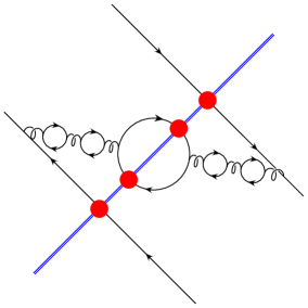
A

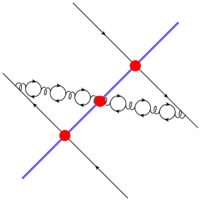
B

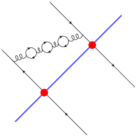
C

Figure 5: Diagrams giving the higher order $\alpha_{s}N_{f}$ corrections to the kernels of JIMWLK and BK small-$x$ evolution equations. To get the all-order $\alpha_{s}N_{f}$ contribution one has to sum an infinite series of quark bubble insertions.

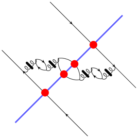
A^′

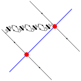
C^′

Figure 6: Diagrams giving the higher order $\alpha_{s}N_{f}$ corrections to the kernels of JIMWLK and BK small-$x$ evolution equations containing instantaneous gluon lines. Again, to get the all-order $\alpha_{s}N_{f}$ contribution one has to sum an infinite series of quark bubble insertions.

An explicit calculation using the rules of light-cone perturbation theory [41, 42] shows that inserting all-order quark bubbles on the gluon lines generates geometric series in momentum space. Before calculating the diagrams in Figs. 5 and 6 we remember that, as was discussed above, in order to find the running coupling correction, instead of the diagram in Figs. 5A and 6A^′ we should consider the “subtraction” diagrams A and A^′ shown in Fig. 7.

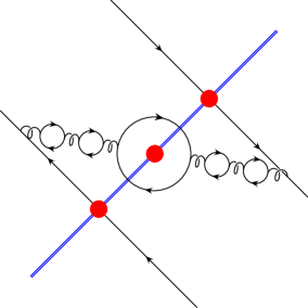
A

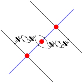
A^′

Figure 7: The “subtraction” diagrams which should be considered in place of the diagrams in Figs. 5 A and 6 A^′ for the running coupling scale calculations.

By an explicit calculation, similar to the calculation of a single bubble insertion which led to Eq. (28), one can show that the contribution of the “dressed” subtraction diagrams A and A^′ in Fig. 7 to the JIMWLK kernel reads

$$\alpha_{\mu}^{2}\,{\tilde{\cal K}}_{\begin{picture}(10.0,8.0)\put(5.0,5.0){\circle{8.0}} \put(2.9,2.5){{\scriptsize 1}} \end{picture}}({\bm{x}}_{0},{\bm{x}}_{1};{\bm{z}})\,=\,4\,\alpha_{\mu}^{2}\,\beta_{2}\,\int\frac{d^{2}q}{(2\pi)^{2}}\frac{d^{2}q^{\prime}}{(2\pi)^{2}}\ e^{-i{\bm{q}}\cdot({\bm{z}}-{\bm{x}}_{0})+i{\bm{q}}^{\prime}\cdot({\bm{z}}-{\bm{x}}_{1})}$$

$$\times\,\Bigg{\{}\frac{{\bm{q}}\cdot{\bm{q}}^{\prime}}{{\bm{q}}^{2}{\bm{q}}^{\prime 2}}\,\frac{{\bm{q}}^{2}\,\ln\frac{{\bm{q}}^{2}\,e^{-5/3}}{\mu_{\overline{{\text{MS}}}}^{2}}-{\bm{q}}^{\prime 2}\,\ln\frac{{\bm{q}}^{\prime 2}\,e^{-5/3}}{\mu_{\overline{{\text{MS}}}}^{2}}}{{\bm{q}}^{2}-{\bm{q}}^{\prime 2}}-\frac{\ln({\bm{q}}^{2}/{\bm{q}}^{\prime 2})}{{\bm{q}}^{2}-{\bm{q}}^{\prime 2}}\Bigg{\}}$$

$$\times\,\frac{1}{\left(1+\alpha_{\mu}\beta_{2}\ln\frac{{\bm{q}}^{2}\,e^{-5/3}}{\mu_{\overline{{\text{MS}}}}^{2}}\right)\,\left(1+\alpha_{\mu}\beta_{2}\ln\frac{{\bm{q}}^{\prime 2}\,e^{-5/3}}{\mu_{\overline{{\text{MS}}}}^{2}}\right)},$$ (80)

where we have also replaced all factors of $N_{f}$ by $-6\,\pi\,\beta_{2}$. Similarly, the contribution of the “dressed” diagram in Fig. 5 B is obtained by iterating the quark bubbles from Eq. (28) on both sides of the cut. The series of bubbles on each side of the cut generates a geometric series. The zeroth-order term in this series is the leading order JIMWLK kernel. The first-order term in the series is given by $K_{2}^{\text{NLO}}$ in Eq. (2.2). It is therefore more convenient to write down the sum of the LO JIMWLK kernel and the contribution of the diagram in Fig. 5 B. The result is

$$\alpha_{\mu}\,{\cal K}^{\text{LO}}({\bm{x}}_{0},{\bm{x}}_{1};{\bm{z}})+\alpha_{\mu}^{2}\,{\cal K}_{\begin{picture}(10.0,8.0)\put(5.0,5.0){\circle{8.0}} \put(2.9,2.5){{\scriptsize 2}} \end{picture}}({\bm{x}}_{0},{\bm{x}}_{1};{\bm{z}})\,=\,4\,\alpha_{\mu}\,\int\frac{d^{2}q}{(2\pi)^{2}}\frac{d^{2}q^{\prime}}{(2\pi)^{2}}\ e^{-i{\bm{q}}\cdot({\bm{z}}-{\bm{x}}_{0})+i{\bm{q}}^{\prime}\cdot({\bm{z}}-{\bm{x}}_{1})}\,\frac{{\bm{q}}\cdot{\bm{q}}^{\prime}}{{\bm{q}}^{2}{\bm{q}}^{\prime 2}}$$

$$\times\,\frac{1}{\left(1+\alpha_{\mu}\beta_{2}\ln\frac{{\bm{q}}^{2}\,e^{-5/3}}{\mu_{\overline{{\text{MS}}}}^{2}}\right)\,\left(1+\alpha_{\mu}\beta_{2}\ln\frac{{\bm{q}}^{\prime 2}\,e^{-5/3}}{\mu_{\overline{{\text{MS}}}}^{2}}\right)}.$$ (81)

The contribution to the virtual part of the JIMWLK or BK kernels is given by the diagrams in Figs. 5C and 6C^′. It can be easily extracted from Eqs. (4) and (4) using the condition (36) which holds to all orders in quark bubbles. The resulting virtual kernel would be equal to the real kernel as was explained above and shown in Eqs. (67) and (3.2). The dispersive method of [37], which was used there to calculate Figs. 5C and 6C^′, can also be used to obtain Eq. (4), and, by employing the probability conservation condition (38), to recover Eq. (4) as well.

Before proceeding to evaluate the kernels in Eqs. (4) and (4) let us first analyze their dependence on the UV cutoff $\mu_{\overline{{\text{MS}}}}$. This is instructive because the cutoff is indeed a constant and therefore $\mu_{\overline{{\text{MS}}}}$-dependence does not get modified by the Fourier transform. Hence the $\mu_{\overline{{\text{MS}}}}$-dependence of the kernel is the same in transverse coordinate and momentum spaces. Keeping only $\alpha_{\mu}$, $\beta_{2}$ and $\mu_{\overline{{\text{MS}}}}$ we thus write

$$\alpha_{\mu}^{2}\,{\tilde{\cal K}}_{\begin{picture}(10.0,8.0)\put(5.0,5.0){\circle{8.0}} \put(2.9,2.5){{\scriptsize 1}} \end{picture}}\,\propto\,\frac{-\alpha_{\mu}^{2}\,\beta_{2}\,\ln\mu_{\overline{{\text{MS}}}}^{2}}{(1-\alpha_{\mu}\beta_{2}\ln{\mu_{\overline{{\text{MS}}}}^{2}})^{2}}$$ (82)

and

$$\alpha_{\mu}\,{\cal K}^{\text{LO}}+\alpha_{\mu}^{2}\,{\cal K}_{\begin{picture}(10.0,8.0)\put(5.0,5.0){\circle{8.0}} \put(2.9,2.5){{\scriptsize 2}} \end{picture}}\,\propto\,\frac{\alpha_{\mu}}{(1-\alpha_{\mu}\beta_{2}\ln{\mu_{\overline{{\text{MS}}}}^{2}})^{2}}.$$ (83)

From Eq. (83) we immediately see that the sum of the LO kernel and the diagram in Fig. 5B does not give us a renormalizable quantity, as it can not be expressed in terms of the renormalized coupling constant. It lacks a power of $\alpha_{\mu}$ to give us a square of the physical coupling $\alpha_{s}^{2}$. Now the need of extracting the UV divergence from the graph in Fig. 5A becomes manifest. Adding the “subtraction” term (82) to (83) yields

$$\alpha_{\mu}\,{\cal K}^{\text{LO}}+\alpha_{\mu}^{2}\,{\cal K}_{\begin{picture}(10.0,8.0)\put(5.0,5.0){\circle{8.0}} \put(2.9,2.5){{\scriptsize 2}} \end{picture}}+\alpha_{\mu}^{2}\,{\tilde{\cal K}}_{\begin{picture}(10.0,8.0)\put(5.0,5.0){\circle{8.0}} \put(2.9,2.5){{\scriptsize 1}} \end{picture}}\,\propto\,\frac{\alpha_{\mu}\,(1-\alpha_{\mu}\beta_{2}\ln{\mu_{\overline{{\text{MS}}}}^{2}})}{(1-\alpha_{\mu}\beta_{2}\ln{\mu_{\overline{{\text{MS}}}}^{2}})^{2}}\,\propto\,\frac{\alpha_{s}\,\alpha_{s}}{\alpha_{s}},$$ (84)

which is indeed renormalizable as it can be expressed in terms of the physical coupling $\alpha_{s}$. (We have left a factor of $\alpha_{s}$ both in the numerator and in the denominator of Eq. (84) on purpose to underline the fact that the arguments of all three couplings, which we did not keep, may be different, which would prohibit the cancellation.)

The sum of the kernels in Eqs. (4) and (4) gives the all-order in $\alpha_{s}\,N_{f}$ (or $\alpha_{s}\,\beta_{2}$) contribution to the running-coupling part of the real JIMWLK kernel:

$$\alpha_{\mu}\, {\cal K}_{\text{rc}}({\bm{x}}_{0},{\bm{x}}_{1};{\bm{z}})\,\equiv\,\alpha_{\mu}\,{\cal K}^{\text{LO}}({\bm{x}}_{0},{\bm{x}}_{1};{\bm{z}})+\alpha_{\mu}^{2}\,{\cal K}_{\bigcirc 2}({\bm{x}}_{0},{\bm{x}}_{1};{\bm{z}})+\alpha_{\mu}^{2}\,{\tilde{\cal K}}_{\bigcirc 1}({\bm{x}}_{0},{\bm{x}}_{1};{\bm{z}})\,=$$

$$=\,4\,\int\frac{d^{2}q}{(2\pi)^{2}}\frac{d^{2}q^{\prime}}{(2\pi)^{2}}\ e^{-i{\bm{q}}\cdot({\bm{z}}-{\bm{x}}_{0})+i{\bm{q}}^{\prime}\cdot({\bm{z}}-{\bm{x}}_{1})}\,\frac{{\bm{q}}\cdot{\bm{q}}^{\prime}}{{\bm{q}}^{2}\,{\bm{q}}^{\prime 2}}\,\frac{\alpha_{\mu}\,\left(1+\alpha_{\mu}\beta_{2}\,\ln\frac{Q^{2}\,e^{-5/3}}{\mu_{\overline{{\text{MS}}}}^{2}}\right)}{\left(1+\alpha_{\mu}\beta_{2}\ln\frac{{\bm{q}}^{2}\,e^{-5/3}}{\mu_{\overline{{\text{MS}}}}^{2}}\right)\,\left(1+\alpha_{\mu}\beta_{2}\ln\frac{{\bm{q}}^{\prime 2}\,e^{-5/3}}{\mu_{\overline{{\text{MS}}}}^{2}}\right)}$$ (85)

where we have defined a momentum scale $Q$ by

$$\ln\frac{Q^{2}\,e^{-5/3}}{\mu_{\overline{{\text{MS}}}}^{2}}\,\equiv\,\frac{{\bm{q}}^{2}\,\ln\frac{{\bm{q}}^{2}\,e^{-5/3}}{\mu_{\overline{{\text{MS}}}}^{2}}-{\bm{q}}^{\prime 2}\,\ln\frac{{\bm{q}}^{\prime 2}\,e^{-5/3}}{\mu_{\overline{{\text{MS}}}}^{2}}}{{\bm{q}}^{2}-{\bm{q}}^{\prime 2}}-\frac{{\bm{q}}^{2}\,{\bm{q}}^{\prime 2}}{{\bm{q}}\cdot{\bm{q}}^{\prime}}\,\frac{\ln({\bm{q}}^{2}/{\bm{q}}^{\prime 2})}{{\bm{q}}^{2}-{\bm{q}}^{\prime 2}}.$$ (86)

(Indeed $Q^{2}$ is independent of $\mu_{\overline{{\text{MS}}}}$ as can be easily seen from Eq. (86).) As the one-loop running coupling constant is defined in the $\overline{{\text{MS}}}$ scheme by

$$\alpha_{s}(Q^{2})\,=\,\frac{\alpha_{\mu}}{1+\alpha_{\mu}\beta_{2}\,\ln\frac{Q^{2}}{\mu_{\overline{{\text{MS}}}}^{2}}}$$ (87)

Eq. (4) can be rewritten as

$$\alpha_{\mu}\, {\cal K}_{\text{rc}}({\bm{x}}_{0},{\bm{x}}_{1};{\bm{z}})\,\equiv\,\alpha_{\mu}\,{\cal K}^{\text{LO}}({\bm{x}}_{0},{\bm{x}}_{1};{\bm{z}})+\alpha_{\mu}^{2}\,{\cal K}_{\bigcirc 2}({\bm{x}}_{0},{\bm{x}}_{1};{\bm{z}})+\alpha_{\mu}^{2}\,{\tilde{\cal K}}_{\bigcirc 1}({\bm{x}}_{0},{\bm{x}}_{1};{\bm{z}})\,=$$

$$=\,4\,\int\frac{d^{2}q}{(2\pi)^{2}}\frac{d^{2}q^{\prime}}{(2\pi)^{2}}\ e^{-i{\bm{q}}\cdot({\bm{z}}-{\bm{x}}_{0})+i{\bm{q}}^{\prime}\cdot({\bm{z}}-{\bm{x}}_{1})}\,\frac{{\bm{q}}\cdot{\bm{q}}^{\prime}}{{\bm{q}}^{2}\,{\bm{q}}^{\prime 2}}\,\frac{\alpha_{s}\left({\bm{q}}^{2}\,e^{-5/3}\right)\,\alpha_{s}\left({\bm{q}}^{\prime 2}\,e^{-5/3}\right)}{\alpha_{s}\left(Q^{2}\,e^{-5/3}\right)}\ .$$ (88)

Eq. (4) is the first of the two main results of our paper. It gives the JIMWLK kernel with the running coupling corrections included in transverse momentum space. Remarkably, the corrections come in as a “triumvirate” of the couplings, instead of a single coupling constant with some momentum scale! Despite the surprising form this result is in full agreement with the expressions found in[37]. To facilitate comparison, we give a detailed translation in appendix. C

This provides for an interesting mechanism to reduce the above result to a simpler underlying structure expected for the purely virtual contributions of diagrams Fig. 5 C and 6 C’: There the $z$ integral may be performed and, in the absence of interaction with the target, this sets ${\bm{q}}^{\prime}={\bm{q}}$. Then the sum of the integrands of transverse and longitudinal contributions reduces to

$$\alpha_{\mu}\,\frac{\frac{1}{\bm{q}^{2}}\left\{1+\alpha_{\mu}\beta_{2}\,\left[1+\ln\left(\frac{{\bm{q}}^{2}\,e^{-\frac{5}{3}}}{\mu^{2}_{\overline{{\text{MS}}}}}\right)\right]\right\}-\frac{1}{\bm{q}^{2}}\alpha_{\mu}\beta_{2}}{\left(1+\beta_{2}\alpha_{\mu}\,\ln\left(\frac{{\bm{q}}^{2}\,e^{-\frac{5}{3}}}{\mu^{2}_{\overline{{\text{MS}}}}}\right)\right)^{2}}=\frac{1}{\bm{q}^{2}}\ \alpha_{s}\left({\bm{q}}^{2}\,e^{-\frac{5}{3}}\right)$$ (89)

which clearly corresponds to the exchange of a dressed noninteracting gluon. This is the counterpart of a cancellation that appears in [37] under the same premise. Note that due to the virtual nature of the diagrams in Figs. 5 C and 6 C’ the running coupling corrections can enter only with the sole available transverse momentum scale ${\bm{q}}^{2}$ in its argument, as shown in Eq. (89). Therefore, while different subtraction procedures may yield different expressions for the scale $Q$, as compared to Eq. (86), all of these alternatives must lead to expressions for $Q^{2}$ that approach ${\bm{q}}^{2}$ in the limit when ${\bm{q}}^{\prime}={\bm{q}}$. This would reduce the “triumvirate” of couplings from Eq. (4) to the single coupling shown in Eq. (89), as expected for virtual diagrams here.

The most intriguing property, however, is that the “triumvirate” structure of (4) solves the puzzle of how to successfully perform a BLM scale setting: In [37] it was observed that an attempt to perform a BLM scale setting in a perturbative formulation with a single Borel parameter (corresponding to an approximation in terms of a single geometric series in our present language) would not lead to a successful resummation of the dominant contribution. From the present perspective this would correspond to the attempt to use the joint leading order expansion of all three couplings in (4) to determine a single scale (instead of the three separate ones of (4)) that would give a good approximation to the triumvirate in terms of a single geometric series. Any such attempt would necessarily entail an artificial all orders iteration of the “numerator logarithms” encoded in the “denominator coupling” $\alpha_{s}(Q^{2}e^{-\frac{5}{3}})$ that is clearly absent in the underlying expression. This is the source of the spurious and divergent higher inverse powers of ${\bm{q}}\cdot{\bm{q}}^{\prime}$ or $(\bm{x}_{0}-\bm{z})\cdot(\bm{x}_{1}-\bm{z})$ encountered in a naive attempt of deriving a BLM approximation in [37]. The “triumvirate” structure will allow for a successful and transparent BLM approximation of the full coordinate result given in [37].

Eq. (4) allows one to find the corresponding BK evolution kernel with the running coupling corrections included by using

$$K_{\text{rc}}({\bm{x}}_{0},{\bm{x}}_{1};{\bm{z}})\,=\,C_{F}\,\sum_{m,n=0}^{1}\,(-1)^{m+n}\,{\cal K}_{\text{rc}} ({\bm{x}}_{m},{\bm{x}}_{n};{\bm{z}}).$$ (90)

To determine the scales of the three physical couplings in Eq. (4) in transverse coordinate space we have to evaluate the integrations in the kernels from Eqs. (4) and (4). In transverse momentum space each chain of bubbles generates a geometric series, as shown in Eq. (4). However, a Fourier-transform of these series is dangerous for several reasons. First and foremost the integrals over ${\bm{q}}$ and ${\bm{q}}^{\prime}$ in Eqs. (4) and (4) include contributions from the Landau poles leading to power corrections which are not under perturbative control. The uncertainties due to power corrections are estimated in [37] using renormalon techniques [50, 51]. Our strategy here is to ignore these contributions concentrating on setting the scale of the running coupling in transverse coordinate space. Even then our goal is difficult, since, even though leading powers of $\ln\mu_{\overline{{\text{MS}}}}^{2}$ terms generate a geometric series in transverse coordinate space just like in the momentum space, it is not clear whether the transverse coordinate scale under the logarithm stays the same in all the terms in the series. In that sense, setting the running coupling scale in transverse coordinate space will only be an approximation of the more exact Eq. (4) in the sense of a BLM scale setting.

To study running coupling corrections in transverse coordinate space we begin by evaluating the Fourier transforms in Eq. (4). Similar to Appendix A we perform the angular integrals first to write

$$\alpha_{\mu}\,{\cal K}^{\text{LO}}({\bm{x}}_{0},{\bm{x}}_{1};{\bm{z}})+\alpha_{\mu}^{2}\,{\cal K}_{\begin{picture}(10.0,8.0)\put(5.0,5.0){\circle{8.0}} \put(2.9,2.5){{\scriptsize 2}} \end{picture}}({\bm{x}}_{0},{\bm{x}}_{1};{\bm{z}})\,=\,\frac{\alpha_{\mu}}{\pi^{2}}\,\frac{{\bm{z}}-{\bm{x}}_{0}}{|{\bm{z}}-{\bm{x}}_{0}|}\cdot\frac{{\bm{z}}-{\bm{x}}_{1}}{|{\bm{z}}-{\bm{x}}_{1}|}$$

$$\times\,\int\limits_{0}^{\infty}dq\,dq^{\prime}\,J_{1}(q\,|{\bm{z}}-{\bm{x}}_{0}|)\,J_{1}(q^{\prime}\,|{\bm{z}}-{\bm{x}}_{1}|)\,\frac{1}{\left(1+\alpha_{\mu}\beta_{2}\ln\frac{q^{2}\,e^{-5/3}}{\mu_{\overline{{\text{MS}}}}^{2}}\right)\,\left(1+\alpha_{\mu}\beta_{2}\ln\frac{q^{\prime 2}\,e^{-5/3}}{\mu_{\overline{{\text{MS}}}}^{2}}\right)}$$ (91)

with $q=|{\bm{q}}|$ and $q^{\prime}=|{\bm{q}}^{\prime}|$. Since our goal is to find the scale of the strong coupling constant ignoring the power corrections we can expand the denominators of Eq. (4) into geometric series obtaining

$$\alpha_{\mu}\,{\cal K}^{\text{LO}}({\bm{x}}_{0},{\bm{x}}_{1};{\bm{z}})+\alpha_{\mu}^{2}\,{\cal K}_{\begin{picture}(10.0,8.0)\put(5.0,5.0){\circle{8.0}} \put(2.9,2.5){{\scriptsize 2}} \end{picture}}({\bm{x}}_{0},{\bm{x}}_{1};{\bm{z}})\,=\,\frac{\alpha_{\mu}}{\pi^{2}}\,\frac{{\bm{z}}-{\bm{x}}_{0}}{|{\bm{z}}-{\bm{x}}_{0}|}\cdot\frac{{\bm{z}}-{\bm{x}}_{1}}{|{\bm{z}}-{\bm{x}}_{1}|}\,\sum\limits_{n,m=0}^{\infty}\,(-\alpha_{\mu}\beta_{2})^{n+m}$$

$$\times\,\int\limits_{0}^{\infty}dq\,dq^{\prime}\,J_{1}(q\,|{\bm{z}}-{\bm{x}}_{0}|)\,J_{1}(q^{\prime}\,|{\bm{z}}-{\bm{x}}_{1}|)\ln^{n}\frac{q^{2}\,e^{-5/3}}{\mu_{\overline{{\text{MS}}}}^{2}}\,\ln^{m}\frac{q^{\prime 2}\,e^{-5/3}}{\mu_{\overline{{\text{MS}}}}^{2}}.$$ (92)

Rewriting the powers of the logarithms in Eq. (4) in terms of derivatives yields

$$\alpha_{\mu}\,{\cal K}^{\text{LO}}({\bm{x}}_{0},{\bm{x}}_{1};{\bm{z}})+\alpha_{\mu}^{2}\,{\cal K}_{\begin{picture}(10.0,8.0)\put(5.0,5.0){\circle{8.0}} \put(2.9,2.5){{\scriptsize 2}} \end{picture}}({\bm{x}}_{0},{\bm{x}}_{1};{\bm{z}})\,=\,\frac{\alpha_{\mu}}{\pi^{2}}\,\frac{{\bm{z}}-{\bm{x}}_{0}}{|{\bm{z}}-{\bm{x}}_{0}|}\cdot\frac{{\bm{z}}-{\bm{x}}_{1}}{|{\bm{z}}-{\bm{x}}_{1}|}\,\sum\limits_{n,m=0}^{\infty}\,(-\alpha_{\mu}\beta_{2})^{n+m}$$

$$\times\,\frac{d^{n}}{d\lambda^{n}}\,\frac{d^{m}}{d\lambda^{\prime m}}\,\int\limits_{0}^{\infty}dq\,dq^{\prime}\,J_{1}(q\,|{\bm{z}}-{\bm{x}}_{0}|)\,J_{1}(q^{\prime}\,|{\bm{z}}-{\bm{x}}_{1}|)\left(\frac{q^{2}\,e^{-5/3}}{\mu_{\overline{{\text{MS}}}}^{2}}\right)^{\lambda}\,\left(\frac{q^{\prime 2}\,e^{-5/3}}{\mu_{\overline{{\text{MS}}}}^{2}}\right)^{\lambda^{\prime}}\Bigg{|}_{\lambda,\lambda^{\prime}=0}.$$ (93)

Performing the $q$- and $q^{\prime}$-integrals gives

$$\alpha_{\mu}\,{\cal K}^{\text{LO}}({\bm{x}}_{0},{\bm{x}}_{1};{\bm{z}})+\alpha_{\mu}^{2}\,{\cal K}_{\begin{picture}(10.0,8.0)\put(5.0,5.0){\circle{8.0}} \put(2.9,2.5){{\scriptsize 2}} \end{picture}}({\bm{x}}_{0},{\bm{x}}_{1};{\bm{z}})\,= \,\alpha_{\mu}\,{\cal K}^{\text{LO}}({\bm{x}}_{0},{\bm{x}}_{1};{\bm{z}})\,\sum\limits_{n,m=0}^{\infty}\,(-\alpha_{\mu}\beta_{2})^{n+m}$$

$$\times\left\{\frac{d^{n}}{d\lambda^{n}}\left[\left(\frac{4\,e^{-5/3}}{|{\bm{z}}-{\bm{x}}_{0}|^{2}\,\mu_{\overline{{\text{MS}}}}^{2}}\right)^{\lambda}\frac{\Gamma(1+\lambda)}{\Gamma(1-\lambda)}\right]\right\}\Bigg{|}_{\lambda=0} \left\{\frac{d^{m}}{d\lambda^{m}}\left[\left(\frac{4\,e^{-5/3}}{|{\bm{z}}-{\bm{x}}_{1}|^{2}\,\mu_{\overline{{\text{MS}}}}^{2}}\right)^{\lambda^{\prime}}\frac{\Gamma(1+\lambda^{\prime})}{\Gamma(1-\lambda^{\prime})}\right]\right\}\Bigg{|}_{\lambda^{\prime}=0}.$$ (94)

Differentiating with respect to $\lambda$ and $\lambda^{\prime}$ we write out the first few terms in the resulting series

$$\alpha_{\mu}\,{\cal K}^{\text{LO}}({\bm{x}}_{0},{\bm{x}}_{1};{\bm{z}})+\alpha_{\mu}^{2}\,{\cal K}_{\begin{picture}(10.0,8.0)\put(5.0,5.0){\circle{8.0}} \put(2.9,2.5){{\scriptsize 2}} \end{picture}}({\bm{x}}_{0},{\bm{x}}_{1};{\bm{z}})\,= \,\alpha_{\mu}\,{\cal K}^{\text{LO}}({\bm{x}}_{0},{\bm{x}}_{1};{\bm{z}})$$

$$\times\,\Bigg{\{}1-\alpha_{\mu}\beta_{2}\,\ln\left(\frac{4\,e^{-5/3-2\gamma}}{|{\bm{z}}-{\bm{x}}_{0}|^{2}\,\mu_{\overline{{\text{MS}}}}^{2}}\right)+ (\alpha_{\mu}\beta_{2})^{2}\,\ln^{2}\left(\frac{4\,e^{-5/3-2\gamma}}{|{\bm{z}}-{\bm{x}}_{0}|^{2}\,\mu_{\overline{{\text{MS}}}}^{2}}\right)$$

$$-(\alpha_{\mu}\beta_{2})^{3}\, \left[\ln^{3}\left(\frac{4\,e^{-5/3-2\gamma}}{|{\bm{z}}-{\bm{x}}_{0}|^{2}\,\mu_{\overline{{\text{MS}}}}^{2}}\right)-4\,\zeta(3)\right]+\ldots\Bigg{\}}\,$$

$$\times\,\Bigg{\{}1-\alpha_{\mu}\beta_{2}\,\ln\left(\frac{4\,e^{-5/3-2\gamma}}{|{\bm{z}}-{\bm{x}}_{1}|^{2}\,\mu_{\overline{{\text{MS}}}}^{2}}\right)+ (\alpha_{\mu}\beta_{2})^{2}\,\ln^{2}\left(\frac{4\,e^{-5/3-2\gamma}}{|{\bm{z}}-{\bm{x}}_{1}|^{2}\,\mu_{\overline{{\text{MS}}}}^{2}}\right)$$

$$-(\alpha_{\mu}\beta_{2})^{3}\, \left[\ln^{3}\left(\frac{4\,e^{-5/3-2\gamma}}{|{\bm{z}}-{\bm{x}}_{1}|^{2}\,\mu_{\overline{{\text{MS}}}}^{2}}\right)-4\,\zeta(3)\right]+\ldots\Bigg{\}}.$$ (95)

One can see that the geometric series structure appears to hold up to the cubic terms in either one of the logarithms. In the sense of a BLM-type approach [43] we approximate the expressions in each of the curly brackets by a geometric series, obtaining

$$\alpha_{\mu}\,{\cal K}^{\text{LO}}({\bm{x}}_{0},{\bm{x}}_{1};{\bm{z}})+ \alpha_{\mu}^{2}\,{\cal K}_{\begin{picture}(10.0,8.0)\put(5.0,5.0){\circle{8.0}} \put(2.9,2.5){{\scriptsize 2}} \end{picture}}({\bm{x}}_{0},{\bm{x}}_{1};{\bm{z}})\,\approx\,{\cal K}^{\text{LO}}({\bm{x}}_{0},{\bm{x}}_{1};{\bm{z}})$$

$$\times \,\frac{\alpha_{\mu}}{\left[1+\alpha_{\mu}\beta_{2}\,\ln\left(\frac{4\,e^{-5/3-2\gamma}}{|{\bm{z}}-{\bm{x}}_{0}|^{2}\,\mu_{\overline{{\text{MS}}}}^{2}}\right)\right]\,\left[1+\alpha_{\mu}\beta_{2}\,\ln\left(\frac{4\,e^{-5/3-2\gamma}}{|{\bm{z}}-{\bm{x}}_{1}|^{2}\,\mu_{\overline{{\text{MS}}}}^{2}}\right)\right]}.$$ (96)

Evaluation of the Fourier transforms in Eq. (4) is performed along similar lines in Appendix B. The result reads

$$\alpha_{\mu}^{2}\,{\tilde{\cal K}}_{\begin{picture}(10.0,8.0)\put(5.0,5.0){\circle{8.0}} \put(2.9,2.5){{\scriptsize 1}} \end{picture}}({\bm{x}}_{0},{\bm{x}}_{1};{\bm{z}})\,\approx\,{\cal K}^{\text{LO}}({\bm{x}}_{0},{\bm{x}}_{1};{\bm{z}})\,\alpha_{\mu}\beta_{2}\,\ln\left(\frac{4\,e^{-\frac{5}{3}-2\gamma}}{R^{2}({\bm{x}}_{0},{\bm{x}}_{1};{\bm{z}})\,\mu_{\overline{{\text{MS}}}}^{2}}\right)$$

$$\times\,\frac{\alpha_{\mu}}{\left[1+\alpha_{\mu}\beta_{2}\,\ln\left(\frac{4\,e^{-5/3-2\gamma}}{|{\bm{z}}-{\bm{x}}_{0}|^{2}\,\mu_{\overline{{\text{MS}}}}^{2}}\right)\right]\,\left[1+\alpha_{\mu}\beta_{2}\,\ln\left(\frac{4\,e^{-5/3-2\gamma}}{|{\bm{z}}-{\bm{x}}_{1}|^{2}\,\mu_{\overline{{\text{MS}}}}^{2}}\right)\right]},$$ (97)

with the scale $R$ given by Eq. (45).

Finally, adding Eqs. (4) and (4) yields

$$\alpha_{\mu}\, {\cal K}_{\text{rc}}({\bm{x}}_{0},{\bm{x}}_{1};{\bm{z}})\,\approx\,{\cal K}^{\text{LO}}({\bm{x}}_{0},{\bm{x}}_{1};{\bm{z}})\,\frac{\alpha_{s}\left(\frac{4\,e^{-5/3-2\gamma}}{|{\bm{z}}-{\bm{x}}_{0}|^{2}}\right)\ \alpha_{s}\left(\frac{4\,e^{-5/3-2\gamma}}{|{\bm{z}}-{\bm{x}}_{1}|^{2}}\right)}{\alpha_{s}\left(\frac{4\,e^{-5/3-2\gamma}}{R^{2}({\bm{x}}_{0},{\bm{x}}_{1};{\bm{z}})}\right)}$$ (98)

with the scale $R({\bm{x}}_{0},{\bm{x}}_{1};{\bm{z}})$ given by Eq. (45) and the couplings calculated in the $\overline{{\text{MS}}}$ scheme. Eq. (98) is the second of the two main results of our paper. It gives the JIMWLK kernel with the running coupling constant. It is very interesting that the running coupling corrections come in not through a scale of a single running coupling $\alpha_{s}$ as one would naively expect, but in the form of a “triumvirate” of the running couplings shown in Eq. (98)! Eq. (98) can be used to construct BK kernel with the running coupling constant by employing Eq. (90).

5 Conclusions

To conclude let us state the main results of this work once again. By tracking the powers of $\alpha_{s}\,N_{f}$ we have included running coupling corrections into the JIMWLK and BK evolution equations. Our all orders result agrees with the expressions derived with the dispersive method in [37], but renders the result in terms of a “triumvirate” of couplings already in the momentum space expressions (4). This allows us to give a concise, accurate BLM approximation of the perturbative sum in coordinate space in terms of a corresponding coordinate space “triumvirate” shown in Eq. (98). Our procedure includes one uncertainty, related to choosing the “subtraction point”, as was discussed in Sect. 3. This ambiguity is akin to scheme-dependence of the running coupling constant and we believe that the final result does not depend on the choice of the “subtraction point” in a very crucial way. We picked the subtraction point to be at the transverse coordinate of the virtual gluon in Fig. 1A.

Our result for the JIMWLK Hamiltonian with the running coupling constant is

$${\cal H}^{\text{rc}}=\frac{1}{2}\,\frac{\alpha_{s}\left(\frac{4\,e^{-5/3-2\gamma}}{|{\bm{z}}-{\bm{x}}|^{2}}\right)\,\alpha_{s}\left(\frac{4\,e^{-5/3-2\gamma}}{|{\bm{z}}-{\bm{y}}|^{2}}\right)}{\alpha_{s}\left(\frac{4\,e^{-5/3-2\gamma}}{R^{2}({\bm{x}},{\bm{y}};{\bm{z}})}\right)}\,{\cal K}^{\text{LO}}_{{\bm{x}},{\bm{y}};{\bm{z}}}\left[U_{\bm{z}}^{ab}(i\bar{\nabla}^{a}_{\bm{x}}i\nabla^{b}_{\bm{y}}+i\nabla^{a}_{\bm{x}}i\bar{\nabla}^{b}_{\bm{y}})+(i\nabla^{a}_{\bm{x}}i\nabla^{a}_{\bm{y}}+i\bar{\nabla}^{a}_{\bm{x}}i\bar{\nabla}^{a}_{\bm{y}})\right]$$ (99)

with integrations over $\bm{x}$, $\bm{y}$ and $\bm{z}$ implied. All the running couplings should be calculated in the $\overline{{\text{MS}}}$ scheme.

To obtain the BK evolution equation with the running coupling constant one needs to sum the kernel in Eq. (98) over all possible connections of the gluon to the quark and the anti-quark lines, as formally shown in Eq. (90). (Alternatively to derive the BK equation one can apply the JIMWLK Hamiltonian from Eq. (99) to a correlator of two Wilson lines and take the large-$N_{c}$ limit.) A straightforward calculation shows that

$$\lim_{{\bm{x}}_{1}\rightarrow{\bm{x}}_{0}}R^{2}({\bm{x}}_{0},{\bm{x}}_{1};{\bm{z}})\,=\,|{\bm{z}}-{\bm{x}}_{0}|^{2}\hskip 28.45274pt\text{and}\hskip 28.45274pt\lim_{{\bm{x}}_{0}\rightarrow{\bm{x}}_{1}}R^{2}({\bm{x}}_{0},{\bm{x}}_{1};{\bm{z}})\,=\,|{\bm{z}}-{\bm{x}}_{1}|^{2},$$ (100)

such that the BK evolution equation with the running coupling corrections is

$$\frac{\partial N({\bm{x}}_{0},{\bm{x}}_{1},Y)}{\partial Y}\,=\,\frac{C_{F}}{\pi^{2}}\,\int d^{2}x_{2}$$

$$\times\,\left[\alpha_{s}\left(\frac{4\,e^{-5/3-2\gamma}}{x_{20}^{2}}\right)\,\frac{1}{x_{20}^{2}}-2\,\frac{\alpha_{s}\left(\frac{4\,e^{-5/3-2\gamma}}{x_{20}^{2}}\right)\ \alpha_{s}\left(\frac{4\,e^{-5/3-2\gamma}}{x_{21}^{2}}\right)}{\alpha_{s}\left(\frac{4\,e^{-5/3-2\gamma}}{R^{2}({\bm{x}}_{0},{\bm{x}}_{1};\,{\bm{x}}_{2})}\right)}\,\frac{{\bm{x}}_{20}\cdot{\bm{x}}_{21}}{x_{20}^{2}\,x_{21}^{2}}+\alpha_{s}\left(\frac{4\,e^{-5/3-2\gamma}}{x_{21}^{2}}\right)\,\frac{1}{x_{21}^{2}}\right]$$

$$\times\,\left[N({\bm{x}}_{0},{\bm{x}}_{2},Y)+N({\bm{x}}_{2},{\bm{x}}_{1},Y)-N({\bm{x}}_{0},{\bm{x}}_{1},Y)-N({\bm{x}}_{0},{\bm{x}}_{2},Y)\,N({\bm{x}}_{2},{\bm{x}}_{1},Y)\right],$$ (101)

where $R^{2}$ is given by Eq. (45).

It is interesting to explore the limits of Eq. (5). We will refer to the original dipole $01$ as the “parent” dipole, while the dipoles $20$ and $21$ generated in one step of the evolution will be called “daughter” dipoles. First of all, when both produced dipoles are comparable and much larger than the “parent” dipole, $x_{20}\sim x_{21}\gg x_{01}$, the argument of the coupling constant in all three terms in Eq. (5) would be given by the “daughter” dipole sizes $x_{20}\sim x_{21}$. However, such large dipole sizes should be cut off by the inverse saturation scale $1/Q_{s}$, which implies that the scale for the coupling constant in the IR region of phase space would be given by $Q_{s}$ keeping the coupling small and the physics perturbative. In the other interesting limit when one of the “daughter” dipoles is much smaller than the other one, $x_{20}\ll x_{21}\sim x_{01}$, a simple calculation shows that $R^{2}({\bm{x}}_{0},{\bm{x}}_{1};\,{\bm{x}}_{2})\approx x_{20}^{2}$ and the BK kernel in Eq. (5) becomes

$$\alpha_{s}\left(\frac{4\,e^{-5/3-2\gamma}}{x_{20}^{2}}\right)\,\frac{1}{x_{20}^{2}}-2\,\alpha_{s}\left(\frac{4\,e^{-5/3-2\gamma}}{x_{21}^{2}}\right)\,\frac{{\bm{x}}_{20}\cdot{\bm{x}}_{21}}{x_{20}^{2}\,x_{21}^{2}}+\alpha_{s}\left(\frac{4\,e^{-5/3-2\gamma}}{x_{21}^{2}}\right)\,\frac{1}{x_{21}^{2}}.$$ (102)

Two out of three terms in the kernel have the scale of the coupling given by the larger dipole size, naively making the evolution “less perturbative”. However, in the $x_{20}\ll x_{21}$ limit it is the first term which dominates Eq. (102): that term has the running coupling scale given by the size of the smaller dipole, making the physics perturbative!

Appendix A Evaluating the Fourier transforms in Eq. (2.3)

Here we first calculate the following integral coming from the first (transverse) term in Eq. (2.3)

$$I_{T}({\bm{z}},{\bm{z}}^{\prime})\,=\,\int\frac{d^{2}q}{(2\pi)^{2}}\frac{d^{2}q^{\prime}}{(2\pi)^{2}}\ e^{-i{\bm{q}}\cdot{\bm{z}}+i{\bm{q}}^{\prime}\cdot{\bm{z}}^{\prime}}\,\frac{{\bm{q}}\cdot{\bm{q}}^{\prime}}{{\bm{q}}^{2}{\bm{q}}^{\prime 2}}\,\frac{{\bm{q}}^{2}\,\left(\ln\frac{{\bm{q}}^{2}}{\mu_{\overline{{\text{MS}}}}^{2}}-\frac{5}{3}\right)-{\bm{q}}^{\prime 2}\,\left(\ln\frac{{\bm{q}}^{\prime 2}}{\mu_{\overline{{\text{MS}}}}^{2}}-\frac{5}{3}\right)}{{\bm{q}}^{2}-{\bm{q}}^{\prime 2}},$$ (A1)

where ${\bm{z}}$ and ${\bm{z}}^{\prime}$ are some transverse coordinate vectors. Replacing ${\bm{q}}\rightarrow i\,{\bm{\partial}}_{z}$ and ${\bm{q}}^{\prime}\rightarrow-i\,{\bm{\partial}}_{z^{\prime}}$ in the numerator of the first ratio in the integrand we can integrate over the angles of ${\bm{q}}$ and ${\bm{q}}^{\prime}$ obtaining

$$I_{T}({\bm{z}},{\bm{z}}^{\prime})\,=\,\frac{1}{(2\pi)^{2}}\,{\bm{\partial}}_{z}\cdot{\bm{\partial}}_{z^{\prime}}\,\int\limits_{0}^{\infty}\frac{dq}{q}\,\frac{dq^{\prime}}{q^{\prime}}\,J_{0}(q\,z)\,J_{0}(q^{\prime}\,z^{\prime})\,\frac{{\bm{q}}^{2}\,\left(\ln\frac{{\bm{q}}^{2}}{\mu_{\overline{{\text{MS}}}}^{2}}-\frac{5}{3}\right)-{\bm{q}}^{\prime 2}\,\left(\ln\frac{{\bm{q}}^{\prime 2}}{\mu_{\overline{{\text{MS}}}}^{2}}-\frac{5}{3}\right)}{{\bm{q}}^{2}-{\bm{q}}^{\prime 2}}$$ (A2)

with $q=|{\bm{q}}|$, $q^{\prime}=|{\bm{q}}^{\prime}|$, $z=|{\bm{z}}|$ and $z^{\prime}=|{\bm{z}}^{\prime}|$. Bringing the transverse gradients back into the integrand yields

$$I_{T}({\bm{z}},{\bm{z}}^{\prime})\,=\,\frac{1}{(2\pi)^{2}}\,\frac{{\bm{z}}\cdot{\bm{z}}^{\prime}}{z\,z^{\prime}}\,\int\limits_{0}^{\infty}dq\,dq^{\prime}\,J_{1}(q\,z)\,J_{1}(q^{\prime}\,z^{\prime})\,\frac{{\bm{q}}^{2}\,\ln\frac{{\bm{q}}^{2}\,e^{-5/3}}{\mu_{\overline{{\text{MS}}}}^{2}}-{\bm{q}}^{\prime 2}\,\ln\frac{{\bm{q}}^{\prime 2}\,e^{-5/3}}{\mu_{\overline{{\text{MS}}}}^{2}}}{{\bm{q}}^{2}-{\bm{q}}^{\prime 2}}.$$ (A3)

To perform $q$ and $q^{\prime}$ integrations we first rewrite the fraction in the integrand of (A3) as

$$\frac{{\bm{q}}^{2}\,\ln\frac{{\bm{q}}^{2}\,e^{-5/3}}{\mu_{\overline{{\text{MS}}}}^{2}}-{\bm{q}}^{\prime 2}\,\ln\frac{{\bm{q}}^{\prime 2}\,e^{-5/3}}{\mu_{\overline{{\text{MS}}}}^{2}}}{{\bm{q}}^{2}-{\bm{q}}^{\prime 2}}\,=\,\ln\frac{{\bm{q}}^{2}\,e^{-5/3}}{\mu_{\overline{{\text{MS}}}}^{2}}+{\bm{q}}^{\prime 2}\,\frac{\ln\frac{{\bm{q}}^{2}}{{\bm{q}}^{\prime 2}}}{{\bm{q}}^{2}-{\bm{q}}^{\prime 2}}$$ (A4)

and then use the following integral identity

$$\int\limits_{0}^{1}d\beta\,\frac{1}{{\bm{q}}^{2}(1-\beta)+{\bm{q}}^{\prime 2}\beta}\,=\,\frac{\ln\frac{{\bm{q}}^{2}}{{\bm{q}}^{\prime 2}}}{{\bm{q}}^{2}-{\bm{q}}^{\prime 2}}$$ (A5)

to replace the last term in Eq. (A4). Eq. (A3) becomes

$$I_{T}({\bm{z}},{\bm{z}}^{\prime})\,=\,\frac{1}{(2\pi)^{2}}\,\frac{{\bm{z}}\cdot{\bm{z}}^{\prime}}{z\,z^{\prime}}\,\int\limits_{0}^{\infty}dq\,dq^{\prime}\,J_{1}(q\,z)\,J_{1}(q^{\prime}\,z^{\prime})\,\left\{\ln\frac{{\bm{q}}^{2}\,e^{-5/3}}{\mu_{\overline{{\text{MS}}}}^{2}}+{\bm{q}}^{\prime 2}\,\int\limits_{0}^{1}d\beta\,\frac{1}{{\bm{q}}^{2}(1-\beta)+{\bm{q}}^{\prime 2}\beta}\right\}.$$ (A6)

Now the $q$ and $q^{\prime}$ integrations can be performed using standard formulas for the integrals of Bessel functions yielding

$$I_{T}({\bm{z}},{\bm{z}}^{\prime})\,=\,\frac{1}{(2\pi)^{2}}\,\frac{{\bm{z}}\cdot{\bm{z}}^{\prime}}{{\bm{z}}^{2}\,{\bm{z}}^{\prime 2}}\,\left\{\ln\frac{4\,e^{-\frac{5}{3}-2\gamma}}{{\bm{z}}^{2}\,\mu_{\overline{{\text{MS}}}}^{2}}+{\bm{z}}^{2}\,\int\limits_{0}^{1}d\beta\,\frac{1}{{\bm{z}}^{2}(1-\beta)+{\bm{z}}^{\prime 2}\beta}\right\}.$$ (A7)

Finally the $\beta$-integral in Eq. (A7) can be done using Eq. (A5) giving

$$I_{T}({\bm{z}},{\bm{z}}^{\prime})\,=\,\frac{1}{(2\pi)^{2}}\,\frac{{\bm{z}}\cdot{\bm{z}}^{\prime}}{{\bm{z}}^{2}\,{\bm{z}}^{\prime 2}}\,\frac{{\bm{z}}^{2}\,\ln\frac{4\,e^{-\frac{5}{3}-2\gamma}}{{\bm{z}}^{\prime 2}\,\mu_{\overline{{\text{MS}}}}^{2}}-{\bm{z}}^{\prime 2}\,\ln\frac{4\,e^{-\frac{5}{3}-2\gamma}}{{\bm{z}}^{2}\,\mu_{\overline{{\text{MS}}}}^{2}}}{{\bm{z}}^{2}-{\bm{z}}^{\prime 2}}.$$ (A8)

Now let us use the same technique to perform Fourier transforms in the second (longitudinal) term in Eq. (2.3). We want to evaluate

$$I_{L}({\bm{z}},{\bm{z}}^{\prime})\,=\,\int\frac{d^{2}q}{(2\pi)^{2}}\frac{d^{2}q^{\prime}}{(2\pi)^{2}}\ e^{-i{\bm{q}}\cdot{\bm{z}}+i{\bm{q}}^{\prime}\cdot{\bm{z}}^{\prime}}\,\frac{\ln({\bm{q}}^{2}/{\bm{q}}^{\prime 2})}{{\bm{q}}^{2}-{\bm{q}}^{\prime 2}}.$$ (A9)

First we integrate over the angles of $\bm{q}$ and ${\bm{q}}^{\prime}$

$$I_{L}({\bm{z}},{\bm{z}}^{\prime})\,=\,\frac{1}{(2\pi)^{2}}\,\int\limits_{0}^{\infty}dq\,dq^{\prime}\,q\,q^{\prime}\,J_{0}(q\,z)\,J_{0}(q^{\prime}\,z^{\prime})\,\frac{\ln({\bm{q}}^{2}/{\bm{q}}^{\prime 2})}{{\bm{q}}^{2}-{\bm{q}}^{\prime 2}}.$$ (A10)

Now we can use Eq. (A5) to integrate over $q$ and $q^{\prime}$ obtaining

$$I_{L}({\bm{z}},{\bm{z}}^{\prime})\,=\,\frac{1}{(2\pi)^{2}}\,\int\limits_{0}^{1}\,d\beta\,\frac{1}{z^{2}\beta+z^{\prime 2}(1-\beta)},$$ (A11)

which, using Eq. (A5) again we can write as

$$I_{L}({\bm{z}},{\bm{z}}^{\prime})\,=\,\frac{1}{(2\pi)^{2}}\,\frac{\ln(z^{2}/z^{\prime 2})}{z^{2}-z^{\prime 2}}.$$ (A12)

Appendix B Evaluating the Fourier transforms in Eq. (4)

Here we will try to perform the Fourier transforms in Eq. (4). We begin by analyzing the transverse part of the kernel, given by the first term in the curly brackets in Eq. (4). We start by performing the angular integrations over the angles of $\bm{q}$ and ${\bm{q}}^{\prime}$, which, similar to the way we arrived at Eq. (A3), yield

$$\alpha_{\mu}^{2}\,{\tilde{\cal K}}_{\begin{picture}(10.0,8.0)\put(5.0,5.0){\circle{8.0}} \put(2.9,2.5){{\scriptsize 1}} \end{picture}}^{T}({\bm{x}}_{0},{\bm{x}}_{1};{\bm{z}})\,=\,\frac{\alpha_{\mu}^{2}\,\beta_{2}}{\pi^{2}}\,\frac{{\bm{z}}-{\bm{x}}_{0}}{|{\bm{z}}-{\bm{x}}_{0}|}\cdot\frac{{\bm{z}}-{\bm{x}}_{1}}{|{\bm{z}}-{\bm{x}}_{1}|}\,\int\limits_{0}^{\infty}dq\,dq^{\prime}\,J_{1}(q\,|{\bm{z}}-{\bm{x}}_{0}|)\,J_{1}(q^{\prime}\,|{\bm{z}}-{\bm{x}}_{1}|)$$

$$\times\,\frac{q^{2}\,\ln\frac{q^{2}\,e^{-5/3}}{\mu_{\overline{{\text{MS}}}}^{2}}-q^{\prime 2}\,\ln\frac{q^{\prime 2}\,e^{-5/3}}{\mu_{\overline{{\text{MS}}}}^{2}}}{q^{2}-q^{\prime 2}}\,\frac{1}{\left(1+\alpha_{\mu}\beta_{2}\ln\frac{q^{2}\,e^{-5/3}}{\mu_{\overline{{\text{MS}}}}^{2}}\right)\,\left(1+\alpha_{\mu}\beta_{2}\ln\frac{q^{\prime 2}\,e^{-5/3}}{\mu_{\overline{{\text{MS}}}}^{2}}\right)}$$ (B1)

with ${\tilde{\cal K}}_{\begin{picture}(10.0,8.0)\put(5.0,5.0){\circle{8.0}} \put(2.9,2.5){{\scriptsize 1}} \end{picture}}^{T}$ denoting the transverse part of the kernel. Since our intent is to extract the scale of the running coupling in transverse coordinate space ignoring power corrections, we expand the denominators in Eq. (B) into geometric series and repeat the steps which led from Eq. (A3) to Eq. (A6) writing

$$\alpha_{\mu}^{2}\, {\tilde{\cal K}}_{\begin{picture}(10.0,8.0)\put(5.0,5.0){\circle{8.0}} \put(2.9,2.5){{\scriptsize 1}} \end{picture}}^{T}({\bm{x}}_{0},{\bm{x}}_{1};{\bm{z}})\,=\,\frac{\alpha_{\mu}^{2}\,\beta_{2}}{\pi^{2}}\,\frac{{\bm{z}}-{\bm{x}}_{0}}{|{\bm{z}}-{\bm{x}}_{0}|}\cdot\frac{{\bm{z}}-{\bm{x}}_{1}}{|{\bm{z}}-{\bm{x}}_{1}|}\,\sum\limits_{n,m=0}^{\infty}\,(-\alpha_{\mu}\beta_{2})^{n+m}\,\int\limits_{0}^{\infty}dq\,dq^{\prime}\,J_{1}(q\,|{\bm{z}}-{\bm{x}}_{0}|)$$

$$\times\,J_{1}(q^{\prime}\,|{\bm{z}}-{\bm{x}}_{1}|)\,\left\{\ln\frac{{\bm{q}}^{2}\,e^{-5/3}}{\mu_{\overline{{\text{MS}}}}^{2}}+{\bm{q}}^{\prime 2}\,\int\limits_{0}^{1}d\beta\,\frac{1}{{\bm{q}}^{2}(1-\beta)+{\bm{q}}^{\prime 2}\beta}\right\}\,\ln^{n}\frac{q^{2}\,e^{-5/3}}{\mu_{\overline{{\text{MS}}}}^{2}}\,\ln^{m}\frac{q^{\prime 2}\,e^{-5/3}}{\mu_{\overline{{\text{MS}}}}^{2}}.$$ (B2)

It is hard to perform $q$ and $q^{\prime}$ integrations for a general term in the series characterized by some values of $n$ and $m$. However, we can try estimating the first correction, i.e., the $n=1,m=0$ term:

$$\frac{\alpha_{\mu}^{2}\,\beta_{2}}{\pi^{2}}\,\frac{{\bm{z}}-{\bm{x}}_{0}}{|{\bm{z}}-{\bm{x}}_{0}|}\cdot\frac{{\bm{z}}-{\bm{x}}_{1}}{|{\bm{z}}-{\bm{x}}_{1}|}\,(-\alpha_{\mu}\beta_{2})\,\int\limits_{0}^{\infty}dq\,dq^{\prime}\,J_{1}(q\,|{\bm{z}}-{\bm{x}}_{0}|)J_{1}(q^{\prime}\,|{\bm{z}}-{\bm{x}}_{1}|)$$

$$\times\,\left\{\ln\frac{{\bm{q}}^{2}\,e^{-5/3}}{\mu_{\overline{{\text{MS}}}}^{2}}+{\bm{q}}^{\prime 2}\,\int\limits_{0}^{1}d\beta\,\frac{1}{{\bm{q}}^{2}(1-\beta)+{\bm{q}}^{\prime 2}\beta}\right\}\,\ln\frac{q^{2}\,e^{-5/3}}{\mu_{\overline{{\text{MS}}}}^{2}}.$$ (B3)

(The $n=0,m=1$ term will be constructed by replacing ${\bm{x}}_{0}\leftrightarrow{\bm{x}}_{1}$ in the result of evaluating (B).) The $q^{\prime}$-integral can be easily done in Eq. (B), along with the $q$-integral in the first term in the brackets, yielding

$$\frac{\alpha_{\mu}^{2}\,\beta_{2}}{\pi^{2}}\,\frac{{\bm{z}}-{\bm{x}}_{0}}{|{\bm{z}}-{\bm{x}}_{0}|^{2}}\cdot\frac{{\bm{z}}-{\bm{x}}_{1}}{|{\bm{z}}-{\bm{x}}_{1}|^{2}}\,(-\alpha_{\mu}\beta_{2})\,\Bigg{\{}\ln^{2}\left(\frac{4\,e^{-5/3-2\gamma}}{|{\bm{z}}-{\bm{x}}_{0}|^{2}\,\mu_{\overline{{\text{MS}}}}^{2}}\right)+|{\bm{z}}-{\bm{x}}_{0}|\,|{\bm{z}}-{\bm{x}}_{1}|$$

$$\times\,\int\limits_{0}^{1}d\beta\,\frac{1}{\beta}\,\sqrt{\frac{1-\beta}{\beta}}\,\int\limits_{0}^{\infty}dq\,q\,J_{1}(q\,|{\bm{z}}-{\bm{x}}_{0}|)\,K_{1}\left(\sqrt{\frac{1-\beta}{\beta}}\,q\,|{\bm{z}}-{\bm{x}}_{1}|\right)\,\ln\frac{q^{2}\,e^{-5/3}}{\mu_{\overline{{\text{MS}}}}^{2}}\Bigg{\}}.$$ (B4)

To perform the $q$-integral we first re-write the remaining logarithm as a derivative

$$\frac{\alpha_{\mu}^{2}\,\beta_{2}}{\pi^{2}}\,\frac{{\bm{z}}-{\bm{x}}_{0}}{|{\bm{z}}-{\bm{x}}_{0}|^{2}}\cdot\frac{{\bm{z}}-{\bm{x}}_{1}}{|{\bm{z}}-{\bm{x}}_{1}|^{2}}\,(-\alpha_{\mu}\beta_{2})\,\Bigg{\{}\ln^{2}\left(\frac{4\,e^{-5/3-2\gamma}}{|{\bm{z}}-{\bm{x}}_{0}|^{2}\,\mu_{\overline{{\text{MS}}}}^{2}}\right)+|{\bm{z}}-{\bm{x}}_{0}|\,|{\bm{z}}-{\bm{x}}_{1}|$$

$$\times\,\int\limits_{0}^{1}d\beta\,\frac{1}{\beta}\,\sqrt{\frac{1-\beta}{\beta}}\,\frac{d}{d\lambda}\left[\int\limits_{0}^{\infty}dq\,q\,J_{1}(q\,|{\bm{z}}-{\bm{x}}_{0}|)\,K_{1}\left(\sqrt{\frac{1-\beta}{\beta}}\,q\,|{\bm{z}}-{\bm{x}}_{1}|\right)\,\left(\frac{q^{2}\,e^{-5/3}}{\mu_{\overline{{\text{MS}}}}^{2}}\right)^{\lambda}\right]\Bigg{|}_{\lambda=0}\Bigg{\}}.$$ (B5)

Performing the $q$-integration yields

$$\frac{\alpha_{\mu}^{2}\,\beta_{2}}{\pi^{2}}\,\frac{{\bm{z}}-{\bm{x}}_{0}}{|{\bm{z}}-{\bm{x}}_{0}|^{2}}\cdot\frac{{\bm{z}}-{\bm{x}}_{1}}{|{\bm{z}}-{\bm{x}}_{1}|^{2}}\,(-\alpha_{\mu}\beta_{2})\,\Bigg{\{}\ln^{2}\left(\frac{4\,e^{-5/3-2\gamma}}{|{\bm{z}}-{\bm{x}}_{0}|^{2}\,\mu_{\overline{{\text{MS}}}}^{2}}\right)+\frac{|{\bm{z}}-{\bm{x}}_{0}|^{2}}{|{\bm{z}}-{\bm{x}}_{1}|^{2}}$$

$$\times\,\int\limits_{0}^{1}d\beta\,\frac{1}{1-\beta}\,\frac{d}{d\lambda}\Bigg{[}\left(\frac{4\,e^{-5/3}}{|{\bm{z}}-{\bm{x}}_{1}|^{2}\,\mu_{\overline{{\text{MS}}}}^{2}}\,\frac{\beta}{1-\beta}\right)^{\lambda}\,\Gamma(1+\lambda)\,\Gamma(2+\lambda)$$

$$\times\,F\left(1+\lambda,2+\lambda;2;-\frac{\beta\,|{\bm{z}}-{\bm{x}}_{0}|^{2}}{(1-\beta)\,|{\bm{z}}-{\bm{x}}_{1}|^{2}}\right)\Bigg{]}\Bigg{|}_{\lambda=0}\Bigg{\}}.$$ (B6)

Using the definition of hypergeometric functions we write

$$F\left(1+\lambda,2+\lambda;2;z\right)\,=\,\frac{1}{1-z}-\lambda\,\frac{1}{1-z}\,\left[1+\ln(1-z)+\frac{1}{z}\,\ln(1-z)\right]+o(\lambda^{2}).$$ (B7)

With the help of Eq. (B7) the differentiation with respect to $\lambda$ can be easily carried out in Eq. (B). After integrating over $\beta$ we obtain

$$-\alpha_{\mu}\,{\cal K}^{\text{LO}}({\bm{x}}_{0},{\bm{x}}_{1};{\bm{z}})\,(\alpha_{\mu}\beta_{2})^{2}\,\Bigg{\{}\ln\left(\frac{4\,e^{-5/3-2\gamma}}{|{\bm{z}}-{\bm{x}}_{0}|^{2}\,\mu_{\overline{{\text{MS}}}}^{2}}\right)$$

$$\times\,\frac{|{\bm{z}}-{\bm{x}}_{0}|^{2}\,\ln\left(\frac{4\,e^{-5/3-2\gamma}}{|{\bm{z}}-{\bm{x}}_{1}|^{2}\,\mu_{\overline{{\text{MS}}}}^{2}}\right)-|{\bm{z}}-{\bm{x}}_{1}|^{2}\,\ln\left(\frac{4\,e^{-5/3-2\gamma}}{|{\bm{z}}-{\bm{x}}_{0}|^{2}\,\mu_{\overline{{\text{MS}}}}^{2}}\right)}{|{\bm{z}}-{\bm{x}}_{0}|^{2}-|{\bm{z}}-{\bm{x}}_{1}|^{2}}$$

$$+\,\frac{|{\bm{z}}-{\bm{x}}_{1}|^{2}\,\left[\text{Li}_{2}\left(1-\frac{|{\bm{z}}-{\bm{x}}_{0}|^{2}}{|{\bm{z}}-{\bm{x}}_{1}|^{2}}\right)-\text{Li}_{2}(1)\right]-|{\bm{z}}-{\bm{x}}_{0}|^{2}\,\left[\text{Li}_{2}\left(1-\frac{|{\bm{z}}-{\bm{x}}_{1}|^{2}}{|{\bm{z}}-{\bm{x}}_{0}|^{2}}\right)-\text{Li}_{2}(1)\right]}{|{\bm{z}}-{\bm{x}}_{0}|^{2}-|{\bm{z}}-{\bm{x}}_{1}|^{2}}\Bigg{\}}.$$ (B8)

With the help of “transverse” part of Eq. (43), in which we replace $N_{f}\rightarrow-6\pi\beta_{2}$, we derive the following expansion:

$$\alpha_{\mu}^{2}\,{\tilde{\cal K}}_{\begin{picture}(10.0,8.0)\put(5.0,5.0){\circle{8.0}} \put(2.9,2.5){{\scriptsize 1}} \end{picture}}^{T}({\bm{x}}_{0},{\bm{x}}_{1};{\bm{z}})\,=\,\alpha_{\mu}\,{\cal K}^{\text{LO}}({\bm{x}}_{0},{\bm{x}}_{1};{\bm{z}})$$

$$\times\,\Bigg{\{}\alpha_{\mu}\beta_{2}\,\frac{|{\bm{z}}-{\bm{x}}_{0}|^{2}\,\ln\left(\frac{4\,e^{-5/3-2\gamma}}{|{\bm{z}}-{\bm{x}}_{1}|^{2}\,\mu_{\overline{{\text{MS}}}}^{2}}\right)-|{\bm{z}}-{\bm{x}}_{1}|^{2}\,\ln\left(\frac{4\,e^{-5/3-2\gamma}}{|{\bm{z}}-{\bm{x}}_{0}|^{2}\,\mu_{\overline{{\text{MS}}}}^{2}}\right)}{|{\bm{z}}-{\bm{x}}_{0}|^{2}-|{\bm{z}}-{\bm{x}}_{1}|^{2}}$$

$$-\,(\alpha_{\mu}\beta_{2})^{2}\,\Bigg{[}\ln\left(\frac{4\,e^{-5/3-2\gamma}}{|{\bm{z}}-{\bm{x}}_{0}|^{2}\,\mu_{\overline{{\text{MS}}}}^{2}}\right)\,\frac{|{\bm{z}}-{\bm{x}}_{0}|^{2}\,\ln\left(\frac{4\,e^{-5/3-2\gamma}}{|{\bm{z}}-{\bm{x}}_{1}|^{2}\,\mu_{\overline{{\text{MS}}}}^{2}}\right)-|{\bm{z}}-{\bm{x}}_{1}|^{2}\,\ln\left(\frac{4\,e^{-5/3-2\gamma}}{|{\bm{z}}-{\bm{x}}_{0}|^{2}\,\mu_{\overline{{\text{MS}}}}^{2}}\right)}{|{\bm{z}}-{\bm{x}}_{0}|^{2}-|{\bm{z}}-{\bm{x}}_{1}|^{2}}$$

$$+\frac{|{\bm{z}}-{\bm{x}}_{1}|^{2}\,\left[\text{Li}_{2}\left(1-\frac{|{\bm{z}}-{\bm{x}}_{0}|^{2}}{|{\bm{z}}-{\bm{x}}_{1}|^{2}}\right)-\text{Li}_{2}(1)\right]-|{\bm{z}}-{\bm{x}}_{0}|^{2}\,\left[\text{Li}_{2}\left(1-\frac{|{\bm{z}}-{\bm{x}}_{1}|^{2}}{|{\bm{z}}-{\bm{x}}_{0}|^{2}}\right)-\text{Li}_{2}(1)\right]}{|{\bm{z}}-{\bm{x}}_{0}|^{2}-|{\bm{z}}-{\bm{x}}_{1}|^{2}}\Bigg{]}+\ldots\Bigg{\}}.$$ (B9)

Here the ellipsis include not only the higher order terms in $\alpha_{\mu}\beta_{2}$, but also the term quadratic in $\alpha_{\mu}\beta_{2}$ with the ${\bm{x}}_{0}\leftrightarrow{\bm{x}}_{1}$ replacement. It can be shown that the term in the last line of Eq. (B) is numerically small compared to the other terms in the series. Dropping that term yields

$$\alpha_{\mu}^{2}\,{\tilde{\cal K}}_{\begin{picture}(10.0,8.0)\put(5.0,5.0){\circle{8.0}} \put(2.9,2.5){{\scriptsize 1}} \end{picture}}^{T}({\bm{x}}_{0},{\bm{x}}_{1};{\bm{z}})\,\approx\,\alpha_{\mu}\,{\cal K}^{\text{LO}}({\bm{x}}_{0},{\bm{x}}_{1};{\bm{z}})$$

$$\times\,\alpha_{\mu}\beta_{2}\,\frac{|{\bm{z}}-{\bm{x}}_{0}|^{2}\,\ln\left(\frac{4\,e^{-5/3-2\gamma}}{|{\bm{z}}-{\bm{x}}_{1}|^{2}\,\mu_{\overline{{\text{MS}}}}^{2}}\right)-|{\bm{z}}-{\bm{x}}_{1}|^{2}\,\ln\left(\frac{4\,e^{-5/3-2\gamma}}{|{\bm{z}}-{\bm{x}}_{0}|^{2}\,\mu_{\overline{{\text{MS}}}}^{2}}\right)}{|{\bm{z}}-{\bm{x}}_{0}|^{2}-|{\bm{z}}-{\bm{x}}_{1}|^{2}}$$

$$\times\,\Bigg{[}1-\alpha_{\mu}\beta_{2}\,\ln\left(\frac{4\,e^{-5/3-2\gamma}}{|{\bm{z}}-{\bm{x}}_{0}|^{2}\,\mu_{\overline{{\text{MS}}}}^{2}}\right)+\ldots\Bigg{]}\,\Bigg{[}1-\alpha_{\mu}\beta_{2}\,\ln\left(\frac{4\,e^{-5/3-2\gamma}}{|{\bm{z}}-{\bm{x}}_{1}|^{2}\,\mu_{\overline{{\text{MS}}}}^{2}}\right)+\ldots\Bigg{]}.$$ (B10)

It appears likely that the higher order corrections would continue the geometric series in Eq. (B) with the same constants under the logarithms. Resummation of such series yields the “transverse” part of Eq. (4).

Now we have to evaluate the longitudinal (instantaneous) part of Eq. (4), given by the last term in the curly brackets in that equation:

$$\alpha_{\mu}^{2}\,{\tilde{\cal K}}_{\begin{picture}(10.0,8.0)\put(5.0,5.0){\circle{8.0}} \put(2.9,2.5){{\scriptsize 1}} \end{picture}}^{L}({\bm{x}}_{0},{\bm{x}}_{1};{\bm{z}})\,=\,-\,4\,\alpha_{\mu}^{2}\,\beta_{2}\,\int\frac{d^{2}q}{(2\pi)^{2}}\frac{d^{2}q^{\prime}}{(2\pi)^{2}}\ e^{-i{\bm{q}}\cdot({\bm{z}}-{\bm{x}}_{0})+i{\bm{q}}^{\prime}\cdot({\bm{z}}-{\bm{x}}_{1})}$$

$$\times\,\frac{\ln({\bm{q}}^{2}/{\bm{q}}^{\prime 2})}{{\bm{q}}^{2}-{\bm{q}}^{\prime 2}}\,\frac{1}{\left(1+\alpha_{\mu}\beta_{2}\ln\frac{{\bm{q}}^{2}\,e^{-5/3}}{\mu_{\overline{{\text{MS}}}}^{2}}\right)\,\left(1+\alpha_{\mu}\beta_{2}\ln\frac{{\bm{q}}^{\prime 2}\,e^{-5/3}}{\mu_{\overline{{\text{MS}}}}^{2}}\right)}.$$ (B11)

Integrating over the angles gives

$$\alpha_{\mu}^{2}\,{\tilde{\cal K}}_{\begin{picture}(10.0,8.0)\put(5.0,5.0){\circle{8.0}} \put(2.9,2.5){{\scriptsize 1}} \end{picture}}^{L}({\bm{x}}_{0},{\bm{x}}_{1};{\bm{z}})\,=\,-\,\frac{\alpha_{\mu}^{2}\,\beta_{2}}{\pi^{2}}\,\int\limits_{0}^{\infty}dq\,dq^{\prime}\,q\,q^{\prime}\,J_{0}(q\,|{\bm{z}}-{\bm{x}}_{0}|)\,J_{0}(q^{\prime}\,|{\bm{z}}-{\bm{x}}_{1}|)$$

$$\times\,\frac{\ln({q}^{2}/{q}^{\prime 2})}{{q}^{2}-{q}^{\prime 2}}\,\frac{1}{\left(1+\alpha_{\mu}\beta_{2}\ln\frac{{q}^{2}\,e^{-5/3}}{\mu_{\overline{{\text{MS}}}}^{2}}\right)\,\left(1+\alpha_{\mu}\beta_{2}\ln\frac{{q}^{\prime 2}\,e^{-5/3}}{\mu_{\overline{{\text{MS}}}}^{2}}\right)}.$$ (B12)

Again the exact integration does not appear possible. Instead we will expand the running coupling denominators to the linear order in the logarithms and evaluate the following term

$$\frac{\alpha_{\mu}^{2}\,\beta_{2}}{\pi^{2}}\,\int\limits_{0}^{\infty}dq\,dq^{\prime}\,q\,q^{\prime}\,J_{0}(q\,|{\bm{z}}-{\bm{x}}_{0}|)\,J_{0}(q^{\prime}\,|{\bm{z}}-{\bm{x}}_{1}|)\,\frac{\ln({q}^{2}/{q}^{\prime 2})}{{q}^{2}-{q}^{\prime 2}}\,\alpha_{\mu}\beta_{2}\ln\frac{{q}^{2}\,e^{-5/3}}{\mu_{\overline{{\text{MS}}}}^{2}},$$ (B13)

which we rewrite using Eq. (A5) as

$$\frac{\alpha_{\mu}^{2}\,\beta_{2}}{\pi^{2}}\,\alpha_{\mu}\beta_{2}\,\int\limits_{0}^{1}d\beta\,\int\limits_{0}^{\infty}dq\,dq^{\prime}\,q\,q^{\prime}\,J_{0}(q\,|{\bm{z}}-{\bm{x}}_{0}|)\,J_{0}(q^{\prime}\,|{\bm{z}}-{\bm{x}}_{1}|)\,\frac{1}{{q}^{2}(1-\beta)+{q}^{\prime 2}\beta}\,\ln\frac{{q}^{2}\,e^{-5/3}}{\mu_{\overline{{\text{MS}}}}^{2}}.$$ (B14)

Performing the $q^{\prime}$-integral first yields

$$\frac{\alpha_{\mu}^{3}\,\beta_{2}^{2}}{\pi^{2}}\,\int\limits_{0}^{1}\frac{d\beta}{\beta}\,\frac{d}{d\lambda}\,\int\limits_{0}^{\infty}dq\,q\,J_{0}(q\,|{\bm{z}}-{\bm{x}}_{0}|)\,K_{0}\left(\sqrt{\frac{1-\beta}{\beta}}\,q\,|{\bm{z}}-{\bm{x}}_{1}|\right)\,\left(\frac{{q}^{2}\,e^{-5/3}}{\mu_{\overline{{\text{MS}}}}^{2}}\right)^{\lambda}\,\Bigg{|}_{\lambda=0},$$ (B15)

where we have again replaced the logarithm by a derivative of a power. Integrating over $q$ we obtain

$$\frac{\alpha_{\mu}^{3}\,\beta_{2}^{2}}{\pi^{2}}\,\int\limits_{0}^{1}\frac{d\beta}{1-\beta}\,\frac{1}{|{\bm{z}}-{\bm{x}}_{1}|^{2}}\,\frac{d}{d\lambda}\,\left[\left(\frac{4\,e^{-5/3}}{|{\bm{z}}-{\bm{x}}_{1}|^{2}\,\mu_{\overline{{\text{MS}}}}^{2}}\,\frac{\beta}{1-\beta}\right)^{\lambda}\,\Gamma^{2}(1+\lambda)\right.$$

$$\times\,\left.F\left(1+\lambda,1+\lambda;1;-\frac{\beta\,|{\bm{z}}-{\bm{x}}_{0}|^{2}}{(1-\beta)\,|{\bm{z}}-{\bm{x}}_{1}|^{2}}\right)\right]\Bigg{|}_{\lambda=0}.$$ (B16)

Using the expansion of the hypergeometric function

$$F\left(1+\lambda,1+\lambda;1;z\right)\,=\,\frac{1}{1-z}-\lambda\,\frac{2}{1-z}\,\ln\left(1-z\right)+o(\lambda^{2})$$ (B17)

we can perform the differentiation with respect to $\lambda$ in Eq. (B) and integrate over $\beta$ to get

$$\frac{\alpha_{\mu}^{3}\,\beta_{2}^{2}}{\pi^{2}}\,\frac{1}{|{\bm{z}}-{\bm{x}}_{0}|^{2}-|{\bm{z}}-{\bm{x}}_{1}|^{2}}\,\Bigg{\{}\ln\frac{|{\bm{z}}-{\bm{x}}_{0}|^{2}}{|{\bm{z}}-{\bm{x}}_{1}|^{2}}\,\ln\left(\frac{4\,e^{-5/3-2\gamma}}{|{\bm{z}}-{\bm{x}}_{0}|^{2}\,\mu_{\overline{{\text{MS}}}}^{2}}\right)$$

$$+\,\text{Li}_{2}\left(1-\frac{|{\bm{z}}-{\bm{x}}_{0}|^{2}}{|{\bm{z}}-{\bm{x}}_{1}|^{2}}\right)-\text{Li}_{2}\left(1-\frac{|{\bm{z}}-{\bm{x}}_{1}|^{2}}{|{\bm{z}}-{\bm{x}}_{0}|^{2}}\right)\Bigg{\}}.$$ (B18)

Similar to the above one can show that the dilogarithms in Eq. (B) are numerically small and can be neglected compared to the rest of the expression. The Fourier transforms in the leading term in the expansion of running coupling corrections in Eq. (B) was performed in obtaining Eq. (43) (see also the derivation of Eq. (A12)). That result, combined with Eq. (B), allows us to write

$$\alpha_{\mu}^{2}\,{\tilde{\cal K}}_{\begin{picture}(10.0,8.0)\put(5.0,5.0){\circle{8.0}} \put(2.9,2.5){{\scriptsize 1}} \end{picture}}^{L}({\bm{x}}_{0},{\bm{x}}_{1};{\bm{z}})\,=\,-\,\frac{\alpha_{\mu}^{2}\,\beta_{2}}{\pi^{2}}\,\frac{\ln\frac{|{\bm{z}}-{\bm{x}}_{0}|^{2}}{|{\bm{z}}-{\bm{x}}_{1}|^{2}}}{|{\bm{z}}-{\bm{x}}_{0}|^{2}-|{\bm{z}}-{\bm{x}}_{1}|^{2}}$$

$$\times\,\Bigg{[}1-\alpha_{\mu}\beta_{2}\,\ln\left(\frac{4\,e^{-5/3-2\gamma}}{|{\bm{z}}-{\bm{x}}_{0}|^{2}\,\mu_{\overline{{\text{MS}}}}^{2}}\right)+\ldots\Bigg{]}\,\Bigg{[}1-\alpha_{\mu}\beta_{2}\,\ln\left(\frac{4\,e^{-5/3-2\gamma}}{|{\bm{z}}-{\bm{x}}_{1}|^{2}\,\mu_{\overline{{\text{MS}}}}^{2}}\right)+\ldots\Bigg{]}.$$ (B19)

This expansion again demonstrates the emerging geometric series when higher order fermion loops are included in ${\tilde{\cal K}}_{1}^{\text{NLO}}$. Resumming those series to all orders we obtain the “longitudinal” part of Eq. (4).

Finally, adding Eq. (B) and Eq. (B) together yields

$$\alpha_{\mu}^{2}\,{\tilde{\cal K}}_{\begin{picture}(10.0,8.0)\put(5.0,5.0){\circle{8.0}} \put(2.9,2.5){{\scriptsize 1}} \end{picture}}({\bm{x}}_{0},{\bm{x}}_{1};{\bm{z}})\,= \,\alpha_{\mu}^{2}\,{\tilde{\cal K}}_{\begin{picture}(10.0,8.0)\put(5.0,5.0){\circle{8.0}} \put(2.9,2.5){{\scriptsize 1}} \end{picture}}^{T}({\bm{x}}_{0},{\bm{x}}_{1};{\bm{z}})+\alpha_{\mu}^{2}\,{\tilde{\cal K}}_{\begin{picture}(10.0,8.0)\put(5.0,5.0){\circle{8.0}} \put(2.9,2.5){{\scriptsize 1}} \end{picture}}^{L}({\bm{x}}_{0},{\bm{x}}_{1};{\bm{z}})$$

$$\approx \,\alpha_{\mu}\,{\cal K}^{\text{LO}}({\bm{x}}_{0},{\bm{x}}_{1};{\bm{z}})\,\alpha_{\mu}\beta_{2}\,\ln\left(\frac{4\,e^{-\frac{5}{3}-2\gamma}}{R^{2}({\bm{x}}_{0},{\bm{x}}_{1};{\bm{z}})\,\mu_{\overline{{\text{MS}}}}^{2}}\right)$$

$$\times\,\Bigg{[}1-\alpha_{\mu}\beta_{2}\,\ln\left(\frac{4\,e^{-5/3-2\gamma}}{|{\bm{z}}-{\bm{x}}_{0}|^{2}\,\mu_{\overline{{\text{MS}}}}^{2}}\right) +\ldots\Bigg{]}\,\Bigg{[}1-\alpha_{\mu}\beta_{2}\,\ln\left(\frac{4\,e^{-5/3-2\gamma}}{|{\bm{z}}-{\bm{x}}_{1}|^{2}\,\mu_{\overline{{\text{MS}}}}^{2}}\right)+\ldots\Bigg{]},$$ (B20)

which, after resumming the geometric series gives Eq. (4), as desired.

Appendix C Comparison with dispersive calculation of [37]

Here we demonstrate explicitly that our all orders expression in Sect. 4, Eqs. (4) to (4), agree with the results found in [37]. In [37] the running coupling effects were presented in terms of transverse and longitudinal Borel functions $B^{T}$ and $B^{L}$ with Borel parameter $u$. With our convention for the kernel and the shorthand notation ${\bm{r}}_{1}=\bm{x}_{0}-\bm{z}$, ${\bm{r}}_{2}=\bm{x}_{1}-\bm{z}$ and the replacement ${\bm{p}}\to{\bm{q}}$, $\bm{q}\to\bm{q}^{\prime}$ to match notations in this paper, we quote the expressions of [37] as

$${\cal K}_{\bm{x},\bm{y};\bm{z}}\,B^{T}(u,{\bm{r}}_{1}\mu_{\overline{{\text{MS}}}},{\bm{r}}_{2}\mu_{\overline{{\text{MS}}}})= \,e^{\frac{5}{3}u}\int\frac{d^{2}p\,d^{2}q}{(2\pi)^{2}}\ e^{i{\bm{q}}\cdot{\bm{r}}_{1}}\ e^{-i{{\bm{q}}^{\prime}}\cdot{\bm{r}}_{2}}\ \frac{{\bm{q}}\cdot{{\bm{q}}^{\prime}}}{{\bm{q}}^{2}\,{{\bm{q}}^{\prime}}^{2}}\ \frac{{{\bm{q}}^{\prime}}^{2}\left(\frac{{\bm{q}}^{2}}{\mu_{\overline{{\text{MS}}}}^{2}}\right)^{-u}-{\bm{q}}^{2}\left(\frac{{{\bm{q}}^{\prime}}^{2}}{\mu_{\overline{{\text{MS}}}}^{2}}\right)^{-u}}{{{\bm{q}}^{\prime}}^{2}-{\bm{q}}^{2}}$$ (C1a)

$${\cal K}_{\bm{x},\bm{y};\bm{z}}\,B^{L}(u,{\bm{r}}_{1}\mu_{\overline{{\text{MS}}}},{\bm{r}}_{2}\mu_{\overline{{\text{MS}}}})= \,e^{\frac{5}{3}u}\int\frac{d^{2}p\,d^{2}q}{(2\pi)^{2}}\ e^{i{\bm{q}}\cdot{\bm{r}}_{1}}\ e^{-i{{\bm{q}}^{\prime}}\cdot{\bm{r}}_{2}}\ \frac{\left(\frac{{\bm{q}}^{2}}{\mu_{\overline{{\text{MS}}}}^{2}}\right)^{-u}-\left(\frac{{{\bm{q}}^{\prime}}^{2}}{\mu_{\overline{{\text{MS}}}}^{2}}\right)^{-u}}{{\bm{q}}^{2}-{{\bm{q}}^{\prime}}^{2}}\ .$$ (C1b)

Everything else follows from the definitions for the Borel representation of what is called the coupling function $R({\bm{r}}_{1}\Lambda,{\bm{r}}_{2}\Lambda)$ in [37] (expressed in terms of the QCD scale $\Lambda$) which takes the form of a sum of transverse and longitudinal contributions

$$R({\bm{r}}_{1}\Lambda,{\bm{r}}_{2}\Lambda)=\frac{1}{\beta_{0}}\int_{0}^{\infty}du \ T(u)\left(\frac{\mu_{\overline{{\text{MS}}}}^{2}}{\Lambda^{2}}\right)^{-u}\Big{(}B^{T}(u,{\bm{r}}_{1}\mu_{\overline{{\text{MS}}}},{\bm{r}}_{2}\mu_{\overline{{\text{MS}}}})+B^{L}(u,{\bm{r}}_{1}\mu_{\overline{{\text{MS}}}},{\bm{r}}_{2}\mu_{\overline{{\text{MS}}}})\Big{)}$$ (C2)

where for one-loop running as employed in this paper $T(u)$ is to be set to one. The notation for the $\beta$-function coefficients is such that $\beta_{2}=\beta_{0}/\pi$. All that is left to do to compare (C1) to our present results is to perform the Borel integral. Up to an overall factor of $\alpha_{\mu}/\pi$, this amounts to replacing the Borel powers $\left(\frac{{\bm{a}}^{2}}{\mu_{\overline{{\text{MS}}}}^{2}}\right)^{-u}$ by the corresponding geometric series $\frac{1}{1+\frac{\beta_{0}\alpha_{\mu}}{\pi}\ln\left(\frac{{\bm{a}}^{2}}{\mu_{\overline{{\text{MS}}}}^{2}\,e^{\frac{5}{3}}}\right)}$ for both ${\bm{a}}={\bm{q}}$ and ${\bm{a}}={\bm{q}}^{\prime}$. All that is left to do is to factor out a common denominator $\frac{1}{\left(1+\frac{\beta_{0}\alpha_{\mu}}{\pi}\ln\left(\frac{{\bm{q}}^{2}\,e^{-\frac{5}{3}}}{\mu_{\overline{{\text{MS}}}}^{2}}\right)\right)\left(1+\frac{\beta_{0}\alpha_{\mu}}{\pi}\ln\left(\frac{{{\bm{q}}^{\prime}}^{2}\,e^{-\frac{5}{3}}}{\mu_{\overline{{\text{MS}}}}^{2}}\right)\right)}$. One finds

$${\cal K}_{\bm{x},\bm{y};\bm{z}}\,R^{T}(u,{\bm{r}}_{1}\mu_{\overline{{\text{MS}}}},{\bm{r}}_{2}\mu_{\overline{{\text{MS}}}})= \,\frac{\alpha_{\mu}}{\pi}\int\frac{d^{2}q\,d^{2}q^{\prime}}{(2\pi)^{2}}\ e^{i{\bm{q}}\cdot{\bm{r}}_{1}}\ e^{-i{{\bm{q}}^{\prime}}\cdot{\bm{r}}_{2}}$$

$$\times\frac{{\bm{q}}\cdot{{\bm{q}}^{\prime}}}{{\bm{q}}^{2}\,{{\bm{q}}^{\prime}}^{2}}\ \frac{\frac{{{\bm{q}}^{\prime}}^{2}\left(1+\frac{\beta_{0}\alpha_{\mu}}{\pi}\ln\left(\frac{{{\bm{q}}^{\prime}}^{2}}{\mu_{\overline{{\text{MS}}}}^{2}\,e^{\frac{5}{3}}}\right)\right)-{\bm{q}}^{2}\left(1+\frac{\beta_{0}\alpha_{\mu}}{\pi}\ln\left(\frac{{\bm{q}}^{2}}{\mu_{\overline{{\text{MS}}}}^{2}\,e^{\frac{5}{3}}}\right)\right)}{{{\bm{q}}^{\prime}}^{2}-{\bm{q}}^{2}}}{\left(1+\frac{\beta_{0}\alpha_{\mu}}{\pi}\ln\left(\frac{{\bm{q}}^{2}}{\mu_{\overline{{\text{MS}}}}^{2}\,e^{\frac{5}{3}}}\right)\right)\left(1+\frac{\beta_{0}\alpha_{\mu}}{\pi}\ln\left(\frac{{{\bm{q}}^{\prime}}^{2}}{\mu_{\overline{{\text{MS}}}}^{2}\,e^{\frac{5}{3}}}\right)\right)}$$

$$=\,\frac{\alpha_{\mu}}{\pi}\int\frac{d^{2}q\,d^{2}q^{\prime}}{(2\pi)^{2}}\ e^{i{\bm{q}}\cdot{\bm{r}}_{1}}\ e^{-i{{\bm{q}}^{\prime}}\cdot{\bm{r}}_{2}} \,\frac{{\bm{q}}\cdot{{\bm{q}}^{\prime}}}{{\bm{q}}^{2}\,{{\bm{q}}^{\prime}}^{2}}\ \frac{1+\frac{\beta_{0}\alpha_{\mu}}{\pi}\frac{{{\bm{q}}^{\prime}}^{2}\ln\left(\frac{{{\bm{q}}^{\prime}}^{2}}{\mu_{\overline{{\text{MS}}}}^{2}\,e^{\frac{5}{3}}}\right)-{\bm{q}}^{2}\ln\left(\frac{{\bm{q}}^{2}}{\mu_{\overline{{\text{MS}}}}^{2}\,e^{\frac{5}{3}}}\right)}{{{\bm{q}}^{\prime}}^{2}-{\bm{q}}^{2}}}{\left(1+\frac{\beta_{0}\alpha_{\mu}}{\pi}\ln\left(\frac{{\bm{q}}^{2}}{\mu_{\overline{{\text{MS}}}}^{2}\,e^{\frac{5}{3}}}\right)\right)\left(1+\frac{\beta_{0}\alpha_{\mu}}{\pi}\ln\left(\frac{{{\bm{q}}^{\prime}}^{2}}{\mu_{\overline{{\text{MS}}}}^{2}\,e^{\frac{5}{3}}}\right)\right)}$$ (C3a)

and

$${\cal K}_{\bm{x},\bm{y};\bm{z}}\,R^{L}(u,{\bm{r}}_{1}\mu_{\overline{{\text{MS}}}},{\bm{r}}_{2}\mu_{\overline{{\text{MS}}}})= \frac{\alpha_{\mu}}{\pi}\int\frac{d^{2}q\,d^{2}q^{\prime}}{(2\pi)^{2}}\ e^{i{\bm{q}}\cdot{\bm{r}}_{1}}\ e^{-i{{\bm{q}}^{\prime}}\cdot{\bm{r}}_{2}}$$

$$\times\frac{\frac{\left(1+\frac{\beta_{0}\alpha_{\mu}}{\pi}\ln\left(\frac{{{\bm{q}}^{\prime}}^{2}}{\mu_{\overline{{\text{MS}}}}^{2}\,e^{\frac{5}{3}}}\right)\right)-\left(1+\frac{\beta_{0}\alpha_{\mu}}{\pi}\ln\left(\frac{{\bm{q}}^{2}}{\mu_{\overline{{\text{MS}}}}^{2}\,e^{\frac{5}{3}}}\right)\right)}{{\bm{q}}^{2}-{{\bm{q}}^{\prime}}^{2}}}{\left(1+\frac{\beta_{0}\alpha_{\mu}}{\pi}\ln\left(\frac{{\bm{q}}^{2}}{\mu_{\overline{{\text{MS}}}}^{2}\,e^{\frac{5}{3}}}\right)\right)\left(1+\frac{\beta_{0}\alpha_{\mu}}{\pi}\ln\left(\frac{{{\bm{q}}^{\prime}}^{2}}{\mu_{\overline{{\text{MS}}}}^{2}\,e^{\frac{5}{3}}}\right)\right)}$$

$$=\,\frac{\alpha_{\mu}}{\pi}\int\frac{d^{2}q\,d^{2}q^{\prime}}{(2\pi)^{2}}\ e^{i{\bm{q}}\cdot{\bm{r}}_{1}}\ e^{-i{{\bm{q}}^{\prime}}\cdot{\bm{r}}_{2}} \,\frac{\frac{\beta_{0}\alpha_{\mu}}{\pi}\frac{\ln\left(\frac{{{\bm{q}}^{\prime}}^{2}}{\mu_{\overline{{\text{MS}}}}^{2}\,e^{\frac{5}{3}}}\right)-\ln\left(\frac{{\bm{q}}^{2}}{\mu_{\overline{{\text{MS}}}}^{2}\,e^{\frac{5}{3}}}\right)}{{\bm{q}}^{2}-{{\bm{q}}^{\prime}}^{2}}}{\left(1+\frac{\beta_{0}\alpha_{\mu}}{\pi}\ln\left(\frac{{\bm{q}}^{2}}{\mu_{\overline{{\text{MS}}}}^{2}\,e^{\frac{5}{3}}}\right)\right)\left(1+\frac{\beta_{0}\alpha_{\mu}}{\pi}\ln\left(\frac{{{\bm{q}}^{\prime}}^{2}}{\mu_{\overline{{\text{MS}}}}^{2}\,e^{\frac{5}{3}}}\right)\right)}\ .$$ (C3b)

The sum of these contributions is in full agreement with (4) as advertised.

References

• [1] L. V. Gribov, E. M. Levin, and M. G. Ryskin, Singlet structure function at small x: Unitarization of gluon ladders, Nucl. Phys. B188 (1981) 555–576.
• [2] A. H. Mueller and J.-w. Qiu, Gluon recombination and shadowing at small values of x, Nucl. Phys. B268 (1986) 427.
• [3] L. D. McLerran and R. Venugopalan, Green’s functions in the color field of a large nucleus, Phys. Rev. D50 (1994) 2225–2233, [hep-ph/9402335].
• [4] L. D. McLerran and R. Venugopalan, Gluon distribution functions for very large nuclei at small transverse momentum, Phys. Rev. D49 (1994) 3352–3355, [hep-ph/9311205].
• [5] L. D. McLerran and R. Venugopalan, Computing quark and gluon distribution functions for very large nuclei, Phys. Rev. D49 (1994) 2233–2241, [hep-ph/9309289].
• [6] Y. V. Kovchegov, Non-abelian Weizsaecker-Williams field and a two- dimensional effective color charge density for a very large nucleus, Phys. Rev. D54 (1996) 5463–5469, [hep-ph/9605446].
• [7] Y. V. Kovchegov, Quantum structure of the non-abelian Weizsaecker-Williams field for a very large nucleus, Phys. Rev. D55 (1997) 5445–5455, [hep-ph/9701229].
• [8] J. Jalilian-Marian, A. Kovner, L. D. McLerran, and H. Weigert, The intrinsic glue distribution at very small x, Phys. Rev. D55 (1997) 5414–5428, [hep-ph/9606337].
• [9] J. Jalilian-Marian, A. Kovner, A. Leonidov, and H. Weigert, The BFKL equation from the Wilson renormalization group, Nucl. Phys. B504 (1997) 415–431, [hep-ph/9701284].
• [10] J. Jalilian-Marian, A. Kovner, A. Leonidov, and H. Weigert, The Wilson renormalization group for low x physics: Towards the high density regime, Phys. Rev. D59 (1999) 014014, [hep-ph/9706377].
• [11] J. Jalilian-Marian, A. Kovner, and H. Weigert, The Wilson renormalization group for low x physics: Gluon evolution at finite parton density, Phys. Rev. D59 (1999) 014015, [hep-ph/9709432].
• [12] J. Jalilian-Marian, A. Kovner, A. Leonidov, and H. Weigert, Unitarization of gluon distribution in the doubly logarithmic regime at high density, Phys. Rev. D59 (1999) 034007, [hep-ph/9807462].
• [13] A. Kovner, J. G. Milhano, and H. Weigert, Relating different approaches to nonlinear QCD evolution at finite gluon density, Phys. Rev. D62 (2000) 114005, [hep-ph/0004014].
• [14] H. Weigert, Unitarity at small Bjorken x, Nucl. Phys. A703 (2002) 823–860, [hep-ph/0004044].
• [15] E. Iancu, A. Leonidov, and L. D. McLerran, Nonlinear gluon evolution in the color glass condensate. I, Nucl. Phys. A692 (2001) 583–645, [hep-ph/0011241].
• [16] E. Ferreiro, E. Iancu, A. Leonidov, and L. McLerran, Nonlinear gluon evolution in the color glass condensate. II, Nucl. Phys. A703 (2002) 489–538, [hep-ph/0109115].
• [17] Y. V. Kovchegov, Small-x $F_{2}$ structure function of a nucleus including multiple pomeron exchanges, Phys. Rev. D60 (1999) 034008, [hep-ph/9901281].
• [18] Y. V. Kovchegov, Unitarization of the BFKL pomeron on a nucleus, Phys. Rev. D61 (2000) 074018, [hep-ph/9905214].
• [19] I. Balitsky, Operator expansion for high-energy scattering, Nucl. Phys. B463 (1996) 99–160, [hep-ph/9509348].
• [20] I. Balitsky, Operator expansion for diffractive high-energy scattering, hep-ph/9706411.
• [21] I. Balitsky, Factorization and high-energy effective action, Phys. Rev. D60 (1999) 014020, [hep-ph/9812311].
• [22] A. H. Mueller, Soft gluons in the infinite momentum wave function and the BFKL pomeron, Nucl. Phys. B415 (1994) 373–385.
• [23] A. H. Mueller and B. Patel, Single and double BFKL pomeron exchange and a dipole picture of high-energy hard processes, Nucl. Phys. B425 (1994) 471–488, [hep-ph/9403256].
• [24] A. H. Mueller, Unitarity and the BFKL pomeron, Nucl. Phys. B437 (1995) 107–126, [hep-ph/9408245].
• [25] Z. Chen and A. H. Mueller, The dipole picture of high-energy scattering, the BFKL equation and many gluon compound states, Nucl. Phys. B451 (1995) 579–604.
• [26] E. A. Kuraev, L. N. Lipatov, and V. S. Fadin, The Pomeranchuk singularity in non-Abelian gauge theories, Sov. Phys. JETP 45 (1977) 199–204.
• [27] Y. Y. Balitsky and L. N. Lipatov Sov. J. Nucl. Phys. 28 (1978) 822.
• [28] E. Iancu and R. Venugopalan, The color glass condensate and high energy scattering in QCD, hep-ph/0303204.
• [29] H. Weigert, Evolution at small $x_{\text{bj}}$: The Color Glass Condensate, Prog. Part. Nucl. Phys. 55 (2005) 461–565, [hep-ph/0501087].
• [30] J. Jalilian-Marian and Y. V. Kovchegov, Saturation physics and deuteron gold collisions at RHIC, Prog. Part. Nucl. Phys. 56 (2006) 104–231, [hep-ph/0505052].
• [31] M. Braun, Structure function of the nucleus in the perturbative QCD with ${N}_{c}\to\infty$ (BFKL pomeron fan diagrams), Eur. Phys. J. C16 (2000) 337–347, [hep-ph/0001268].
• [32] K. Golec-Biernat and A. M. Stasto, On solutions of the Balitsky-Kovchegov equation with impact parameter, Nucl. Phys. B668 (2003) 345–363, [hep-ph/0306279].
• [33] K. Rummukainen and H. Weigert, Universal features of JIMWLK and BK evolution at small $x$, Nucl. Phys. A739 (2004) 183–226, [hep-ph/0309306].
• [34] M. Lublinsky, Scaling phenomena from non-linear evolution in high energy DIS, Eur. Phys. J. C21 (2001) 513–519, [hep-ph/0106112].
• [35] J. L. Albacete, N. Armesto, J. G. Milhano, C. A. Salgado, and U. A. Wiedemann, Numerical analysis of the Balitsky-Kovchegov equation with running coupling: Dependence of the saturation scale on nuclear size and rapidity, hep-ph/0408216.
• [36] E. Levin, Renormalons at low x, Nucl. Phys. B453 (1995) 303–333, [hep-ph/9412345].
• [37] E. Gardi, K. Rummukainen, J. Kuokkanen, and H. Weigert, Running coupling and power corrections in nonlinear evolution at the high–energy limit, In preparation.
• [38] V. S. Fadin and L. N. Lipatov, BFKL pomeron in the next-to-leading approximation, Phys. Lett. B429 (1998) 127–134, [hep-ph/9802290].
• [39] M. Ciafaloni and G. Camici, Energy scale(s) and next-to-leading BFKL equation, Phys. Lett. B430 (1998) 349–354, [hep-ph/9803389].
• [40] S. J. Brodsky, V. S. Fadin, V. T. Kim, L. N. Lipatov, and G. B. Pivovarov, The QCD pomeron with optimal renormalization, JETP Lett. 70 (1999) 155–160, [hep-ph/9901229].
• [41] G. P. Lepage and S. J. Brodsky, Exclusive processes in perturbative quantum chromodynamics, Phys. Rev. D22 (1980) 2157.
• [42] S. J. Brodsky, H.-C. Pauli, and S. S. Pinsky, Quantum chromodynamics and other field theories on the light cone, Phys. Rept. 301 (1998) 299–486, [hep-ph/9705477].
• [43] S. J. Brodsky, G. P. Lepage, and P. B. Mackenzie, On the elimination of scale ambiguities in perturbative quantum chromodynamics, Phys. Rev. D28 (1983) 228.
• [44] E. Iancu, A. Leonidov, and L. McLerran, The colour glass condensate: An introduction, hep-ph/0202270.
• [45] Y. V. Kovchegov and K. Tuchin, Production of q anti-q pairs in proton nucleus collisions at high energies, hep-ph/0603055.
• [46] R. J. Perry, A. Harindranath, and W.-M. Zhang, Asymptotic freedom in hamiltonian light front quantum chromodynamics, Phys. Lett. B300 (1993) 8–13.
• [47] D. Mustaki, S. Pinsky, J. Shigemitsu, and K. Wilson, Perturbative renormalization of null plane QED, Phys. Rev. D43 (1991) 3411–3427.
• [48] M. E. Peskin and D. V. Schroeder, An Introduction to quantum field theory. Addison-Wesley, Reading, USA, 1995.
• [49] I. I. Balitsky, Quark Contribution to the Small-$x$ Evolution of Color Dipole, In preparation.
• [50] M. Beneke, Renormalons, Phys. Rept. 317 (1999) 1–142, [hep-ph/9807443].
• [51] A. H. Mueller, The QCD perturbation series, in QCD: 20 Years Later, Aachen, Germany, 9-13 June 1992.