Dark Matter in split extended supersymmetry

Abstract:

We consider the split extended ($N=2$) supersymmetry scenario recently proposed by Antoniadis et al. [hep-ph/0507192] as a realistic low energy framework arising from intersecting brane models. While all scalar superpartners and charged gauginos are naturally at a heavy scale, the model low energy spectrum contains a Higgsino-like chargino and a neutralino sector made out of two Higgsino and two Bino states. We show that the lightest neutralino is a viable dark matter candidate, finding regions in the parameter space where its thermal relic abundance matches the latest determination of the density of matter in the Universe by WMAP. We also discuss dark matter detection strategies within this model: we point out that current data on cosmic-ray antimatter already place significant constraints on the model, while direct detection is the most promising technique for the future. Analogies and differences with respect to the standard split SUSY scenario based on the Minimal Supersymmetryc Standard Model are illustrated.

1 Introduction

In recent years cosmological observations have provided increasingly convincing evidence that non-baryonic dark matter (DM) is the building block of all structures in the Universe [1]. Consequently when defining standard model (SM) extension candidates of elementary particles, the possibility to embed a DM candidate has become a compelling guideline. In such respect the formulation of split supersymmetry [2, 3] is no exception.

Split supersymmetry (SUSY) labels a generic realization of a SUSY SM extension with a ”split” superpartner spectrum. On one side all sfermions are assumed to be very heavy (at some intermediate scale between, say, 100 TeV and the GUT scale): this feature explains why SUSY contributions to flavor and CP violation are small at the cost of invoking some mechanism, not related to SUSY, to stabilize the weak scale [2], but still allowing for a successful unification of gauge couplings. On the other hand (at least) some of the fermionic superpartners need to be light: the cosmological measurements of the matter density set an upper bound to the thermal relic abundance of the lightest neutralino, the lightest SUSY particle (LPS) in this framework, which in turn can be translated into an upper bound on the LSP mass (about 340 TeV for a generic thermal relic [4], about 2.1 TeV for a pure Wino-like neutralino, see e.g. [5]). The split SUSY framework is thus the minimal SUSY setup which can accommodate a DM candidate: taking as strong prior the condition that the LSP accounts for all DM in the Universe sets tight constraints on the model.

A large class of scenarios predict a split SUSY spectrum [6, 7, 8, 9, 10]. We will focus here on the model arising in a string-inspired framework with intersecting branes, recently introduced in Refs. [11]. This model has gauge and Higgs sectors defined in multiplets of extended supersymmetry. Its low energy spectrum cannot be described as a subset of the spectrum in the minimal SUSY SM extension (MSSM), which is the standard lore for most phenomenological studies of low energy SUSY models. We will consider the LSP relic density calculation as a guideline to examine the structure of the model, and discuss the perspectives of testing neutralino DM in this scenario. Previous studies of DM in split SUSY have assumed the MSSM as working framework, see e.g. [12, 13, 5, 14, 15] and so we will point out differences and analogies with respect to the present case.

The structure of the paper is as follows. In Section 2 we introduce the framework and discuss its low energy limit. In Section 3 we compute the LSP relic density. We then discuss in Section 4 current constraints on the model from direct and indirect DM searches, and prospects to test it at future facilities. Section 5 summarizes our results.

2 The split extended SUSY framework

We consider a low energy model arising from a high energy intersecting brane model with split $N=2$ supersymmetry as discussed by Antoniadis et al. in Ref. [11]. At the electroweak scale the active degrees of freedom are: the Standard Model ones with the usual SM Higgs sector replaced by a two Higgs doublet sector, and an additional fermionic sector made up by two neutral and one charged Higgsino states, as in a standard two Higgsino doublet structure, and two (rather than one as in the MSSM) neutral states with Bino quantum numbers, which are the $N=2$ SUSY fermionic partners of the $U(1)_{Y}$ gauge field. The model does not contain light superpartners of the $SU(3)\times SU(2)$ gauge fields (again in contrast with the standard MSSM setup), as well as any light superpartner of the SM fermions (as in any split SUSY framework). The four neutralino states are then obtained as mass eigenstates from the superposition of two neutral Higgsinos and the two Binos; the lightest neutralino is always the lightest SUSY particle and, restricting ourselves to models with conserved R-parity, stable. Analogously to more standard scenarios, since the LSP is massive, stable, electric- and color-charge neutral, it is a natural DM candidate.

As first step to study the phenomenology of the LSP as DM candidate, we need to re-derive the spectrum and couplings in the present case. We recall that the general $N=2$ supersymmetric and gauge invariant Lagrangian can be written in the $N=1$ superfield formalism as 

$$\mathcal{L} = \mathcal{L}_{Kin.gaug}+\int d^{4}\theta(H_{1}^{\dagger}e^{-2gV}H_{1}+H_{2}e^{2gV}H_{2}^{\dagger})$$ (1)

$$+ \int d^{2}\theta\left(\mu H_{2}H_{1}+g\sqrt{2}H_{2}\Phi H_{1}\right)+h.c.$$

where $V=T^{A}V^{A}$ is the $N=1$ vector multiplet, $T^{A}$ being the generators of the gauge group, and similarly $\Phi=T^{A}\Phi^{A}$ where $\Phi$ is the chiral multiplet in the adjoint representation, the $N=2$ partner of $V$. $H_{1}$ and $H_{2}$ are the two chiral multiplets contained in the Higgs hypermultiplet; they transform as doublet and anti-doublet, respectively, under $SU(2)$ .

From the previous equation it is straightforward to write the Higgs potential which, due the presence of the last term in Eq. (1), is different from the MSSM one. Taking into account the soft-SUSY breaking terms it has the form:

$$V = m_{1}^{2}|H_{1}|^{2}+m_{2}^{2}|H_{2}|^{2}+m_{3}^{2}(H_{2}H_{1}+h.c.)+{g^{2}\over 8}\left(H_{1}^{{\dagger}}\vec{\sigma}H_{1}-H_{2}\vec{\sigma}H_{2}^{{\dagger}}\right)^{2}$$ (2)

$$+ {g^{\prime 2}\over 8}\left(|H_{2}|^{2}-|H_{1}|^{2}\right)^{2}+{g^{\prime 2}\over 2}\left|H_{2}H_{1}\right|^{2}+{g^{2}\over 2}\left|H_{2}\vec{\sigma}H_{1}\right|^{2}.$$

It is interesting to note that in this potential the so called D-flat directions are absent and hence we do not need to put any extra constraints on the quadratic terms coefficients of the potential to avoid unbounded-from-below directions. This is entirely due to the last term in Eq. (2) arising from the $N=2$ structure of the model.

The next step is to work out the scalar potential of the neutral field in order to find a suitable configuration for the electroweak symmetry breaking. After the minimization we are left with two would-be Goldstone bosons: the neutral one $G^{0}=-\cos\beta\,Im[H^{0}_{1}]+\sin\beta\,Im[H^{0}_{2}]$ and the charged one $G^{+}=-\cos\beta(H_{1}^{-})^{*}+\sin\beta(H_{2}^{+})$; a massive neutral CP-odd particle $A^{0}=\sin\beta\,Im[H^{0}_{1}]+\cos\beta\,Im[H^{0}_{2}]$ with mass $m_{A}$, two massive neutral CP-even Higgs bosons namely the SM like $h=\cos\beta\,Re[H^{0}_{1}]+\sin\beta\,Re[H^{0}_{2}]$ with $m_{h}=m_{Z}$, and $H=\sin\beta\,Re[H^{0}_{1}]-\cos\beta\,Re[H^{0}_{2}]$ with $m_{H}=m_{A}$, and a charged massive particle $H^{+}=\sin\beta(H_{1}^{-})^{*}+\cos\beta(H_{2}^{+})$ with $m_{H^{+}}^{2}=m_{A}^{2}+2m_{W}^{2}$. The Higgs spectrum has then the same composition as the MSSM but with different tree-level masses and mixings. On the other hand we do not expect any differences in radiative corrections compared to the MSSM: the couplings of the Higgs fields with matter fields are unchanged since the latter are introduced in $N=1$ representations. In particular in the limit $m_{A}\rightarrow\infty$ we can apply the same expressions computed in Ref. [3].

From Eq. (1) we can also infer the masses for the SUSY fermionic states. In the $(\widetilde{B}_{1},\,\widetilde{B}_{2},\,\widetilde{H}_{1}^{0},\,\widetilde{H}_{2}^{0})$ basis, the neutralino mass matrix, including the soft-masses for Binos and Higgsinos, takes the form:

$$\mathcal{M}_{\widetilde{\chi}^{0}}=\left(\begin{array}[]{cccc}M&0&-m_{Z}s_{W}c_{\beta}&m_{Z}s_{W}s_{\beta}\\ 0&M&m_{Z}s_{W}s_{\beta}&m_{Z}s_{W}c_{\beta}\\ -m_{Z}s_{W}c_{\beta}&m_{Z}s_{W}s_{\beta}&0&-\mu\\ m_{Z}s_{W}s_{\beta}&m_{Z}s_{W}c_{\beta}&-\mu&0\end{array}\right)$$ (3)

where $s_{\beta}\equiv\sin\beta$, $c_{\beta}\equiv\cos\beta$ and $s_{W}\equiv\sin\theta_{W}$. Eigenvector and eigenvalues of this matrix can be analytically computed; the eigenvalues are [11]:

$$m_{\chi_{i}}={1\over 2}\left[(M+\epsilon_{1}\mu)-\epsilon_{2}\sqrt{(M-\epsilon_{1}\mu)^{2}+4m_{Z}^{2}\sin^{2}\theta_{W}}\right]$$ (4)

where $\epsilon_{i}=\pm 1$. The eigenvector for the lightest state, up to a normalization factor, is:

$$N_{1,i}\propto\left(-{2m_{Z}s_{W}(c_{\beta}+s_{\beta})\over D(M,\mu)},{2m_{Z}s_{W}(s_{\beta}-c_{\beta})\over D(M,\mu)},-1,1\right).$$

with $D(M,\mu)\equiv M-\mu+\sqrt{(M-\mu)^{2}+4m_{Z}^{2}\sin^{2}\theta_{W}}$. Since the last two entries have the same modulus, the coupling of the LSP with the $Z$ boson, which is proportional to $|N_{1,3}|^{2}-|N_{1,4}|^{2}$, vanishes. The mass spectrum does not depend on $\tan\beta$, which enters only in changing the relative weight of the two Bino states for each neutralino [see the first two entries in Eq. (2)]. The SUSY fermionic spectrum is completed by one light chargino state, Higgsino-like, with mass $m_{\chi^{+}}=\mu$.

The last preliminary step would be to derive the Feynman rules for neutralinos, chargino and Higgses. In our phenomenological analysis we will restrict ourselves to a three dimensional parameter space, scanning over the parameters $\mu$ and $M$, for a few values of $\tan\beta$. Having verified a posteriori that the roles of the CP-odd, the charged and the heavy CP-even Higgs bosons are marginal for the phenomenology we are interested in, we will focus on the decoupling limit $m_{A}>>m_{W}$; in such a limit the light CP-even Higgs is SM-like and its mass depends weakly on the mass scale for SUSY scalars [3]: in our model, the latter is set by the grand unification constraint to be around $10^{13}\,{\rm GeV}$, and hence we expect the SM-like Higgs bosons mass to be about $m_{h}\sim 160\,{\rm GeV}$.

3 The lightest neutralino as dark matter candidate

We compute the LSP thermal relic density by interfacing the particle physics framework we have introduced into the DarkSUSY  package [17]. Such package allows for high accuracy solutions of the Boltzmann equations describing thermal freeze out. In particular, in computing thermally-averaged LSP pair annihilation cross-sections we include systematically all kinematically allowed final states (we remind the relic density scales, approximately, with its inverse); eventual co-annihilation effects from SUSY states nearly degenerate in mass with the LSP are included as well. The density evolution equation is then solved numerically. The estimated precision on the value of the relic density we derive is, for a given set of input parameters setting masses, widths and couplings, of the order of 1% or better. We will compare the computed LSP relic density with the latest determination of the CDM component of the Universe by the WMAP experiment [1]: $\Omega_{CDM}h^{2}=0.110\pm 0.007$.

 

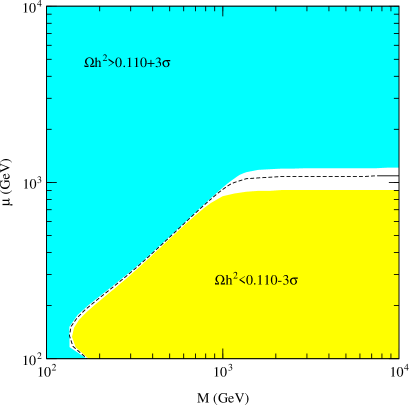
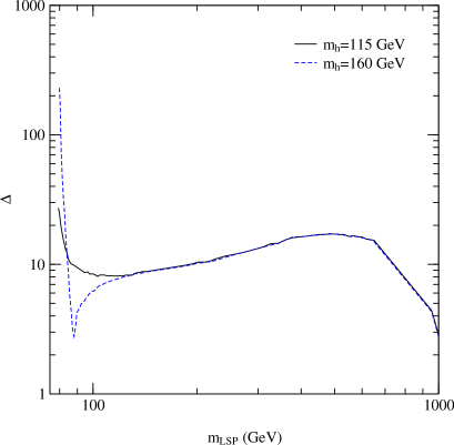
Figure 1: Left Panel: In white, the WMAP 3-$\sigma$ allowed region in the plane $(M,\,\mu)$; the dashed line shows the isolevel curve with $\Omega h^{2}=0.110$. $m_{h}$ is assumed to be equal to 160 GeV. Right Panel: Fine-tuning parameter $\Delta$ versus lightest neutralino mass for models with thermal relic abundance $\Omega h^{2}=0.110$. The two sample values for $m_{h}$ are displayed, featuring (or avoiding) an s-channel resonance in the LSP pair annihilation rate.

In the left panel of Fig. 1 we plot the region of the plane $(M,\,\mu)$ with relic density of the LSP matching the WMAP preferred value for $\Omega h^{2}$ (0.110 along the dashed line and within $3\sigma$ in the white region). There are two interesting regimes: in the first one, at $M>>\mu$, the lightest neutralino is an almost pure Higgsino and its thermal relic abundance is set by the pair annihilation rate into gauge bosons, with coannihilations with the next-to-lightest neutralino and the chargino playing an important role. In this regime the LSP mass is essentially equal to $\mu$ and imposing $\Omega h^{2}=0.110$, one finds $\mu\simeq 1.1~{}{\rm TeV}$. The second interesting region starts at $M\sim\mu\sim 1~{}{\rm TeV}$ and extends down to small $M$ and $\mu$, along the diagonal in the plot. For these models the LSP has a large gaugino-Higgsino mixing, while the mass splitting with the next-to-lightest neutralino and the chargino gets larger. In this regime the thermal relic abundance is set by the pair annihilation rate into gauge bosons and coannihilation with chargino which get less and less relevant. For a given LSP mass, a tuning on the LSP Higgsino fraction (and consequently on the LSP pair annihilation rate into gauge bosons) is then needed to recover the correct relic abundance. The plot is obtained for $\tan\beta=30$ and $m_{h}\sim 160\,{\rm GeV}$. Changing $\tan\beta$ does not affect out results, since it does not change the Higgsino fraction. The SM-like Higgs boson mediates the s-channel annihilation of LSP’s into a fermion-antifermion pair; this process is subdominant except when close to the s-cahnnel resonance, i.e. for $m_{LSP}\sim m_{h}/2$. In the plot this takes place at a LSP mass of $\sim$ 80 GeV (the turnaround at the lower-left corner in the plot); if we shift $m_{h}$ to a lower value, say the current limit on the SM-like Higgs mass $\sim$ 115 GeV [18], the cosmologically preferred region is essentially unchanged, since 80 GeV is anyhow the threshold for $W$-boson final states, while at the resonant mass a very tiny slice of the parameter space becomes allowed (the $h$-Higgs boson has a very small width, about 0.3 GeV). In the regime at large Bino-Higgsino mixing, the $3\sigma$ WMAP-allowed region is very narrow; in the right panel of Fig. 1 we plot, versus LSP mass and for models with relic density $\Omega h^{2}=0.110$, the fine-tuning parameter $\Delta$, defined as:

$$\Delta=\sqrt{\sum_{i}\left|d\log(\Omega h^{2})\over d\log x_{i}\right|^{2}}$$ (5)

where the sum is over the two $x_{i}$ parameters $\mu$ and $M$. Moderate values of $\Delta$ (say $\stackrel{{\scriptstyle<}}{{{}_{\sim}}}10$) can be obtained. For pure Higgsinos the fine tuning is very small, while it gets large for models that have, at the same time, large mixing and relic density dominated by coannihilation effects (largest sensitivity on the tuning of the Higgsino fraction). The peak in $\Delta$ at the LSP low mass end is due either to the $W$-boson threshold effect or, specially, to the $h$ resonance.

In the discussion on DM detection rates we will make predictions also for models that are outside the $3\sigma$ WMAP preferred region, still under the assumption that they account for the dark matter in the Universe. The reason for such a choice is that the results we have shown are not totally general: a few assumptions on the particle physics and cosmological model are involved and, if they are relaxed, the value of the relic density may either increase or decrease. E.g., there could be extra non-thermal sources on top of the thermal component; the Universe expansion rate at freeze out could be faster than the value extrapolated according to the SM particle content, or there could be injections of entropy at late times diluting the thermal relic density component. Effects of this kind have been discussed, e.g. in [19].

4 Detection rates

A very strong experimental effort is currently devoted to searches for dark matter in the form of weakly interactive massive particles (WIMPs), see, e.g. Ref. [20] for a review. We discuss here techniques which are relevant for the LSP in the present framework. All predictions are obtained with an appropriate interface of the model to the DarkSUSY package.

4.1 Direct detection

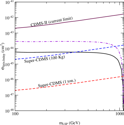
Figure 2: Lightest neutralino spin independent cross section per nucleon versus lightest neutralino mass, for models with $\Omega h^{2}=0.110$. The solid line corresponds to the case of $m_{h}=160\,\rm{GeV}$, while the dash-dotted line to models with $m_{h}=115\,\rm{GeV}$. Also the current limit from the CDMS experiment [22] and future projected sensitivities are shown.

The goal of WIMP direct searches is to measure the energy deposited through elastic scatterings with nuclei by DM WIMP’s passing through the target material of a detector [21]. Several complementary approaches have been developed to optimize signal versus backgrounds. In general for neutralinos, as for any Majorana fermion, two terms can contribute to the scattering cross section: the axial-vector spin-dependent (SD) coupling, and the scalar spin-independent (SI) term, which is coherent and tends to dominate for materials made out of heavy nuclei. In particular in a split SUSY scenario the LSP-nucleon SD and SI couplings can only be mediated by the $Z$ boson and a CP-even Higgs in a t-channel, respectively, since all squark contributions are suppressed by the fact that squarks are very heavy. As already pointed out in Section 2, at tree-level, the vertex $Z$-LSP-LSP vanishes, hence the SD scattering cross-section is always extremely small. In Fig. 2 we present predictions for the SI neutralino-proton scattering cross-section, versus lightest neutralino mass and for the model with relic density $\Omega h^{2}=0.110$ (standard values for nucleonic matrix elements are assumed, see [17]). The results are proportional to $1/m_{h}^{4}$ and they are sensitive to the Bino-Higgsino mixing since the $h$-LSP-LSP vertex is proportional to it. The conspiracy of the previous effects takes into account the sudden fall of the SI cross section in Fig. 2, having in mind that higher values of LSP mass imply a small mixing between Binos and Higgsinos as shown in Fig. 1. Also shown in Fig. 2 are the current best limit on the WIMP-nucleon SI cross-section from the CDMS collaboration [22] and projected sensitivities of upcoming larger-mass detectors, such as the SuperCDMS [23] (expectations for other projects with comparable masses are analogous). No model in our framework is excluded by current constraints; note however that a very large portion of the parameter space will be tested at future facilities. This is even more evident from the left panel of Fig. 3, where future projected sensitivities are plotted in the $\mu-M$ plane: the whole regime with mass parameters below about 1 TeV will be probed (conservatively, $m_{h}$ was set equal to 160 GeV).

 

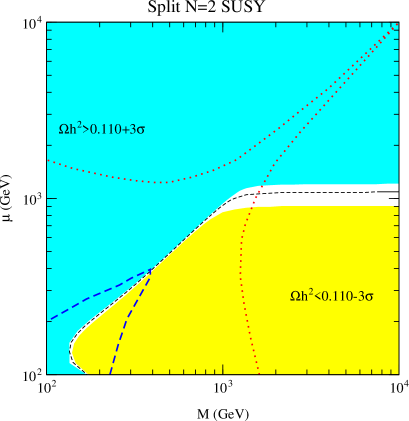
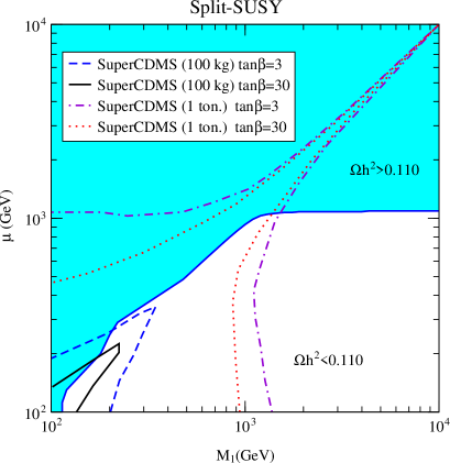
Figure 3: Left Panel: Projected future sensitivities of the SuperCDMS experiment in the $(M,\,\mu)$ plane for our split $N=2$ SUSY model; the dotted line corresponds to the 1 ton configuration, the dashed line to the 100 kg setup. Results are not sensitive to $\tan\beta$. Right Panel: Sensitivity curves in the $(M_{1},\,\mu)$ plane for a split SUSY model within the standard MSSM setup; two sample values of $\tan\beta$ are considered. In both frameworks $m_{h}=160\,\rm{GeV}$ is assumed.

In the right panel of Fig. 3 we sketch the analogous picture in the case of a split spectrum within the standard MSSM; here $M_{1}$ is the mass parameter for the (single) bino, while it has been assumed that the wino mass parameter $M_{2}$ is much heavier than $M_{1}$ and $\mu$ (see [5] for details). While trends are similar, there are a few significant differences: the departure from the diagonal of the $\Omega h^{2}=0.110$ isolevel curve is due to the $t\bar{t}$ final state which becomes kinematically allowed at $M_{1}\sim\mu\sim 200$ GeV and it is mediated by a $Z$ boson in the s-channel (the vertex $Z$-LSP-LSP is not zero in this case). Moreover the SI scattering cross section depends on $\tan\beta$, since this intervene in determining the LSP Bino-Higgsino mixing: from moderate to large values of $\tan\beta$ the region in the parameter space accessible to future searches shrinks, and it is in all cases less extended than the corresponding region for our split extended SUSY framework, which does not depend on $\tan\beta$ because of the two-Bino construction.

4.2 Indirect searches with neutrino telescopes

Since WIMP’s have a (small) coupling to ordinary matter, they can get trapped in the potential well of massive celestial bodies, sink in the center of the system and build up a dense WIMP population which in turn can give rise to a neutrino flux. This effect has been studied in detail for the Sun and the Earth [20] and, roughly speaking, the trend one sees is that detectable fluxes are obtained only for models for which capture and annihilation rates reach equilibrium (or are close to it).

In particular, the capture rate in the Sun is efficient if the SD scattering cross section is sizable. As already mentioned in our framework the SD coupling is negligible and we find that the SI one does not compensate for it. We find predictions for neutrino fluxes which are always well below the expected sensitivity of future km³ size telescopes, such as IceCube [24]. This is in contrast to what one finds for split models within the MSSM [5]. In the latter case the SD coupling is not suppressed and a detectable neutrino signal is expected for models with large gaugino-Higgsino mixing and mass up to about 500 GeV; this could be in principle exploited to discriminate between our framework and the standard scenario. In case of the Earth, the SI coupling is the relevant effect; however we still find that the predicted neutrino fluxes are too small.

4.3 Indirect searches through cosmic- and gamma-rays

 

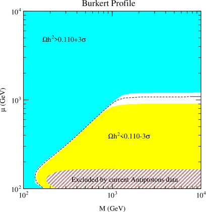
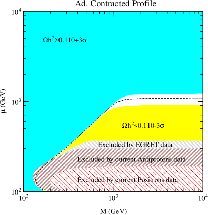
Figure 4: Limits on the model from the available measurements of the local antimatter flux and from the gamma-ray flux measured by EGRET towards the center of the Galaxy, in case of the Burkert halo profile (left panel) and the adiabatically contracted profile (right panel).

If WIMP’s are indeed the building blocks of all structures in the Universe, they would populate the Milky Way halo as well, and their pair annihilation could give rise to detectable yields. The focus is on species with small or well-determined background from standard sources, such as antimatter components, i.e. antiprotons, positrons and antideuterons, and gamma-rays. In order to make predictions for the induced fluxes we need to simulate for the fragmentation and/or decay processes for each final state of LSP annihilations to estimate the energy distribution of these yields. This is done in the DarkSUSY package by linking to simulations performed with the Pythia [25] Monte Carlo code, except for the $\bar{D}$ source for which the prescription suggested in Ref. [26] is implemented.

Since source functions scale with the square of the LSP density locally in space, the induced fluxes will be sensitive to the distribution of LSP’s in the halo. We will refer to two opposite configurations: i) A Burkert profile [27], which has a large core and hence a constant density in its inner region, essentially from our position in the Galaxy inward; and ii) A profile matching the results from N-body simulation of cold DM [28], i.e. a profile with a sharp enhancement in the density towards the center of the system, as reshaped from the infall of the baryonic components of the Milky Way in the adiabatic contraction limit [29] . The spread in the predictions we will show for the two configurations will give a feeling for the uncertainty in the predictions related to the halo model. Even in the case of the second model, we are not considering the most favorable scenario; including, e.g. effects due the presence of substructures would give a further enhancement in the predictions.

To make predictions on antimatter fluxes one further step has to be considered, in particular the simulation of the propagation of charged particles in galactic magnetic fields. We use the two dimensional diffusion model developed in Refs. [33, 34], as included in the DarkSUSY package, with a set of propagation parameters which was shown to reproduce fairly well the ratios of primary to secondary cosmic ray nuclei [35] with the Galprop [36] propagation code in the diffusion/convection limit. Solar modulation is instead sketched with the analytical force-field approximation [37], with a modulation parameter as appropriate at each phase in the solar cycle activity.

In Fig. 4 we show current limits on the split $N=2$ SUSY model from the available measurements of the local antiproton and positron cosmic-ray fluxes [38, 39], for the two halo models we are considering. The limits are derived at $3\sigma$ with a $\chi^{2}$ discrimination procedure, taking a standard prediction for the background and neglecting uncertainties on it. For the Burkert profile we do not have any constraint from positrons and gamma-rays flux measurements while antiproton data do not exclude any model on the $\Omega h^{2}=0.110$ isolevel curve. For the adiabatically contracted case low mass models with thermal relic abundance in agreement with WMAP data tend to give a too large antiproton flux while also positron flux measurement rules out a corner in the plane $(M,\mu)$. Furthermore, in this second case a part of the parameter space is also excluded because it gives a gamma-ray flux which is larger than the flux measured by the EGRET gamma-ray telescope towards the Galactic Center [40]. More recent data at higher energy from the HESS [41] and MAGIC [42] telescopes give less tight constraints.

 

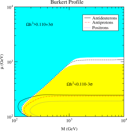
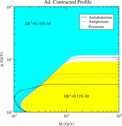
Figure 5: Portions of the parameter space which will be tested by the Pamela and GAPS measurements of the antiproton, positron and antideuteron fluxes in case of the Burkert halo profile (left panel) and the adiabatically contracted profile (right panel).

Very recently the PAMELA satellite experiment [43] has been launched. In the next few years very high quality data on the antiproton and positron fluxes will be available, allowing for a better discrimination of a component from WIMP annihilations. In Fig. 5 we show the regions in the parameter space which will be tested by Pamela in three years of data taking (the extrapolation on these sensitivity curves is done following the approach described in Ref. [44]). We also show the prospects for indirect detection with antideuteron searches obtained by comparing the predicted flux with the estimated sensitivity of the planned gaseous antiparticle spectrometer (GAPS) [45], about $2.6\times 10^{-9}\textrm{m}^{-2}\textrm{sr}^{-1}\textrm{GeV}^{-1}\textrm{s}^{-1}$ in the 0.1-0.4 GeV energy range . All indirect signals scale with the pair annihilation cross section, which is large for pure Higgsinos and get very small for pure Binos; it is inversely proportional to the square of the LSP mass. The dominant annihilation channels are gauge boson final states, which are copious sources of antiprotons and positrons, and which tend to give LSP signals with very distinctive features, see e.g. the ”W-boson bump” discussed in [34] for the positron flux. The shift in the sensitivity curves going from the case with LSP distribution described by the Burkert profile to the adiabatically contracted case is very large and differs in the three detection channels; this is due to the fact that spatial propagation is rather efficient for antiprotons, while antideutrons are more fragile and positrons lose energy on a shorter timescale. The relative weight of the three states is also changing with the value of LSP mass, with the antideuteron yield getting suppressed for heavier neutralinos.

Finally, comparing the perspectives for halo signals with those for direct detection in Fig. 3, one can see that there is complementarity between the region of the parameter space probed by indirect detection and the one accessible to direct searches; in this respect, the result of this analysis is analogous to what was found for split SUSY models within the MSSM framework, see [5].

5 Conclusion

We have discussed the dark matter phenomenology for a split SUSY model arising from a high energy intersecting brane model with $N=2$ supersymmetry. Its active states at low energy differ from those in the standard split SUSY scenario based on the MSSM. Analogies and differences compared to the standard case have emerged. In both frameworks the lightest neutralino is a dark matter candidate for: i) Intermediate mass neutralinos with a sizable Bino-Higgsino mixing, or ii) A pure Higgsino state at the TeV scale. The fine-tuning parameter for such configurations is in general rather small. In the split $N=2$ SUSY model direct detection is very promising, covering a significantly larger portion of the parameter space than in the standard case; in particular all results in the present analysis are essentially independent of $\tan\beta$, and the spin independent scattering cross section does not get suppressed in the large $\tan\beta$ limit as in the MSSM. Concerning indirect detection searches with neutrino telescopes are not relevant in this specific extended SUSY scenario, while antimatter measurements have already excluded a relevant portion of the parameter space. In the next few years the Pamela detector will measure the antiproton and positron fluxes with higher accuracy, allowing for further tests of the model in a regime which is complementary to direct detection searches.

References

- [1] D. N. Spergel et al., arXiv:astro-ph/0603449.
- [2] N. Arkani-Hamed and S. Dimopoulos, JHEP 0506 (2005) 073 [arXiv:hep-th/0405159].
- [3] G. F. Giudice and A. Romanino, Nucl. Phys. B 699 (2004) 65 [Erratum-ibid. B 706 (2005) 65] [arXiv:hep-ph/0406088].
- [4] K. Griest and M. Kamionkowski, Phys. Rev. Lett. 64 (1990) 615.
- [5] A. Masiero, S. Profumo and P. Ullio, Nucl. Phys. B 712 (2005) 86 [arXiv:hep-ph/0412058].
- [6] N. Arkani-Hamed, S. Dimopoulos, G. F. Giudice and A. Romanino, Nucl. Phys. B 709 (2005) 3 [arXiv:hep-ph/0409232].
- [7] I. Antoniadis and S. Dimopoulos, Nucl. Phys. B 715 (2005) 120 [arXiv:hep-th/0411032].
- [8] B. Kors and P. Nath, Nucl. Phys. B 711 (2005) 112 [arXiv:hep-th/0411201].
- [9] K. S. Babu, T. Enkhbat and B. Mukhopadhyaya, Nucl. Phys. B 720 (2005) 47 [arXiv:hep-ph/0501079].
- [10] B. Dutta and Y. Mimura, Phys. Lett. B 627 (2005) 145 [arXiv:hep-ph/0503052].
- [11] I. Antoniadis, A. Delgado, K. Benakli, M. Quiros and M. Tuckmantel, Phys. Lett. B 634 (2006) 302 [arXiv:hep-ph/0507192]; I. Antoniadis, K. Benakli, A. Delgado, M. Quiros and M. Tuckmantel, Nucl. Phys. B 744 (2006) 156 [arXiv:hep-th/0601003].
- [12] A. Pierce, Phys. Rev. D 70 (2004) 075006 [arXiv:hep-ph/0406144].
- [13] A. Arvanitaki and P. W. Graham, Phys. Rev. D 72 (2005) 055010 [arXiv:hep-ph/0411376].
- [14] L. Senatore, Phys. Rev. D 71 (2005) 103510 [arXiv:hep-ph/0412103].
- [15] N. Arkani-Hamed, A. Delgado and G. F. Giudice, Nucl. Phys. B 741 (2006) 108 [arXiv:hep-ph/0601041].
- [16] L. Alvarez-Gaume and S. F. Hassan, Fortsch. Phys. 45 (1997) 159 [arXiv:hep-th/9701069].
- [17] P. Gondolo, J. Edsjo, P. Ullio, L. Bergstrom, M. Schelke and E. A. Baltz, JCAP 0407 (2004) 008 [arXiv:astro-ph/0406204].
- [18] W.-M. Yao et al., J. Phys. G 33 (2006) 1.
- [19] M. Kamionkowski, K. Griest, G. Jungman and B. Sadoulet, Phys. Rev. Lett. 74 (1995) 5174; T. Moroi and L. Randall, Nucl. Phys. B 570 (2000) 455 [arXiv:hep-ph/9906527]; M. Fujii and K. Hamaguchi, Phys. Lett. B 525 (2002) 143 [arXiv:hep-ph/0110072]; P. Salati, Phys. Lett. B 571 (2003) 121; S. Profumo and P. Ullio, JCAP 0311 (2003) 006 [arXiv:hep-ph/0309220].
- [20] L. Bergstrom, New Astron. Rev. 42 (1998) 245.
- [21] M. W. Goodman and E. Witten, Phys. Rev. D 31 (1986) 3059; I. Wasserman, Phys. Rev. D 33 (1986) 2071.
- [22] D. S. Akerib et al. [CDMS Collaboration], Phys. Rev. Lett. 96 (2006) 011302 [arXiv:astro-ph/0509259].
- [23] D. S. Akerib et al., Nucl. Instrum. Meth. A 559 (2006) 411.
- [24] A. Achterberg et al. [IceCube Collaboration], arXiv:astro-ph/0509330.
- [25] T. Sjöstrand, Comput. Phys. Commun. 82 (1994) 74. ; T. Sjöstrand, PYTHIA 5.7 and JETSET 7.4. Physics and Manual, CERN-TH.7112/93, arXiv:hep-ph/9508391 (revised version).
- [26] F. Donato, N. Fornengo and P. Salati, Phys. Rev. D62 (2000) 043003.
- [27] A. Burkert, Astrophys. J. 447 (1995) L25.
- [28] J.F. Navarro et al., MNRAS 349 (2004) 10039.
- [29] G.R. Blumental, S.M. Faber, R. Flores and J.R. Primack, Astrophys. J. 301 (1986) 27.
- [30] P. Ullio, H.S. Zhao and M. Kamionkowski, Phys. Rev. D 64 (2001) 043504.
- [31] D. Merritt, M. Milosavljevic, L. Verde and R. Jimenez, Phys. Rev. Lett. 88 (2002) 191301.
- [32] J. Edsjo, M. Schelke and P. Ullio, JCAP 0409 (2004) 004 [arXiv:astro-ph/0405414].
- [33] L. Bergström, J. Edsjö and P. Ullio, Astrophys. J. 526 (1999) 215.
- [34] E.A. Baltz, J. Edsjo, Phys. Rev. D59 (1999) 023511.
- [35] I.V. Moskalenko, A.W. Strong, J.F. Ormes and M.S. Potgieter, Astrophys. J. 565 (2002) 280.
- [36] Galprop numerical package, http://www.mpe.mpg.de/~aws/propagate.html.
- [37] L.J. Gleeson and W.I. Axford, Astrophys. J. 149 (1967) L115.
- [38] S. Orito et al., Phys. Rev. Lett. 84 (2000) 1078; Y. Asaoka et al., Phys. Rev. Lett. 88 (2002) 05110; Boezio et al., Astrophys. J. 561 (2001) 787.
- [39] DuVernois et al., Astrophys. J. 559 (2001) 296; Boezio et al., Astrophys. J. 532 (2000) 653; H. Gast, J. Olzem and S. Schael, arXiv:astro-ph/0605254.
- [40] H.A. Mayer-Hasselwander et al., Astron. Astrophys. 335 (1998) 161.
- [41] F. Aharonian et al., Astron. Astrophys. 425 (2004) L13.
- [42] J. Albert et al., Astrophys. J. 638 (2006) L101.
- [43] O. Adriani et al. (Pamela Collaboration), Proc. of the 26th ICRC, Salt Lake City, 1999, OG.4.2.04.
- [44] S. Profumo and P. Ullio, JCAP 0407 (2004) 006 [arXiv:hep-ph/0406018].
- [45] K. Mori, C. J. Hailey, E. A. Baltz, W. W. Craig, M. Kamionkowski, W. T. Serber and P. Ullio, Astrophys. J. 566 (2002) 604 [arXiv:astro-ph/0109463].