Renormalized Finite Temperature $\mathbf{\phi^{4}}$ theory from the 2PI Effective Action

Abstract

We present a numerical and analytical study of scalar $\phi^{4}$ theory at finite temperature with a renormalized 2-loop truncation of the 2PI effective action.

1 Introduction

The thermodynamical properties of a physical system can be extracted from the effective potential, which is given as a function $\gamma[\phi]$ of a condensate field $\phi$. In the thermodynamic limit, its stationary point defines the free energy $\mathcal{F}$ as

$$\mathcal{F}=\lim_{V\rightarrow\infty}\gamma[\bar{\phi}],\quad\mbox{with}\quad\frac{\delta\gamma[\phi]}{\delta\phi}\Big{|}_{\phi=\bar{\phi}}=0.$$ (1)

Once the free energy is known, all other thermodynamic quantities, such as the entropy or energy density, can be easily derived. At finite temperature collective phenomena are known to modify substantially the properties of the elementary excitations, so the use of a perturbative expansion around the free theory to calculate the effective potential becomes questionable and often leads to inconsistencies. One needs then to consider nonperturbative schemes. For situations where the effects of the collective phenomena can be conveniently captured by a suitable modification of the 2-point functions, resummation schemes based on the 2PI effective action can be very useful [2]. The 2PI effective action provides a reorganization of the perturbative expansion around dressed 2-point functions, which are determined self-consistently for a given approximation/truncation. In this work we study the thermodynamics of scalar $\phi^{4}$ theory using a 2-loop truncation of the 2PI effective action.

2 2-loop truncation of the 2PI effective action

For scalar $\phi^{4}$ theory the 2PI effective action can be parametrized as [1]

$$\Gamma_{\mbox{\scriptsize 2PI}}[\phi,G]=\frac{1}{2}\phi\cdot G_{0}^{-1}\cdot\phi+\frac{1}{2}\mbox{Tr}\big{[}\mbox{ln}G^{-1}+\left(G_{0}^{-1}-G^{-1}\right)\cdot G\big{]}+\Gamma_{{\mbox{\scriptsize int}}}[\phi,G],$$ (2)

with $\phi$ and $G$ generic 1- and 2-point functions and $A\cdot B$ a shorthand notation for the convolution of $A$ and $B$. The term $\Gamma_{{\mbox{\scriptsize int}}}$ contains the interactions and can be written as an expansion in terms of two-particle-irreducible (2PI) diagrams. Up to 2-loops it is given by

$$-\Gamma_{\mbox{\scriptsize int}}[\phi,G]=\frac{1}{4!}\;\parbox[c]{20.0pt}{\begin{picture}(20.0,30.0)(0.0,0.0) \put(0.0,0.0){} \put(0.0,0.0){} \put(0.0,0.0){} \put(0.0,0.0){} \put(0.0,0.0){} \put(0.0,0.0){} \put(0.0,0.0){} \put(0.0,0.0){} \put(0.0,0.0){} \put(0.0,0.0){} \put(0.0,0.0){} \put(0.0,0.0){} \put(0.0,0.0){} \end{picture}}\;+\frac{1}{4}\;\parbox[c]{20.0pt}{\begin{picture}(20.0,30.0)(0.0,0.0) \put(0.0,0.0){} \put(0.0,0.0){} \put(0.0,0.0){} \put(0.0,0.0){} \put(0.0,0.0){} \put(0.0,0.0){} \put(0.0,0.0){} \put(0.0,0.0){} \end{picture}}\;+\frac{1}{8}\;\parbox[c]{20.0pt}{\begin{picture}(20.0,30.0)(0.0,0.0) \put(0.0,0.0){} \put(0.0,0.0){} \put(0.0,0.0){} \end{picture}}\;+\frac{1}{12}\;\parbox[c]{45.0pt}{\begin{picture}(45.0,30.0)(0.0,0.0) \put(0.0,0.0){} \put(0.0,0.0){} \put(0.0,0.0){} \put(0.0,0.0){} \put(0.0,0.0){} \put(0.0,0.0){} \put(0.0,0.0){} \put(0.0,0.0){} \put(0.0,0.0){} \put(0.0,0.0){} \end{picture}}\;$$ (3)

Within the approximation, “physical” 1- and 2-point functions $\bar{\phi}$ and $\bar{G}$ are determined self-consistenly as the stationary points of the 2PI effective action, i.e.

$$\frac{\delta\Gamma_{\mbox{\scriptsize 2PI}}}{\delta G}\Big{|}_{\bar{G}[\phi],\phi}=0\quad\mbox{and}\quad\frac{\delta\Gamma_{\mbox{\scriptsize 2PI}}}{\delta\phi}\Big{|}_{\bar{G}[\phi],\bar{\phi}}=0.$$ (4)

The stationary conditions (4) turn into a set of coupled implicit equations for ${\bar{G}}$ and $\bar{\phi}$ which have to be solved in order to calculate any physical quantity. In particular, the knowledge of the dressed 2-point function $\bar{G}$ allows one to calculate the effective potential as $\gamma[\phi]=TV^{-1}\Gamma_{{\mbox{\scriptsize 2PI}}}[\phi,\bar{G}[\phi]]$.

One of the main complications that arises when dealing with truncations of the 2PI effective action is the fact that 2- and higher $n$-point functions are not uniquely defined [4]. In particular, a given truncation defines two possible 2-point functions and three 4-point functions. One of the 2-point functions is given by the stationary value $\bar{G}$, while the other is related to the inverse curvature of the effective potential as $\hat{G}^{-1}=TV^{-1}\left[\delta^{2}\gamma[\phi]/\delta\phi^{2}\right]$. The three 4-point functions and their corresponding vertices are given in terms of coupled Bethe-Salpeter-like equations [4]. Concerning renormalization, the ambiguity in the definition of the vertex functions implies that there are more than one counterterm of a given type [3]. A given counterterm is determined by applying a renormalization condition to the corresponding vertex. For consistency, identical renormalization conditions are applied to all counterterms of the same type. It is simpler to consider renormalization conditions applied at a reference temperature $T_{\star}$ for which the physical field configuration is $\bar{\phi}_{\star}=0$. This requires that $T_{\star}>T_{c}$ if a critical temperature $T_{c}$ exists. Defining the self-energy from Dyson’s equation $\bar{\Sigma}={\bar{G}}^{-1}-G_{0}^{-1}$, the renormalized equations for $\bar{\Sigma}$ and $\bar{\phi}$ are

$$\bar{\Sigma}(P) =\delta m_{0}^{2}+\frac{\lambda+\delta\lambda_{2}}{2}\phi^{2}+\frac{\lambda+\delta\lambda_{0}}{2}\int_{K}^{T}\bar{G}(K)-\frac{\lambda^{2}}{2}\phi^{2}\Theta(P)$$ (5)

$$\left(m^{2}+\delta m_{2}^{2}\right){\bar{\phi}} =\frac{\lambda+\delta\lambda_{4}}{6}{\bar{\phi}}^{3}+\frac{\lambda+\delta\lambda_{2}}{2}{\bar{\phi}}\int_{K}^{T}{\bar{G}}(K)-\frac{\lambda^{2}}{6}{\bar{\phi}}\int_{K}^{T}{\bar{G}}(K)\Theta(K),$$ (6)

with $\smash{\int_{K}^{T}}$ a short-hand notation for the standard sum-integral over momentum $K$ at temperature $T$, and $\smash{\Theta(P)=\int_{K}^{T}{\bar{G}}(K){\bar{G}}(K+P)}$. The bar in $\phi$ has been omitted in the first equation to stress the fact that it can be solved for any value. This is needed, for instance, to calculate the effective potential $\gamma[\phi]$. The explicit expressions for the counterterms $\delta m_{0}^{2}$, $\delta m_{2}^{2}$, $\delta\lambda_{0}$, $\delta\lambda_{2}$ and $\delta\lambda_{4}$ can be found in Ref. [4]. With those counterterms it can be shown that, for any value of $T$ and $\phi$, the results for ${\bar{G}}$, ${\bar{\phi}}$ and $\gamma[\phi]$ are UV-finite.

3 Numerical Analysis

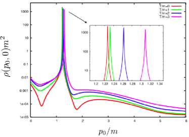
The gap and field equations (5) and (6) are solved numerically in Minkowski space. We split the self-energy into a local and a non-local part as $\bar{\Sigma}(P)=\bar{\Sigma}^{l}+\bar{\Sigma}^{nl}(P)$. The momentum dependent part is expanded in both $p_{0}$ and $|\mathbf{p}|$ using $N$ Chebyshev polynomials as $\smash{\bar{\Sigma}^{nl}(p_{0},|\mathbf{p}|)=\sum_{i}^{N}\sum_{j}^{N}c_{ij}T_{i}(p_{0})T_{j}(|\mathbf{p}|)}$. The solution to the gap and field equations is obtained by solving the matrix equation for the $N^{2}$ coefficients $c_{ij}$ plus the local terms $\Sigma^{l}$ and/or ${\bar{\phi}}^{2}$ by means of a multi-dimensional Newton-Raphson method. This numerical algorithm is fairly stable and converges after few iterations. For a given $N$, the numerical solution oscillates around the “full” solution, which is convenient for the calculation of integrated quantities, such as the effective potential. Unlike lattice-based methods, this technique also allows the use of large (small) UV (IR) cut-offs, which is useful for the study of renormalization and/or critical phenomena. Although numerically more expensive, the advantage of solving the equations in Minkowski space is that one can obtain directly spectral properties of the system without the need of analytic continuation. In particular, the spectral function $\rho(p_{0},\mathbf{|p|})$ can be constructed from the knowledge of the real and imaginary parts of the retarded self-energy, which come directly from solving equation (5) (see Fig. 1 for an example result at several temperatures). The width, the position of the quasiparticle pole and the effect of multiparticle contributions can be adequately studied with the presented algorithm.

Figure 1: Spectral function $\rho(p_{0},0)$ for $\lambda=1$, $\phi/m=1$ and $T_{\star}/m=1$ and several temperatures.

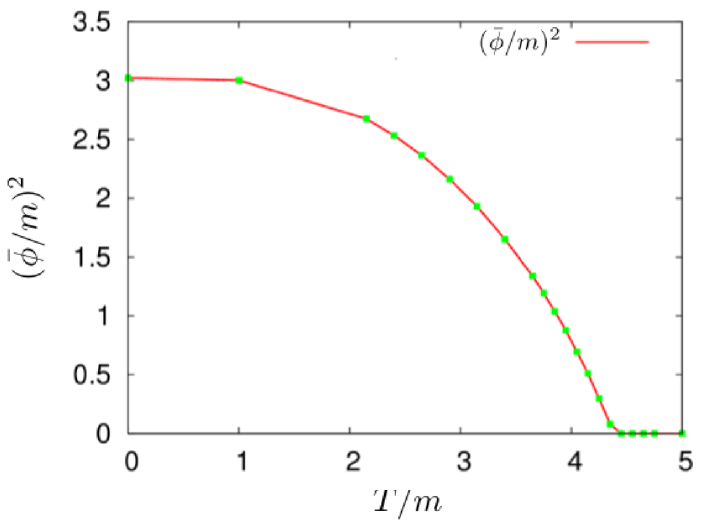
We can also look at the critical behaviour in a system with broken symmetry. A simple quantity to compute is the critical temperature which can be read off the 2-point functions at vanishing effective mass $M$. As we discussed previously there are two possible 2-point functions (${\bar{G}}$ and $\hat{G}$), for which the corresponding effective masses are (in the symmetric phase)

$$M^{2}(T,\lambda) =m^{2}+\Sigma^{l}(T,\lambda),$$ (7)

$$\hat{M}(T,\lambda) =\hat{G}^{-1}(p=0,T,\lambda)=\frac{\delta^{2}\Gamma[\phi,{\bar{G}}[\phi]]}{\delta\phi^{2}}\Big{|}_{{\bar{\phi}}}(p=0,T,\lambda).$$ (8)

Starting from $T_{\star}$ and reducing the temperature, the critical values $T_{c}$ and $\hat{T}_{c}$ are found when $M^{2}(T_{c},\lambda)$ and $\hat{M}(\hat{T}_{c},\lambda)$ vanish (see Fig. 2, left). We can also vary the UV-cutoff in the calculation of the critical temperatures and therefore check the validity of the renormalization procedure (see Fig. 2, right). We find that both quadratic and logarithmic divergences (present respectively in $T_{c}$ and $\hat{T}_{c}$) are properly renormalized and hence the renormalization is satisfactory.

\psfrag{DOT}{\tiny$\hat{T}_{c}/m$}\psfrag{GOT}{\tiny$T_{c}/m$}\includegraphics[width=368.57964pt]{./pictures/tcvsl.eps}

\psfrag{POT}{\tiny$\hat{T}_{c}/m$}\psfrag{ROT}{\tiny$T_{c}/m$}\includegraphics[width=368.57964pt]{./pictures/cutoffdependence.eps}

Figure 2: Left: Critical temperatures for several couplings and $T_{\star}/m=5$. Right: UV cut-off dependence for $\lambda=3$.

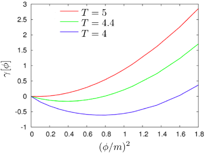
Solving in addition the field equation (6) allows us to study the phase transition (see Fig. 3, left). We see the transition is clearly of second order. A similar conclusion is reached by computing directly the effective potential $\gamma[\phi]$ (see Fig. 3, left). We checked that $\gamma[{\bar{\phi}}]$, from which a renormalized free energy and pressure can be extracted, is cutoff independent.

Figure 3: Left: field expectation value ${\bar{\phi}}^{2}$ as a function of $T$ for $\lambda=3$ and $T_{\star}/m=5$. Right: Effective potential.

References

• [1] J. M. Cornwall, R. Jackiw and E. Tomboulis, Phys. Rev. D10 2428-2445 (1974).
• [2] B. Vanderheyden and G. Baym, J. Stat. Phys. 93, 843 (1998); J.-P. Blaizot, E. Iancu and A. Rebhan, Phys. Rev. Lett.  83, 2906 (1999); J. T. Lenaghan and D. H. Rischke, J. Phys. G 26, 431 (2000). Y. Nemoto, K. Naito and M. Oka, Eur. Phys. J. A 9 (2000) 245 Phys. Rev. D 63, 065003 (2001). J. Berges, Sz. Borsányi, U. Reinosa and J. Serreau, Phys. Rev. D71, 105004 (2005). J.-P. Blaizot, A. Ipp, A. Rebhan, U. Reinosa, Phys. Rev. D72, 125005 (2005). D. Roder, J. Ruppert and D. H. Rischke, arXiv:hep-ph/0503042. D. Roder, arXiv:hep-ph/0509232.
• [3] J. Berges, Sz. Borsányi, U. Reinosa and J. Serreau, Annals Phys. 320, 344-398 (2005).
• [4] A. Arrizabalaga and U. Reinosa, in preparation.