DESY 06-154
SFB/CPP-06-40
Planar two-loop master integrals for massive Bhabha scattering:
$N_{f}=1$ and $N_{f}=2$

Abstract

Recent developments in the computation of two-loop master integrals for massive Bhabha scattering are briefly reviewed. We apply a method based on expansions of exact Mellin-Barnes representations and evaluate all planar four-point master integrals in the approximation of small electron mass at fixed scattering angle for the one-flavor case. The same technique is employed to derive and evaluate also all two-loop masters generated by additional fermion flavors. The approximation is sufficient for the determination of QED two-loop corrections for Bhabha scattering in the kinematics planned to be used for the luminosity determination at the ILC.

1 Introduction

Bhabha scattering is the process employed to measure the luminosity at electron-positron colliders, because of its clear experimental signature. At machines operating at a $1-10$ $\rm{GeV}$ centre-of-mass energy $\sqrt{s}$, the relevant kinematic region is that of large-angle Bhabha scattering. Small-angle Bhabha scattering, instead, is an invaluable luminosity monitor at high-energy colliders in the TeV region.

In order to minimize the luminosity error, a precise theoretical computation of radiative corrections to the Bhabha-scattering cross section is required. The electroweak next-to-leading order (NLO) corrections to Bhabha scattering were computed a long time ago in [1]. In recent years, studies have been focusing on pure quantum electrodynamics (QED) contributions beyond the one-loop level. The two-loop virtual corrections for massless electrons were obtained in [2]. However, this result was not immediately useful since the available Monte Carlo programs employ a non-vanishing electron mass $m$.

The virtual and real second-order contributions to Bhabha scattering, enhanced by factors of $\ln(s/m^{2})$ and $\ln^{2}(s/m^{2})$ were completed in [3, 4, 5, 6]. This result was recently improved in [7, 8, 9], where the photonic non-logarithmic term was evaluated at leading order in the ratio $m^{2}/s$. The diagrams with fermion loops remained uncovered in this approach.

An important breakthrough in the field was the use of the Laporta-Remiddi algorithm ([10, 11]), in order to reduce the Bhabha-scattering cross section to a few Master Integrals (MIs). The technique of differential equations proved useful in evaluating several MIs (see i.e. [12, 13, 14]). The results were represented in terms of Harmonic Polylogarithms (HPLs) introduced in [15] or of Generalized Harmonic Polylogarithms (GPLs) (details in the context of Bhabha scattering can be found in [16] and in references therein). These results led eventually to the exact result of [17, 18] for the virtual and real next-to-next-to-leading order (NNLO) corrections to the Bhabha-scattering cross section involving one electron loop. Non-approximated expressions for all NNLO contributions, except for double box diagrams, can be found in [19, 20]. The MIs for the loop-by-loop contributions were studied e.g. in [21].

Table 1: The $N_{f}=1$ four-point master integrals entering the six basic two-loop box diagrams. NP denotes non-planar topologies, and references with a dagger give divergent parts only.

MI	B1	B2	B3	B4	B5	B6
B7l4m1	+	–	–	–	–	–	[22, 23]
B7l4m1N	+	–	–	–	–	–	[24, 23]
B7l4m2	–	+	–	–	–	–	[24, 23]
B7l4m2[d1-d3]	–	+	–	–	–	–	[23]
B7l4m3	–	–	+	–	–	–	NP [24]†
B7l4m3[d1-d2]	–	–	+	–	–	–	NP
B6l3m1	+	–	+	–	–	–	[23]
B6l3m1d	+	–	+	–	–	–	[23]
B6l3m2	–	+	–	+	–	–	[23]
B6l3m2d	–	+	–	+	–	–	[23]
B6l3m3	–	–	+	–	–	–	NP
B6l3m3[d1-d5]	–	–	+	–	–	–	NP
B5l2m1	+	–	+	–	–	–	[25]
B5l2m2	–	+	–	+	–	+	[23]
B5l2m2[d1-d2]	–	+	–	+	–	+	[23]
B5l2m3	+	–	+	–	–	–	[23]
B5l2m3[d1-d3]	+	–	+	–	–	–	[23]
B5l3m	–	+	+	+	–	–	[23]
B5l3m[d1-d3]	–	+	+	+	–	–	[23]
B5l4m	–	+	+	+	+	–	[12]
B5l4md	–	+	+	+	+	–	[25]

The complete set of the needed master integrals is known from [13]. Table 1 reproduces all two-loop box master integrals for $N_{f}=1$. Notations are exactly those of [13]. The B7l4m3d2 is, e.g., a box MI with 7 internal lines (7l), four of them being massive (4m), with a higher power of one of the numerators (a line being dotted (d)); it is one of several such topologies and of several ones with dots, so ’3d2’. In order to improve the Bhabha-scattering theoretical prediction, we investigate two classes of NNLO QED corrections. In Section 2, we briefly discuss a method based on expansion of Mellin-Barnes (MB) representations ([26, 27, 28, 29]) and review the results of [23], where all planar two-loop box MIs were obtained. The non-planar MIs are indicated in Table 1. In Section 3, we apply the same method to evaluate the MIs arising from diagrams containing heavy fermions, like muons and tau-leptons; in the following, we will call them the $N_{f}>1$ contributions. Their topologies are shown in Figure 1.

The MB-representations are valid for arbitrary kinematics. Although their actual evaluations are restricted to the high-energy limit (small lepton masses at fixed scattering angle), they are well suited for practical applications. When dealing with $N_{f}>1$ MIs, a second fermion mass $M$ is involved. Since our purpose is to evaluate the complete QED Bhabha-scattering cross section at high energies, we assume a hierarchy of all three scales, namely $m\ll M\ll s,t$, where $t$ is the usual Mandelstam invariant related to the scattering angle. With the summation techniques described in Section 4, divergent parts have been evaluated exactly. Note that the treatment of hadronic contributions is a separate problem, which is better solved by using dispersion relations (see [30]).

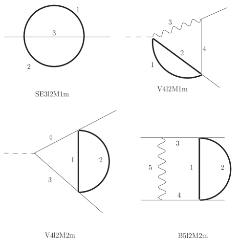
Figure 1: The topologies of the eight master integrals for the heavy-fermion corrections. Bold lines represent heavy fermions.

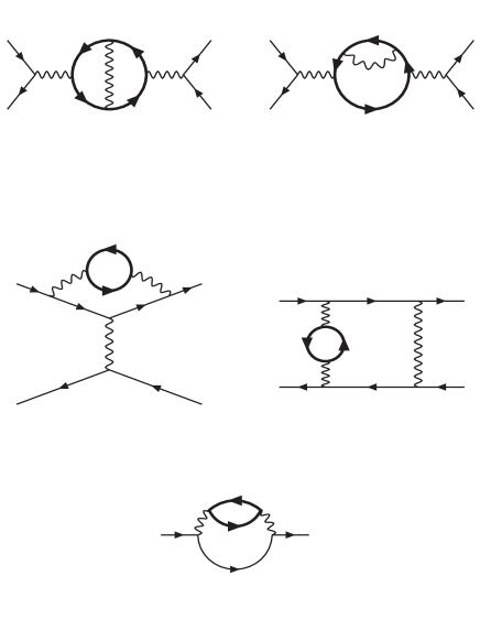
Figure 2: The diagrams for Bhabha scattering with two fermion flavors. Internal fermionic loops represent heavy leptons and the other fermion lines are electrons.

2 The planar two-loop boxes for $N_{f}=1$

There are 24 planar two-loop box MIs to be determined for the $N_{f}=1$ case, see Table 1. So far, we could not determine all of them analytically with the exact mass dependence; the status is reviewed in [31]. For this reason, we decided to treat these MIs uniquely in the approximation of small $m$ at fixed scattering angle. The results have been published in the mean time [23], so we will make here only few introductory remarks and show one example. In the list of MIs, we preferred to include Feynman integrals without any numerators. The pragmatic reason was the independence of their defintion on the internal flow of momenta. It is sufficient to indicate the lines with dots. Performing explicit calculations, one is, of course, faced with the observation that the singularities of dotted MIs and those with numerators are quite different. Evaluating the small mass expansions, we preferred in some cases to treat instead of dotted integrals those with numerators. Due to unique algebraic relations between all the integrals, there is no principal difference in these two approaches, and further details are discussed in [23]. Another observation concerns the MB-representations. In principle, one may use the representations for the basic 7-line boxes as given e.g. in [32] and shrink lines. However, when calculating MIs with numerators, additional representations have to be determined. We observed further, that it is sometimes not evident how to get an effective represenation for dotted MIs from more general ones. For the MI B5l2m2 (a 5-liner) we got, by shrinking of lines in B7l4m1 (first planar double box)and after expanding in $\varepsilon$, 11 MB-integrals with at most 4 integrations. From our direct derivation, we got 4 integrals, at most 3-dimensional. For the related dotted MI B5l2m2d2, we got from line shrinking 102 integrals, and by direct derivation only one, again 3-dimensional.

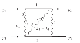
Figure 3: The 5-line topology B5l2m3. The momentum distribution has been chosen to make the derivation of the MB representation easier.

As an example, we reproduce here for the MI B5l2m3($k_{2}p_{3}$), shown in Figure 3, the basic $d$-dimensional MB-represenation:

$${\tt B5l2m3(p_{e}\cdot k_{2})}$$

$$=\frac{(-1)^{a_{12345}}\;e^{2\varepsilon\gamma_{E}}}{\prod_{j=1}^{5}\Gamma[a_{i}]\Gamma[4-2\varepsilon-a_{123}](2\pi i)^{4}}$$

$$\int_{-i\infty}^{+i\infty}d\alpha\int_{-i\infty}^{+i\infty}d\beta\int_{-i\infty}^{+i\infty}d\gamma\int_{-i\infty}^{+i\infty}d\delta$$

$$(-s)^{\gamma}\;(-t)^{(4-2\epsilon-a_{12345}-\beta-\delta-\gamma)}$$

$$\Gamma[-\beta]\;\Gamma[-\gamma]\;\Gamma[-\delta]\;\Gamma[a_{3}+\alpha+2\;\beta]\;$$

$$\frac{\Gamma[2-\epsilon-a_{45}+\alpha-\delta-\gamma]}{\Gamma[7-3\epsilon-a_{12345}-\beta]}$$

$$\frac{\Gamma[2-\epsilon-a_{13}-\beta]\;\Gamma[2-\epsilon-a_{23}-\alpha-\beta]}{\Gamma[a_{5}-\alpha+2\;\gamma]\;\Gamma[1+a_{5}-\alpha+2\;\gamma]}$$

$$\Gamma[-4+2\;\epsilon+a_{12345}+\beta+\delta+\gamma]$$

$$\biggl{\{}\Gamma[4-2\;\epsilon-a_{1235}-\beta-\delta-\gamma]$$

$$\biggl{[}(p_{e}\cdot p_{2})\;\Gamma[1+a_{5}+\gamma]\;\Gamma[-\alpha+\gamma]$$

$$-(p_{e}\cdot p_{1})\;\Gamma[a_{5}+\gamma]\;\Gamma[1-\alpha+\gamma]\biggr{]}$$

$$\Gamma[a_{5}-\alpha+2\;\gamma]\;\Gamma[1+a_{5}-\alpha+2\;\delta+2\;\gamma]$$

$$+[(p_{e}\cdot p_{3})-(p_{e}\cdot p_{1})]\;$$

$$\Gamma[5-2\epsilon-a_{1235}-\beta-\delta-\gamma]$$

$$\Gamma[a_{5}+\gamma]\;\Gamma[-\alpha+\gamma]\;\Gamma[1+a_{5}-\alpha+2\;\gamma]\;$$

$$\Gamma[a_{5}-\alpha+2\;(\delta+\gamma)]\biggr{\}}$$

The small mass expansion of the result is:

$${\tt B5l2m3(k_{2}\cdot p_{2})}=\frac{1}{4}\left(\frac{s}{u}\right)^{2}\biggl{\{}{\rm L}^{2}\;(6\;x\;\zeta_{2}$$

$$+2\;x\;\ln(x)+2\;x^{2}\;\ln(x)+x\;\ln^{2}(x))$$

$$+{\rm L}\;(16\;x\;\zeta_{2}-8\;x^{2}\;\zeta_{2}$$

$$-4\;x\;\zeta_{3}-2\;\ln(x)+2\;x^{2}\;\ln(x)$$

$$+4\;x\;\zeta_{2}\;\ln(x)+2\;x\;\ln^{2}(x)-2\;x^{2}\;\ln^{2}(x)$$

$$-12\;x\;\zeta_{2}\;\ln(1+x)$$

$$-2\;x\;\ln^{2}(x)\;\ln(1+x)-4\;x\;\ln(x)\;{{\rm{Li_{2}}}}(-x)$$

$$+4\;x\;{{\rm{Li_{3}}}}(-x))\biggr{\}}$$

$$+\frac{1}{120}\left(\frac{s}{u}\right)^{2}\biggl{\{}+120\;\zeta_{2}$$

$$+360\;x\;\zeta_{2}$$

$$-120\;x^{2}\;\zeta_{2}-1560\;x\;\zeta_{4}-480\;x\;\zeta_{3}$$

$$-240\;x^{2}\;\zeta_{3}-240\;x\;\zeta_{2}\;\ln(x)$$

$$-480\;x^{2}\;\zeta_{2}\;\ln(x)-360\;x\;\zeta_{3}\;\ln(x)$$

$$+30\;\ln^{2}(x)+60\;x\;\ln^{2}(x)-30\;x^{2}\;\ln^{2}(x)$$

$$-180\;x\;\zeta_{2}\;\ln^{2}(x)$$

$$-20\;x\;\ln^{3}(x)-20\;x^{2}\;\ln^{3}(x)-5\;x\;\ln^{4}(x)$$

$$+720\;x^{2}\;\zeta_{2}\;\ln(1+x)$$

$$+120\;x\;\zeta_{3}\;\ln(1+x)$$

$$-120\;x\;\zeta_{2}\;\ln(x)\;\ln(1+x)$$

$$+120\;x^{2}\;\ln^{2}(x)\;\ln(1+x)$$

$$+180\;x\;\zeta_{2}\;\ln^{2}(1+x)$$

$$+30\;x\;\ln^{2}(x)\;\ln^{2}(1+x)$$

$$+120\;x\;\ln(x)\;{\rm{S_{1,2}}}(-x)$$

$$+60\;x\;(-8\;\zeta_{2}-\ln^{2}(x)+2\;\ln(x)\;$$

$$(2\;x+\ln(1+x)))\;{{\rm{Li_{2}}}}(-x)$$

$$-240\;x^{2}\;{{\rm{Li_{3}}}}(-x)+240\;x\;\ln(x)\;{{\rm{Li_{3}}}}(-x)$$

$$-120\;x\;\ln(1+x)\;{{\rm{Li_{3}}}}(-x)$$

$$-360\;x\;{{\rm{Li_{4}}}}(-x)-120\;x\;{{\rm{S_{2,2}}}}(-x)\biggr{\}}$$

The expression is more complicated than those for the planar 7-line MIs concerning both the functions appearing as well as the dependence on all three Mandelstam variables $s,t,u$; the latter is typical for non-planar diagrams, where the B5l2m3 topology contributes.

3 The master integrals for the $N_{f}>1$ corrections

The differential Bhabha-scattering cross section with respect to the solid angle $\Omega$ can be written by means of an expansion in the fine-structure constant $\alpha$,

$$\frac{d\sigma}{d\Omega}=\frac{d\sigma_{0}}{d\Omega}+\left(\frac{\alpha}{\pi}\right)\frac{d\sigma_{1}}{d\Omega}+\left(\frac{\alpha}{\pi}\right)^{2}\frac{d\sigma_{2}}{d\Omega}+\ldots,$$ (1)

where $\sigma_{0}$ is the Born contribution and $\sigma_{i}$ ($i=1,2,\ldots$) represent the higher-order radiative corrections. If we are interested in the NNLO virtual contributions, we need to evaluate the diagrams of Figure 2, where the fermion self-energy is required for wave-function renormalization. Note that results for the photonic vacuum polarization diagrams can be found in [33].

After interfering the two-loop amplitude with the tree-level one, summing over the spins of the final state and averaging over those of the initial state, we get a large number of integrals. We use the DiaGen/IdSolver [34] implementation of the Laporta-Remiddi algorithm [10] in order to reduce all the needed Feynman integrals to a limited set of MIs. Apart from products of one-loop integrals, we get the eight MIs of Figure 1, as already pointed out in [13]. The corresponding Feynman integrals with $n$ propagators $D_{i}$ are defined as follows:

$$D(\{\nu_{i}\}_{n})=-\frac{(e^{\gamma})^{2\varepsilon}}{\pi^{d}}\int\frac{d^{d}k_{1}d^{d}k_{2}}{\prod_{i}^{n}D_{i}^{\nu_{i}}},$$ (2)

where $\gamma$ is the Euler-Mascheroni constant and we introduced the shorthand notations

$$\{\nu\}_{n} \equiv \nu_{1},\ldots,\nu_{n},$$

$$\nu_{ab\ldots c} \equiv \nu_{a}+\nu_{b}+\ldots+\nu_{c}.$$ (3)

In contrast to [23], we do not consider MIs with scalar products in the numerators. We have then to allow for higher powers of propagators. Of course, there are algebraic relations between MIs with scalar products in the numerators and MIs with propagators raised to higher powers.

We construct our MB representations using the standard approach described in [32]. The Feynman-parameter integrals are derived one after the other for the two subloops. In each step we replace the sum over monomials in the Feynman parameters by an appropriate MB representation. Due to the relatively simple structure of the considered diagrams, it is easier to begin with the propagator-type subloop.

As far as the electron self-energy is concerned, we only need the sunrise topology with the electron on its mass shell, $p_{1}^{2}=m^{2}$. A number of results for this mass configuration of the sunrise diagram can be found in the literature. Analytic expressions for the residues of the poles in dimensional regularization and the finite parts were given already in [35]. The explicit result for the ${\cal O}(\epsilon)$ terms, where $\epsilon\equiv(4-d)/2$ and $d$ are the space-time dimensions, can be found in [36]. Note that the inclusion of the ${\cal O}(\epsilon)$ terms for the sunrise MIs is mandatory when deriving the complete squared amplitude, since the reduction to MIs generates inverse powers of $\epsilon$.

For the self energy, we use our MB representation in order to reproduce the known result for the MIs. Its general form, for arbitrary powers $\nu_{i}$ of the propagators, is given by

$$\texttt{SE3l2M1m}(\{\nu\}_{3})=(m^{2})^{4-\nu_{123}-2\epsilon}$$ (4)

$$\times\frac{(-1)^{\nu_{123}}e^{2\gamma\epsilon}}{\prod_{i=1}^{3}\Gamma({\nu_{i}})}\int\frac{dz}{2\pi i}\left(\frac{m^{2}}{M^{2}}\right)^{z+\nu_{12}-2+\epsilon}$$

$$\times\frac{\prod_{i=1}^{6}\Gamma_{i}}{\Gamma(2z+\nu_{12})\Gamma(z-\nu_{3}+4-2\epsilon)}.$$

Furthermore, we defined

$$\Gamma_{1} \equiv\Gamma(-z),$$

$$\Gamma_{2} \equiv\Gamma(z+\nu_{1}),$$

$$\Gamma_{3} \equiv\Gamma(z+\nu_{2}),$$

$$\Gamma_{4} \equiv\Gamma(-z+\nu_{3}-2+\epsilon),$$

$$\Gamma_{5} \equiv\Gamma(2z-\nu_{3}+4-2\epsilon),$$

$$\Gamma_{6} \equiv\Gamma(z+\nu_{12}-2+\epsilon).$$ (5)

The integration contour is a straight line parallel to the imaginary axis separating the poles generated by $\Gamma_{1}$ and $\Gamma_{4}$ from those coming from $\Gamma_{2}$, $\Gamma_{3}$, $\Gamma_{5}$ and $\Gamma_{6}$.

The two sunrise MIs are defined by the following values for the powers of the propagators,

SE3l2M1m $$\equiv \texttt{SE3l2M1m}(1,1,1),$$

SE3l2M1md $$\equiv \texttt{SE3l2M1m}(1,2,1).$$ (6)

Having a MB representation at hand, one needs to perform an analytic continuation in $\varepsilon$ from a range where the integral is regular to the vicinity of the origin, uncovering the singular structure on the way. This is done by an automatized procedure implemented in the Mathematica package MB.m [37]. The resulting MB representations are verified numerically in the Euclidean region against the sector decomposition approach as described in [38].

For the sunrise MIs, a straightforward application of the Cauchy theorem to the MB representation of Eq. (4) leads to a sum over residua which can be easily evaluated. Therefore, we reproduced the results of [36]. In general, however, one has to deal with multiple MB representations. For the vertex and box MIs, the evaluation of the needed sums is far from being trivial.

As explained in the introduction, our purpose is to calculate the integrals by assuming a hierarchy of all scales, namely $m^{2}\ll M^{2}\ll s,t$. First of all we identify the leading contributions in the electron mass following the procedure described in [23]. Then, by using the Cauchy theorem to express the integrals through sums over residua, we evaluate these sums with the aid of XSUMMER [39].

For the sunrise MIs the results depend on one variable, $R\equiv m^{2}/M^{2}$, and read as

SE3l2M1m $$= \ M^{2}\ (m^{2})^{-2\epsilon}$$

$$\times\Bigl{[}\sum_{k=-2}^{1}\ S_{k}\ \epsilon^{k}\ +\ {\cal O}(\epsilon^{2})\Bigr{]},$$

$$S_{-2} = 1,$$ (7)

$$S_{-1} = 3+2\ln\left(R\right),$$

$$S_{0} = 7+\zeta_{2}+6\ln\left(R\right)+2\ln^{2}\left(R\right),$$

$$S_{1} = 15+3\zeta_{2}-\frac{2}{3}\zeta_{3}+\left(14+2\zeta_{2}\right)$$

$$\times\ln\left(R\right)+6\ln^{2}\left(R\right)+\frac{4}{3}\ln^{3}\left(R\right),$$

SE3l2M1md $$= (m^{2})^{-2\epsilon}\Bigl{[}\sum_{k=-2}^{1}S^{d}_{k}\epsilon^{k}+{\cal O}(\epsilon^{2})\Bigr{]},$$

$$S_{-2}^{d} = \frac{1}{2},$$ (8)

$$S^{d}_{-1} = \frac{1}{2}\Bigl{[}1+2\ln\left(R\right)\Bigr{]},$$

$$S_{0}^{d} = \frac{1}{2}\left(1+\zeta_{2}\right)+\ln\left(R\right)+\ln^{2}\left(R\right),$$

$$S_{1}^{d} = \frac{1}{6}\left(3+3\zeta_{2}-2\zeta_{3}\right)+\left(1+\zeta_{2}\right)$$

$$\times\ln\left(R\right)+\ln^{2}\left(R\right)+\frac{2}{3}\ln^{3}\left(R\right).$$

For vertices, the external electrons are on their mass shell, $p_{i}^{2}=m^{2}$, $i=1,2$, and we introduce the Mandelstam invariant $s\equiv(p_{1}+p_{2})^{2}$ (see Figure 1). Since each of the two vertices is related to two MIs, we have to consider

V4l2M1m $$\equiv \texttt{V4l2M1m}(1,1,1,1),$$

V4l2M1md $$\equiv \texttt{V4l2M1m}(1,1,1,2),$$

V4l2M2m $$\equiv \texttt{V4l2M2m}(1,1,1,1),$$

V4l2M2md $$\equiv \texttt{V4l2M2m}(1,2,1,1).$$ (9)

We follow the same strategy employed for the sunrise diagrams. First of all we derive the exact multi-dimensional MB representation, and then we perform first a small-mass expansions in $m_{s}$, and then in $M_{s}$, defined as the ratios of the fermion masses and the centre-of-mass energy, $m_{s}\equiv-m^{2}/s$, $M_{s}\equiv-M^{2}/s$. The MB representations read as

$$\texttt{V4l2M1m}(\{\nu\}_{4})=(m^{2})^{4-\nu_{1234}-2\epsilon}\\ \times\frac{(-1)^{\nu_{1234}}e^{2\gamma\epsilon}}{\prod_{i=1}^{4}\Gamma({\nu_{i}})}\int\frac{dz_{1}dz_{2}}{(2\pi i)^{2}}\\ \times m_{s}^{z_{2}-4+\nu_{1234}+2\epsilon}\,M_{s}^{-z_{1}+2-\nu_{12}-\epsilon}\\ \times\frac{\prod_{i=1}^{8}\Gamma_{i}}{\Gamma(2z_{1}+\nu_{12})\Gamma(z_{1}-\nu_{34}+4-2\epsilon)},\qquad$$ (10)

with

$$\Gamma_{1} \equiv\Gamma(z_{1}+\nu_{1}),$$

$$\Gamma_{2} \equiv\Gamma(z_{1}+\nu_{2}),$$

$$\Gamma_{3} \equiv\Gamma(z_{1}+\nu_{12}-2+\epsilon),$$

$$\Gamma_{4} \equiv\Gamma(-z_{2}),$$

$$\Gamma_{5} \equiv\Gamma(2z_{2}+\nu_{4}),$$

$$\Gamma_{6} \equiv\Gamma(-z_{2}-\nu_{34}+2-\epsilon),$$

$$\Gamma_{7} \equiv\Gamma(z_{1}-z_{2}-\nu_{4}+2-\epsilon),$$

$$\Gamma_{8} \equiv\Gamma(-z_{1}+z_{2}+\nu_{34}-2+\epsilon),$$ (11)

and

$$\texttt{V4l2M2m}(\{\nu\}_{4})=(m^{2})^{4-\nu_{1234}-2\epsilon}\\ \times\frac{(-1)^{\nu_{1234}}e^{2\gamma\epsilon}}{\prod_{i=1}^{4}\Gamma({\nu_{i}})}\int\frac{dz_{1}dz_{2}}{(2\pi i)^{2}}\\ \times m_{s}^{z_{2}-4+\nu_{1234}+2\epsilon}\,M_{s}^{-z_{1}+2-\nu_{12}-\epsilon}\\ \times\frac{\prod_{i=1}^{9}\Gamma_{i}}{\prod_{j=10}^{12}\Gamma_{j}},\qquad\qquad\qquad\qquad\qquad\qquad$$ (12)

with

$$\Gamma_{1} \equiv\Gamma(-z_{1}),$$

$$\Gamma_{2} \equiv\Gamma(z_{1}+\nu_{1}),$$

$$\Gamma_{3} \equiv\Gamma(z_{1}+\nu_{2}),$$

$$\Gamma_{4} \equiv\Gamma(z_{1}+\nu_{12}-2+\epsilon),$$

$$\Gamma_{5} \equiv\Gamma(2z_{1}-\nu_{34}+4-2\epsilon),$$

$$\Gamma_{6} \equiv\Gamma(-z_{2}),$$

$$\Gamma_{7} \equiv\Gamma(z_{1}-z_{2}-\nu_{3}+2-\epsilon),$$

$$\Gamma_{8} \equiv\Gamma(z_{1}-z_{2}-\nu_{4}+2-\epsilon),$$

$$\Gamma_{9} \equiv\Gamma(-z_{1}+z_{2}+\nu_{34}-2+\epsilon),$$

$$\Gamma_{10} \equiv\Gamma(2z_{1}+\nu_{12}),$$

$$\Gamma_{11} \equiv\Gamma(z_{1}-\nu_{34}+4-2\epsilon),$$

$$\Gamma_{12} \equiv\Gamma(2z_{1}-2z_{2}-\nu_{34}+4-2\epsilon).$$ (13)

A careful analysis of the powers of $m_{s}$ and $M_{s}$ under the MB integrals leads to the following results,

V4l2M1m $$= (m^{2})^{-2\epsilon}\Bigl{[}\sum_{k=-2}^{0}V^{1}_{k}\epsilon^{k}+{\cal O}(\epsilon)\Bigr{]},$$

$$V^{1}_{-2} = \frac{1}{2},$$

$$V^{1}_{-1} = \frac{5}{2},$$ (14)

$$V^{1}_{0} = \frac{1}{2}\left[19-3\zeta_{2}-\ln^{2}(m_{s})\right],$$

V4l2M1md $$= \frac{(m^{2})^{-2\epsilon}}{m^{2}}\Bigl{[}\sum_{k=-2}^{0}V^{1d}_{k}\epsilon^{k}+{\cal O}(\epsilon)\Bigr{]},$$

$$V^{1d}_{-2} = \frac{1}{2},$$

$$V^{1d}_{-1} = 1+\frac{1}{2}\ln(m_{s}),$$ (15)

$$V^{1d}_{0} = 2-\zeta_{2}+\ln(m_{s})+\frac{1}{4}\ln^{2}(m_{s}),$$

V4l2M2m $$= (m^{2})^{-2\epsilon}\Bigl{[}\sum_{k=-2}^{0}V^{2}_{k}\epsilon^{k}+{\cal O}(\epsilon)\Bigr{]},$$

$$V^{2}_{-2} = \frac{1}{2},$$

$$V^{2}_{-1} = \frac{5}{2}+\ln(m_{s}),$$

$$V^{2}_{0} = \frac{1}{2}(19+\zeta_{2})+5\ln(m_{s})$$ (16)

$$+ \ln^{2}(m_{s}),$$

V4l2M2md $$= (m^{2})^{-2\epsilon}\frac{1}{s}\Bigl{[}V^{2d}_{0}+{\cal O}(\epsilon)\Bigr{]},$$

$$V^{2d}_{0} = \frac{1}{6}\Bigl{[}12\zeta_{3}-6\zeta_{2}\ln(M_{s})$$ (17)

$$- \ln^{3}(M_{s})\Bigr{]}.$$

For box diagrams, the external momenta are again on their mass shell, and we have additionally $(p_{1}-p_{3})^{2}=t$. After introducing $M_{t}\equiv-M^{2}/t$, the appropriate MB representation is given by

$$\texttt{B5l2M2m}(\{\nu\}_{5})=(m^{2})^{4-\nu_{12345}-2\epsilon}\\ \times\frac{(-1)^{\nu_{12345}}e^{2\gamma\epsilon}}{\prod_{i=1}^{5}\Gamma({\nu_{i}})}\int\frac{dz_{1}dz_{2}dz_{3}}{(2\pi i)^{3}}\\ \times M_{t}^{-z_{1}+2-\nu_{12}-\epsilon}m_{s}^{z_{3}-4+\nu_{12345}+2\epsilon}\\ \times\left(\frac{t}{s}\right)^{z_{2}-z_{1}+2-\nu_{12}-\epsilon}\frac{\prod_{i=1}^{11}\Gamma_{i}}{\prod_{j=12}^{14}\Gamma_{j}},\qquad$$ (18)

with

$$\Gamma_{1} \equiv\Gamma(z_{1}+\nu_{1}),$$ (19)

$$\Gamma_{2} \equiv\Gamma(z_{1}+\nu_{2}),$$

$$\Gamma_{3} \equiv\Gamma(z_{1}+\nu_{12}-2+\epsilon),$$

$$\Gamma_{4} \equiv\Gamma(-z_{2}),$$

$$\Gamma_{5} \equiv\Gamma(z_{2}+\nu_{4}),$$

$$\Gamma_{6} \equiv\Gamma(-z_{3}),$$

$$\Gamma_{7} \equiv\Gamma(-z_{1}+z_{2}),$$

$$\Gamma_{8} \equiv\Gamma(2z_{1}\!-\!2z_{2}-\nu_{3445}+4-2\epsilon),$$

$$\Gamma_{9} \equiv\Gamma(z_{1}-z_{2}-z_{3}-\nu_{34}+2-\epsilon),$$

$$\Gamma_{10} \equiv\Gamma(z_{1}\!-\!z_{2}\!-\!z_{3}-\nu_{45}+2-\epsilon),$$

$$\Gamma_{11} \equiv\Gamma(-z_{1}+z_{2}+z_{3}+\nu_{345}-2+\epsilon),$$

$$\Gamma_{12} \equiv\Gamma(2z_{1}+\nu_{12}),$$

$$\Gamma_{13} \equiv\Gamma(z_{1}-\nu_{345}+4-2\epsilon),$$

$$\Gamma_{14} \equiv\Gamma(2(z_{1}\!-\!z_{2}\!-\!z_{3})-\nu_{3445}+4-2\epsilon).$$

We have to compute two MIs,

B5l2M2m $$\equiv \texttt{B5l2M2m}(1,1,1,1,1),$$

B5l2M2md $$\equiv \texttt{B5l2M2m}(1,2,1,1,1),$$ (20)

and an expansion in the high-energy limit of the appropriate three-fold MB representations leads to the following results,

B5l2M2m $$= (m^{2})^{-2\epsilon}\Bigl{[}\sum_{k=-2}^{0}B_{k}\epsilon^{k}+{\cal O}(\epsilon)\Bigr{]},$$

$$B_{-2} = \frac{1}{s}\ln(m_{s}),$$

$$B_{-1} = \frac{1}{s}\Bigl{(}-\zeta_{2}+2\ln(m_{s})+\frac{1}{2}\ln^{2}(m_{s})$$

$$+ \ln(m_{s})\ln(m_{t})\Bigr{)},$$

$$B_{0} = \frac{1}{s}\Bigl{[}-2\zeta_{2}-2\zeta_{3}+4\ln(m_{s})+\ln^{2}(m_{s})$$ (21)

$$+ \frac{1}{3}\ln^{3}(m_{s})-4\zeta_{2}\ln(m_{t})$$

$$+ 2\ln(m_{s})\ln(m_{t})+\ln(m_{s})\ln^{2}(m_{t})$$

$$- \frac{1}{6}\ln^{3}(m_{t})$$

$$- \Bigl{(}3\zeta_{2}+\frac{1}{2}\ln^{2}(m_{s})-\ln(m_{s})\ln(m_{t})$$

$$+ \frac{1}{2}\ln^{2}(m_{t})\Bigr{)}\ln\left(1+\frac{t}{s}\right)$$

$$- \Bigl{(}\ln(m_{s})-\ln(m_{t})\Bigr{)}\text{Li}_{2}\left(-\frac{t}{s}\right)$$

$$+ \text{Li}_{3}\left(-\frac{t}{s}\right)\Bigr{]},$$

B5l2M2md $$= (m^{2})^{-2\epsilon}\Bigl{[}\sum_{k=-1}^{0}B^{d}_{k}\epsilon^{k}+{\cal O}(\epsilon)\Bigr{]},$$

$$B^{d}_{-1} = -\frac{1}{st}\Bigl{[}\ln(m_{s})\ln(m_{t})-\ln(m_{s})L(R)\Bigr{]},$$

$$B^{d}_{0} = \frac{1}{st}\Bigl{\{}-2\zeta_{3}+\zeta_{2}\ln(m_{s})+4\zeta_{2}\ln(m_{t})$$

$$- 2\ln(m_{s})\ln^{2}(m_{t})+\frac{1}{6}\ln^{3}(m_{t})$$

$$- 2\zeta_{2}L(R)+2\ln(m_{s})\ln(m_{t})L(R)$$

$$- \frac{1}{6}L^{3}(R)$$

$$+ \Bigl{(}3\zeta_{2}+\frac{1}{2}\ln^{2}(m_{s})-\ln(m_{s})\ln(m_{t})$$

$$+ \frac{1}{2}\ln^{2}(m_{t})\Bigr{)}\ln\left(1+\frac{t}{s}\right)$$

$$+ \Bigl{(}\ln(m_{s})-\ln(m_{t})\Bigr{)}\text{Li}_{2}\left(-\frac{t}{s}\right)$$

$$- \text{Li}_{3}\left(-\frac{t}{s}\right)\Bigr{\}}.$$

4 Summation techniques

In any realistic computation we have to check the structure of the ultraviolet (UV) and infrared (IR) divergencies. By combining the Mellin-Barnes method with recently developed summation techniques we are able to evaluate exactly (i.e. without a high-energy approximation) the residues of the UV and IR poles for each MI.

A simple example is enough to illustrate our procedure. We consider the following one-fold integral in the complex plane, related to the single pole of V4l2M1md,

$$I\equiv\frac{1}{2\pi i}\int_{c-i\infty}^{c+i\infty}dz\ M_{s}^{-z}\ \frac{\prod_{i=1}^{3}\Gamma_{i}}{\Gamma(2z+2)},$$ (23)

where we recall that $M_{s}\equiv-M^{2}/s$, the integration contour is a straight line parallel to the imaginary axis, $c=-1/2$ and we introduced

$$\Gamma_{1} \equiv\Gamma(-z),$$

$$\Gamma_{2} \equiv\Gamma(z),$$

$$\Gamma_{3} \equiv\Gamma^{2}(z+1).$$ (24)

After closing the integration contour to the right of the complex plane and taking residua, the integral $I$ can be written by means of two inverse binomial sums,

$$I = \sum_{n=1}^{\infty}\left(-1\right)^{n}\ M_{s}^{-n}\frac{1}{\binom{2n}{n}}\left(\frac{1}{n}-\frac{2}{2n+1}\right)$$ (25)

$$- 2-\ln\left(M_{s}\right).$$

Inverse binomial sums were recently studied by means of the log-sine approach in [40]. Another approach was developed in [41] by generalizing the summation algorithms introduced in [42]. A straightforward application of these techniques leads to a compact result,

$$I=\frac{1-x_{M}}{1+x_{M}}\ln(y_{M})\left(1+4M_{s}\right)-\ln\left(M_{s}\right),$$ (26)

where we introduced the variables $x_{M}$ and $y_{M}$,

$$x_{M} \equiv \frac{\sqrt{4M^{2}-s}-\sqrt{-s}}{\sqrt{4M^{2}-s}+\sqrt{-s}},$$

$$y_{M} \equiv \frac{\sqrt{4M^{2}-t}-\sqrt{-t}}{\sqrt{4M^{2}-t}+\sqrt{-t}}.$$ (27)

As an example, after additionally introducing the following variables,

$$x_{m} \equiv \frac{\sqrt{4m^{2}-s}-\sqrt{-s}}{\sqrt{4m^{2}-s}+\sqrt{-s}},$$

$$y_{m} \equiv \frac{\sqrt{4m^{2}-t}-\sqrt{-t}}{\sqrt{4m^{2}-t}+\sqrt{-t}},$$ (28)

we get the non-approximated expressions for the residues of the poles of the two box diagrams defined in Eq. (3),

$$B_{-2} = -\frac{1}{m^{2}}\frac{x_{m}}{1-x_{m}^{2}}H(0;x_{m}),$$

$$B_{-1} = \frac{1}{2m^{2}}\frac{x_{m}}{1-x_{m}^{2}}\Bigl{\{}-H^{2}(0;x_{m})$$ (29)

$$+ 2\Bigl{[}\zeta_{2}-2H(0,-1;x_{m})\Bigr{]}$$

$$+ 2H(0;x_{m})\Bigl{[}2H(-1;x_{m})$$

$$- \frac{1+y_{M}}{1-y_{M}}H(0;y_{M})-2$$

$$- \ln\left(\frac{m^{2}}{M^{2}}\right)\Bigr{]}\Bigr{\}},$$

and

$$B^{d}_{-1} = -\frac{1}{m^{2}M^{2}}\frac{x_{m}\,y_{M}}{(1-x_{m}^{2})(1-y_{M}^{2})}$$ (30)

$$\times H(0;x_{m})H(0;y_{M}),$$

where we used the HPLs introduced in [15].

For completeness, we add here also the exact expressions for the diveregent parts of the vertex MIs:

$$V^{1d}_{-1} = \frac{1}{2}\left\{\frac{1+x_{M}}{1-x_{M}}H(0;x_{M})+2+\ln R\right\}$$

$$V^{2}_{-1} = \frac{5}{2}+\frac{1+x_{m}}{1-x_{m}}H(0;x_{m}).$$ (31)

5 Summary

From [13] we know the table of MIs for massive two-loop Bhabha scattering. We were able to express all the Feynman integrals occurring in the amplitude through these MIs by algebraic relations. We presented at the workshop all the planar two-loop box MIs. The $N_{f}=1$ MIs has been published in the meantime [23]. In this contribution, we provide the expanded results for all the MIs entering the Bhabha-scattering amplitude with two fermion flavors in the limit of small fermion masses at fixed scattering angle. The MIs may be also found at our webpage [43]. These MIs were one of the last missing ingredients for the evaluation of the virtual two-loop contribution to the differential cross-section.

The computation of the last nine non-planar two-loop box MIs is under way.

References

[1]
M. Consoli,
Nucl. Phys. B160 (1979) 208.
[2]
Z. Bern, L. Dixon and A. Ghinculov,
Phys. Rev. D63 (2001) 053007, hep-ph/0010075.
[3]
A.B. Arbuzov et al.,
Nucl. Phys. B474 (1996) 271.
[5]
A. Arbuzov, E. Kuraev and B.G. Shaikhatdenov,
Mod. Phys. Lett. A13 (1998) 2305, hep-ph/9806215.
[6]
N. Glover, B. Tausk and J. van der Bij,
Phys. Lett. B516 (2001) 33, hep-ph/0106052.
[7]
A. Penin,
Phys. Rev. Lett. 95 (2005) 010408, hep-ph/0501120.
[8]
A. Penin,
Nucl. Phys. B734 (2006) 185, hep-ph/0508127.
[9]
A. Penin,
Nucl. Phys. Proc. Suppl. 157 (2006) 6.
[10]
S. Laporta and E. Remiddi,
Phys. Lett. B379 (1996) 283, hep-ph/9602417.
[11]
S. Laporta,
Int. J. Mod. Phys. A15 (2000) 5087, hep-ph/0102033.
[12]
R. Bonciani et al.,
Nucl. Phys. B681 (2004) 261, hep-ph/0310333.
[13]
M. Czakon, J. Gluza and T. Riemann,
Phys. Rev. D71 (2005) 073009, hep-ph/0412164.
[14]
M. Czakon, J. Gluza and T. Riemann,
Acta Phys. Polon. B36 (2005) 3319, hep-ph/0511187.
[15]
E. Remiddi and J. Vermaseren,
Int. J. Mod. Phys. A15 (2000) 725, hep-ph/9905237.
[16]
M. Czakon, J. Gluza and T. Riemann,
Nucl. Instrum. Meth. A559 (2006) 265, hep-ph/0508212.
[17]
R. Bonciani et al.,
Nucl. Phys. B701 (2004) 121, hep-ph/0405275.
[18]
R. Bonciani et al.,
Nucl. Phys. B716 (2005) 280, hep-ph/0411321.
[19]
R. Bonciani and A. Ferroglia,
Phys. Rev. D72 (2005) 056004, hep-ph/0507047.
[20]
R. Bonciani and A. Ferroglia,
Nucl. Phys. Proc. Suppl. 157 (2006) 11, hep-ph/0601246.
[21]
J. Fleischer, J. Gluza, A. Lorca and T. Riemann,
First order radiative corrections to Bhabha scattering in dimensions, to appear in Eur. Phys. J. C,
hep-ph/0606210.
[22]
V. Smirnov,
Phys. Lett. B524 (2002) 129, hep-ph/0111160.
[23]
M. Czakon, J. Gluza and T. Riemann,
Nucl. Phys. B751 (2006) 1, hep-ph/0604101.
[24]
G. Heinrich and V. Smirnov,
Phys. Lett. B598 (2004) 55, hep-ph/0406053.
[25]
M. Czakon, J. Gluza and T. Riemann,
Nucl. Phys. (Proc. Suppl.) B135 (2004) 83, hep-ph/0406203.
[26]
N. Usyukina,
Teor. Mat. Fiz. 22 (1975) 300.
[27]
E. Boos and A. Davydychev,
Theor. Math. Phys. 89 (1991) 1052.
[28]
V. Smirnov,
Phys. Lett. B460 (1999) 397, hep-ph/9905323.
[29]
B. Tausk,
Phys. Lett. B469 (1999) 225, hep-ph/9909506.
[30]
B. Kniehl et al.,
Phys. Lett. B209 (1988) 337.
[31]
M. Czakon, J. Gluza, K. Kajda and T. Riemann,
Nucl. Phys. Proc. Suppl. 157 (2006) 16,
hep-ph/0602102.
[32]
V. Smirnov,
Evaluating Feynman Integrals, Springer Tracts in Modern Physics Vol.
211 (Springer, Berlin, 2004).
[33]
G. Kallen and A. Sabry,
Kong. Dan. Vid. Sel. Mat. Fys. Med. 29N17 (1955) 1.
[34]
M. Czakon,
DiaGen/IdSolver, unpublished.
[35]
F. Berends, A. Davydychev and N. Ussyukina,
Phys. Lett. B426 (1998) 95, hep-ph/9712209.
[36]
M. Argeri, P. Mastrolia and E. Remiddi,
Nucl. Phys. B631 (2002) 388, hep-ph/0202123.
[37]
M. Czakon,
Automatized analytic continuation of Mellin-Barnes integrals, to appear in Comput. Phys. Commun.,
hep-ph/0511200.
[38]
T. Binoth and G. Heinrich,
Nucl. Phys. B680 (2004) 375, hep-ph/0305234.
[39]
S. Moch and P. Uwer,
Comput. Phys. Commun. 174 (2006) 759, math-ph/0508008.
[40]
A. Davydychev and M. Kalmykov,
Nucl. Phys. B699 (2004) 3, hep-th/0303162.
[41]
S. Weinzierl,
J. Math. Phys. 45 (2004) 2656, hep-ph/0402131.
[42]
S. Moch, P. Uwer and S. Weinzierl,
J. Math. Phys. 43 (2002) 3363, hep-ph/0110083.
[43]
S. Actis, M. Czakon, J. Gluza and T. Riemann,
http://www-zeuthen.desy.de/theory/research/bhabha/.