About Mass, CP and Extra Dimensions

Abstract

We discuss the notion of mass, mostly for fermions, and its relation to the breaking of CP invariance, the natural symmetry of gauge interactions. In a first model, we show how compactification on a Vortex in 2 extra dimensions leads to a replication of generations in 3+1, with challenging mass patterns, and testable consequences in flavour-changing neutral currents (family-number conserving), both at low energies and at future colliders. In different model, we show how CP violation can result from compactification from 4+1 to 3+1 dimensions.

1 Introduction

While gauge boson masses are intimately linked to broken local symmetry, no such logical connection occurs in general for fermions. In the Standard Model, at least some of the mass must be linked to symmetry breaking, but this is due to the fact that left- and right-handed fermions are not in the same representations. Hypothetical vectorlike fermions could indeed have masses without symmetry breaking. Another situation is known for the effective, sometimes called ”constituant” mass. It is usually interpreted as a result of strong interactions leading to a breaking of chiral symmetry, and used as a model for ”dynamical symmetry breaking”. Quite another possible origin for masses is from extra dimensions. Here the problem is almost the opposite. If the scales associated with extra dimensions are heavy, it is now a matter of preserving some light states. This is often realized through some form of localisation on topological singularities: domain walls in one, or vortices for two extradimensions.

In this presentation, we review two topics relating fermion masses and extra dimensions. The first aspect may seem at first a variant of fermion ”multilocalisation”, overlaps leading to the generation of mass patterns from overlap of wave functions in extra dimensions. The scheme considered here is however much more constrained and deterministic, as the fermions are all localized in the same way on a unique topological singularity, and the overlap functions are precisely determined by the dynamics of this singularity. This work is based on the series of papers Frere:2000dc ,Frere:2001ug ,Frere:2003yv , Frere:2003ye ,with predictions for colliders in Frere:2004yu and recent conjectures about a light Brout-Englert-Higgs particle in Libanov:2005mv .

The second part deals with another fundamental question, namely: ”How does CP (or T) violation enter in a fundamental theory?”. The main point is that CP is the natural symmetry of gauge interactions, and therefore attempts at unifying scalar couplings (effective or not) with gauge interactions pose the problem of breaking CP symmetry. We prove that this can occur through dimensional reduction, by the inclusion of ”Hosotani loops” (in this case, the equivalent of Wilson loops, but looping around the extra dimension). In a simple example, we generate CP violation from a 4+1 theory with only real couplings. This work is based on reference Cosme:2002zv , and its generalization to include grand unified structures Cosme:2003cq .

2 Three Families in One

In this section, we describe in general terms a model evolved in collaboration with Serguey Troitsky and Maxim Libanov. Full mathematical details can be found in the original papers, and we will here mainly list the salient results.

It may still be useful to start with a little history of the model. It was initially introduced by S. Troitsky and M. Libanov in a different form, possibly lighter in field content, but with only approximate symmetry. Libanov:2000uf , using a vortex of winding number 3. The following version, still formulated for flat extra dimensions, simulated this vortex with a scalar field of winding number one (with cubic coupling to fermions, and avoided any explicit breaking of symmetry by introducing supplementary scalar fields.Frere:2000dc

In both cases, the first rationale for the use of a topological defect (the vortex) was to confine the fermions to a small region of the extra-dimensional space, taken otherwise to be flat and infinite. The vortex being built out of a scalar field $\Phi$ and an auxiliary gauge field $A^{\mu}$ (both unrelated to the Standard Model fields, these fields don’t enter directly the currently observable phenomenology), it is possible to apply the Index theorem, and to conclude that for an effective winding number $n$ exactly $n$ massless chiral fermion modes persist in the remaining 3+1 dimensions for each fermion field coupling to the 6-d structure.

We have thus developed the phenomenology from this onset, but soon realized that the flat and unbounded extra dimensions represented a liability, with the need of confining the observed gauge fields, which otherwise could couple to fermionic modes outside the structure. A more involved version, largely with the same characteristics, was thus developed with the extra dimensions now assuming spherical topology.

Why maintain the topological singularity?

Part of the answer lies of course in the counting of light (massless at compactification scale) fermion modes, and the resulting replication as an origin to the very notion of particle families.

Obviously, the number of light fermions is not a direct prediction of the model in its present state, as we have to put in by hand the winding number, but the mass hierarchy of fermions, and a number of phenomenological implications are quite generic. We will detail them somewhat now.

2.1 The Model - fermion wave functions and mass hierarchies

While the latest formulation has the extra dimensions on a sphere, we will for pedagogical reasons describe the situation for a plane. The outcome in terms of fermion wave functions, selection rules and masses is very similar. For the plane, the extra variables are chosen as $(r,\varphi)$, while for the sphere (of radius $R$) we use $(R\theta,\varphi)$. Assuming the above-mentioned vortex structure is described by a field $\Phi$ such that

$$\Phi(x,r,\varphi)=\Phi(x)\ {\Phi}_{1}(r)\ e^{i\varphi}$$ (1)

This of course has only winding number 1, but the winding number 3 structure is achieved by coupling all the fermion fields according to:

$$\overline{\Psi}\Phi^{3}\Psi$$ (2)

This coupling may look surprising, as it is obviously non-renormalisable in 4 dimensions. We are not considering renormalisability of the theory here, as the 6 dimensional context is most likely an effective model, but even in this case it might be suitable that the 4-dim reduction be renormalisable. In this context, the reason we proceed as above is mostly simplicity: we could obviously replace this structure with a winding-3 solution for a fundamental field $\widetilde{\Phi}$, and find similar solutions for the couplings which will follow. This would however unnecessarily clutter the discussion, and we opt at this point for the simplicity of the field content.

The Yukawa coupling in equation (2) is only responsible for linking the fermions to the vortex. For each type of fermion field $\Psi_{T}$ introduced. Here the type $T$ represents the various quarks, $U_{R},D_{R},Q_{L}=(U_{L},D_{L})$ or the leptons and the indices $L,R$ refer to the 4-dim chirality of the associated particles after dimensional reduction. Only one field is introduced to represent all the ”up” quarks, for instance. The vortex structure leads, through the index theorem to 3 massless localized chiral solutions in 3+1 dimensions, which we will associate with the family replication. Typically, we have

$${\Psi_{T}}_{n}\sim{f_{T}}_{n}(r)e^{i(3-n)\varphi}$$ (3)

What is important here is that each ”family” of solutions has a different ”winding” behaviour in the variable $\varphi$. The labeling of the modes is quite arbitrary; it was chosen here so that in the simplest case the larger mass is associated to the third generation. Rather than analytic expressions, we give a pictorial representation of the radial dependence of the corresponding functions ${f_{T}}_{n}(r)$.

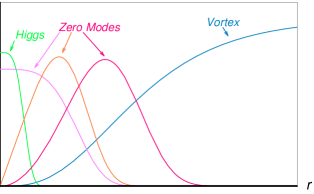
Figure 1: Profiles of the relevant wave functions in the radial coordinate

The fermionic mode 3 is non-vanishing at $r=0$ , with the modes behaving near the origin as:

$${f_{T}}_{n}(r)\sim r^{3-n}\ \;\ \ r\rightarrow 0$$ (4)

We have thus realized a situation similar to, but much more constrained than the multilocalisation in 5 dimensions. Here, we don’t have the freedom to place our various families at arbitrary spacing, but are faced instead with non-trivial overlaps fixed by the vortex properties.

This far, we only dealt with the ”background” of the problem, and generated essentially massless states in 3+1 dimensions. Now comes the time to generate the ”usual” fermion masses, and to break the $SU(3)XSU(2)XU(1)$ symmetry. This is done in the usual way, through the Brout-Englert-Higgs mechanism, at the price of introducing a scalar doublet, which we will name $H$. In fact, for the purpose of separating the various quantum numbers, we write, instead of the usual coupling:

$${\cal L}_{Yukawa}=\lambda_{U}\Psi_{U_{R}}H^{\dagger}X\Psi_{Q_{L}}+\epsilon\lambda_{U}\Psi_{U_{R}}\ H^{\dagger}\Phi\Psi_{Q_{L}}+h.c.$$ (5)

where $\Phi$ is the background field already described, while $X$ is a singlet with non-vanishing value at $r=0$ and winding number 0. The reason for introducing these couplings and $X$ itself, is to simplify the breaking structure; it would be perfectly possible to introduce single fields to replace the combinations $H\Phi$ and $HX$. Obviously, similar terms obtain for the other fermion types.

The $H$ field also couples to $\Phi$, and this results in a non-trivial profile, centered at the origin, and exemplified in figure1. Note that $H^{\dagger}X$ and $H^{\dagger}\varphi$

$$H^{\dagger}X \sim e^{i\ 0\ \varphi}$$ (6)

$$H^{\dagger}\varphi \sim e^{i\varphi}$$ (7)

2.2 Mixing of families and alternatives

The reduction to 4 dimensions involves integration over $\varphi$ and $r$ (or $\theta=r/R$ in the case of a sphere) and generates the mass terms (we just give the ”up” quark as an example,and neglect the term in $\epsilon$ for the time being):

$$m_{U,ij}=\lambda\int dr\int d\varphi f_{{U_{R}},i}^{\dagger}f_{{Q_{L}},j}\ X(r)\ H(r)e^{i(j-i)\varphi}$$ (8)

Clearly, the integration over $\varphi$ guarantees that only diagonal entries occur, and the ratio of the masses is given by the overlap between the fermion and scalar wave functions in the coordinate $r$. If, for instance, the profile of the scalar combination is concentrated close to the origin (as suggested in figure 1), we get $m_{3}>>m_{2}>>m_{1}$ (more on this later).

Mixing is however needed, and it can be introduced by the term proportional to $H^{\dagger}\Phi$ in equation (5). This results in a mass matrix

$$m_{U,ij}=\left(\begin{array}[]{ccc}m_{1}&\epsilon\ m_{12}&0\\ 0&m_{2}&\epsilon\ m_{23}\\ 0&0&m_{3}\\ \end{array}\right)$$ (9)

The mass eigenstates are obtained by diagonalization, but the Kobayashi-Maskawa matrix itself finds its origin in the differential rotation of the ”up” and ”down” quarks. That these rotations are different can result from different choices of $\lambda,\epsilon$.

The possibility also exists to use completely different patterns, for instance choosing the $H^{\dagger}\Phi$ contribution as leading (which we are free to do, since the Yukawa couplings are arbitrary) leads to a completely off-diagonal mass matrix, a feature which can come in handy when dealing with the large rotations between neutrinos and charged leptons.

2.3 Family number near-conservation and Kaluza-Klein modes; Experimental constraints

We turn now to the gauge interactions, and to their effect in 3+1 diemnsions. As usual, we will need to face a number of Kaluza-Klein excitations for each gauge boson introduced. In the present case, each such ”tower” carries a double label, since it must refer both to radial and angular excitations. Generically, ($A$ stands for any gauge boson, $\gamma$, W, Z, gluons):

$$A_{lm}(r,\varphi)=a_{lm}(r){\rm e}^{im\varphi}$$ (10)

The lowest state (massless before symmetry breaking) has a flat profile in both variables, which guarantees charge universality on one hand, and diagonal couplings (even in the mass basis) for the neutral bosons. Mass relations between the $lm$ modes depend on the topology of the model.

We will focus in this section on a particular feature of our approach, namely the presence of flavour-changing neutral currents, but with approximate conservation of ”family number”. Indeed, even if we neglect the Kobayashi-Maskawa mixing, the $m\neq 0$ modes generate transitions between families. Winding number ($\varphi$ dependence) acts as an effective ”family number”, which is conserved at both vertices where an excitation $A_{lm}$ connects to the fermions. For instance, the $Z$ boson excitations $Z^{\prime}\sim e^{\pm i\varphi}$, allow the following transitions:

$$s+\overline{d}\Rightarrow Z^{\prime}\Rightarrow s+\overline{d},$$ (11)

$$s+\overline{d}\Rightarrow Z^{\prime}\Rightarrow\mu+\overline{e},$$ (12)

$$s+\overline{d}\Rightarrow Z^{\prime}\Rightarrow\tau+\overline{\mu}$$ (13)

As discussed in Frere:2003ye , this leads to powefull constraints. In particular, the second process above induces the transition $K\Rightarrow\mu+\overline{e}$, which is severely constrained experimentally. The strength of the interaction is given by the usual gauge coupling constant, the mass of the $Z^{\prime}$ excitation, and an extra factor due to the overlap of the wave functions for fermions of the first and second generation, and the radial dependence of the $Z^{\prime}$: $\kappa_{1,2}=\int dr\ f_{{U_{R}},1}^{\dagger}\ f_{{Q_{L}},2}\ z_{0,1}(r)$, leading to the limit:

$$M_{Z^{\prime}}\geq\kappa_{12}\cdot 100{\rm TeV}$$ (14)

Future tests of this model will benefit much from currently planned precision lepton flavour violation experiments at moderate energies, as well as collider experiments trying to produce directly the Kaluza-Klein excitations.

2.4 Expectations at colliders

We expect mainly two types manifestations at colliders:

• the Brout-Englert-Higgs boson mass

• production of the Kaluza-Klein excitations.

The first issue is tackled in Libanov:2005mv , where a connection between the mass of $H$ and the extension of the scalar wave function in the extra coordinate $r$. As already specified, large mass ratios $m_{3}/m_{2},m_{2}/m_{1}$ require that the wave function be quite concentrated close to the origin. For the simplest scheme discussed above, Libanov:2005mv gets an upper bound close to the current limit.

The second issue deals with direct production of Kaluza-Klein excitations. As seen from equation (14), there is here a trade-off between the overlap factor and the actual mass of the new gauge boson. Constraints from K meson decays put the mass range above in the (unlikely) case that the overlap factor $\kappa$ is close to 1. This is clearly out of reach of LHC, but a smaller overlap may bring the scale down considerably, albeit at the cost of production efficiency (thus requiring the full luminosity for detection). We have studied this production as a function of $\kappa$, assuming the bound on $M$ to be saturated in each case; in Frere:2004yu , we see that for an integrated luminosity of $100fb^{-1}$ and $\sqrt{s}=14TeV$, a few events can be expected if $M<3TeV$ in the $\mu^{+}e^{-}$ final mode (the charge-conjugate channel is less sensitive). Note however that this is an exceptionally clean final state to look for!

Considerably more events are expected if we deal with the Kaluza-Klein excitations of the gluons instead, but there, even if the family-number near conservation still obtains, the extraction of the signal will be considerably more difficult, and detailed modeling is requested.

3 CP violation from extra dimensions

3.1 A toy model

The motivation for this work was given already in the introduction: if a fundamental theory has all couplings related to gauge interactions, how can it violate the natural symmetry of those, i.e., CP ? One possibility is to have spontaneous CP violation, involving several, relatively complex vacuum expectation values. This is certainly possible, requires at least 3 such vev’s, but can appear somewhat contrived. We look here for a more structural approach.

We start with a simple example, showing how a complex mass matrix can arise from a purely real Lagrangian in 5+1 dimensions.

3.1.1 P,CP and CPT in extra dimensions

Basically two choices are possible for the definition of Parity: either flip all the spatial coordinates, (central inversion), or only one (specular reflection). For an odd number of spatial dimensions, they are equivalent (up to a rotation), but not for an even number. In this case, the central inversion is part of the rotation group, while the specular reflection stays an extra operation. It turns out that the symmetry we are really concerned with here (and which enters the CPT theorem, with a corresponding definition of C) is the latter.

A somewhat surprising fact is that, in 4+1 dimensions, the simple Lagrangian:

$$\mathcal{L}=i\bar{\psi}D\!\!\!\!/\psi-M\,\bar{\psi}\psi$$ (15)

where $D^{a}=d/dx^{a}+iA^{a}$ is already P-violating. This is unfamiliar, and will need a word of explanation, which will prove the key to the CP breaking mechanism.

If we go back to 3+1 dimensions, we note that the two expressions

$$\bar{\psi}\psi = \bar{\psi}_{L}\psi_{R}+\bar{\psi}_{R}\psi_{L}$$ (16)

$$\bar{\psi}i\gamma_{5}\psi = i(\bar{\psi}_{L}\psi_{R}-\bar{\psi}_{R}\psi_{L})$$ (17)

are related by a chiral transformation, or more simply by the allowed change

$$\psi_{R}\rightarrow i\psi_{R}$$ (18)

There is no fundamental difference here between scalar and pseudoscalr couplings, and the simultaneous presence of both ”scalar” and ”pseudoscalar” independent terms is requested to have parity violation in (3+1) dim.

This is not the case in 4+1 dimensions, since we can no longer consider independently $\psi_{L}$, and $\psi_{R}$, but need to deal with the full 4-component spinor grouping both. Seen otherwise, the presence of $\gamma_{4}=i\gamma_{5}$ in the kinetic term effectively forbids the transformation (18).

3.1.2 First example

Returning to (15), we note that afer singling out one extra dimension (typically, $x_{4}$), we will generate terms of the type:

$$\bar{\psi}(M+i\gamma_{5}X_{4})\psi$$ (19)

where $X_{4}$ may originate either from the derivative or the $A_{4}$ term.

Such terms lead directly to a complex mass, even if the original scalar couplings (M) were all real.

Now, of course two objections are in order. The first deals with the observability of this complex coupling, namely would it imply CP violation in 3+1 dimensions? We know the answer to this question is negative, as a chiral transformation can be used to rotate the phase away. In presence of other interactions, like QCD, this would however contribute to the $\theta$ term. We will return to this in the next section, as the obvious answer is to enlarge the gauge group we consider (what we have here corresponds only to QED!). The second objection deals with the gauge invariance of the procedure. If indeed $X_{4}$ is related to the vacuum expectation value of a field, like $X_{4}=<A_{4}>$, the statement is not gauge invariant.

The answer to the second objection is of course straightforward, and one has to introduce either the line integral (for unbounded space) or the loop integral (for compact space):

$$X_{4}=\int dyA_{4}(y)$$ (20)

where $y$ is the extra dimension. In the case of a closed loop, this is just a Wilson loop. It can be thought of (if we imbed the loop in an unphysical plane) as the flux of $A$ across the (unphysical) surface spanned by the loop.

Alternatively, if we are dealing with a segment or orbifold structure, $A_{4}$ can still be gauged away, but at the cost of introducing non-(anti-)periodical boundary conditions induced by:

$$\psi^{\prime}(y)=e^{-i\int_{0}^{y}dyA_{4}(y)}\psi(y)$$ (21)

The use of such a line integral to introduce symmetry breaking has been investigated extensively by Hosotani Hosotani:1983xw , Hosotani:1983vn in the framework of dynamical symmetry breaking.

3.2 A working example

We now turn to the simplest possible case of a working CP violation model along the lines sketched above. For this purpose, we use a fermion doublet, interacting with an $SU(2)$ gauge group according to :

$$\bar{\Psi}i(\partial^{A}-iW^{A}_{a}\tau^{a})\gamma_{A}\Psi+M\bar{\Psi}\Psi$$ (22)

and assume the Hosotani loop (seen here as a kind of boundary condition):

$$\langle W_{4}\rangle=\int dy\;W_{4}(y)=\left(\begin{array}[]{cc}w&\\ &-w\end{array}\right)$$ (23)

This generates a mass matrix

$$\mathcal{M}=\left(\begin{array}[]{cc}M+iw\gamma_{5}&\\ &M-iw\gamma_{5}\end{array}\right).$$

The phases can be rotated away by a gauge transformation, but this leads to complex coefficients at the charged $W$ vertices, leading to an effective ”$W_{3}$-dipole moment” through the graph shown in figure 2.

Figure 2: example of induced edm

3.3 Towards realistic models - chiral examples

The above models have shown how to reach effective CP violation, but are still a far cry from being realistic. For one thing, we have not discussed how to obtain chiral fermions: indeed spinors in 4+1 dimensions contain both chiralities when naively reduced to 3+1 dimensions. The obvious trick is to use a topological defect (like a domain wall, for instance). In this case, the index theorem shows that for each 4+1-d fermion, we get only one localized chiral mode in 3+1; the chirality (L or R) depending on the sign of the coupling between the scalar representing the domain wall (the presence of the latter is ensured by suitable boundary conditions). By choosing the scalar responsible for the topological singularity to be part of a larger gauge group, we can in fact obtain both chiralities from a single representation: imagine for instance an octet of such background scalars under SU(3) breaking with vev in the direction $\lambda_{8}$, and coupled to a triplet of fermions.

The details of such mechanism become quite intricate, and can be found in Cosme:2002zv where we propose semi-realistic models, endowed with non-trivial mass matrices and chiral fermions.

A complete picture finds its natural expression in the context of grand unified theories. In this case, we have shown that the first usable unification group is $SO(11)$ (rather than the usual $SU(5)$ or $SO(10)$). The source of this extension is precisely in the need to localize both left- and right-handed fermions.

4 Conclusion

While I did not want to go into the technical details, I hope this presentation has shown interesting and novel ways to address fundamental questions like the family replication and the origin of CP violation in the context of extra dimensions.

References

-
(1)
N. Arkani-Hamed and M. Schmaltz, Phys. Rev. D61 (2000) 033005
[hep-ph/9903417];
G. Dvali and M. Shifman, Phys. Lett. B475 (2000) 295 [hep-ph/0001072];
T. Gherghetta and A. Pomarol, hep-ph/0003129;
D. E. Kaplan and T. M. Tait, JHEP 0006 (2000) 020 [hep-ph/0004200];
S. J. Huber and Q. Shafi, hep-ph/0010195. - (2) M. V. Libanov and S. V. Troitsky, Nucl. Phys. B 599, 319 (2001) [arXiv:hep-ph/0011095].
- (3) J. M. Frere, M. V. Libanov and S. V. Troitsky, Phys. Lett. B 512, 169 (2001) [arXiv:hep-ph/0012306].
- (4) J. M. Frere, M. V. Libanov and S. V. Troitsky, JHEP 0111, 025 (2001) [arXiv:hep-ph/0110045].
- (5) J. M. Frere, M. V. Libanov, E. Y. Nugaev and S. V. Troitsky, JHEP 0306, 009 (2003) [arXiv:hep-ph/0304117].
- (6) J. M. Frere, M. V. Libanov, E. Y. Nugaev and S. V. Troitsky, JHEP 0403, 001 (2004) [arXiv:hep-ph/0309014].
- (7) J. M. Frere, M. V. Libanov, E. Y. Nugaev and S. V. Troitsky, JETP Lett. 79, 598 (2004) [Pisma Zh. Eksp. Teor. Fiz. 79, 734 (2004)] [arXiv:hep-ph/0404139].
- (8) M. V. Libanov and E. Y. Nugaev, arXiv:hep-ph/0512223.
- (9) N. Cosme, J. M. Frere and L. Lopez Honorez, Phys. Rev. D 68, 096001 (2003) [arXiv:hep-ph/0207024]
- (10) N. Cosme and J. M. Frere, Phys. Rev. D 69, 036003 (2004) [arXiv:hep-ph/0303037]
- (11) Y. Hosotani, Phys. Lett. B 126 (1983) 309.
- (12) Y. Hosotani, Phys. Lett. B 129 (1983) 193.