Comparison of NNLO and all-orders estimates of corrections to the GLS and Bjorken sum rules

Abstract

For the GLS and Bjorken DIS sum rules we compare fixed-order NNLO perturbative QCD estimates, and all-orders resummed estimates, with the available data, in order to assess the reliability of fixed-order perturbation theory at rather small $Q^{2}$ values. Fits are also performed for non-perturbative power corrections using a recently proposed model.

1 Introduction

The perturbative series for QCD observables is not convergent, the ${n}^{\rm{th}}$-order coefficients exhibiting $n!$ growth at large $n$. In the Borel plane there are singularities along the real axis: ultraviolet (UV) renormalons along the negative real semi-axis, and infrared (IR) renormalons lying on the integration contour, along the positive real semi-axis. The latter render the Borel integral ambiguous, the ambiguity being structurally identical to ambiguities arising in the non-perturbative operator product expansion (OPE) [1]. Consequently, all-orders perturbation theory is only well-defined if supplemented by the non-perturbative OPE, allowing the ambiguities to cancel.

In practice all-orders calculations are only possible in the “leading-$b$ approximation”, in which the ${n}^{\rm{th}}$-order perturbative coefficient is recast as an expansion in powers of $b=(33-2{N}_{f})/6$, the first beta-function coefficient (in SU$(3)$ QCD, with $N_{f}$ active quark flavours). The “leading-$b$” term (proportional to $b^{n}$) is then used to approximate the ${n}^{\rm{th}}$-order coefficient [2, 3, 4]. Crucially this term can be identified to all-orders from large $N_{f}$ calculations, involving a restricted set of diagrams in which a chain of $n$ fermion bubbles is inserted into a basic “skeleton” diagram, in all possible ways. In this way one can perform an all-orders leading-$b$ resummation by explicitly evaluating the Borel transform, and defining the Borel sum, suitably regulated to control the IR renormalon ambiguities. Such results have been used in the past to try to assess the likely accuracy of fixed-order perturbation theory for quantities such as the ${R}_{{e}^{+}{e}^{-}}$ ratio at low values of the c.m. energy $Q^{2}$ (where the QCD coupling is not so small), and for its tau-decay analogue $R_{\tau}$ (where again, at the scale of the $\tau$ mass, the coupling is relatively large) [2, 5, 6, 7, 8]. DIS sum rules have also been studied in this context [9, 10, 11, 12, 13, 14, 15].

In matching to the exact fixed-order perturbative calculations (NLO and NNLO coefficients are available for $R_{{e}^{+}{e}^{-}}$, $R_{\tau}$ and DIS sum rules), one faces the problem that the all-orders leading-$b$ result is only renormalization scheme (RS) invariant if the one-loop form of the coupling is used, whereas the exact result must involve the higher-loop coupling. The matched leading-$b$ resummed result consequently depends on the assumed renormalization scale at which the matching takes place. To avoid this ambiguity it has been argued in the past that one should remove scale dependence by a resummation of scale logs to all-orders; employing the effective charge approach [16], or the “complete renormalization group improvement” (CORGI) approach [17]. These approaches involve scheme-invariants which can be approximated at the leading-$b$ level and resummed [7, 18].

In this paper we will use the CORGI approach to perform leading-$b$ resummations for DIS sum rules. The aim will be to assess the reliability of fixed-order NNLO perturbation theory for these quantities, at the rather small values of $Q^{2}$ for which they have been measured [19, 20, 21, 22, 23, 24]. In addition we shall used a recently proposed model for power corrections, based on the QCD skeleton expansion [25], to obtain fits for the non-perturbative contributions.

2 Fixed-order and all-orders predictions

The three physical quantities we are interested in are the GLS sum rule [26], the polarized Bjorken sum rule [27], and the unpolarized Bjorken sum rule [28]. These quantities can be written as a parton model result plus perturbative corrections (denoted by calligraphic letters),

$$K_{GLS}(Q^{2}) \equiv \frac{1}{2}\int_{0}^{1}F_{3}^{\bar{\nu}p+\nu p}(x,Q^{2})dx$$ (1)

$$= 3\Bigg{(}1-\frac{3}{4}C_{F}\mathcal{K}(a)\Bigg{)},$$

$$K_{pBj}(Q^{2}) \equiv \int_{0}^{1}g_{1}^{ep-en}(x,Q^{2})dx$$ (2)

$$= \frac{1}{6}\Bigg{|}\frac{g_{A}}{g_{V}}\Bigg{|}\Bigg{(}1-\frac{3}{4}C_{F}\mathcal{K}(a)\Bigg{)},$$

$$U_{uBj}(Q^{2}) \equiv \int_{0}^{1}F_{1}^{\bar{\nu}p-\nu p}(x,Q^{2})dx$$ (3)

$$= \Bigg{(}1-\frac{1}{2}C_{F}\mathcal{U}(a)\Bigg{)}.$$

where $|g_{A}/g_{V}|=1.257\pm 0.003$ [29], and in the case of $K_{GLS}(Q^{2})$ we have neglected contributions from ‘light-by-light’ scattering diagrams. The perturbative corrections take the form of an expansion in powers of the strong coupling $a=\alpha_{s}/\pi$,

$$\mathcal{K}(a)=a(Q^{2})+\sum_{n=1}^{\infty}k_{n}a^{n+1}(Q^{2}),\qquad\qquad\qquad\mathcal{U}(a)=a(Q^{2})+\sum_{n=1}^{\infty}u_{n}a^{n+1}(Q^{2}).$$ (4)

These expressions can be evaluated at fixed-order, and the coefficients $k_{n}$ and $u_{n}$ are known up to $n=2$ [30, 31] (NNLO).

$$\mathcal{K}_{\textrm{\tiny{NNLO}}}(a)=a+k_{1}a^{2}+k_{2}a^{3},\qquad\qquad\qquad\mathcal{U}_{\textrm{\tiny{NNLO}}}(a)=a+u_{1}a^{2}+u_{2}a^{3}.$$ (5)

The leading-$b$ approximation

The leading-$b$ approximation arises from rearranging the expansion as one in powers of $N_{f}$. We can write the ${n}^{\rm{th}}$-order coefficients in the form,

$${k}_{n}={k}_{n}^{[n]}{N}_{f}^{n}+{k}_{n}^{[n-1]}{N}_{f}^{n-1}+\ldots+{k}_{n}^{[0]}\;,$$ (6)

and similarly for $u_{n}$. The leading $N_{f}$ coefficient ${k}_{n}^{[n]}$ can be computed exactly to all-orders as noted above. One can replace $N_{f}$ by $(33/2-3b)$ to obtain an expansion in powers of $b$,

$${k}_{n}={k}_{n}^{(n)}{b}^{n}+{k}_{n}^{(n-1)}{b}^{n-1}+\ldots+{k}_{n}^{(0)}\;.$$ (7)

The leading-$b$ term ${k}_{n}^{(L)}\equiv{k}_{n}^{(n)}b^{n}$ can then be used to approximate $k_{n}$ [2]. To see how well this approximation works we can compare the known exact results for $k_{1}$, $k_{2}$, and $u_{1}$, $u_{2}$, with the leading-$b$ approximations ${k}_{1}^{(L)}$, ${k}_{2}^{(L)}$ and ${u}_{1}^{(L)}$, ${u}_{2}^{(L)}$. We shall assume the $\overline{{\rm MS}}$ scheme with renormalization scale $\mu^{2}=Q^{2}$. For $\mathcal{K}(a)$ one has the exact coefficients

$$k_{1} = -0.333N_{f}+4.58$$ (8)

$$k_{2} = 0.177{N}_{f}^{2}-7.61{N}_{f}+41.4.$$ (9)

To be compared with the leading-$b$ approximations

$${k}_{1}^{(L)} = -0.333{N}_{f}+5.5$$ (10)

$${k}_{2}^{(L)} = 0.177{N}_{f}^{2}-5.86{N}_{f}+48.3.$$ (11)

The leading-$N_{f}$ coefficients of course agree exactly by construction, but one sees agreement in sign and $\sim 20-30\%$ level agreement in magnitude for the sub-leading coefficients as well. The corresponding coefficients for $\mathcal{U}(a)$ are

$${u}_{1} = -0.444{N}_{f}+5.75$$ (12)

$$u_{2} = 0.239{N}_{f}^{2}-9.5{N}_{f}+54.2.$$ (13)

To be compared with the leading-$b$ approximations

$${u}_{1}^{(L)} = -0.444{N}_{f}+7.33$$ (14)

$${u}_{2}^{(L)} = 0.239{N}_{f}^{2}-7.89{N}_{f}+65.1.$$ (15)

Again one sees that sub-leading coefficients are well-reproduced in sign and magnitude. This can be partially understood since it is possible to derive a fully normalized asymptotic result for the ${k}^{[n-r]}$ and ${u}^{[n-r]}$ coefficients for large $n$ and fixed $r$. Such a result for the QCD Adler function of vacuum polarization, $D(Q^{2})$, was derived in Ref. [32] from a consideration of the four-fermion operators controlling ultraviolet renormalon singularities. It can be easily extended to the DIS sum rules since the same dominant four-fermion operator is involved [33]. If one writes the leading-$b$ term as

$${k}_{n}^{(L)} = {\hat{k}}_{n}^{[n]}{N}_{f}^{n}+{\hat{k}}_{n-1}^{[n-1]}{N}_{f}^{n-1}+\ldots+{\hat{k}}_{n}^{[0]}$$ (16)

$${u}_{n}^{(L)} = {\hat{u}}_{n}^{[n]}{N}_{f}^{n}+{\hat{u}}_{n-1}^{[n-1]}{N}_{f}^{n-1}+\ldots+{\hat{u}}_{n}^{[0]},$$ (17)

then one has the asymptotic result for large $n$ and fixed $r$

$${k}_{n}^{[n-r]} \approx {\hat{k}}_{n}^{[n-r]}\left(1+O\left(\frac{1}{n}\right)\right)+O\left(\frac{1}{N^{2}}\right)$$ (18)

$${u}_{n}^{[n-r]} \approx {\hat{u}}_{n}^{[n-r]}\left(1+O\left(\frac{1}{n}\right)\right)+O\left(\frac{1}{N^{2}}\right).$$ (19)

The $O(1/N^{2})$ are terms sub-leading in the number of colours, $N$. The asymptotics agree up to $O(1/n)$ terms in the “planar approximation” [32], where at each order in $N_{f}$ only the highest power of $N$ is retained. Of course this asymptotic result does not explain the $\sim 20-30\%$ level agreement observed on comparing Eqs. (8), (9), (12) and (13) with Eqs. (10), (11), (14) and (15), for such small values of $n=1,2$. The agreement is also remarkably good for the ${k}_{n}^{[0]}$ and ${u}_{n}^{[0]}$ coefficients which correspond to $N_{f}=0$, or the large-$N$ limit. Similar remarks apply for the Adler function $D(Q^{2})$ and some speculative ideas as to how this might arise are given in Ref. [32]. Whilst this good agreement for given powers in the $N_{f}$ expansion is interesting, of more relevance is how well the overall $k_{1}$, $k_{2}$ and $u_{1}$, $u_{2}$ coefficients are approximated, since one would not expect the $\sim 20-30\%$ accuracy to survive the addition of the terms. We give below the exact and leading-$b$ coefficients for $N_{f}=\{0,1,2,3,4,5\}$. For $\mathcal{K}(a)$ one has

$${k}_{1} = \{4.58,4.25,3.92,3.58,3.25,2.92\}$$ (20)

$${k}_{1}^{(L)} = \{5.5,5.17,4.83,4.5,4.17,3.83\}$$ (21)

$${k}_{2} = \{41.4,34,26.9,20.2,13.9,7.84\}.$$ (22)

$${k}_{2}^{(L)} = \{48.3,42.6,37.3,32.3,27.7,23.5\}.$$ (23)

Whilst for $\mathcal{U}(a)$ one has

$$u_{1} = \{5.75,5.31,4.86,4.42,3.97,3.53\}$$ (24)

$${u}_{1}^{(L)} = \{7.33,6.89,6.44,6,5.56,5.11\}$$ (25)

$$u_{2} = \{54.2,45,36.2,27.9,20.1,12.7\}$$ (26)

$${u}_{2}^{(L)} = \{65.1,57.5,50.3,43.6,37.4,31.6\}.$$ (27)

As expected from the above discussion one finds good $\sim 20\%$ level agreement for $N_{f}=0$ which gradually worsens to factor of $2$ level agreement at $N_{f}=5$.

All-orders predictions

The resummation of leading-$b$ terms to all-orders, which we shall denote as $\mathcal{K}_{\infty}(a)$, can be accomplished using the Borel sum method,

$$B[{\mathcal{K}}^{(L)}](z)=\sum_{n=0}^{\infty}\frac{k_{n}^{(L)}}{n!}z^{n} \qquad\Longrightarrow\qquad \mathcal{K}_{\infty}(a)\simeq\int_{0}^{\infty}dze^{-z/a}B[{\mathcal{K}}^{(L)}](z).$$ (28)

The Borel transforms of the three above quantities in the leading-$b$ approximation can be calculated from the results in Refs. [34] and [35]. One finds,

$$B[\mathcal{K}^{(L)}](z)=\frac{4/9}{\Big{(}1+\frac{z}{z_{1}}\Big{)}}-\frac{1/18}{\Big{(}1+\frac{z}{z_{2}}\Big{)}}+\frac{8/9}{\Big{(}1-\frac{z}{z_{1}}\Big{)}}-\frac{5/18}{\Big{(}1-\frac{z}{z_{2}}\Big{)}},$$ (29)

and,

$$B[\mathcal{U}^{(L)}](z)=\frac{1/6}{\Big{(}1+\frac{z}{z_{2}}\Big{)}}+\frac{4/3}{\Big{(}1-\frac{z}{z_{1}}\Big{)}}-\frac{1/2}{\Big{(}1-\frac{z}{z_{2}}\Big{)}}.$$ (30)

The Borel transforms have simple pole singularities on the positive $z$-axis (IR renormalons), and on the negative $z$-axis (UV renormalons); the positions are at $z=z_{n}\equiv{2n}/{b}$. One can easily compute the PV regulated leading-$b$ Borel sums, ${\mathcal{K}}_{\infty}(a)$ and ${\mathcal{U}}_{\infty}(a)$ [2],

$${\mathcal{K}}_{\infty}(a) = \frac{1}{9b}\Bigg{[}-8e^{{z_{1}}/a(Q^{2})}\textrm{Ei}(-z_{1}/a(Q^{2}))+2e^{z_{2}/a(Q^{2})}\textrm{Ei}(-z_{2}/a(Q^{2}))$$ (31)

$$+\;16e^{-z_{1}/a(Q^{2})}\textrm{Ei}(z_{1}/a(Q^{2}))-10e^{-z_{2}/a(Q^{2})}\textrm{Ei}(z_{2}/a(Q^{2}))\Bigg{]},$$

and,

$${\mathcal{U}}_{\infty}(a) = \frac{1}{3b}\Bigg{[}8e^{-z_{1}/a(Q^{2})}\textrm{Ei}(z_{1}/a(Q^{2}))-6e^{-z_{2}/a(Q^{2})}\textrm{Ei}(z_{2}/a(Q^{2}))$$ (32)

$$- 2e^{z_{2}/a(Q^{2})}\textrm{Ei}(-z_{2}/a(Q^{2}))\Bigg{]}.$$

Ei$(x)$ is the exponential integral function defined (for $x<0$, UV renormalons) as,

$$\textrm{Ei}(x)\equiv-\int_{-x}^{\infty}dt\frac{e^{-t}}{t}\;,$$ (33)

and for $x>0$, by taking the PV of the integral (IR renormalons). For these all-orders resummations to be RS (scale)-invariant we need to take $a(Q^{2})$ as the one-loop coupling,

$$a(Q^{2})=\frac{2}{b\ln(Q^{2}/\Lambda^{2})}.$$ (34)

The all-orders results of Eqs. (31) and (32) are derived in the so-called $V$-scheme ($\overline{{\rm MS}}$ with renormalization scale ${\mu}^{2}={e}^{-5/3}{Q}^{2}$), and hence $\Lambda$ in Eq. (34) will refer to that in the $V$-scheme defined by,

$$\Lambda_{V}={\rm e}^{5/6}\Lambda_{\textrm{\tiny{$\overline{{\rm MS}}$}}}.$$ (35)

CORGI perturbation theory

As we noted above there is a problem if we wish to match these leading-$b$ resummations with exact higher-order NLO and NNLO calculations for $\mathcal{K}(a)$ and $\mathcal{U}(a)$, which involve the higher-loop coupling. We shall avoid the matching ambiguity by employing the CORGI approach [17]. The standard RS-dependent coupling $a(\mu)$ satisfies the RG-equation,

$$\frac{da(\mu)}{d\ln(\mu)}=\beta(a)=-ba^{2}(1+ca+c_{2}a^{2}+c_{3}a^{3}+\cdots)\;.$$ (36)

Here $b=(33-2{N}_{f})/6$ and $c=(153-19{N}_{f})/12b$ are universal and RS-invariant, the higher coefficients, ${c}_{n\geq{2}}$, are RS-dependent and may be used, together with dimensional transmutation parameter, $\Lambda$, to label the scheme. The CORGI approach consists of resumming to all-orders the RG-predictable terms available to a given fixed-order of calculation. The standard perturbative expansion is then replaced with the following expression,

$$\tilde{\mathcal{K}}(a_{0})=a_{0}+\sum_{n=2}^{\infty}X_{n}a_{0}^{n+1},$$ (37)

which removes the renormalization scale dependence of Eq. (4). We will use a tilde to denote CORGI-ized results. Initially we shall deal with $\mathcal{K}(a)$ but the results are easily generalized to $\mathcal{U}(a)$.

The coefficients $X_{n}$ are renormalization scheme invariant quantities, each of which can be derived from an ${\rm N}^{n}$LO calculation of the coefficients of $\mathcal{K}(a)$, and of the beta function equation coefficients, $c_{n}$. For $n=2$ and 3 they have the form,

$$X_{2} = k_{2}-k_{1}^{2}-ck_{1}+c_{2},$$ (38)

$$X_{3} = k_{3}-3k_{1}k_{2}+2k_{1}^{3}+\frac{ck_{1}^{2}}{2}-k_{1}c_{2}+\frac{1}{2}c_{3}.$$ (39)

The coupling $a_{0}$ used in Eq. (37) has the form [36, 37],

$$a_{0}(Q)=\frac{-1}{c\Big{(}1+W_{-1}\Big{[}-\frac{1}{e}\Big{(}\frac{Q^{2}}{\Lambda_{\mathcal{K}}^{2}}\Big{)}^{-b/2c}\Big{]}\Big{)}},$$ (40)

and is the solution to the beta function equation in the ’t Hooft scheme [38] (a scheme where $c_{n\geq 2}=0$). Here $W$ is the Lambert $W$ function, defined implicitly by $W(z){\exp}(W(z))=z$. The “$-1$” subscript on $W$ denotes the branch of the Lambert $W$ function required for asymptotic freedom, the nomenclature being that of Ref. [39].

As a result of adopting the CORGI approach, we use a new scale parameter $\Lambda_{\mathcal{K}}$ which is RS invariant but dependent on the observable under consideration. It is related to the $\overline{{\rm MS}}$ scale parameter by,

$$\Lambda_{\mathcal{K}} = \tilde{\Lambda}_{\textrm{\tiny{$\overline{{\rm MS}}$}}}\exp(k_{1}^{\textrm{\tiny{$\overline{{\rm MS}}$}}}/b)$$ (41)

$$= \Lambda_{\textrm{\tiny{$\overline{{\rm MS}}$}}}\left(\frac{2c}{b}\right)^{-c/b}\exp(k_{1}^{\textrm{\tiny{$\overline{{\rm MS}}$}}}/b).$$

Here ${k}_{1}^{\textrm{\tiny{$\overline{{\rm MS}}$}}}$ denotes the NLO perturbative coefficient with scale choice $\mu=Q$. The exponential term in the above equation has the effect of resumming a set of RG predictable terms present in the full perturbative expansion, it also reproduces the $\mathcal{O}(a^{2})$ term present in Eq. (4) but absent from Eq. (37). The difference between $\Lambda$ and $\tilde{\Lambda}$ is due to different conventions for integrating the beta-function equation, $\Lambda$ being the standard convention, and $\tilde{\Lambda}$ being the convention favoured in Ref. [40].

Equation (37) can easily be adapted to provide a prediction for the unpolarized Bjorken sum rule of Eq. (3). We simply use the equivalent coefficients of $\mathcal{U}(a)$ in Eqs. (38) and (39) and the following coupling,

$$a_{0}(Q)=\frac{-1}{c\Big{(}1+W_{-1}\Big{[}-\frac{1}{e}\Big{(}\frac{Q^{2}}{\Lambda_{\mathcal{U}}^{2}}\Big{)}^{-b/2c}\Big{]}\Big{)}},$$ (42)

where,

$$\Lambda_{\mathcal{U}} = \tilde{\Lambda}_{\textrm{\tiny{$\overline{{\rm MS}}$}}}\exp(u_{1}^{\textrm{\tiny{$\overline{{\rm MS}}$}}}/b).$$ (43)

Equation (31) can be modified so that is resums the leading-$b$ components of Eq. (37) and essentially becomes an all-orders CORGI result. We define the coupling $a_{v}$ through,

$$\frac{1}{a_{v}}=\frac{1}{a_{0}}+k_{1}^{(1)}b,$$ (44)

where $k_{1}^{(1)}$ is calculated in the V-scheme. The coupling $a_{0}$ in Eq. (44) is that of Eq. (40). The all-orders CORGI result can now be obtained from Eq. (31) using Eq. (44),

$$\tilde{\mathcal{K}}_{\infty}(a_{0}) \equiv a_{0}+\sum_{n=2}^{\infty}X_{n}^{(n)}b^{n}a_{0}^{n+1}$$ (45)

$$= \mathcal{K}_{\infty}(a_{v}),$$

where $X_{n}^{(n)}$, in analogy with Eq. (7), is the leading-$b$ part of $X_{n}$, for example:

$$X_{2}^{(2)} = k_{2}^{(2)}-\left(k_{1}^{(1)}\right)^{2},$$ (46)

$$X^{(3)}_{3} = k_{3}^{(3)}-3k_{1}^{(1)}k_{2}^{(2)}+2\left(k_{1}^{(1)}\right)^{3}.$$ (47)

We can also improve upon $\tilde{\mathcal{K}}_{\infty}(a_{0})$ by adding to Eq. (45) the known sub-leading-$b$ part of $X_{2}$,

$$\tilde{\mathcal{K}}_{\infty+}(a_{0})=\tilde{\mathcal{K}}_{\infty}(a_{0})+(X_{2}-X_{2}^{(2)}b^{2})a_{0}^{3}(Q).$$ (48)

Equation (48) now contains all the information we have about the perturbative coefficients for $\mathcal{K}(a)$ at all-orders. Analogous expressions also hold for $\tilde{\mathcal{U}}_{\infty}(a)$ and $\tilde{\mathcal{U}}_{\infty+}(a)$.

In Ref. [25], we noted that the one chain result of Eq. (31), is finite at the Landau pole $(Q=\Lambda)$, and remains so for values of $Q$ below $\Lambda$. Remarkably, this finiteness at $Q=\Lambda$ holds when we use the ’t Hooft coupling of Eq. (40). Furthermore, both of these results have the same values at their respective Landau poles, i.e.

$$\mathcal{K}(a)\Big{|}_{Q=\Lambda}=\mathcal{K}(a_{0})\Big{|}_{Q=\Lambda_{\mathcal{K}}}=-\frac{8}{9b}\ln 2.$$ (49)

Similar relations apply to $\mathcal{U}(a)$ and also to the Adler-D function. This conclusion is altered slightly for the actual CORGI result of Eq. (45) because of the use of $a_{v}(Q)$. In this case the result remains finite at $Q=\Lambda_{\mathcal{K}}$, but has a different value to that in Eq. (49)

We can also consider NLO and NNLO CORGI, fixed-order approximations which can then be compared with all-orders resummations,

$$\tilde{\mathcal{K}}_{\textrm{\tiny{NLO}}}(a_{0}) = {a}_{0}(Q),$$ (50)

$$\tilde{\mathcal{K}}_{\textrm{\tiny{NNLO}}}(a_{0}) = {a}_{0}(Q)+{X}_{2}{a}_{0}^{3}(Q).$$ (51)

By comparing these with the all-orders predictions, we can asses the reliability of fixed-order perturbative predictions. Before doing so we consider the accuracy of the leading-$b$ approximation for the CORGI invariants $X_{2}(\mathcal{K})$ and $X_{2}(\mathcal{U})$, as we did for the perturbative coefficients earlier. For ${X}_{2}(\mathcal{K})$ one finds that

$$b{X}_{2}(\mathcal{K}) = -0.0221{N}_{f}^{3}+1.54{N}_{f}^{2}-29.1{N}_{f}+98.6,$$ (52)

$$b{X}_{2}^{(L)}(\mathcal{K}) = -0.0221{N}_{f}^{3}+1.09{N}_{f}^{2}-18.1{N}_{f}+99.4.$$ (53)

Notice that the invariants expanded in powers of $b$ contain a $b^{-1}$ term [41] and so it is necessary to multiply by a factor of $b$ to obtain the expansion in powers of $N_{f}$. As we found for the perturbative coefficients in Eqs. (20-27) there is reasonably good agreement in sign and magnitude of the coefficients with astonishingly good $\sim 1\%$ level agreement for the $N_{f}=0$ large-$N$ coefficient in this case. The numerical values of the $X_{2}(\mathcal{K})$ invariants for $N_{f}\{0,1,2,3,4,5\}$ are

$$X_{2}(\mathcal{K}) = \{17.9,13.7,9.61,5.48,1.33,-2.87\},$$ (54)

$$X_{2}^{(L)}(\mathcal{K}) = \{18.1,15.9,14,12.1,10.4,8.78\}.$$ (55)

We see good agreement for $N_{f}=0$ which gradually worsens for increasing $N_{f}$. Note that $X_{2}(\mathcal{K})$ changes sign between $N_{f}=4$ and $N_{f}=5$, and so big cancellations are involved in this region. For $X_{2}(\mathcal{U})$ we find

$$b{X}_{2}(\mathcal{U}) = -0.0139{N}_{f}^{3}+1.18{N}_{f}^{2}-25.1{N}_{f}+87.8,$$ (56)

$$b{X}_{2}^{(L)}(\mathcal{U}) = -0.0139{N}_{f}^{3}+0.688{N}_{f}^{2}-11.3N_{f}+62.4.$$ (57)

The agreement appears to be significantly worse in this case although the pattern of signs is reproduced. The numerical values are

$$X_{2}(\mathcal{U}) = \{16,12.3,8.7,5.01,1.22,-2.69\},$$ (58)

$$X_{2}^{(L)}(\mathcal{U}) = \{11.3,10,8.76,7.59,6.51,5.51\}.$$ (59)

3 Comparison of fixed-order and all-orders predictions

The data available for $K_{GLS}(Q^{2})$ and $K_{uBj}(Q^{2})$ span a range of energy which includes the bottom quark mass threshold. It is therefore necessary for us to choose a method for evolving the above expressions through this threshold. We adopt the approach detailed in [42]. At a particular energy scale we treat all quarks with masses less than that scale as ‘active’ but massless and we ignore quarks with masses greater than that scale. As a consequence, the coefficients $k_{n}$ and $u_{n}$ are now $N_{f}$-dependent and hence they will depend on the c.m. energy scale, $Q$.

We also perform matching of the coupling at $Q^{2}=m_{b}^{2}$. At LO and NLO this amounts to demanding continuity of the coupling at the threshold but at NNLO and beyond, this continuity is violated. This matching forces us to adopt different values of the scale parameter in different $N_{f}$ regions. This is governed by the following equations,

$$\Lambda_{N_{f}+1}^{2} = \Lambda_{N_{f}}^{2}\left(\frac{m_{N_{f}+1}^{2}}{\Lambda_{N_{f}}^{2}}\right)^{1-\frac{b^{N_{f}}}{b^{N_{f}+1}}}\times\exp\left(\frac{\delta_{\textrm{\tiny{NLO}}}+\delta_{\textrm{\tiny{NNLO}}}}{2b^{N_{f}+1}}\right),$$ (60)

where $\delta_{\textrm{\tiny{NLO}}}$ and $\delta_{\textrm{\tiny{NNLO}}}$ can be obtained from the results in Ref. [42]. Here, $\Lambda_{N_{f}}$ is the scale parameter in the region where $N_{f}$ quarks are active, $m_{N_{f}}$ is the pole mass of the $f$ quark and $b^{N_{f}}$ is simply $b$ evaluated for $N_{f}$ quark flavours.

We must be careful how we apply this matching to the different results we have obtained. Equation (60) is an $\overline{{\rm MS}}$ result and hence we carry out the matching for $\Lambda_{\textrm{\tiny{$\overline{{\rm MS}}$}}}$ and then convert to the various other scales we have defined in Eqs. (35), (41) and (43). $\tilde{\mathcal{K}}_{\textrm{\tiny{NLO}}}(a)$ is an NLO result and hence, when applying Eq. (60) to this result, we omit $\delta_{\textrm{\tiny{NNLO}}}$. The results in Eqs. (45), (48) and (51) are all, at least, NNLO and hence we use the full result from Eq. (60).

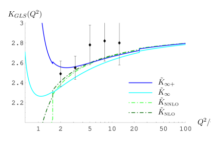
Figure 1: Various predictions for the GLS sum rule, superimposed on to experimental data.

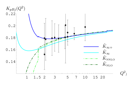
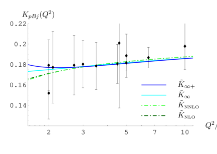
Figure 2: Various predictions for the polarized Bjorken sum rule, superimposed on to experimental data.

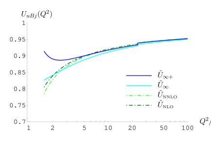
Figure 3: Various predictions for the unpolarized Bjorken sum rule.

We wish to compare these results with relevant experimental data. Data is available for the GLS sum rule [19] and the polarized Bjorken sum rule [20, 21, 22, 23], where the points we plot are those arising from the analysis of [24]. We plot the data in Figs. 1 and 2 along with our predictions for the full observables. No experiment has so far measured the unpolarized Bjorken sum rule, however the possibility exists that it may be extracted from experiments at a future neutrino factory [43]. We have taken ${\Lambda}^{(5)}_{\textrm{\tiny{$\overline{{\rm MS}}$}}}=207$ MeV, corresponding to the world average value ${\alpha}_{s}(M_{Z})=0.1176$ [29].

Within the considerable error bars we see that the different versions of CORGI all fit the data tolerably well. The important conclusion is that below $Q^{2}\sim{5}$ ${\rm{GeV}}^{2}$ the different approaches give drastically different predictions. This indicates that fixed-order perturbation theory cannot be trusted for these lower energies. Even though we have no experimental data points for ${U}_{uBj}(Q^{2})$ we have plotted the different versions of CORGI in Fig. 3. We see that fixed-order perturbation theory cannot be trusted below $Q^{2}\sim{2}$ ${\rm{GeV}}^{2}$. A surprising feature evident from Figs. 1 - 3 is that even at $Q^{2}=2{\rm{GeV}}^{2}$ the fixed-order NLO and NNLO results remain extremely close, leading to the superficial conclusion that fixed-order perturbation theory is working well. In fact as can be seen from Eqs. (54,56) the CORGI invariant $X_{2}$ for both $\mathcal{K}$ and $\mathcal{U}$ changes sign between $N_{f}=4$ and $N_{f}=5$ and so fortuitously is very small in this region. When $X_{3}^{(L)}$ and higher invariants are resummed the potential unreliability of fixed-order perturbation theory is revealed.

We can contrast these CORGI resummations with a leading-$b$ resummation in the $\overline{{\rm MS}}$ scheme. If we choose the scale $\mu=xQ$ we have, analogous to Eq. (45),

$${\mathcal{K}}_{\infty}^{\textrm{\tiny{$\overline{{\rm MS}}$}}}(x) \equiv a(xQ)+\sum_{n=1}^{\infty}k_{n}^{(n)}(x)b^{n}{a}^{n+1}(xQ)$$ (61)

$$= {\mathcal{K}}_{\infty}({a}_{v}(x))\;.$$ (62)

Here $a(xQ)$ denotes the full higher-loop (three-loop if matching to NNLO) $\overline{{\rm MS}}$ coupling at scale $\mu=xQ$, and the $k_{n}(x)$ coefficients are the $\overline{{\rm MS}}$ coefficients with scale $\mu=xQ$. The coupling ${a}_{v}(x)$ is then defined by,

$$\frac{1}{{a}_{v}(x)}=\frac{1}{a(xQ)}-b\left(\ln x+\frac{5}{6}\right)\;.$$ (63)

We can match this all-orders resummation to the exact NLO and NNLO perturbative coefficients, obtaining, in analogy with Eq. (48),

$${\mathcal{K}}^{\textrm{\tiny{$\overline{{\rm MS}}$}}}_{\infty+}(x)={\mathcal{K}}^{\textrm{\tiny{$\overline{{\rm MS}}$}}}_{\infty}(x)+({k}_{1}(x)-b{k}_{1}^{(1)}(x)){a}^{2}(xQ)+({k}_{2}(x)-b^{2}{k}_{2}^{(2)}(x)){a}^{3}(xQ),$$ (64)

where in this $a(Q)$ is the approximated three-loop coupling, given in [29].

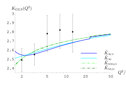
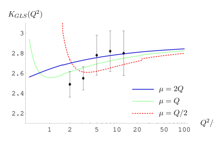
Figure 4: All-orders leading-$b$ prediction for the GLS sum rule. Here we use the $\overline{{\rm MS}}$ result of Eq. (64) with renormalization scales of $\mu=2Q,Q$ and $Q/2$.

The resulting prediction is plotted in Fig. 4 for the GLS sum rule. Three different matching scales corresponding to $x=2,1,\frac{1}{2}$ were chosen. As can be seen, the matched resummed perturbative result is hopelessly $x$-dependent. The CORGI result $\tilde{\mathcal{K}}_{\infty+}(a)$ corresponds to the choice $x={e}^{-{k}_{1}(1)/b}$. However, we note that no NLO matching is required in the CORGI approach, since an infinite set of RG-predictable terms involving $k_{1}$ have been resummed to all-orders, yielding a $\mu$-independent result.

4 Non-perturbative corrections

In addition to perturbative corrections it is expected that there will be non-perturbative, Higher-Twist (HT) corrections to the sum rules. In a recent paper [25] we have studied the infra-red freezing of Euclidean observables, including the sum rules, in the language of the one-chain term of the skeleton expansion. The leading-$b$ resummations we have discussed can be written in the form,

$${\mathcal{K}}_{\infty}(Q^{2})=\int_{0}^{1}{dt}\;{\omega}^{\textrm{\tiny{IR}}}_{\mathcal{K}}(t)a(t{Q}^{2})+\int_{1}^{\infty}{dt}\;{\omega}^{\textrm{\tiny{UV}}}_{\mathcal{K}}(t)a(t{Q}^{2})\;.$$ (65)

Here $\omega_{\mathcal{K}}(t)$ is the characteristic function which is piecewise continuous at $t=1$. The two terms respectively reproduce the IR renormalon and UV renormalon contributions in the Borel sum, but the skeleton expansion result is also defined for $Q^{2}<\Lambda^{2}$ where the standard Borel representation breaks down. Remarkably, there is continuity and finiteness at $Q^{2}=\Lambda^{2}$. By considering the compensation of ambiguities between perturbative and non-perturbative corrections alluded to above we are led to an expression for HT corrections in terms of the characteristic function,

$${\mathcal{K}}_{\textrm{\tiny{HT}}}(Q^{2})=\kappa\frac{{\Lambda}^{2}}{Q^{2}}\omega^{\textrm{\tiny{IR}}}_{\mathcal{K}}\left(\frac{\Lambda^{2}}{Q^{2}}\right)\;.$$ (66)

Here $\kappa$ is a single overall non-perturbative constant. This result is obtained from the V-scheme result of Eq. (31) and hence the appropriate scale parameter for Eq. (66) is $\Lambda_{{\rm V}}$. A similar expression holds for ${\mathcal{U}}_{\textrm{\tiny{HT}}}(Q^{2})$ in terms of ${\omega}^{\textrm{\tiny{IR}}}_{\mathcal{U}}(t)$.

The characteristic functions $\omega_{\mathcal{K}}(t)$ and $\omega_{\mathcal{U}}(t)$ can be determined from their Borel transforms, using a result from [25]. $\omega_{\mathcal{K}}(t)$ has the form,

$$\omega_{\mathcal{K}}^{\textrm{\tiny{IR}}}(t) = \frac{8}{9}-\frac{5}{9}t,$$ (67)

$$\omega_{\mathcal{K}}^{\textrm{\tiny{UV}}}(t) = \frac{4}{9t^{2}}-\frac{1}{9t^{3}},$$ (68)

and the equivalent expression for $\mathcal{U}$ is,

$$\omega_{\mathcal{U}}^{\textrm{\tiny{IR}}}(t) = \frac{4}{3}-t,$$ (69)

$$\omega_{\mathcal{U}}^{\textrm{\tiny{UV}}}(t) = \frac{1}{3t^{3}}.$$ (70)

In Figs. 5 and 6 we take the four expressions in Eqs. (45), (48), (50) and (51), supplemented by the non-perturbative term in Eq. (66), and perform fitting to experimental data for both the GLS and the polarized Bjorken sum rules separately. We fix ${\Lambda}^{(5)}_{\textrm{\tiny{$\overline{{\rm MS}}$}}}=207$ MeV, as before, and use $\chi^{2}$ fitting to obtain the optimal value of the non-perturbative parameters in each case, $\kappa_{GLS}$ and $\kappa_{pBj}$. The fitted parameters are summarized in Table 1. We note that the coefficient of a $1/Q^{2}$ (twist-4) power correction to either Eq. (1) or (2) corresponds to a value of $-8\Lambda_{V}^{2}\kappa_{GLS}/3$ or $-\frac{4}{27}|g_{A}/g_{V}|\Lambda_{V}^{2}\kappa_{pBj}$, respectively. The corresponding values in ${\rm{GeV}}^{2}$ are presented in Table 1. For comparison the central values resulting from a three-point function QCD sum rules fit [44, 45] are $-0.294$ and $-0.013$, respectively. We see that the power corrections in Table 1 resulting from fitting to the resummed ${\tilde{\mathcal{K}}}_{\infty+}(a)$ all-orders resummations are significantly smaller, although the errors are large. Connections between power corrections for the three DIS sum rules have also been explored in [46].

	$\kappa_{GLS}$	$-\frac{8}{3}\kappa_{GLS}\Lambda^{2}_{V}$	$\frac{\chi_{GLS}^{2}}{\rm d.o.f.}$	$\kappa_{pBj}$	$-\frac{4}{27}\left|\frac{g_{A}}{g_{V}}\right|\kappa_{pBj}\Lambda^{2}_{V}$	$\frac{\chi_{pBj}^{2}}{\rm d.o.f.}$
$\tilde{\mathcal{K}}_{\textrm{\tiny{NLO}}}$	-0.166	$0.1007\pm 0.12$	$1.256/4$	-0.06255	$0.002647\pm 0.011$	1.173/11
$\tilde{\mathcal{K}}_{\textrm{\tiny{NNLO}}}$	-0.217	$0.1313\pm 0.12$	$1.238/4$	-0.1085	$0.004593\pm 0.011$	1.162/11
$\tilde{\mathcal{K}}_{\infty}$	-0.33	$0.1997\pm 0.12$	$1.804/4$	-0.2823	$0.01195\pm 0.011$	1.456/11
$\tilde{\mathcal{K}}_{\infty+}$	0.0216	$-0.01311\pm 0.12$	$2.089/4$	0.03957	$-0.001674\pm 0.011$	1.662/11

Table 1: Fitted values of the non-perturbative constants $\kappa_{GLS}$ and $\kappa_{pBj}$, together with their respective $\chi^{2}$ per degree of freedom.

Figure 5: Predictions for the GLS sum rule, including both perturbative and non-perturbative corrections, fitted to the data by varying the parameter $\kappa_{GLS}$.

Figure 6: Predictions for the polarized Bjorken sum rule, including both perturbative and non-perturbative corrections, fitted to the data by varying the parameter $\kappa_{pBj}$.

5 Conclusions

By comparing leading-$b$ resummations based on the CORGI approach we attempted to infer the validity of fixed-order perturbation theory for the GLS and pBj DIS sum rules at small energy scales $Q^{2}\sim{3}\;{\rm{GeV}}^{2}$, where data has previously been used to extract ${\alpha}_{s}(M_{Z})$ [29]. Figures 1 and 2 indicate that fixed-order perturbation theory and resummed all-orders predictions start to differ drastically for energies below $Q^{2}\sim{5}\;{\rm{GeV}}^{2}$. The use of the CORGI approach ensures that all RG-predictable scale-dependent logarithms are resummed to all-orders, thus avoiding the need for NLO matching which would otherwise make the conclusions about the validity of fixed-order perturbation theory dependent on the chosen matching scale (as illustrated in Fig. 4).

We performed fits to data for power corrections using the model proposed in Ref. [25] based on the skeleton expansion characteristic function. The size of power corrections inferred by fitting the all-orders CORGI resummations was much smaller than the central values obtained from three-point QCD sum rule estimates of Refs. [44, 45].

We should note that in a recent interesting paper [15] a renormalon analysis of pBj and GLS sum rules was also carried out. The aim in that case was to perform a sophisticated matching of perturbative and non-perturbative effects in the renormalon subtracted approach.

References

• [1] For a review see: M. Beneke, Phys. Rep. 317, 1 (1999), [hep-ph/9807443]; M. Beneke and V. M. Braun, published in โ€˜The Boris Ioffe Festschrift- At the Frontier of Particle Physics/Handbook of QCDโ€, edited by M. Shifman (World Scientific, Singapore, 2001), [hep-ph/0010208]
• [2] C. N. Lovett-Turner and C. J. Maxwell, Nucl. Phys. B452 (1995) 188, [hep-ph/9505224]
• [3] D. J. Broadhurst and A. G. Grozin, Phys. Rev. D52 (1995) 4082, [hep-ph/9410240].
• [4] M. Beneke and V. M. Braun , Phys. Lett. B348 (1995) 513, [hep-ph/9411229].
• [5] M. Neubert, Phys. Rev. D51 (1995) 5924, [hep-ph/9412265].
• [6] J. Chyla, A. Kataev and S. Larin Phys. Lett. B267 (1991) 269.
• [7] D. G. Tonge and C. J. Maxwell, Nucl. Phys. B481 (1996) 681, [hep-ph/9606392]; D. G. Tonge and C. J. Maxwell, Nucl. Phys. B535 (1998) 19, [hep-ph/9705314].
• [8] D. M. Howe and C. J. Maxwell, Phys. Rev. D70 (2004) 014002. [hep-ph/0303163].
• [9] J. Chyla and A.L. Kataev, Phys. Lett. B297 (1992) 385. [hep-ph/9209213].
• [10] J. Ellis, E. Gardi, M. Karliner and M.A. Samuel, Phys. Lett. B366 (1996) 268. [hep-ph/9609312].
• [11] G. Altarelli, R. D. Ball, S. Forte and G. Ridolfi, Nucl. Phys. B496 (1997) 337. [hep-ph/9701289].
• [12] T. Lee Phys. Rev.D56 (1997) 1091. [hep-ph/9611010]; T. Lee Phys. Lett. B462 (1999) 1. [hep-ph/9908225]
• [13] K. A. Milton, I. L. Solovtsov and O. P. Solovtsova, Phys. Rev. D60 (1999) 016001.
• [14] C. Contreras, G. Cvetic, K. S. Jeong and T. Lee, Phys. Rev. D66, 054006 (2002). [hep-ph/0203201]
• [15] F. Campanario and A. Pineda, Phys. Rev. D72 (2005) 056008. [hep-ph/0508217].
• [16] G. Grunberg, Phys. Lett. B95 (1980) 70; G. Grunberg, Phys. Rev. D29 (1984) 2315.
• [17] C. J. Maxwell [hep-ph/9908463]; C. J. Maxwell and A. Mirjalili, Nucl. Phys. B577 (2000) 209. [hep-ph/0002204].
• [18] C. J. Maxwell and A. Mirjalili, Nucl. Phys. B611 (2001) 423, [hep-ph/0103164].
• [19] J. H. Kim and D. A. Harris et al. Phys. Rev. Lett. 81 (1998) 3595, [hep-ex/9808015].
• [20] K. Abe et al.[E143 collaboration], Phys. Rev.D58, (1998) 112003. [hep-ph/9802357].
• [21] B. Adeva, et al. [Spin Muon Collaboration] Phys. Rev D58 (1998) 112002.
• [22] P. L. Anthony et al. [E155 Collaboration], Phys. Lett.B493 (2000) 19. hep-ph/0007248]
• [23] A. Airapetian et al. [HERMES collaboration], Eur. Phys. J. C26 (2003) 527. [hep-ex/0210047]
• [24] A.ย Deur et al., Phys.ย Rev.ย Lett.ย  93 (2004) 212001. [hep-ex/0407007].
• [25] P.ย M.ย Brooks and C.ย J.ย Maxwell, Phys.ย Rev.ย  D 74 (2006) 065012 [hep-ph/0604267].
• [26] D.ย J.ย Gross and C. H. Llewellyn Smith, Nucl. Phys. B14 (1969) 337.
• [27] J.ย D.ย Bjorken, Phys. Rev. 148 (1966) 1467; D1 (1970) 1376.
• [28] J. D. Bjorken, Phys. Rev. 179 (1969) 1547.
• [29] S.ย Eidelman et al. [Particle Data Group], Phys.ย Lett.ย B 592 (2004) 1.
• [30] S. G. Gorishny and S. A. Larin, Phys. Lett. B172 (1986) 109; S.A. Larin and J. A. M. Vermaseren, Phys. Lett. B259 (1991) 345.
• [31] K. G. Chetyrkin, S. G. Gorishny, S. A. Larin and F. V. Tkachov,Phys. Lett. B137 (1984) 230; S.A. Larin, F. V. Tkachov, and J. A. M. Vermaseren, Phys. Rev. Lett. 66 (1991) 862.
• [32] C.J. Maxwell, Phys. Lett. B409 (1997) 382. [hep-ph/9706231].
• [33] M. Beneke, V. Braun and N. Kivel, Phys. Lett. B404 (1997) 315. [hep-ph/9703389].
• [34] D. J. Broadhurst and A. L. Kataev, Phys. Lett. B315 (1993) 179, [hep-ph/9308274].
• [35] D. J. Broadhurst and A.L. Kataev, Phys. Lett. B544 (2002) 154, [hep-ph/0207267].
• [36] E. Gardi, G. Grunberg and M. Karliner, JHEP 9807 (1998) 007, [hep-ph/9806462].
• [37] M. A. Magradze, Int. J. Mod. Phys. A15, (2000) 2715, [hep-ph/9911456].
• [38] G โ€™t Hooft, in Deeper Pathways in High Energy Physics, proceedings of Orbis Scientiae, 1977, Coral Gables, Florida, edited by A. Perlmutter and L.F. Scott (Plenum, New York, 1977).
• [39] R. M.ย Corless,ย G. H.ย Gonnet,ย D. E. Gย Hare,ย D. J.ย Jeffrey and D. E. Knuth, โ€œOnย the ย Lambertย W๐‘ŠWย functionโ€, Advancesย inย Computationalย Mathematicsย 5ย (1996)ย 329, available from http://www.apmaths.uwo.ca/โˆผsimilar-to\simdjeffrey/offprints.html.
• [40] P. M. Stevenson, Phys. Rev. D23, (1981) 2916.
• [41] G. Grunberg, Phys. Rev. D46 (1992) 2228.
• [42] W. Bernreuther and W Wetzel, Nucl. Phys. B197 (1982) 228; Erratum ibid. B513 (1998) 758.
• [43] S. L. Alekhin and A. L. Kataev, J. Phys. G29 (2003) 1993, [hep-ph/0209165].
• [44] V. M. Braun and A. V. Kolesnichenko, Nucl. Phys. B283 (1987) 723.
• [45] I. L. Balitsky, V. M. Braun and A. V. Kolesnichenko, Phys. Lett.B242 (1990) 245; Erratum ibid. B318 (1993) 648.
• [46] A. L. Kataev, Mod. Phys. Lett. A20 (2005) 2007. [hep-ph/0505230].