1 Introduction

It has been accepted for a long time that hadrons from the same family lie on Regge trajectories (the so-called Chew-Frautschi conjecture [1]), i.e.

$$J=\alpha(0)+\alpha^{{}^{\prime}}M^{2},$$ (1)

where $J$ is the total angular momentum and $M$ is the mass of a hadron. The intercept $\alpha(0)$ depends on hadron type, but the slope $\alpha^{{}^{\prime}}$ is approximately the same for all hadrons. Such a relationship between $J$ and $M^{2}$, also known as the principle of exchange degeneracy, is usually interpreted as a manifestation of the linear potential of the strong forces between constituent quarks. Recently this picture was discussed in terms of a relativistic diquark model based on a spinning string with a constant tension [4, 6, 7] (see also references in [8]).

Experimentally, the validation of Eq. (1) remains to be a difficult problem since the experimental data are scarce. According to a recent classification of hadrons on the ($J,M^{2}$) plane[9], the overwhelming majority of the trajectories are supported by a few data points only. For mesons, there exist five trajectories with three data points, while other trajectories were hypothesized from two or one data points. For baryons, only one trajectory was constructed from four data points and five trajectories were supported by three data points. Other trajectories were hypothesized from the study of either one or two data points. Recently, it has been noted that only $9\%$ ($14\%$) of all trajectories in the mesonic (baryonic) sector are linear [10]. A non-linear character of the Regge trajectories has also been pointed out in [11, 12, 7].

In this article we are not going to scrutinize the linearity of the Regge trajectories; it is rather clear that the vast majority of such trajectories are indeed non-linear and there is no necessity to re-analyse this fact again. Instead, using the most recent PDG data  [13], we would like to note that it is possible to find a prescription which could allow the construction of the trajectories which can be classified as being perfectly linear and span over a significant number of known baryons. In order to illustrate this, we use a rigorous weighted least-squares regression, which is often missing in theoretical papers on this subject. In Sect. 2, we will discuss our principles for the construction of a linear relationship between the hadronic mass squared $M^{2}$ and the total angular momentum $J$. In Sect. 3, our empirical observation is discussed in more details. In particular, we will explain what would happen if the requirements proposed in Sect. 2 are removed or weakened. In Sect. 4 and appendices, we will attempt to use our approach for validation of a relativistic diquark model based on a spinning string, which is often discussed in the literature (see [7] for a recent discussion). Finally, we will briefly discuss the mesonic sector in Sect. 5.

2 Linear trajectories for baryons

As a starting point in the construction of baryonic trajectories, we will consider: (a) only stable or strongly decaying particles from a certain family; (b) only hadrons of the same family with a smallest mass, $M_{min,J}$, for a given fixed $J$ and space parity $P$; (c) in addition to (a) and (b), we will use only such baryons if there are no other baryons with smaller masses and with the opposite space parity. At this moment, we will use the assumptions above without any theoretical justification. Below we will show that, without any exception, such requirements are sufficient for the construction of perfectly linear baryonic trajectories.

As a leading principle for the selection of hadrons, we will ignore particles with poor evidence of existence i.e. with one star in accordance with the PDG classification [13]. Furthermore, in several cases when PDG quotes only mass ranges, we will use the central values for the masses and their experimental errors as they are given by the most accurate and recent measurements.

We will attempt to describe the mass dependence on $J$ using a linear parameterisation similar to Eq. (1):

$$M^{2}_{min,J}=p_{0}+p_{1}J,$$ (2)

where $p_{0}$ and $p_{1}$ are constants. Hereafter we will use the notation $M$ for $M_{min,J}$, unless otherwise stated. For convenience of a linear-regression analysis, we prefer to express $M^{2}$ as a function of $J$ since the angular momentum does not have experimental uncertainties. The linear least-squares regression analysis is described in Appendix A.

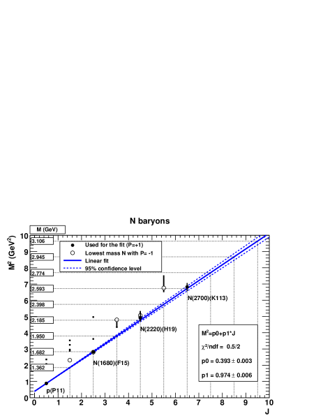
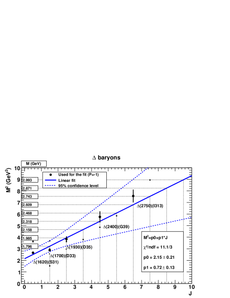
$N$ baryons. First, let us consider $N$ baryons. Figure 1 shows all PDG $N$-baryons on the $(J,M^{2}$) plane (the filled and open symbols). There is a clear linear trend for lowest-mass baryons with $P=+1$ shown by the filled circles (the PDG names of such baryons are indicated). Since such baryons fully satisfy the criteria proposed at the beginning of this section, we will use them for a linear least-squares regression. The result of this regression is shown with the solid line. The trajectory is remarkably straight: the small value of $\chi^{2}/ndf$ shown in Fig. 1 fully supports the linear fit.

To check a possible non-linearity of the $N$-baryon trajectory, a fit was performed using a second-order polynomial function. The inclusion of additional term to the fitting function leads to a small value ($\simeq 0.005$) of the parameter responsible for the quadratic term. However, the quality of such fit characterized by $\chi^{2}/ndf=0.15/1$ does not significantly improve. Two dashed lines shown in Fig. 1 indicate a $95\%$ confidence-level region for the linear regression, assuming that the experimental uncertainties on the masses are normally distributed. This illustrates the reliability of the linear relationship between the $M^{2}$ and $J$ values. From the two tests above, it can be concluded that there is no evidence for non-linearity of the $N$-baryon trajectory.

It should be noted that we do not include the $N(1990)(F17)**$ baryon at $J=7/2$ to the fit. In principle, the quality of the fit will not suffer if the quoted PDG mass ($\simeq 1990{\,\mathrm{MeV}}$) is used. However, if one uses the most recent measurement given by the PDG [14], then the $N(1990)(F17)$ point will move up to the location indicated by the small symbol at $2086\pm 28{\,\mathrm{MeV}}$ (Fig. 1). In this case, this baryon will overlap on the $(J,M^{2}$) plane with a better established $P=-1$ baryon $N(2190)(G17)$, which has a mass of $2190^{+10}_{-90}{\,\mathrm{MeV}}$ (again in accordance with the latest measurement). In this case, $N(1990)(F17)$ should not be used for the fit due to the “lowest-mass” exclusion principle. Since there is no any objective criteria for inclusion (or exclusion) of non-well established $N(1990)(F17)$ baryon to (from) the fit, it was decided to exclude it.

The situation with the lowest-mass $P=-1$ $N$ baryons, shown in Fig. 1 (open symbols), is more complicated and will be discussed in Section 3.

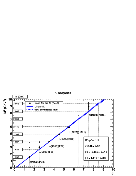
$\Delta$ baryons. Now let us consider the $\Delta$ baryons. Figure 2 shows the $(J,M^{2})$ plane for all $\Delta$ baryons (filled symbols). The filled circles show the $P=+1$ baryons with smallest masses at a given $J$ (their PDG names are indicated). It should be noted that the PDG name for the $\Delta(2000)$ baryon with $J=5/2$ is likely to be inappropriate since most recent experimental studies have indicated that its mass is either $1724\pm 61{\,\mathrm{MeV}}$ [15] or $1752\pm 32{\,\mathrm{MeV}}$ [16]. For the linear fit, we use the former mass, which is also quoted in [14].

The linear least-squares regression for the lowest-mass $\Delta$ baryons with $P=+1$ is shown in Fig. 2 by the solid line. The $\chi^{2}/ndf=6.1/4$ supports the linear fit, despite very small experimental uncertainties on the measured masses and the significant range in $J$. The quality of the linear regression is impressive: The dashed lines indicate a $95\%$ confidence-level interval for the linear regression, which is only $170{\,\mathrm{MeV}}$ wide even for $J=21/2$. Both multiple r-squared and adjusted r-squared are $0.9999$ and the p-value is $6.2\cdot 10^{-9}$. Furthermore, a possible non-linear trend was checked by using a second-order polynomial function. Such a fit has $\chi^{2}/ndf=5.4/3$, while the parameter for the quadratic term was consistent with zero ($0.014\pm 0.017$). Thus, one concludes again that there is no evidence for a non-linear behaviour.

The linear regression has only one significant residual at $J=5/2$ where the measured mass squared is $100{\,\mathrm{MeV}}^{2}$ above the upper $95\%$ confidence-level line. However, as was noted above, the existence of the $\Delta(2000)$ baryon is not well settled (two PDG stars), and its mass needs to be determined more accurately. It should also be noted that only three baryons shown in Fig. 2, $\Delta(1232)$, $\Delta(1950)$ and $\Delta(2420)$, are fairly well studied.

Using the principles outline above, it is impossible to find a sufficient number of $\Delta$ baryons with $P=-1$ for the linear regression fit. This will be discussed in Section 3.

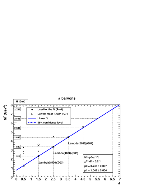
$\Lambda$ baryons. Figure 3 shows the $(J,M^{2})$ plane for all PDG $\Lambda$ baryons (filled symbols). The filled circles show the baryons with the smallest masses and with $P=-1$. Again, such baryons are well described by the linear regression fit ($\chi^{2}/ndf=0.2/1$).

Figure 3 also shows the $\Lambda$ baryons with smallest masses (their names are not indicated) and $P=+1$. The latter baryons ($\Lambda(1115)(P01)$, $\Lambda(1890)(P03)$, $\Lambda(1820)(F05)$ and $\Lambda(2350)(H09)$) cannot be used for the fit since: 1) $\Lambda(1115)(P01)$ decays weakly; 2) the position with $J=3/2$ is already filled with the $\Lambda(1520)(D03)$ baryon which has the opposite parity. We examine this further in Sect. 3.

Other baryons. For $\Omega$ and $\Xi$ baryons, the existing experimental data are insufficient for the construction of the trajectories with more than two data points. The $\Sigma$ baryons will be discussed below.

3 Discussion

It is rather convincing now that the method proposed at the beginning of Sect. 2 indeed works rather well: it allows the construction of three perfectly linear baryonic trajectories with more than two data points. The fit parameters are summarised in Table 1.

Now, let us discuss what would happen if: 1) weakly decaying baryons will be included in the fit as well; 2) one considers baryonic trajectories for a certain parity even when there are baryons with the opposite parity with lower masses. In this context, we will also discuss hadrons with different space parity which have been omitted from the consideration in Section 2. We will not analyse the minimum-mass requirement itself since, without it, the vast majority of baryonic trajectories will be non-linear and identical to those studied elsewhere [8, 10, 11, 12].

First of all, let us include the lowest-mass weakly decaying $\Lambda$ state shown by the open symbol at $J=1/2$ in Figure 3. We will exclude the $\Lambda(1820)(F05)$ state at $J=3/2$, which is also indicated with the open symbol, since this hadron does not satisfy to the minimum-mass criteria. The linear fit of the remaining three baryons, $\Lambda(1115)(P01)$, $\Lambda(1890)(P03)$ and $\Lambda(2350)(H09)$, cannot be considered as a perfect one since $\chi^{2}/ndf=3.2/1$. Thus, the weakly decaying $\Lambda(1115)(P01)$ state violates the linearity.

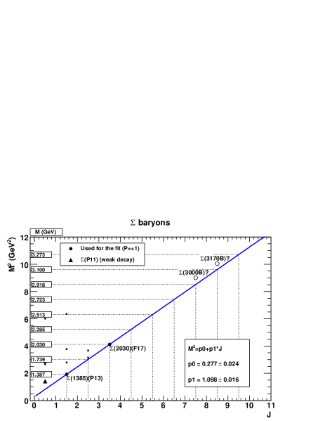
There is a similar situation with the $\Sigma$ baryons. Figure 4 shows the $\Sigma$ baryons with $P=+1$. There are only two points which can be used to construct the trajectory. If the lowest-mass weakly decaying $\Sigma(P11)$ at $J=1/2$ is included, the data points cannot be described by the linear fit.

The open circles in Fig. 4 show two $\Sigma$ baryons whose angular momenta are unknown, but their masses are reasonably well determined. The values of the angular momenta were hypothesized assuming that such baryons should by close to the line determined by $\Sigma(1385)(P13)$ and $\Sigma(2030)(F17)$ baryons. At the same time, these new baryons should be above the $\Delta$-trajectory which bounds the entire baryonic spectra at low masses.

Now let us assume that the minimum-mass requirement for a given parity is not essential in cases when there exist baryons with the opposite parity but with smaller masses for a fixed $J$. First, let us consider the $N$ baryons with $P=-1$ shown in Fig. 1(open symbols). For $J=3/2$ and $11/2$, one can use $N(1520)(D13)$ and $N(2600)(I111)$ baryons without any ambiguity. For $J=5/2$ and $J=9/2$, $N(1675)(D15)$ and $N(2250)(G19)$ baryons with $P=-1$ overlap in masses with the $N$ baryons of the opposite parity, i.e. $N(1680)(F15)$ and $N(2220)(H19)$. If one ignores the minimum-mass requirement, then all baryons indicated by the open symbols should be considered for the regression. Obviously, the linear fit will fail in this case. However, a linear trajectory for the $P=-1$ baryons may still exist if the $N(1675)(D15)$ and $N(2250)(G19)$ states are removed from the consideration on the basis of the minimum-mass requirement.

Now let us consider strongly decaying $\Lambda$ with $P=+1$ shown in Figure 3. It is evident that the data points shown with the open symbols cannot be described by a linear function. Thus, it is essential to exclude $\Lambda(1890)(P03)$ at $J=3/2$ from the consideration. This can indeed be done taking into account the minimum mass requirement and noting the presence of the low-mass $\Lambda(1520)(D03)$ state.

There is another example: $\Delta$ baryons with $P=-1$ (see Fig. 5). Such baryons cannot lie on the same line since the linear fit is characterised by $\chi^{2}/ndf=11/3$ and a wide $95\%$ confidence interval. This can be explained as before: positions with $J=3/2$, $5/2$ and $9/2$ have already been filled with the $P=+1$ baryons with lower masses (shown in Fig. 5 with small filled symbols). Therefore, there are only two baryons left with $J=1/2$ and $11/2$, which is insufficient for the linear regression analysis.

4 Towards extraction of the diquark mass

If our hypothesis is correct, then the present experimental data can be used for the construction only three linear trajectories with more than two data points. All other baryons lying above such trajectories on the $(J,M^{2})$ plane have additional contributions to their masses from non-pure orbital rotations. Perhaps one can use the term “intrinsic noise” [7] for such states: all such hadrons may have a non-linear relationship between $M^{2}$ and $J$ [8, 10, 11, 12].

The linear trajectories proposed above can be used for the validation of a relativistic model in which a hadron can be treated as a rotating flux tube (or a string) with a quark and a diquark at the ends. Such a string can be characterised by a constant tension $T=\sigma/2\pi$. For small (di)quark masses, an approximate solution of this model is given by the Selem-Wilczek (SW) expression [7]:

$$M\simeq\sqrt{\sigma J}+\frac{2}{3}\frac{\pi^{1/2}\mu^{3/2}}{(\sigma J)^{1/4}},\quad\mu^{3/2}=m_{1}^{3/2}+m_{2}^{3/2},$$ (3)

where $m_{1}$ and $m_{2}$ are the masses of diquark and quark connected by a relativistic string. The fitting function directly follows from Eq. (3):

$$M^{2}=\sigma J+\frac{4}{3}\sqrt{\pi\mu^{3}}\cdot(\sigma J)^{1/4}+\frac{4}{9}\frac{\pi\mu^{3}}{\sqrt{\sigma J}}.$$ (4)

This equation resembles the Chew-Frautschi relationship between $M^{2}$ and $J$ in the limit of small masses.

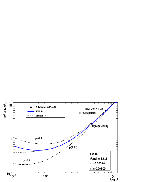
In order to test the model above, we will use the $N$ baryons shown in Figure 1. The fit result using the SW function Eq. (4) is shown in Fig. 6 (solid line), while the two dashed lines illustrate the fit sensitivity to $\mu$ (in this case we keep the slope parameter $\sigma$ to be the same as for the nominal fit using Eq. (4)). The dotted line shows the linear fit as in Figure 1. The fit with the function given in Eq. (4) is strikingly good. The fit parameters are fully constrained by the proton mass at $J=1/2$, since this is exactly the region with a highest sensitivity to $\mu$. The parameter $\sigma$ is $0.908{\,\mathrm{GeV}}^{2}$, which is close to the slope value obtained from the linear fit shown in Figure 1. The extracted value of the mass parameter is $\mu=0.323{\,\mathrm{GeV}}$.

Similar fits have been performed using the $\Delta$ and $\Lambda$ baryons shown in Figures 2 and 3. For such baryons, the fit with Eq. (4) did not converge: the parameter $\mu$ had a fitting error larger than its value and the fit had a significant sensitivity to initial fit values. The reason for this is rather simple: As seen from Fig. 6, the last non-linear term in Eq. (4) can only be constrained by the region $J<1$. However, $\Delta$ and $\Lambda$ trajectories do not have a hadron at such a small $J$. Even although such baryons cannot constrain the mass parameter $\mu$, their linear trajectories are still consistent with a fairly linear behaviour of Eq. (4) at large $J$.

It should be noted that the solution given in Eq. (3) was obtained in the limit of negligible quark masses ($\mu\to 0$) and for large $J$. However, the obtained values of $\mu$ and the range of $J$ used to fit the data may lead to a worry that the above assumptions are not appropriate and the terms beyond ${\cal{O}}(\mu^{3/2})$ are necessary to consider in Eq. (3). Therefore, we have made an attempt to solve the equations of the diquark string model analytically by taking into account high-order terms neglected in the solution [7]. We have obtained a relationship between the mass and $J$ using a full set of ${\cal{O}}(\mu^{3/2})$ terms and, in addition, some terms of order ${\cal{O}}(\mu^{5/2})$ (see Appendix B). It should be stressed that a complete ${\cal{O}}(\mu^{5/2})$ calculation requires a solution of the appropriate quintic equation.

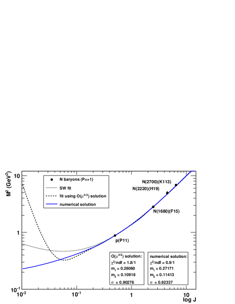
Figure 7 shows the fit using the ${\cal{O}}(\mu^{5/2})$ solution given in Eq. (B-10) of Appendix B. The fit, shown with the dashed line, was performed using three free parameters, $m_{1}$, $m_{2}$ and $\sigma$. It was assumed that the mass of the diquark ($m_{1}$) is larger than that of the quark ($m_{2}$) during the fit. The quality of the fit is fair. It should be noted that if only two parameters are used for the fit, i.e. $\mu$ and $\sigma$ as in the SW case, $\chi^{2}/ndf$ is smaller ($=2.2/2$). In is interesting to observe that $M^{2}$ increases when $J$ decreases. In fact, this is an artifact of truncation of the series in Eq. (B-11); high-order terms proportional to ${\cal{O}}(\mu^{7/2})$ and ${\cal{O}}(\mu^{9/2})$ have negatived contributions and thus turn to reduce the increase of $M^{2}$ at small $J$.

It is rather clear that in order to obtain a reliable model prediction when the masses are not too small, it is essential to find a numerical solution of Eq. (B-5). The result of our numerical calculation used in a $\chi^{2}$-minimisation procedure for the $N$-baryonic trajectory is shown in Figure 7 (the solid line). The fit was found to be excellent.

Table 2 summarizes the fit parameters obtained using different approximations. The numerical solution leads to very similar masses as for the analytical ${\cal{O}}(\mu^{5/2})$ calculation. Moreover, the parameter $\mu\simeq 0.314{\,\mathrm{GeV}}$ calculated from the extracted $m_{1}$ and $m_{2}$ is very similar to that from the SW fit shown in Figure 6. As before, the fit can only be constrained by the $J<1$ region, thus the $N$-baryon trajectory is the most useful for the extraction of the mass parameters and for the validation of this model.

A few words about the precision on the extracted masses are necessary. Table 2 shows the fit values with the necessary numerical precision to reproduce the $\chi^{2}/ndf$ and thus the proton mass, which has a very small experimental uncertainty. The uncertainties on the extracted parameters from the fits are negligible, therefore, they are not quoted (see Appendix A for details). We did not estimate the exact range of the fit parameters which give an acceptable fit (i.e. with $\chi^{2}/ndf<1$) since this will require a significant computational time. However, from several tests we did, we have concluded that the parameters are fairly close to $m_{1}\simeq 0.27\pm 0.01{\,\mathrm{GeV}}$, $m_{2}\simeq 0.11\pm 0.01{\,\mathrm{GeV}}$ and $\sigma\simeq 0.92\pm 0.1{\,\mathrm{GeV}}^{2}$ (the so-called Fit I), with a very strong and complicated correlation between the values.

In addition to the solution given above, we have found another solution with $m_{1}=0.228{\,\mathrm{GeV}}$, $m_{2}=0.179{\,\mathrm{GeV}}$ and $\sigma=0.920{\,\mathrm{GeV}}^{2}$ (Fit II, see Table C-1 of Appendix C), which also gives an acceptable fit, $\chi^{2}/ndf=0.9/1$. In this case, both masses are rather similar, almost in the spirit of the expectations discussed in [7]. This solution corresponds to a different radius of the quark-diquark system (see a discussion in Appendix C). We would like to note that the obtained parameters may not be the only solutions which lead an acceptable fit with $\chi^{2}/ndf<1$, thus the model uncertainties are unknown yet. To find possible alternative solutions will require a significant computational time and, therefore, this is outside of the scope of this paper. The model uncertainties for the $N$-baryon trajectory are further discussed in Appendix C.

It was also verified that if one sets $m_{1}=m_{2}$ for the fit using the numerical solution, then the fit cannot be considered as a good one, $\chi^{2}/ndf\simeq 5/2$. Obviously, the assumption $m_{1}=m_{2}$ is more appropriate for mesons, and it is remarkable that the $N$-baryon trajectory does not support it.

5 Mesons

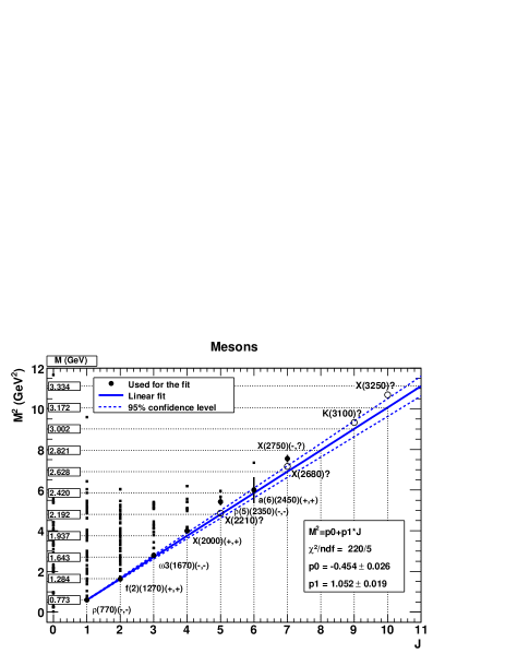
It would be interesting to see the applicability of Eq. (2) and the assumptions discussed in Sect. 2 to the mesonic sector. We will mostly be interested in the linearity of the trajectory which bounds all known mesons on the $(J,M^{2})$ plane at low masses. This is very similar to the $\Delta$ baryons which bound the entire baryonic sector at low masses by the straight trajectory shown in Fig. 2.

Figure 8 shows the $(J,M^{2})$ plane for all PDG mesons (filled symbols). As before, the filled circles show all mesons with lowest masses (for $J\geq 1$) which were used in the linear fit. It can be seen that such mesons approximately lie on a straight line, and this can scarcely be a coincidence. The fit has a significant $\chi^{2}/ndf$ due to very small experimental uncertainties on the measured meson masses, thus one can judge about the linearity only with a certain caution. There is only one significant residual at $J=5$; however, it is not improbable that the $X(2210)$ state may have $J=5$ and thus it falls exactly on the linear fit. All other states indicated with the open circles have unknown $J$ and their locations were hypothesized.

While the slope for the meson sector is somewhat lower, it should be noted that the upper $95\%$ confidence-level line ($p_{0}=-0.503,p_{1}=1.099$) approximately coincides with that for the baryonic sector.

It is interesting to note that there is a clear periodicity in space and charge conjugation parity indicated as ($P,C$) for lowest-mass mesons which bound the meson spectrum on the $(J,M^{2})$ plane (see Fig. 8). This was already noted for the trajectory of vector mesons in [6]. Based on this observation, we can predict that the $C$-parity of $X(2750)$ is likely to be negative.

6 Conclusion

In this paper, using the most recent experimental data, empirical rules have been proposed which are sufficient to reveal a strict linear relationship between the total angular momentum and squared-mass of baryons. Using a least-squares regression, we did not find evidence for non-linearity of such trajectories even when the most stringent statistical tests based on the $\chi^{2}$ and $95\%$ confidence-level intervals were used. In one case, this conclusion was made after the analysis of a number of baryons as large as six. This observation may provide the basis for a new systematization of hadrons and certainly require thoughtful theoretical investigation.

The linear $N$-baryon trajectory can be well described by a semi-classical approach based on a spinning relativistic string with diquark and quark at the ends. We have shown this baryonic trajectory is $\chi^{2}$ consistent with the exact numerical solution of this model (up to nine digits of the extracted model parameters). In this paper we have determined the (di)quark masses from the fit of the $N$-baryon trajectory using our solution.

In principle, this semi-classical model is qualitatively consistent with other linear baryonic trajectories. However, in this paper, we did not attempt to verify this using our numerical calculations. Also, we did not analyse mesons as carefully as baryons. However, it is interesting to observe that the meson spectrum on the $(J,M^{2})$ plane is restricted at small masses by a linear trajectory formed by mesons with $S=C=B=0$ which have periodicity in space and charge conjugation parity.

APPENDIX A

The linear regression was performed using the weights $w=1/\sigma^{2}$, where $\sigma$ is the experimental uncertainty on the mass squared of a hadron. In case of asymmetric experimental errors, we take the average of the upper and the lower experimental uncertainty.

The least-square linear regression was carried out using the R program [18]. The R-package was also used to estimate confidence-level intervals on the linear regression. This package gives larger uncertainties on the linear-regression parameters than the MINUIT program from the CERNLIB FORTRAN library [17]. The MINUIT parameter errors give information on the uncertainty in the best fit values and are not meaningful when points do not have (or have very small) experimental uncertainties.

In contrast to the standard linear least-square regression analysis, the MINUIT program was used for validation of the relativistic string model discussed in Section 4. This simplifies the fit procedure in case of non-linear functions, especially when their analytic form is unknown (as in case of the numerical solution of the string model discussed in Section 4). The extracted fit parameters with the necessary numerical precision to reproduce the proton mass are shown in Table 2. The MINUIT parameter errors are not shown, since they are smaller than the last digit.

APPENDIX B

Here we will derive the functions used to fit the $N$-baryon trajectory shown in Fig. 7. First, recall the main set of equations (8)-(9) of the string model [7]:

$$E = \sum_{n=1}^{2}\Big{(}m_{n}\gamma_{n}+\frac{T}{\omega}\arcsin(\beta_{n})\Big{)},$$ (B-1)

$$J = \sum_{n=1}^{2}\Big{[}\frac{m_{n}}{\omega}\beta^{2}_{n}\gamma_{n}+\frac{T}{2\omega^{2}}\Big{(}\arcsin(\beta_{n})-\frac{\beta_{n}}{\gamma_{n}}\Big{)}\Big{]},$$ (B-2)

$$T = \omega m_{n}\beta_{n}\gamma^{2}_{n},\ \ \ \ n=1,2.$$ (B-3)

Here, $E$ is the energy of the quark-diquark system rotating with an angular momentum $J$, $m_{n}$ denotes the mass of a diquark ($n=1$) and quark ($n=2$), $\omega$ is angular velocity, $T$ is a string tension and $\beta_{n}$ is a linear velocity. The factor $\gamma_{n}$ of a given (di)quark is defined as

$$\gamma_{n}=\frac{1}{\sqrt{1-\omega^{2}r^{2}_{n}}},$$

where $r_{n}$ is a distance from the center of rotation.

Our goal is to find a relationship between the energy $E$ and $J$. Such a relationship has to be expressed in terms of $\sigma=2\pi T$ and $m_{n}$. Excluding terms with $\arcsin(\beta_{n})$ from Eq. (B-1) and using the representation

$$\arcsin(\beta_{n})=\frac{\pi}{2}-\frac{1}{2}\arcsin\Big{(}2\frac{\beta_{n}}{\gamma_{n}}\Big{)},$$

one gets from Eq. (B-1)-(B-3)

$$E = 2\omega J+\frac{m_{1}}{\gamma_{1}}+\frac{m_{2}}{\gamma_{2}},$$ (B-4)

$$J = \frac{1}{2T}\Big{(}\frac{T}{\omega}\Big{)}^{2}\Big{[}\pi+\frac{1}{2}\sum_{n=1}^{2}\Big{(}\frac{2\beta_{n}}{\gamma_{n}}-\arcsin\Big{(}\frac{2\beta_{n}}{\gamma_{n}}\Big{)}\Big{)}\Big{]},$$ (B-5)

$$x_{n} = \frac{1}{\beta_{n}\gamma^{2}_{n}},\ \ \ \ n=1,2.$$ (B-6)

We use Eqs. (B-4)-(B-6) to fit the $N$-baryon trajectory and to extract the parameters $m_{n}$ and $\sigma$ from the data. At fixed $J$, $m_{n}$ and $\sigma$, the equation (B-5) can be solved relative to $\omega$ either numerically, or to some approximation, using a series expansion. Here, $x_{n}=m_{n}\omega/T$ can be used as the expansion variable in the limit of small (di)quark masses.

In terms of $x_{n}$,

$$\frac{1}{\gamma_{n}} = \Big{[}\frac{2x_{n}}{x_{n}+\sqrt{4+x^{2}_{n}}}\Big{]}^{1/2}=x^{1/2}_{n}-\frac{1}{2^{2}}x^{3/2}_{n}+\frac{1}{2^{5}}x^{5/2}_{n}+{\cal{O}}(x^{7/2}_{n}),$$ (B-7)

$$\frac{\beta_{n}}{\gamma_{n}} = \frac{1}{x_{n}}\Big{[}\frac{2x_{n}}{x_{n}+\sqrt{4+x^{2}_{n}}}\Big{]}^{3/2}=x^{1/2}_{n}-\frac{3}{2^{2}}x^{3/2}_{n}+\frac{9}{2^{5}}x^{5/2}_{n}+{\cal{O}}(x^{7/2}_{n}).$$ (B-8)

Using the expansion

$$\arcsin\Big{(}2\frac{\beta_{n}}{\gamma_{n}}\Big{)}=\frac{2\beta_{n}}{\gamma_{n}}+\frac{4}{3}\Big{(}\frac{\beta_{n}}{\gamma_{n}}\Big{)}^{3}+\frac{12}{5}\Big{(}\frac{\beta_{n}}{\gamma_{n}}\Big{)}^{5}+{\cal{O}}(\Big{(}\frac{\beta_{n}}{\gamma_{n}}\Big{)}^{7}),$$

Eq. (B-5) becomes

$$J=\frac{1}{2T}\Big{(}\frac{T}{\omega}\Big{)}^{2}\Big{[}\pi-\frac{2}{3}\Big{(}\frac{\beta_{1}}{\gamma_{1}}\Big{)}^{3}-\frac{2}{3}\Big{(}\frac{\beta_{2}}{\gamma_{2}}\Big{)}^{3}-\frac{6}{5}\Big{(}\frac{\beta_{1}}{\gamma_{1}}\Big{)}^{5}-\frac{6}{5}\Big{(}\frac{\beta_{2}}{\gamma_{2}}\Big{)}^{5}+{\cal{O}}(\Big{(}\frac{\beta_{n}}{\gamma_{n}}\Big{)}^{7})\Big{]}.$$ (B-9)

Thus, substituting Eq. (B-7) and Eq. (B-8) in Eq. (B-4) and Eq. (B-9) and keeping only terms up to order $m^{5/2}_{n}$, one obtains:

$$E = \pi\Big{(}\frac{T}{\omega}\Big{)}+\frac{\mu^{3/2}_{1}}{3}\Big{(}\frac{\omega}{T}\Big{)}^{1/2}+\frac{\mu^{5/2}_{2}}{20}\Big{(}\frac{\omega}{T}\Big{)}^{3/2}+{\cal{O}}(\mu^{7/2}),$$ (B-10)

$$J = \frac{\pi}{2T}\Big{(}\frac{T}{\omega}\Big{)}^{2}-\frac{\mu^{3/2}_{1}}{3T}\Big{(}\frac{\omega}{T}\Big{)}^{-1/2}+\frac{3}{20}\frac{\mu^{5/2}_{2}}{T}\Big{(}\frac{\omega}{T}\Big{)}^{1/2}+{\cal{O}}(\mu^{7/2})$$ (B-11)

with $\mu^{3/2}_{1}=m^{3/2}_{1}+m^{3/2}_{2}$ and $\mu^{5/2}_{2}=m^{5/2}_{1}+m^{5/2}_{2}$.

Let us denote $V=\sqrt{\omega/T}$ and rewrite Eq. (B-11) as a quartic equation

$$V^{4}+aV^{3}-b=0,$$ (B-12)

with

$$a=\frac{2\pi\mu^{3/2}_{1}}{3\sigma J},\ \ \ \ \ \ b=\frac{\pi^{2}}{\sigma J},$$

where the term proportional to $\mu^{5/2}_{2}$ was neglected. To solve the quartic equation (B-12) we use the Ferrari method [19]. The resolvent cubic of Eq. (B-12)

$$U^{3}+4bU+ba^{2}=0,$$ (B-13)

transforms Eq. (B-12) to a quadratic equation:

$$V^{2}+\gamma_{\pm}V+\delta_{\pm}=0$$ (B-14)

with

$$\gamma_{\pm}=\frac{1}{2}[a\pm\sqrt{a^{2}+4U}],\ \ \ \delta_{\pm}=\frac{1}{2}[U\pm\sqrt{U^{2}+4b}],$$ (B-15)

where a real root of Eq. (B-13) (the Cardano formula) is

$$U=\frac{1}{6}\Big{[}12b\sqrt{81a^{4}+768b}-108ba^{2}\Big{]}^{1/3}-\frac{1}{6}\Big{[}12b\sqrt{81a^{4}+768b}+108ba^{2}\Big{]}^{1/3}.$$ (B-16)

Thus, a real and positive solution of Eq. (B-14) and therefore, of Eq. (B-12), is

$$V=\Big{(}\frac{\omega}{T}\Big{)}^{1/2}=\frac{1}{4}\Big{\{}\Big{[}(a^{2}+4U)^{1/2}-a\Big{]}+\sqrt{\Big{[}(a^{2}+4U)^{1/2}-a\Big{]}^{2}+8\Big{[}(U^{2}+4b)^{1/2}-U\Big{]}}\Big{\}}.$$ (B-17)

Substituting the above expression in Eq. (B-10), one obtains a desired relationship between the baryonic mass $M=E$ and variables $J$, $\sigma$ and $m_{n}$.

APPENDIX C

Using a graphical representation of different parts of Eqs. (B-4) and (B-5), it is easy to demonstrate that the string model described by the system of equations Eqs. (B-4)-(B-6) allows several solutions for the (di)quark masses. Such solutions have trajectories with very small (but different) non-linear behaviour.

Let us denote by $\mathrm{Z_{n}}$ the following variables

$$\mathrm{Z_{n}}=\frac{2\beta_{n}}{\gamma_{n}},\ \ \ \ n=1,2$$ (C-1)

and introduce a function

$$\mathrm{F}(\mathrm{Z_{1}},\mathrm{Z_{2}})=\sum_{n=1}^{2}\Big{(}\mathrm{Z_{n}}-\arcsin(\mathrm{Z_{n}})\Big{)}$$ (C-2)

which represents the last term in Eq. (B-5). The variables $\mathrm{Z_{n}}$ have values in the interval $[0,1]$, and are related to the parameters $m_{n}$, $\omega$ and $T$ through the equations Eq. (B-6) and Eq. (B-8). The function $\mathrm{F}(\mathrm{Z_{1}},\mathrm{Z_{2}})$ takes values in the range [$2-\pi,0$]. As shown in Fig. C-1(a), $\mathrm{F}(\mathrm{Z_{1}},\mathrm{Z_{2}})$ is symmetric with respect to the median line $\mathrm{Z_{1}}=\mathrm{Z_{2}}$ and a monotonic function of the both arguments. The main feature of Eq. (B-5) is that the equation $\mathrm{F}(\mathrm{Z_{1}},\mathrm{Z_{2}})=\mathcal{F}$, where $\mathcal{F}$ is a constant, defines an isoline on the surface and at fixed $J$ all the points $\{\mathrm{Z_{1}},\mathrm{Z_{2}}\}$ on this isoline correspond to the same angular velocity $\omega$. In Fig. C-1(a), the isolines are shown as lines between colored bands.

Figure C-1: $\mathrm{F}(\mathrm{Z_{1}},\mathrm{Z_{2}})$ as a function of $\mathrm{Z_{1}}$ and $\mathrm{Z_{2}}$ (left) and $\mathrm{Z_{n}}$ shown as a function of the (di)quark velocity (right).

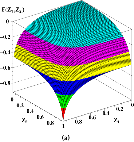
Let us consider the mass evolution equation (B-4) starting from a very high $J$. As follows from (B-5) and the definition of $x_{n}$, a very high $J$ can be obtained only at very small $\omega$ or $x_{n}$. Then Eqs. (B-7) and (B-8) tells that $\gamma_{n}\gg 1$, $\beta_{n}\approx 1$, ${\mathrm{Z_{n}}}\approx 0$ and $\mathrm{F}(\mathrm{Z_{1}},\mathrm{Z_{2}})\approx 0$. Thus, at such $J$, $\beta_{n}$ and $\omega$, the quark and di-quark are at large distances from the center of rotation.

Now, if $J$ decreases and $\omega$, consequently, increases, the phase point $(\mathrm{Z_{1}},\mathrm{Z_{2}})$ on the surface $\mathrm{F}(\mathrm{Z_{1}},\mathrm{Z_{2}})$ is moving along some path in the direction of $(\mathrm{Z_{1}}=1,\mathrm{Z_{2}}=1)$. A fit of the $N$-baryon trajectory fixes a particular path passing at $J=1/2$ through a point $(\mathrm{Z_{1}}^{(f)},\mathrm{Z_{2}}^{(f)})$ on the surface given by $\mathrm{F}(\mathrm{Z_{1}},\mathrm{Z_{2}})$. If $\mathrm{Z_{n}}$ function is plotted as a function of the (di)quark velocity $\beta_{n}$, as shown in Fig. C-1(b), one finds that the point is moving from $\beta\approx 1$ to a smaller $\beta$. The maximum $\mathrm{Z_{n}}=1$ is reached at $\beta_{0}=1/\sqrt{2}$.

	Numerical solution	Numerical solution	limit $\mathrm{Z_{1}}=\mathrm{Z_{2}}=1$,
Parameters	Fit I	Fit II
$\chi^{2}/ndf$	0.9/1	0.9/1	-
$m_{1}$, GeV	0.271713	0.228808	0.18393
$m_{2}$, GeV	0.114134	0.179558	0.18393
$\sigma$, GeV2	0.923374	0.920000	1.12428
$J$	1/2	1/2	1/2
$\omega$, GeV	0.643476	0.628674	0.679332
$\mathrm{Z_{1}}^{(f)}$	0.935557	0.974606	1
$\mathrm{Z_{2}}^{(f)}$	0.975607	0.998309	1
$\mathrm{F}(\mathrm{Z_{1}}^{(f)},\mathrm{Z_{2}}^{(f)})$	-0.648139	-0.884682	2$-\pi$
$x_{1}$	1.189721	0.982401	1/$\sqrt{2}$
$x_{2}$	0.499746	0.770943	1/$\sqrt{2}$
$\beta_{1}$	0.822549	0.782280	1/$\sqrt{2}$
$\beta_{2}$	0.780872	0.727369	1/$\sqrt{2}$
$r_{1}$, GeV-1	1.278291	1.244335	1.045218
$r_{2}$, GeV-1	1.213521	1.156988	1.045218

Table C-1: The model parameters extracted from Eqs. (B-6)-(B-8).

Table C-1 gives the model parameters extracted from Eqs. (B-6)-(B-8) using $m_{n}$ and $\sigma$ found from Fit I and Fit II. First of all, let us note that all $\beta_{n}<1/\sqrt{2}$ (or higher values of $\omega$) correspond to a non-physical $J<1/2$ and $\beta_{n}>1/\sqrt{2}$ holds for the both fits.

The baryon masses predicted by the string model are degenerated with respect to $\omega$ and $m_{n}$. Indeed, $\mathrm{F}(\mathrm{Z_{1}},\mathrm{Z_{2}})$ is negative and, therefore, there is a range of $\omega$ for which one obtains $J_{1}=J_{2}$ at different $\omega_{1}$ and $\omega_{2}$. If (B-5) is equated at different $\omega$, then

$$\frac{1}{\omega^{2}_{1}}[2\pi+\mathcal{F}_{1}]=\frac{1}{\omega^{2}_{2}}[2\pi+\mathcal{F}_{2}]$$ (C-3)

or

$$\mathcal{F}_{2}=\Big{(}\frac{\omega_{2}}{\omega_{1}}\Big{)}^{2}(2\pi+\mathcal{F}_{1})-2\pi.$$ (C-4)

Here $\mathcal{F}_{1}$ and $\mathcal{F}_{2}$ denotes $\mathrm{F}(\mathrm{Z_{1}},\mathrm{Z_{2}})$ at two phase-space points $(\mathrm{Z_{1}},\mathrm{Z_{2}})_{1,2}$. The condition

$$2-\pi\leq\mathcal{F}_{2}\leq 0$$ (C-5)

puts the following restriction on $\omega_{2}$ (at a fixed $\omega_{1}$):

$$\frac{2+\pi}{2\pi+\mathcal{F}_{1}}\leq\Big{(}\frac{\omega_{2}}{\omega_{1}}\Big{)}^{2}\leq\frac{2\pi}{2\pi+\mathcal{F}_{1}}.$$ (C-6)

The condition (C-6) could mean that if one finds a set of parameters $\{m_{1},\,m_{2},\,\sigma\}_{{}_{1}}$ with the evolution along a path $\{\omega,\,\beta_{1},\,\beta_{2}\}_{{}_{1}}$, there should exist another solution $\{m_{1},\,m_{2},\,\sigma\}_{{}_{2}}$ with a different path $\{\omega,\,\beta_{1},\,\beta_{2}\}_{{}_{2}}$. The second found solution for the $N$-baryon trajectory may confirm such interpretation. Thus, we conclude that the model should have an intrinsic uncertainty for the extracted masses depending on the $\mathrm{Z_{1}}$ and $\mathrm{Z_{2}}$ values.

Particle family	$p_{0}$, GeV2	$p_{1}$, GeV2	$\chi^{2}/ndf$
$N$ baryons, $P=+1$	$0.393\pm 0.003$	$0.974\pm 0.006$	0.5/2
$\Delta$ baryons, $P=+1$	$-0.156\pm 0.013$	$1.116\pm 0.006$	6.1/4
$\Lambda$ baryons, $P=-1$	$0.746\pm 0.007$	$1.042\pm 0.004$	0.2/1
$\Sigma$ baryons, $P=+1$	$0.277\pm 0.024$	$1.098\pm 0.016$	-
mesons (lowest mass)	$-0.454\pm 0.026$	$1.052\pm 0.019$	220/5

Table 1: Fit parameters obtained using the linear parameterisation $M^{2}=p_{0}+p_{1}J$ for several hadronic families with the lowest masses on the $(J,M^{2})$ plane. The $\chi^{2}/ndf$ for the $\Sigma$ states is not given since there are only two points for the linear fit (see the text).

Parameters	SW fit	${\cal{O}}(\mu^{3/2})$	${\cal{O}}(\mu^{5/2})$	numerical
		solution	solution	solution
$\sigma$, GeV2	0.908091023	0.889953024	0.902776942	0.923374256
$\mu$, GeV	0.323158469	-	-	-
$m_{1}$, GeV	-	0.302678728	0.280596424	0.271713077
$m_{2}$, GeV	-	0.109731744	0.109180448	0.114133666
$\chi^{2}/ndf$	1.5/2	2.2/1	1.8/1	0.9/1
Mp, GeV
from Eq. (B-4)	0.938272037	0.938272031	0.938272034	0.938272048
Mp, GeV [13]	$0.938272029\pm 0.000000080$

Table 2: Fit parameters obtained using different solutions of the relativistic diquark model (see the text). The $N$-baryon trajectory was used for the fit. The parameter uncertainties are not shown (see Appendix A). The large number of digits, which is necessary to reproduce the quoted $\chi^{2}/ndf$, is due to a large experimental precision on the $N$-baryon masses. The proton mass was calculated from Eq. (B-4) using different approximations and compared with the world average value.

Figure 1: The $(J,M^{2})$ plane for $N$-baryons. The linear fit was performed using the $P=+1$ baryons with smallest masses for a given $J$. The solid line shows the weighted-least squares regression using a linear model and the dashed lines show the corresponding $95\%$ confidence-level interval. The open symbols show lowest-mass baryons with $P=-1$: $N(1520)(D13)$ (with $J=3/2$), $N(1675)(D15)$ (with $J=5/2$), $N(2190)(G17)$ (with $J=7/2$), $N(2250)(G19)$ (with $J=9/2$) and $N(2600)(I111)$ (with $J=13/2$). The $N(1675)(D15)$ state overlaps in mass with the $N(1680)(F15)$ baryon with positive parity.

Figure 2: The ($J,M^{2}$) plane for $\Delta$ baryons with $P=+1$. The filled circles show lowest-mass $\Delta$ baryons used for the linear weighted-least squares regression. The solid line shows the fit, while the dashed line indicates a $95\%$ confidence-level interval. Small filled squares show all other $\Delta$ baryons.

Figure 3: The ($J,M^{2}$) plane for $\Lambda$ baryons with $P=-1$ (filled symbols) and $P=+1$ (open symbols). The latter hadrons correspond to $\Lambda(1115)(P01)$, $\Lambda(1820)(F05)$, $\Lambda(1890)(P03)$ and $\Lambda(2350)(H09)$. The $\Lambda(1820)(F05)$ baryon with $P=+1$ is on top of $\Lambda(1830)(D05)$ with $P=-1$. Small filled squares show all other PDG $\Lambda$ baryons.

Figure 4: The ($J,M^{2}$) plane for $\Sigma$ baryons. The filled circles show the $\Sigma$ baryons with $P=+1$. The filled triangle shows the lowest-mass weakly-decaying $\Sigma$ with $P=+1$, while the small filled squares show all other PDG $\Sigma$ baryons. The open circles indicate possible locations of several high-mass PDG baryons with unknown $J$.

Figure 5: As Fig. 2, but the fit was performed for the lowest-mass $\Delta$ baryons with $P=-1$.

Figure 6: The fit results for leading and daughter nucleons with positive parity. Only baryons with the minimum mass requirement for a given $J$ were used. The solid line indicated the fit by using Eq. (4) (the so-called SW fit) with two free parameters, $\mu$ and $\sigma$. The parameter uncertainties are negligible (not shown). In order to illustrate the fit sensitivity to $\mu$, the dashed lines show the same fit function but with different $\mu$. The dotted line shows the linear fit shown in Fig. 1.

Figure 7: The dotted line shows the SW fit as in Figure 6. The dashed line shows the fit using the solution of the diquark string model calculated up to ${\cal{O}}(\mu^{5/2})$ terms, see Eq. (B-10) of Appendix B. The fit was performed using two mass parameters, $m_{1}$ and $m_{2}$ ($m_{1}>m_{2}$) and a string tension $\sigma$. The solid line shows the fit using the exact numerical solution (see the text). The parameter uncertainties are negligible. Table 2 gives more exact numbers from the fits.

Figure 8: The ($J,M^{2}$) plane for mesons. The filled circles show the mesons with smallest masses and $J\geq 1$ used for a weighted-least squares linear regression (the solid line). The dashed lines indicate a $95\%$ confidence-level interval for the linear regression. For each meson used in the fit, space parity ($P$) and charge conjugation parity ($C$) are indicated in parentheses. Small filled squares show all other PDG mesons and the open circles indicate guessed location of several high-mass mesons with unknown $J$.

References

- [1] G. F. Chew, S. C. Frautschi, Phys. Rev. Lett. 7 (1961) 394
- [2] G. F. Chew, S. C. Frautschi, Phys. Rev. Lett. 8 (1962) 41
- [3] S. Frautschi, Regge Poles and S-Matrix Theory. Benjamin, New York, 1968
- [4] Y. Kalashnikova, A. Nefediev, Y. Simonov, Phys. Rev. D 64 (2001) 014037
- [5] V. L. Morgunov, A. V. Nefediev, Y. A. Simonov, Phys. Lett. B 459 (1999) 653
- [6] L. D. Soloviev, Phys. Rev. D 58 (1998) 035005
- [7] A. Selem, F. Wilczek, Preprint hep-ph/0602128, 2006
- [8] A. Inopin, G. S. Sharov, Phys. Rev. D 63 (2001) 054023
- [9] V. Anisovich, et al., Quark Models and High Energy Collisions. World Scientific Publishing Co. Pte. Ltd, 2004
- [10] A. Inopin, Preprint hep-ph/0012248, 2000
- [11] A. Tang, J. W. Norbury, Phys. Rev. D 62 (2000) 016006
- [12] P. Desgrolard, et al., Eur. Phys. J. C 18 (2001) 555
- [13] PARTICLE DATA GROUP Collaboration, S. Eidelman, et al., Phys. Lett. B 592 (2004) 1
- [14] PARTICLE DATA GROUP Collaboration, S. Eidelman, et al., The Review of particle physics. Computer files (unpublished), available on http://pdg.lbl.gov/
- [15] T. P. Vrana, S. A. Dytman, T. S. H. Lee, Phys. Rept. 328 (2000) 181
- [16] D. M. Manley, E. M. Saleski, Phys. Rev. D 45 (1992) 4002
- [17] CERNLIB, CERN Program Library (unpublished), available on http://cern.ch/cernlib/
- [18] R-library, R-environment for statistical computing and graphics (unpublished), available on http://www.r-project.org/
- [19] E. W. Weisstein, Quartic Equation. From MathWorld: A Wolfram Web Resource (unpublished), available on http://mathworld.wolfram.com/QuarticEquation.html.