Magnetic Stability Analysis for Abelian and Non-Abelian Superconductors

Abstract

We investigate the origin of Abelian and non-Abelian type magnetic instabilities induced by Fermi surface mismatch between the two pairing fermions in a non-relativistic model. The Abelian type instability occurs only in gapless state and the Meissner mass squared becomes divergent at the gapless-gapped transition point, while the non-Abelian type instability happens in both gapless and gapped states and the divergence vanishes. The non-Abelian type instability can be cured in strong coupling region.

I Introduction

The fermion Cooper pairing between different species with mismatched Fermi surfaces, which was discussed in electronic superconductivity many year agosarma ; LO ; FF ; takada , promoted new interest in the study of color superconducting quark matter in compact starshuang ; shovkovy ; alford , asymmetric nuclear matter with proton-neutron pairingsedrakian ; sedrakian2 , and fermionic atom gas with population imbalancepetit ; sheehy ; exp1 ; exp2 .

For color superconducting quark matter with beta equilibrium and charge neutrality, the Sarmasarma or breached pairing(BP)liu or gaplessshovkovy state possesses paramagnetic response to the external color magnetic fields, i.e., the Meissner masses squared of some gluons are negativehuang1 ; casalbuoni ; alford1 ; fukushima . Therefore, the homogeneous and isotropic gapless state is dynamically unstable in weak coupling BCS region, and some spatially inhomogeneous and anisotropic states are energetically favoredgiannakis ; huang2 ; hong ; gorbar ; he1 .

Since the 8th gluon corresponds to the diagonal generator $T_{8}$ in color space, and in an Abelian system the Meissner mass squared is proportional to the superfluid density, the chromomagnetic instability of the 8th gluon in the gapless two flavor color superconductivity and the negative superfluid density in the BP superfluidity are of the same type instabilitieswu ; he2 ; gubankova . Generally, the Abelian type magnetic instability is related to the Fermi surface topologygubankova . In weak coupling region, one branch of fermionic quasiparticle dispersions has two gapless nodes and there are two sharp effective Fermi surfaces in momentum space. In this case, the Meissner mass squared or the superfluid density is negatively divergent at the gapless-gapped transition point where the chemical potential mismatch between the two pairing fermions is equal to the pairing gap. At strong enough coupling, the branch of the gapless fermionic excitation has only one gapless node, and therefore there is only one sharp effective Fermi surface in momentum space. This type of gapless state is free from both Sarma and magnetic instabilitiespao ; kitazawa ; gubankova and is energetically more favored than the mixed phasecaldas and LOFF phaseLO ; FF .

There exists another type of magnetic instability for the 4-7th gluonshuang1 in the two flavor color superconductivity. We call it non-Abelian magnetic instability. Very different from the Abelian instability for the 8th gluon, the Meissner mass squared for the 4-7th gluons is negative in both the gapless and gapped states and is not divergent at the gapless-gapped transition point. It is recently argued that the LOFF state suffers also negative Meissner masses squared for the 4-7th gluons and the gluonic phase will be energetically favored in a wide range of couplinggorbar ; kiriyama .

In this paper, we will show that the non-Abelian instability is related only to the non-Abelian gauge symmetry and is independent of the details of the attractive interaction between the two pairing fermions. Any system which possesses a SU(3) gauge symmetry may suffer this type of magnetic instability. By regarding the gauge field as the pseudo Nambu-Goldstone currenthuang2 , the non-Abelian instability analysis can be applied to the systems of condensed matter or fermionic atom gas where there is no real non-Abelian gauge field. The paper is organized as follows. We present the general treatment for a non-relativistic fermion system in Section II, then investigate the magnetic instabilities in Abelian and non-Abelian cases in Sections III and IV, respectively, and summarize in Section V. We use the natural unit of $c=\hbar=k_{B}=1$ through the paper.

II General Frame

For a non-relativistic fermion system, the partition function of the system can be generally expressed as

$$Z=\int[d\psi^{\dagger}][d\psi]e^{\int_{x}\left[\psi^{\dagger}\left(-\partial_{\tau}+\frac{\nabla^{2}}{2m}+\mu\right)\psi+{\cal L}_{int}\right]}$$ (1)

in the imaginary time formalism of finite temperature field theory with coordinates $x_{\mu}=\left(\tau=it,\ {\bf x}\right)$, where $\int_{x}=\int d^{3}{\bf x}\int_{0}^{\beta}d\tau$ is the space-time integration with $\beta=1/T$ related to the temperature $T$ of the system, $\psi,m$ and $\mu$ are, respectively, the fermion field, mass and chemical potential, and the interaction sector ${\cal L}_{int}$ provides an attractive coupling between the pairing fermions.

Since a fermion can possess possible inner degrees of freedom, the quantities $\psi,m$ and $\mu$ are normally matrices in inner space. To simplify the calculation, we neglect in this paper mass difference and consider only chemical potential difference in the inner space. Generally, due to the introduction of inner degrees of freedom, the system may have some gauge symmetry, such as a SU(3) gauge symmetry which can, for instance, be realized in a ⁴⁰K atom gas with three hyperfine stateshonerkamp . Suppose the system under consideration has a gauge symmetry with $N$ generators $T_{a}(a=1,2,...,N)$, we can introduce a model gauge field $A_{\mu}^{a}(a=1,2,...,N)$ corresponding to the gauge symmetry, and the partition function including the gauge field can then be written as

$$Z=\int[d\psi^{\dagger}][d\psi][dA]e^{S_{A}}e^{\int_{x}\left[\psi^{\dagger}\left(-D_{\tau}+\frac{{\bf D}^{2}}{2m}+\mu\right)\psi+{\cal L}_{int}\right]},$$ (2)

where the gauge field enters the theory via the standard gauge coupling

$$D_{\mu}=\partial_{\mu}-igT_{a}A_{\mu}^{a}$$ (3)

with the gauge coupling constant $g$, and $S_{A}$ is the action for the gauge field sector which is not shown explicitly here.

Due to the attractive interaction between the fermions, the BCS pairing occurs and breaks the gauge symmetry. The order parameter field $\phi$ which describes the spontaneous symmetry breaking is generally a matrix in the inner space. For $\Delta\equiv\left<\phi\right>\neq 0$, the symmetry group of the Lagrangian is spontaneously broken down to some subgroups, and some components of the gauge field corresponding to the broken generators will obtain the so-called Meissner mass via Higgs mechanism.

What we are interested in in this paper is how the Fermi surface mismatch between the pairing fermions affects the behavior of the Meissner mass, especially, whether it is real and physical. When some Meissner masses squared become negative, the system suffers magnetic instability, and the state with gauge field condensation $\langle{\bf A}_{a}\rangle\neq 0$ which breaks the rotational symmetry is energetically more favored than the homogeneous and isotropic state.

The model gauge field $A_{\mu}^{a}$ we introduced above is in fact not necessary for the magnetic instability analysis. If their is no such a gauge field in the theory, for instance in a fermionic atom gas, it can be replaced by the space-time derivative of the phase fluctuation or the Nambu-Goldstone currenthuang2 corresponding to the broken generators. Generally, we can define a local phase transformation by

$${\cal V}(x)=e^{i\sum_{a=1}^{N}\varphi_{a}(x)T_{a}},$$ (4)

where $\varphi_{a}(x)$ can be regarded as the phase field related to the generator $T_{a}$. Applying the above transformation to the fermion field,

$$\psi(x)={\cal V}(x)\chi(x),\ \ \ \psi^{\dagger}(x)=\chi^{\dagger}(x){\cal V}^{\dagger}(x),$$ (5)

we derive the partition function of the system in terms of the fields $\chi$ and $\varphi$,

$$Z=\int[d\chi^{\dagger}][d\chi][d\varphi]e^{\int_{x}\left[\chi^{\dagger}\left(-{\cal D}_{\tau}+\frac{{\bf{\cal D}}^{2}}{2m}+\mu\right)\chi+{\cal L}_{int}\right]},$$ (6)

where the derivative ${\cal D}_{\mu}$ is defined as

$${\cal D}_{\mu}=\partial_{\mu}-iV_{\mu}(x)$$ (7)

with the Nambu-Goldstone current

$$V_{\mu}(x)={\cal V}^{\dagger}(x)(i\partial_{\mu}){\cal V}(x).$$ (8)

To the linear order in the phase field $\varphi$, the Nambu-Goldstone current takes the form

$$V_{\mu}(x)=\sum_{a=1}^{N}\partial_{\mu}\varphi_{a}(x)T_{a}.$$ (9)

From the comparison with the standard gauge coupling (3), the model gauge field $A_{\mu}^{a}$ and the nonzero gauge field condensation $\langle{\bf A}_{a}\rangle\neq 0$ in symmetry breaking state can be replaced, respectively, by the Nambu-Goldstone current $\partial_{\mu}\varphi_{a}$ and its ensemble averagehuang2 ,

$$\langle\nabla\varphi_{a}\rangle\neq 0.$$ (10)

Therefore, even for those systems without real gauge field, the calculation of the Meissner mass for the model gauge field is still meaningful.

The gauge field condensation or spontaneously generated Nambu-Goldstone current can be absorbed into a LOFF state where the order parameter takes the form

$$\left<\phi(x)\right>=e^{-2iT_{a}{\bf q}_{a}\cdot{\bf x}}\Delta,$$ (11)

if we identify the wave vector ${\bf q}_{a}=g\langle{\bf A}_{a}\rangle=\langle\nabla\varphi_{a}\rangle$.

The thermodynamic potential $\Omega$ of the system is a function of the order parameter $\Delta$ and pair momentum ${\bf q}_{a}$, and the physical values of $\Delta$ and ${\bf q}_{a}$ at fixed temperature and chemical potentials in the ground state correspond to the minimum of the thermodynamic potential,

$${\partial\Omega\over\partial\Delta}=0,\ \ \ {\partial^{2}\Omega\over\partial\Delta^{2}}>0,\ \ \ {\partial\Omega\over\partial{\bf q}_{a}}=0,\ \ \ {\partial^{2}\Omega\over\partial{\bf q}_{a}^{2}}>0.$$ (12)

Since $\Omega(\Delta,{\bf q}_{a})$ in the LOFF state can be expanded in powers of ${\bf q}_{a}$ at the vicinity of ${\bf q}_{a}=0$,

$$\Omega(\Delta,{\bf q}_{a})=\Omega(\Delta,0)+\frac{1}{2g^{2}}M^{2}_{ab}{\bf q}_{a}\cdot{\bf q}_{b}+...,$$ (13)

the coefficients $M^{2}_{ab}$ are just the Meissner masses squared matrix for the gauge field. If some of its elements are negative, the LOFF state is energetically favored. For an Abelian system, $T_{a}=1$, such a LOFF state is just the classical single-wave LOFF stateFF ; takada , and for a non-Abelian system, it can be regarded as an extended non-Abelian LOFF statefukus ; hashimoto .

III Abelian Gauge Symmetry

For an Abelian system with two species of fermions ($\psi=\left(\psi_{1},\psi_{2}\right)^{T}$), a U(1) gauge field $A_{\mu}$ can be introduced into the system via the covariant derivative

$$D_{\mu}=\partial_{\mu}-ieA_{\mu}$$ (14)

with gauge coupling $e$, and the attractive interaction between the two species can be modeled by a point interaction with coupling constant $G$,

$${\cal L}_{int}=G\left(\psi^{\dagger}i\varepsilon\psi^{*}\right)\left(\psi^{T}i\varepsilon\psi\right),$$ (15)

where we have assumed that the pairing can occur only between different species of fermions, indicated by the antisymmetric tensor $(\varepsilon)_{\alpha\beta}\equiv\varepsilon_{\alpha\beta}$ in the inner space. The order parameter describing spontaneous U(1) symmetry breaking is defined as the expectation value of the pair field,

$$\Delta=-2G\langle\psi^{T}i\varepsilon\psi\rangle.$$ (16)

In a homogeneous and isotropic superconductor, $\Delta$ can be set to be real.

To see clearly the effect of the Fermi surface mismatch on the Meissner mass, we replace the individual chemical potentials $\mu_{1}$ and $\mu_{2}$ in $\mu=diag(\mu_{1},\mu_{2})$ by the average chemical potential $\bar{\mu}=\left(\mu_{1}+\mu_{2}\right)/2$ and the chemical potential difference $\delta\mu=\left(\mu_{1}-\mu_{2}\right)/2$ and calculate the Meissner mass of the gauge field as a function of the pairing gap $\Delta$ and the mismatch $\delta\mu$ at fixed $\bar{\mu}$.

The way to calculate the Meissner mass is quite standard. We firstly integrate out the fermionic degrees of freedom and then obtain the effective action for the gauge field. With the Nambu-Gorkov field defined as $\Psi=(\psi,\psi^{\dagger})^{T}$, the effective action can be expressed as

$$S_{eff}[A]=S_{A}+\frac{\Delta^{2}}{4G}-\frac{1}{2}\text{ Tr}\ln\left[{\cal S}^{-1}+{\cal A}\right],$$ (17)

where ${\cal S}^{-1}$ is the inverse of the fermion propagator in Nambu-Gorkov space

$${\cal S}^{-1}=\left(\begin{array}[]{cc}-\partial_{\tau}+\frac{\nabla^{2}}{2m}+\mu&i\Delta\varepsilon\\ i\Delta\varepsilon&-\partial_{\tau}-\frac{\nabla^{2}}{2m}-\mu\end{array}\right),$$ (18)

and ${\cal A}$ is a matrix related to the gauge field, ${\cal A}=diag\left({\cal A}^{+},{\cal A}^{-}\right)$ with the elements ${\cal A}^{\pm}$ defined as

$${\cal A}^{\pm}=\pm eA^{0}\mp\frac{e^{2}}{2m}{\bf A}^{2}-\frac{ie}{2m}(\nabla\cdot{\bf A}+{\bf A}\cdot\nabla).$$ (19)

Since we are interested in the Meissner mass which is related to the spatial or magnetic component of the gauge field, we need only the quadratic term in ${\bf A}$ of the effective action,

$$S_{eff}^{(2)}[{\bf A}]=-\frac{1}{2}\sum_{k}A^{i}(-k)\Pi_{ij}(k)A^{j}(k),$$ (20)

where $\sum_{k}=T\sum_{n}\int{d^{3}{\bf k}\over(2\pi)^{3}}$ means fermion frequency summation and vector momentum integration in the momentum space $k_{\mu}=\left(k_{0}=i\omega_{n},{\bf k}\right)$ with $\omega_{n}=2n\pi T$ for bosons and $\omega_{n}=(2n+1)\pi T$ for fermions. The polarization tensor $\Pi_{ij}$ ($i,j=1,2,3$) can be explicitly expressed as

$$\Pi_{ij}(k) = \frac{e^{2}}{2}\sum_{p}\bigg{[}\frac{\delta_{ij}}{m}\text{Tr}\left({\cal S}(p)\Sigma\right)$$

$$+\frac{(2p_{i}-k_{i})(2p_{j}-k_{j})}{4m^{2}}\text{Tr}\left({\cal S}(p){\cal S}(p-k)\right)\bigg{]}$$

with the matrix $\Sigma$ defined as $\Sigma=diag\left(I_{2},-I_{2}\right)$, where $I_{2}$ is the two dimensional identity matrix in the inner space. The Meissner mass of the gauge field is defined as

$$m^{2}_{A}=\frac{1}{2}\lim_{{\bf k}\rightarrow 0}(\delta_{ij}-k_{i}k_{j}/|{\bf k}|^{2})\Pi^{ij}(0,{\bf k}).$$ (22)

Note that the polarization tensor is composed of two parts: The first term is the diamagnetic term which is related to the fermion number density and the second term is the paramagnetic term including the one-loop diagram of the fermion propagator. This behavior is quite different from that of a relativistic systemhuang1 where the one-loop diagram contributes to both diamagnetic and paramagnetic terms. Another convenient way to calculate the Meissner mass is through the potential curvaturefukushima ; he2 ,

$$m^{2}_{A}=\frac{1}{3}\sum_{i,j=1}^{3}\delta_{ij}\frac{\partial^{2}S_{eff}[{\bf A}]}{\partial A_{i}\partial A_{j}}\bigg{|}_{{\bf A}=0}.$$ (23)

Obviously, the two methods are equivalent.

Defining the notation $\epsilon_{\Delta}=\sqrt{\epsilon_{p}^{2}+\Delta^{2}}$ with $\epsilon_{p}={\bf p}^{2}/(2m)-\bar{\mu}$, we can explicitly express the fermion propagator in the Nambu-Gorkov$\otimes$inner space as

$${\cal S}(p)=\left(\begin{array}[]{cccccc}{\cal G}_{+}^{+}&0&0&-i{\cal F}_{+}\\ 0&{\cal G}_{-}^{+}&i{\cal F}_{-}&0\\ 0&-i{\cal F}_{-}&{\cal G}_{-}^{-}&0\\ i{\cal F}_{+}&0&0&{\cal G}_{+}^{-}\end{array}\right),$$ (24)

where the nonzero matrix elements are defined as

$${\cal G}_{\pm}^{\mp}(p) = \frac{i\omega_{n}\pm\delta\mu\mp\epsilon_{p}}{(i\omega_{n}\pm\delta\mu)^{2}-\epsilon_{\Delta}^{2}},$$

$${\cal F}_{\pm}(p) = \frac{\Delta}{(i\omega_{n}\pm\delta\mu)^{2}-\epsilon_{\Delta}^{2}}.$$ (25)

The Meissner mass squared $m_{A}^{2}$ can be decomposed into a diamagnetic part $\left(m_{A}^{2}\right)_{d}$ and a paramagnetic part $\left(m_{A}^{2}\right)_{p}$ which come, respectively, from the first and second terms of the polarization tensor,

$$m_{A}^{2}=\left(m_{A}^{2}\right)_{d}+\left(m_{A}^{2}\right)_{p}.$$ (26)

After a straightforward algebra, they can be evaluated as

$$\left(m_{A}^{2}\right)_{d} = \frac{e^{2}}{2m}\sum_{p}\Big{[}\left({\cal G}_{-}^{+}+{\cal G}_{+}^{+}\right)e^{i\omega_{n}0^{+}}$$

$$-\left({\cal G}_{-}^{-}+{\cal G}_{+}^{-}\right)e^{i\omega_{n}0^{-}}\Big{]},$$

$$\left(m_{A}^{2}\right)_{p} = \frac{e^{2}}{2m^{2}}\sum_{p}\frac{{\bf p}^{2}}{3}\Big{[}{\cal G}_{-}^{+}{\cal G}_{-}^{+}+{\cal G}_{+}^{+}{\cal G}_{+}^{+}+{\cal G}_{+}^{-}{\cal G}_{+}^{-}$$ (27)

$$+\ {\cal G}_{-}^{-}{\cal G}_{-}^{-}+2{\cal F}_{-}{\cal F}_{-}+2{\cal F}_{+}{\cal F}_{+}\Big{]}.$$

Note that we have added the convergent factors in the Matsubara frequency summation in the diamagnetic part to ensure the condition $m_{A}^{2}(\Delta=0)=0$.

After the Matsubara frequency summation, we obtain

$$\left(m_{A}^{2}\right)_{d} = \frac{e^{2}}{m}\int_{0}^{\infty}\frac{p^{2}dp}{2\pi^{2}}\left[1-{\epsilon_{p}\over\epsilon_{\Delta}}\Theta\left(\epsilon_{\Delta}-\delta\mu\right)\right],$$

$$\left(m_{A}^{2}\right)_{p} = -\frac{e^{2}}{m^{2}}\int_{0}^{\infty}\frac{p^{4}dp}{6\pi^{2}}\delta(\epsilon_{\Delta}-\delta\mu)$$ (28)

at $T=0$. The diamagnetic mass is only related to the number density $n$,

$$\left(m_{A}^{2}\right)_{d}=\frac{ne^{2}}{m},$$ (29)

and the paramagnetic mass can be evaluated as

$$\left(m_{A}^{2}\right)_{p}=-\frac{e^{2}}{m}\frac{\delta\mu\Theta(\delta\mu-\Delta)}{\sqrt{\delta\mu^{2}-\Delta^{2}}}\frac{p_{-}^{3}\Theta\left(\mu_{-}\right)+p_{+}^{3}\Theta\left(\mu_{+}\right)}{6\pi^{2}}$$ (30)

with the definitions

$$p_{\pm}=\sqrt{2m\mu_{\pm}},\ \ \ \mu_{\pm}=\bar{\mu}\pm\sqrt{\delta\mu^{2}-\Delta^{2}}.$$ (31)

In weak coupling region, we have $\bar{\mu}\gg\delta\mu$ and

$$n\simeq\frac{p_{+}^{3}+p_{-}^{3}}{6\pi^{2}}\simeq\frac{(2m\bar{\mu})^{3/2}}{3\pi^{2}},$$ (32)

and the Meissner mass squared can be approximately expressed as

$$m_{A}^{2}=\frac{ne^{2}}{m}\left[1-\frac{\delta\mu\Theta(\delta\mu-\Delta)}{\sqrt{\delta\mu^{2}-\Delta^{2}}}\right].$$ (33)

In the gapless state with $\delta\mu>\Delta$, the Meissner mass squared is negative, and there is a discontinuity at the gapless-gapped transition point $\delta\mu=\Delta$. This divergence and discontinuity come from the delta function in (III).

When the coupling becomes strong enough, the system will enter the BEC region and we have $\bar{\mu}<0$. In this case there is only one gapless node $p_{+}$ and the Meissner mass squared reads

$$m_{A}^{2}=\frac{ne^{2}}{m}\left[1-\frac{\delta\mu\Theta(\delta\mu-\Delta)}{\sqrt{\delta\mu^{2}-\Delta^{2}}}\frac{p_{+}^{3}\Theta\left(\mu_{+}\right)}{6\pi^{2}n}\right].$$ (34)

For $\bar{\mu}<0$, $p_{+}$ becomes much smaller than the Fermi momentum $p_{F}=(3\pi^{2}n)^{1/3}$, the Meissner mass squared in the gapless phase can be positivepao ; gubankova , and the divergence at the gapless-gapped transition point disappears due to the fact that at $\delta\mu=\Delta$ both $p_{+}$ and $p_{-}$ become imaginary. In Fig.1, we plot the Meissner mass squared in BCS and BEC cases. In BCS case, the gapless state suffers magnetic instability, while in the strong coupling BEC region, the instability is fully cured.

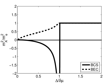
Figure 1: The Meissner mass squared, scaled by $m_{e}^{2}=ne^{2}/m$, as a function of $\Delta/\delta\mu$. We take $\bar{\mu}=0.99\epsilon_{F},\Delta=0.05\epsilon_{F}$ in the BCS case and $\bar{\mu}=-0.1\epsilon_{F},\Delta=0.5\epsilon_{F}$ in the BEC case with $\epsilon_{F}$ being the Fermi energy for free fermions.

IV Non-Abelian Symmetry

In this section we consider a system with two types of inner degrees of freedom which we call color and flavor. They can also be interpreted as spin, isospin and hyperfine state in different systems. Suppose there are two flavors and three colors, like two flavor QCD, the system can be modelled by the partition function

$$Z = \int[d\psi^{\dagger}][d\psi][dA]e^{S_{A}}\times$$

$$e^{\int_{x}\left[\psi^{\dagger}\left(-D_{\tau}+\frac{{\bf D}^{2}}{2m}+\mu\right)\psi+G(\psi^{\dagger}\varepsilon\epsilon^{c}\psi^{*})(\psi^{T}\varepsilon\epsilon^{c}\psi)\right]},$$

where $(\varepsilon)_{\alpha\beta}\equiv\varepsilon_{\alpha\beta}$ and $(\epsilon^{c})^{ab}\equiv\epsilon^{abc}$ are antisymmetric matrices in the flavor and color spaces with the flavor index denoted by $\alpha,\beta$ and color by $a,b,c$. We have introduced a SU(3) gauge field $A_{\mu}^{a}$ corresponding to the color degree of freedom via the derivative $D_{\mu}$ in (3).

We consider pairing only between fermions with different flavors and colors and introduce the order parameter

$$\Delta=-2G\langle\psi^{T}\varepsilon\epsilon^{3}\psi\rangle$$ (36)

which spontaneously breaks the symmetry from SU(3) to SU(2), where we have assumed that only the first two colors participate in the condensate, while the third one does not. Similar to the treatment in Abelian case, we obtain the effective action (17) for the gauge field with the inverse fermion propagator in Nambu-Gorkov space

$${\cal S}^{-1}=\left(\begin{array}[]{cc}-\partial_{\tau}+\frac{\nabla^{2}}{2m}+\mu&\Delta\varepsilon\epsilon^{3}\\ \Delta\varepsilon\epsilon^{3}&-\partial_{\tau}-\frac{\nabla^{2}}{2m}-\mu\end{array}\right)$$ (37)

and the gauge field elements

$${\cal A}^{\pm}=\pm gT_{a}A_{a}^{0}\mp\frac{g^{2}T_{a}^{2}}{2m}{\bf A}_{a}^{2}-\frac{igT_{a}}{2m}(\nabla\cdot{\bf A}_{a}+{\bf A}_{a}\cdot\nabla).$$ (38)

If the fermion chemical potential is color independent, we have $\mu=diag\left(\bar{\mu}+\delta\mu,\bar{\mu}-\delta\mu\right)\otimes I_{3}$ with $I_{3}$ being the three dimensional identity matrix in the color space, the Fermi surface mismatch between the pairing fermions does not break the $SU(3)$ gauge symmetry explicitly, and the quadratic term of the effective action for the magnetic component of the gauge field reads

$$S_{eff}^{(2)}[{\bf A}]=-\frac{1}{2}\sum_{k}A^{i}_{a}(-k)\Pi_{ab}^{ij}(k)A^{j}_{b}(k)$$ (39)

with the polarization tensor

$$\Pi_{ab}^{ij}(k) = \frac{g^{2}}{2}\sum_{p}\bigg{[}\frac{\delta_{ij}\delta_{ab}}{m}\text{Tr}[{\cal S}(p)\Sigma_{a}]$$

$$+\frac{(2p_{i}-k_{i})(2p_{j}-k_{j})}{4m^{2}}\text{Tr}[{\cal S}(p)\Gamma_{a}{\cal S}(p-k)\Gamma_{b}]\bigg{]},$$

where the matrices $\Sigma_{a}$ and $\Gamma_{a}$ are defined as $\Sigma_{a}=diag\left(I_{2}\otimes T_{a}^{2},-I_{2}\otimes T_{a}^{2}\right)$ and $\Gamma_{a}=diag\left(I_{2}\otimes T_{a},I_{2}\otimes T_{a}\right)$.

In the 12-dimensional Nambu-Gorkov$\otimes$flavor$\otimes$color space, the fermion propagator can be explicitly expressed as

$${\cal S}(p) = \left(\begin{array}[]{cccccccccccc}{\cal G}_{+}^{+}&0&0&0&0&0&0&0&0&0&-{\cal F}_{+}&0\\ 0&{\cal G}_{+}^{+}&0&0&0&0&0&0&0&{\cal F}_{+}&0&0\\ 0&0&{\cal G}_{0+}^{-}&0&0&0&0&0&0&0&0&0\\ 0&0&0&{\cal G}_{-}^{+}&0&0&0&{\cal F}_{-}&0&0&0&0\\ 0&0&0&0&{\cal G}_{-}^{+}&0&-{\cal F}_{-}&0&0&0&0&0\\ 0&0&0&0&0&{\cal G}_{0-}^{-}&0&0&0&0&0&0\\ 0&0&0&0&-{\cal F}_{-}&0&{\cal G}_{-}^{-}&0&0&0&0&0\\ 0&0&0&{\cal F}_{-}&0&0&0&{\cal G}_{-}^{-}&0&0&0&0\\ 0&0&0&0&0&0&0&0&{\cal G}_{0-}^{+}&0&0&0\\ 0&{\cal F}_{+}&0&0&0&0&0&0&0&{\cal G}_{+}^{-}&0&0\\ -{\cal F}_{+}&0&0&0&0&0&0&0&0&0&{\cal G}_{+}^{-}&0\\ 0&0&0&0&0&0&0&0&0&0&0&{\cal G}_{0+}^{+}\end{array}\right)$$ (53)

with the elements ${\cal G}^{\mp}_{\pm},{\cal F}_{\pm}$ shown in (III) and the propagator ${\cal G}^{\mp}_{0\pm}$ for the unpaired fermions defined as

$${\cal G}_{0\pm}^{\mp}=\frac{1}{i\omega_{n}\pm\delta\mu\mp\epsilon_{p}}.$$ (54)

Since in the phase with nonzero condensate there is still the symmetry SU(2), only the generators $T_{4},T_{5},T_{6},T_{7},T_{8}$ are broken, we need to calculate the Meissner mass squared only for $a=4,5,6,7,8$.

With the definition for the Meissner mass squared in non-Abelian case,

$$\left(m^{2}_{A}\right)_{ab}=\frac{1}{3}\sum_{i,j=1}^{3}\delta_{ij}\frac{\partial^{2}S_{eff}[{\bf A}]}{\partial A_{i}^{a}\partial A_{j}^{b}}\bigg{|}_{{\bf A}=0},$$ (55)

we first consider $a=4,5,6,7$. It is straightforward to see that all the off-diagonal elements of the matrix $\left(m_{A}^{2}\right)_{ab}$ in the color subspace vanish and the diagonal elements are the same,

$$\left(m^{2}_{A}\right)_{44}=\left(m_{A}^{2}\right)_{55}=\left(m_{A}^{2}\right)_{66}=\left(m_{A}^{2}\right)_{77}.$$ (56)

Therefore, we need to evaluate $m_{A,4}^{2}\equiv\left(m_{A}^{2}\right)_{44}$ only. Taking into account the decomposition,

$$m_{A,4}^{2}=\left(m_{A,4}^{2}\right)_{d}+\left(m_{A,4}^{2}\right)_{p},$$ (57)

the diamagnetic and paramagnetic parts coming, respectively, from the first and second terms of the polarization tensor read

$$\left(m_{A,4}^{2}\right)_{d} = \frac{g^{2}}{8m}\sum_{p}\Big{[}\left({\cal G}_{0-}^{-}+{\cal G}_{0+}^{-}+{\cal G}_{-}^{+}+{\cal G}_{+}^{+}\right)e^{i\omega_{n}0^{+}}$$

$$-\left({\cal G}_{0-}^{+}+{\cal G}_{0+}^{+}+{\cal G}_{-}^{-}+{\cal G}_{+}^{-}\right)e^{i\omega_{n}0^{-}}\Big{]},$$

$$\left(m_{A,4}^{2}\right)_{p} = \frac{g^{2}}{4m^{2}}\sum_{p}\frac{{\bf p}^{2}}{3}\Big{[}{\cal G}_{0-}^{+}{\cal G}_{-}^{-}+{\cal G}_{0-}^{-}{\cal G}_{-}^{+}$$ (58)

$$+\ {\cal G}_{0+}^{+}{\cal G}_{+}^{-}+{\cal G}_{0+}^{-}{\cal G}_{+}^{+}\Big{]}.$$

Note that only the loops with an unpaired fermion and a paired fermion contribute to the paramagnetic term. After the Matsubara frequency summations, we obtain

$$\left(m_{A,4}^{2}\right)_{d} = \frac{g^{2}}{2m}\int_{0}^{\infty}\frac{p^{2}dp}{2\pi^{2}}\left[\Theta(\delta\mu-\epsilon_{p})+\Theta(-\delta\mu-\epsilon_{p})+\frac{\epsilon_{p}}{\epsilon_{\Delta}}\Theta(\delta\mu-\epsilon_{\Delta})+\left(1-\frac{\epsilon_{p}}{\epsilon_{\Delta}}\right)\right],$$

$$\left(m_{A,4}^{2}\right)_{p} = -\frac{g^{2}}{m^{2}}\int_{0}^{\infty}\frac{p^{4}dp}{3\pi^{2}}\left[\frac{\epsilon_{p}}{\Delta^{2}}\left(\Theta(\delta\mu-\epsilon_{p})+\Theta(-\delta\mu-\epsilon_{p})\right)+\left(\frac{1}{\epsilon_{\Delta}+\epsilon_{p}}-\frac{1}{2\epsilon_{\Delta}}\right)-\left(\frac{\epsilon_{\Delta}}{\Delta^{2}}-\frac{1}{2\epsilon_{\Delta}}\right)\Theta(\delta\mu-\epsilon_{\Delta})\right]$$

at $T=0$. At weak coupling, the integrals can be approximately evaluated and the final result is simplified as

$$m_{A,4}^{2}=2m_{g}^{2}\left[\frac{1}{2}-\frac{\delta\mu^{2}}{\Delta^{2}}+\frac{\delta\mu^{2}}{\Delta^{2}}\frac{\sqrt{\delta\mu^{2}-\Delta^{2}}}{\delta\mu}\Theta(\delta\mu-\Delta)\right],$$ (59)

where $m_{g}^{2}=ng^{2}/m$ is a $\Delta$ and $\delta\mu$ independent constant.

In Fig.2, we show the Meissner mass squared $m_{A,4}^{2}$ as a function of the gap parameter $\Delta$. In the BCS case, both the gapless state in the region $\Delta/\delta\mu<1$ and the gapped state in the region $1<\Delta/\delta\mu<\sqrt{2}$ suffer magnetic instability, and the Meissner mass squared is continuous at $\Delta/\delta\mu=1$. The continuity at the gapless-gapped transition point is totally different from the case with Abelian symmetry. We also observed that the magnetic instability can be cured in the strong coupling BEC region.

Now we turn to the calculation of the Meissner mass squared with $a=8$. Again we make the diamagnetic and paramagnetic decomposition,

$$m_{A,8}^{2}\equiv\left(m_{A}^{2}\right)_{88}=\left(m_{A,8}^{2}\right)_{d}+\left(m_{A,8}^{2}\right)_{p},$$ (60)

and each part can further be divided into a unpaired fermion term and a paired fermion term,

$$\left(m_{A,8}^{2}\right)_{d} = \left(m_{A,8}^{2}\right)_{d}^{0}+\left(m_{A,8}^{2}\right)_{d}^{\Delta},$$

$$\left(m_{A,8}^{2}\right)_{p} = \left(m_{A,8}^{2}\right)_{p}^{0}+\left(m_{A,8}^{2}\right)_{p}^{\Delta}$$ (61)

with the unpaired fermion contributions

$$\left(m_{A,8}^{2}\right)_{d}^{0} = \frac{g^{2}}{8m}\sum_{p}\frac{4}{3}\Big{[}\left({\cal G}_{0-}^{-}+{\cal G}_{0+}^{-}\right)e^{i\omega_{n}0^{+}}$$

$$-\left({\cal G}_{0-}^{+}+{\cal G}_{0+}^{+}\right)e^{i\omega_{n}0^{-}}\Big{]},$$

$$\left(m_{A,8}^{2}\right)_{p}^{0} = \frac{g^{2}}{8m^{2}}\sum_{p}\frac{{\bf p}^{2}}{3}\frac{4}{3}\Big{[}{\cal G}_{0-}^{-}{\cal G}_{0-}^{-}+{\cal G}_{0+}^{-}{\cal G}_{0+}^{-}$$ (62)

$$+{\cal G}_{0-}^{+}{\cal G}_{0-}^{+}+{\cal G}_{0+}^{+}{\cal G}_{0+}^{+}\Big{]},$$

and the paired fermion contributions

$$\left(m_{A,8}^{2}\right)_{d}^{\Delta} = \frac{g^{2}}{8m}\sum_{p}\frac{2}{3}\Big{[}\left({\cal G}_{-}^{+}+{\cal G}_{+}^{+}\right)e^{i\omega_{n}0^{+}}$$

$$-\left({\cal G}_{-}^{-}+{\cal G}_{+}^{-}\right)e^{i\omega_{n}0^{-}}\Big{]},$$

$$\left(m_{A,8}^{2}\right)_{p}^{\Delta} = \frac{g^{2}}{8m^{2}}\sum_{p}\frac{{\bf p}^{2}}{3}\frac{2}{3}\Big{[}{\cal G}_{-}^{+}{\cal G}_{-}^{+}+{\cal G}_{+}^{+}{\cal G}_{+}^{+}+{\cal G}_{+}^{-}{\cal G}_{+}^{-}$$ (63)

$$+{\cal G}_{-}^{-}{\cal G}_{-}^{-}+2{\cal F}_{-}{\cal F}_{-}+2{\cal F}_{+}{\cal F}_{+}\Big{]}.$$

The terms $\left(m_{A,8}^{2}\right)_{d}^{0}$ and $\left(m_{A,8}^{2}\right)_{p}^{0}$ cancel to each other,

$$\left(m_{A,8}^{2}\right)_{d}^{0}+\left(m_{A,8}^{2}\right)_{p}^{0}=0,$$ (64)

which means that the unpaired fermions have no contribution to the Meissner effect corresponding to the 8th gauge field, and the final expression of $m_{A,8}^{2}$ is the same as that in the Abelian case except for a constant factor,

$$m_{A,8}^{2}=\frac{g^{2}}{6e^{2}}m_{A}^{2}.$$ (65)

Therefore, the magnetic stability analysis for the 8th gluon should be the same as the one in the Abelian model.

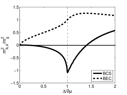
Figure 2: The Meissner mass squared $m_{A,4}^{2}$, scaled by $m_{g}^{2}=ng^{2}/m$, as a function of $\Delta/\delta\mu$. We take $\bar{\mu}=0.99\epsilon_{F},\Delta=0.05\epsilon_{F}$ in the BCS case and $\bar{\mu}=-0.1\epsilon_{F},\Delta=0.5\epsilon_{F}$ in the BEC case.

V Summary

We have investigated the origin of two types of magnetic instabilities induced by the Fermi surface mismatch between the two pairing fermions in a U(1) Abelian model and a SU(3) non-Abelian model. Our results show that the two types of instabilities are very different. The Abelian instability occurs only in the gapless state where the chemical potential mismatch $\delta\mu$ is larger than the gap $\Delta$, and the Meissner mass squared becomes divergent at the gapless-gapped transition point $\delta\mu=\Delta$. However, the non-Abelian instability occurs in both gapless and gapped states, and there is no singularity at the gapless-gapped transition point. In non-Abelian systems, there are both Abelian and non-Abelian magnetic instabilities. The former corresponds to the broken diagonal generators and the latter to those broken off-diagonal generators. While only the paired fermions contribute to the Abelian instability, both paired and unpaired fermions contribute to the non-Abelian instability which leads to the continuity of the Meissner mass squared at the gapless-gapped transition point.

Since the non-relativistic model we considered in this paper has the simple but essential pairing structure and good ultraviolet behavior, it is quite convenient to study the non-Abelian LOFF statefukus ; hashimoto and discuss the competition between the Abelian and non-Abelian LOFF stateskiriyama .

Our investigation indicates that the magnetic instability induced by mismatched fermi surfaces does not depend on the details of the attractive interaction and whether the system is relativistic or non-relativistic. The instability is controlled by the symmetry of the system. While a relativistic and a non-relativistic Fermi gas may have different dynamics, their magnetic instabilities are very similar if they have the same symmetry. For instance, the chromomagnetic instability discovered in relativistic color superconductor may be closely related to the experiments in non-relativistic and non-Abelian condensed matter such as the three-component Fermi gas, and other new discoveries in the study of color superconductivity, such as the abnormal number of Nambu-Goldstone bosonsblaschke ; he3 ; ebert and the instability induced by the mismatch between paired and unpaired fermionshe4 , may be realized in condensed matter systems.

Acknowledgments:  The work was supported in part by the grants NSFC10575058, 10425810, 10435080 and SRFDP20040003103.

References

- (1) G.Sarma, J.Phys.Chem.Solid 24,1029(1963).
- (2) A.I.Larkin and Yu.N.Ovchinnikov, Sov.Phys. JETP 20, 762(1965).
- (3) P.Fulde and R.A.Ferrell, Phys. Rev 135, A550(1964).
- (4) S.Takada and T.Izuyama, Prog.Theor.Phys.41, 635(1969).
- (5) W.V.Liu and F.Wilczek, Phys. Rev. Lett.90, 047002(2003).
- (6) M.Huang, P.Zhuang, and W.Chao, Phys. Rev. D67, 065015(2003).
- (7) I.Shovkovy and M.Huang, Phys. Lett. B564 205(2003).
- (8) M.Alford, C.Kouvaris and K. Rajagopal, Phys. Rev. Lett. 92, 222001(2004).
- (9) A.Sedrakian and U.Lombardo, Phys. Rev. Lett. 84, 602(2000).
- (10) A.Sedrakian and J.W.Clark, nucl-th/0607028.
- (11) A.Sedrakian, J.Mur-Petit, A.Polls and H.M ther, Phys.Rev. A72, 013613(2005).
- (12) D.E.Sheehy and L.Radzihovsky, Phys.Rev.Lett. 96, 060401(2006); cond-mat/0607803.
- (13) M.W.Zwierlein, A.Schirotzek, C.H.Schunck and W.Ketterle, Science 311, 492(2006).
- (14) G.B.Partridge, W.Li, R.I.Kamar, Y.Liao and R.G.Hulet, Science 311, 503(2006).
- (15) M.Huang and I.Shovkovy, Phys. Rev. D70, R051501(2004).
- (16) R.Casalbuoni, R.Gatto, M.Mannarelli, G.Nardulli and M.Ruggieri, Phys. Lett. B605 362(2005).
- (17) M.Alford, Q.Wang, J. Phys. G31 719(2005).
- (18) K.Fukushima, Phys. Rev. D72, 074002(2005).
- (19) I.Giannakis and H.Ren, Phys. Lett. B611, 137(2005); Nucl. Phys. B723, 255(2005); I.Giannakis, D.Hou and H.Ren, Phys. Lett. B631 16(2005).
- (20) M.Huang, Phys. Rev. D73, 045007(2006).
- (21) D.Hong, hep-ph/0506097.
- (22) E.V.Gorbar, M.Hashimoto and V.A.Miransky, Phys. Lett. B632, 305(2006); Phys. Rev. Lett. 96, 022005 (2006).
- (23) L.He, M.Jin and P.Zhuang, Phys. Rev. B73, 214527(2006); cond-mat/0606322.
- (24) S.T.Wu and S.Yip, Phys. Rev. A67, 053603(2003).
- (25) L.He, M.Jin and P.Zhuang, Phys. Rev. B73, 024511(2006); Phys. Rev. B74, 024516(2006).
- (26) E.Gubankova, A.Schmitt and F.Wilczek, Phys. Rev. B74, 064505 (2006) .
- (27) C.H.Pao, S.Wu and S.K.Yip, Phys. Rev. B73, 132506(2006).
- (28) M.Kitazawa, D.Rischke and A.Shovkovy, Phys. Lett. B637, 367(2006).
- (29) P.F.Bedaque, H.Caldas and G.Rupak, Phys. Rev. Lett. 91, 247002(2003).
- (30) O.Kiriyama, D.H.Rischke, I.A.Shovkovy, hep-ph/0606030.
- (31) C.Honerkamp and W.Hofstetter, Phys. Rev. Lett. 92, 170403(2004).
- (32) K.Fukushima, Phys. Rev. D73, 094016(2006).
- (33) M.Hashimoto, hep-ph/0605323.
- (34) D.Blaschke, D.Ebert, K.G.Klimenko, M.K.Volkov and V.L.Yudichev, Phys.Rev. D70, 014006(2004).
- (35) L.He, M. Jin and P.Zhuang, hep-ph/0504148.
- (36) D.Ebert, K.G.Klimenko and V.L.Yudichev, Phys.Rev. D72, 056007(2005).
- (37) L.He, M. Jin and P.Zhuang, Chin. Phys. Lett. 23, 564(2006).