BI-TP 2006/01r  

Lattice QCD Calculations
 
for the
 
Physical Equation of State^∗

David E. Miller^a,b

^aDepartment of Physics

Pennsylvania State University

Hazleton Campus

Hazleton, PA 18202 USA

E-mail:om0@psu.edu

and

^bFakultät für Physik

Universität Bielefeld

D-33501 Bielefeld

F. R. Germany

E-mail:dmiller@physik.uni-bielefeld.de

ABSTRACT:

In this report we consider the numerical simulations at finite temperature using lattice QCD data for the computation of the thermodynamical quantities including the pressure, energy density and the entropy density. These physical quantities can be related to the equation of state for quarks and gluons. We shall apply the lattice data to the evaluation of the specific structure of the gluon and quark condensates at finite temperature in relation to the deconfinement and chiral phase transitions. Finally we mention the quantum nature of the phases at lower temperatures.
 
PACS:12.38Gc; 12.39-x; 25.75Nq; 11.15Ha
 
Keywords: Equation of State; Lattice Simulations; Gluon Condensate
 
^∗Physics Reports, to appear.

TABLE OF CONTENTS:

I. Introduction: Thermodynamics of Strong Interactions                                                                 3
 
II. Pure Gauge Theory                                                                                             9
II.1 Lattice Thermodynamics                                                                               9
II.2 Thermal Field Theoretical Evaluation                                                             12
II.3 Numerical Evaluation of Physical Quantities                                                    13
II.4 Comparison of Physical Quantities                                                                 14
II.5 Discussion of Conformal Symmetry                                                                    15
 
III. Dynamical Quarks                                                                                            17
III.1 Equation of State for two light Quark Flavors                                                    17
III.2 Chiral Symmetry and Dynamical Quarks                                                         19
III.3 Thermodynamics with Dynamical Quarks                                                        20
III.4 Equation of State with Different Quark Flavors                                               22
III.5 Discussion of Recent Massive Quark Data                                                      26
 
IV. Gluon and Quark Condensates                                                                                  27
IV.1 Pure Gluon Condensates                                                                                  27
IV.2 The Effect of Quark Condensates                                                                              28
IV.3 Gluon and Quark Condensates with two light Flavors                                                      29
IV.4 Gluon and Quark Condensates with more massive Flavors                                                   31
IV.5 Comparisons of Properties of Gluon Condensates                                                      34
 
V. Discussion of Physical Results                                                                              37
V.1 Phenomenological Models of Quark and Gluon Properties                                                       37
V.2 Theoretical Models for the Quark and Gluon Properties                                                       38
V.3 Scaling Properties in Matter                                                                            40
V.4 Scalar meson dominance                                                                                 41
V.5 Entropy for the Hadronic Ground State                                                                            44
 
VI. Conclusions, Deductions and Evaluations                                                                 46
VI.1 Summary of Results and Related Ideas                                                                           46
VI.2 Implications from the Analysis                                                                                  47
VI.3 Applications to Physical Processes                                                                              48
 
Acknowledgements                                                                                                51
 
Appendix A: Phenomenological Models for Confinement                                               51
Appendix B: Mathematical Forms relating to Relevant Physical Currents                         52
 
References                                                                                                           55

I. Introduction: Thermodynamics of Strong Interactions
 
We start our considerations after this opening discussion by describing the numerical calculations on the lattice using the essential properties of quantum chromodynamics (QCD) as the basic theory for the evalution of the equation of state for thermodynamical systems of elementary particles with strong interactions. The interest in the results discussed in this report has grown greatly due to the evaluations of the heavy ion experiments performed at CERN and BNL. Nevertheless, the details of our investigations are not directly dependent upon the outcomes of any given experiment.
 
Any opening discussion of QCD calculations on the lattice begins with the original work of Kenneth Wilson [1] which is followed by the numerical simulations of Michael Creutz [2] as the important early developments in the field. In their early works the formulation of the lattice gauge theory and the suitable methods for evaluation were developed. Although we shall not discuss the actual numerical methods in detail, we shall try to indicate the approach. Since QCD is a gauge invariant theory, an important issue is the advancement of methods which uphold this property on discrete space-time points. Thereafter we can continue with a more general discussion of the methods and results [3], which we today can associate with the very extensive numerical evaluations in QCD at finite temperatures and densities. In the following sections of this report we shall discuss first the numerical evaluations for pure gauge theory at finite temperature with only heavy static quark sources, following which we include the dynamical quarks in the thermodynamics [4, 5]. Throughout this work we shall concentrate on writing the lattice QCD results in terms of the actual physical variables which are not simply the ratios of the measurable thermodynamical quantities. In this context a number of new quantities or variables have been introduced for the needs of these simulations on the lattice. In most cases these lattice quantities can be readily related to the corresponding quantites appearing in the usual quantum thermal field theory. In the cases of the thermodynamical quantities or densities it has been a custom to set in ratios of the densities for the sake of the computation instead of the actual physical variables of the continuum field theories. In this context we must explain why the defined [6, 7] lattice quantity $\Delta(T)$, which is commonly called the interaction measure written as $(\varepsilon~{}-~{}3p)/T^{4}$. It replaces the actual physical quantities in the equation of state of the form $\varepsilon-3p$, where these are defined as the (internal) energy density $\varepsilon$ and the pressure $p$. From the lattice point of view the pressure ratio $p/T^{4}$ may be easily and accurately computed by direct integration techniques [8]. However, the quantity $\Delta(T)$ involves the renormalization group beta-function which was somewhat later for $SU(2)$ gauge theory well computed [9]. This work led to a useful general procedure for the computation of the thermodynamical functions [10] for lattice gauge theories with $SU(N_{c})$ symmetries with different numbers of colored states, which of particular physical interest is clearly $N_{c}=3$.
 
Above and beyond the pure numerical computations is fact that we must declare how these actual physical quantities may be related to the expected phase transitions which have been generally believed to take place. This consideration has been an active subject over the last quarter century [11] under the title of Quark Matter for which the disordered phase is oftentimes called the Quark Gluon Plasma (QGP). The relationship to the lattice computations as well as to perturbative QCD has been previously discussed [12]. In the very simplest picture an ideal gas of hadrons is converted into an ideal gas of quarks and gluons. This picture fails to explain in any way why such a conversion should or even could take place. The first obvious improvement to this highly oversimplified model is the introduction of the bag constant $\mathcal{B}$, which offers a means of holding the quarks and gluons together inside the hadrons (see Appendix A: Phenomenological Models for Confinement). The MIT bag model [13] provides a constant vacuum energy density $\varepsilon~{}=~{}+{\mathcal{B}}$ and a vacuum pressure of $p~{}=~{}-{\mathcal{B}}$ for the hadrons in all directions. This special assumption makes the ground state of the hadrons more favorable than that of the free quark-gluon gas. Out of these two conditions on $\varepsilon$ and $p$ the trace condition on the hadronic ground state average of the energy momentum tensor ${\langle{\theta}^{\mu}_{\mu}\rangle}_{0}~{}=~{}4{\mathcal{B}}$ has been previously presented for the bag model [14]. We recall that the presence of a finite trace yields a breaking of the scale and conformal symmetry. Thus it is with these special properties of the bag model that the statistical theory for the hadrons with the inclusion of the strong interactions really starts.
 
For QCD at low energies there arises another important issue which comes out of the spontaneous breaking of the chiral symmetry [15, 16]. It is known from atomic physics with many particles that the Nambu-Goldstone modes appear in the ground state when there is a spontaneous symmetry breaking relating to a conserved current. In many known cases like the ferromagnet and the superconductor these modes remain with the quantum state even at finite temperatures. From the standard model of elementary particle physics the relation of this phenomenon to the lattice data will be discussed more extensively using a model in a later section. In this manner these modes are generally understood [16] using the sigma model with the $SU(2)$ chiral symmetry for very low energies. Within small corrections to isospin symmetry the light quarks have the pion as the approximately massless Nambu-Goldstone mode, for which the vacuum expectation value $\langle{\bar{q}q}\rangle_{0}$ has the same value for both of the light quarks. If the masses of the light quarks were taken to be zero, the pion would be the true Goldstone boson with $M_{\pi}=0$. In the low energy limit with quarks of masses $m_{u}$ and $m_{d}$ the pion mass can be written as $M_{\pi}=(m_{u}+m_{d})b_{0}$ and $\langle{\bar{q}q}\rangle_{0}=-F^{2}_{\pi}b_{0}$, where $b_{0}$ is a positive constant of dimension energy and $F^{2}_{\pi}$ is the square of the pion decay constant [16].
 
Along this same line another important example of this type of approach was used long ago in the discussion of the evidence for the scalar meson dominance by Peter G. O. Freund and Yoichiro Nambu [18]. Out of this discussion we note the possiblilty of mesonic bound states at high temperatures. In this approach the trace of the energy momentum tensor is coupled through the Klein-Gordon wave equation to a single massive scalar field. In this early work they provide an effective Lagrangian for the dominance of the scalar meson. We shall develop this topic further in a later section. Another model with spontaneous symmetry breaking which relates to the low energy properties of QCD is the Nambu-Jona-Lasinio Model [19, 20].
 
In the course of this article we shall look at some of the work of the more recent past involving the transitions between the hadronic states and the the long speculated QGP. It involves both the restoration of the chiral symmetry as well as the deconfinement transition [21, 22]. We start our ideas with an development closely tied to some earlier work [14] on the hadron to quark-gluon phase transitions motivated by the relativistic heavy-ion collisions. Here we expect the properties of the quark condensate to have a significant part in the development of any new phase. The rules for the scaling properties then relate to the surrounding medium as proposed some time ago by Gerry Brown and Mannque Rho [23, 24] for the ratios of the decay constants and the masses in the presence of the surrounding medium to those of the vacuum. In this context we shall look into the use of the effective Lagrangian approach which will be used primarily in relation to the restoration of the chiral symmetry. Furthermore, we note that some more recent work on the nature of the chiral restoration transition [25] has been performed. A related discussion arises with the chiral bag model [21, 26], where the action is constructed in such a way that it is invariant under global chiral rotation (see Appendix A for more detail). This model is an extension of the usual bag model which had ignored the properties of chiral symmetry [21].
 
Next we note the importance of some work on the use of the QCD sum rules at low temperatures [16, 22]. This work was then related to some earlier numerical lattice simulations at finite temperatures [27] which involved the structures of the the electric and magnetic condensates separately. Along this line we should mention the important distinction between the ”hard” and ”soft” glue arising from the type of breaking of the different symmetries. Now it is quite necessary to note that there are two different types of symmetry breaking involved–that mentioned above as the spontaneous breaking involving the chiral symmetry and that which appears as the anomalous breaking of the conformal symmetry. The spontaneous breaking of chiral symmetry already appears in the hadronic ground state with the destruction of the chiral invariance in the axial current. It involves the operator average in the hadronic ground state of the form ${\langle\bar{\psi}_{q}{\psi}_{q}\rangle}_{0}$ which has lower field dimension than the lagrangian density since the quark-antiquark pair $\bar{\psi}_{q}{\psi}_{q}$ alone has the operator dimension three. However, the anomalous breaking of the scale and conformal symmetry arises from the square of the gluon field strength tensor, which we write symbolically as ${\langle G^{2}\rangle}_{0}$ in the hadronic ground state. It possesses the field dimension four. In the more general context it appears that with the loss of conformal symmetry, which we shall later see relates to the gluon condensate itself. It is never really restored even at very high temperatures. In the finite temperature field theory [4] another type of breaking occurs from the renormalization group equation at finite temperatures. The effect of the finite temperature renormalization first takes out the vacuum gluon condensate. Then, as it was clearly stated by Heinrich Leutwyler [28], it then continues to decondense with the increasing temperatures. This particular situation we shall discuss in the following paragraphs.
 
Here we discuss further the ideas concerning the two different types of symmetry, which have been recently related to the problem of the mass in the mesonic bound states [29], which we shall discuss later in relation to the scalar meson dominance [18]. The study of the breaking of the chiral symmetry in gauge theories has had a very long history in quantum field theory. It had already arisen in other models well before QCD. The anomalous electromagnetic decay of the neutral pion, that is $\pi^{0}~{}\rightarrow~{}2\gamma$, served as a major problem even before 1950. Its relationship to the study of anomalies was realized later in 1969 from spinor electrodynamics by Stephen Adler [30, 31] and the work of John Bell and Roman Jackiw on the nonlinear sigma model [32]. It was later recognized as the anomalous breaking of chiral symmetry in QCD, which is usually known as the chiral or the ABJ anomaly [33, 34, 35]. It represents the anomalous divergence of the axial current arising out of an axial Ward identity [34]. In contrast to the conformal or trace anomaly, which will be very essential to all further discussions of the physical equation of state in QCD, the chiral or the ABJ anomaly had always a higher rating in its acceptance because of the clear advantage from the already well known experimental verifications using the decays of the $\pi^{0}$ as well as that of such hadronic processes as the $K^{+}$ going into pions [34].
 
The discovery of anomalous terms appearing as a finite value of the trace of the energy momentum tensor was pointed out as a result of nonperturbative evaluations in low-energy theorems [42] many years ago. Furthermore, it was also somewhat later realized how this factor arose with the process of renormalization in quantum field theory which became known as the trace anomaly [44, 46, 47] since it was found in relation to an anomalous trace of the energy momentum tensor. The basic idea of the relationship between the trace of the energy momentum tensor and the gluon condensate has already been studied for finite temperature by Leutwyler [28] in relation to the problems of deconfinement and chiral symmetry. The starting point of this work begins with a detailed discussion of the trace anomaly based on the interaction between the Goldstone bosons in chiral perturbation theory. Quite central to his investigation is the role of the energy momentum tensor averaged over all the states, whose trace is directly related to the averaged gluon field strength squared. Here it is important to state that the averaged total energy momentum tensor $T^{\mu\nu}(T)$ can be separated into the vacuum or confined part, $\theta^{\mu\nu}_{0}$, involving only the temperature independent states in the average, and the finite temperature contribution $\theta^{\mu\nu}(T)$ as follows:

$$T^{\mu\nu}(T)=\theta^{\mu\nu}_{0}+\theta^{\mu\nu}(T).$$ (1)

The temperature independent part, $\theta^{\mu\nu}_{0}$, has the standard problems with infinities of any ground state, which has been previously discussed [36] in relation to the nonperturbative effects in QCD and the operator product expansion. In the following analysis we shall start our discussion with a bag type of model [13, 14] as a means of stepping around these difficulties with the QCD vacuum since at this time we are primarily interested in the thermal properties. The finite temperature part, which clearly vanishes at zero temperature, has no such problems with the divergences. We shall discuss in the following sections of this report how at finite temperatures the diagonal elements of $\theta^{\mu\nu}(T)$ are calculated in a straightforward way on the lattice. Furthermore, the trace $\theta^{\mu}_{\mu}(T)$ is connected to the thermodynamical contribution to the internal energy density $\varepsilon(T)$ and pressure $p(T)$ for relativistic fields as well as for relativistic hydrodynamics in the following simple form:

$$\theta^{\mu}_{\mu}(T)=\varepsilon(T)-3p(T).$$ (2)

The gluon field strength tensor including the coupling $g$ is denoted by $G^{\mu\nu}_{a}$, where $a$ is the color index for $SU(N_{c})$. Thus the basic equation for the relationship between the gluon condensate and the trace of the energy momentum tensor at finite temperature was written down by Leutwyler [28] using the trace anomaly. Leutwyler’s equation takes the following form:

$$\langle G^{2}\rangle_{T}=\langle G^{2}\rangle_{0}~{}-~{}{\theta}^{\mu}_{\mu}(T),$$ (3)

for which the brackets with the subscript $T$ mean thermal average and the zero the ground or confined state average. The renormalized gluon field strength tensor is squared inside of the brackets which is then summed over all the colors to yield

$$G^{2}~{}=~{}{{-\beta(g)}\over{2g^{3}}}G^{{\mu}{\nu}}_{a}G_{{\mu}{\nu}}^{a}.$$ (4)

The renormalization group beta function $\beta(g)$ in terms of the coupling may be generally written as

$$\beta(g)~{}=~{}\mu{dg\over{d\mu}}=~{}-{1\over{48\pi^{2}}}(11N_{c}~{}-~{}2N_{f})g^{3}~{}+~{}O(g^{5}).$$ (5)

Out of these relationships Leutwyler [28] has calculated the trace of the energy momentum tensor at finite temperature for two massless quarks using the low temperature chiral expansion .
 
The most immediate generalization of Leutwyler’s equation (3) has been previously considered in an earlier work [64]. In the presence of massive quarks the averaged trace of the energy-momentum tensor takes the following form from the trace anomaly:

$$\theta^{\mu}_{m\mu}~{}=~{}m_{q}\langle\bar{\psi}_{q}{\psi}_{q}\rangle~{}+~{}\langle G^{2}\rangle,$$ (6)

where $m_{q}$ is the renormalized quark mass and ${\psi}_{q}$, $\bar{\psi}_{q}$ represent the quark and antiquark fields respectively. As an operator relation this equation (unaveraged) would not make any sense, since these three operators have different operator dimensions and also carry different symmetries therein. We include with these averages the renormalization group functions $\beta(g)$ and $\gamma(g,m)$, which appear in this trace from both the coupling and mass renormalization processes. This averaged form holds for both the confined and temperature dependent structures. We shall use these properties in relation to the massive dynamical quark lattice simulations in Section III.
 
We start with a discussion of previous evaluations [37] from an earlier collaboration with Graham Boyd. Originally the motivation for this work was just to study the pure lattice gauge theory data for both the $SU(2)$ [9] and the $SU(3)$ [10] simulations, which had at that time been recently finished in Bielefeld. Of particular interest at that time was the relation of the equation of state to the pure gluon condensate above the deconfinement temperature, which had been in both cases very accurately computed and denoted as $T_{c}$. As it had been stated previously by Leutwyler [28], we did, indeed, find that with increasing temperatures the pure gluon condensate was unbounded from below over its range of negative values . This observation was quite contrary to the then commonly accepted ideal gas models which were supposed to appear at high temperatures because of ”asymptotic freedom” in QCD. Actually in our present understanding we know that the important property of QCD, asymptotic freedom, is already in the renormalization group beta function whose stable ultraviolet fixed point determines the critical behavior at $T_{c}$. During the time that this earlier work [37] was being carried out there appeared some numerical lattice computations from the MILC collaboration [48, 49] which included two light dynamical quarks. At the same time in Bielefeld [51] there were similar computations for four flavored not so light dynamical quarks. These results we included at the end of our work [37](see our Figure 4 where these results are compared to a rescaled $SU(3)$ curve). We noted, but could not explain why, that the heavier Bielefeld data followed the rescaled pure gauge curve, while the MILC data [48, 49] remained well above it. There was then, as there is now [50], the problem that this data for the two light quarks did not go to a high enough value in the temperature range to make such comparisons clear. Although this particular work [37] never got published, it did, nevertheless, serve as a starting point in further works  [52, 64, 65].
 
An important result of the investigation of numerical lattice simulations was already stated by Leutwyler [28] with some of the previously cited numerical work. This was the fact that the dilatation current, given by $D^{\mu}=x_{\nu}T^{{\mu}{\nu}}$, and the four conformal currents $K^{\alpha{\mu}}(x)$ are not conserved quantities even at very high temperatures. The four conformal currents [35] are given by

$$K^{\mu\alpha}~{}=~{}(2{x^{\alpha}}{x_{\nu}}~{}-~{}g^{\alpha}_{\nu}x^{2})T^{\mu\nu}.$$ (7)

The form of the equations for these currents was first written down by Erich Bessel-Hagen [66] as the result of a seminar series in 1920 at Göttingen led by Felix Klein . The equation for the dilatation current takes the form

$$\partial_{\mu}D^{\mu}~{}=~{}T^{\mu}_{\mu}.$$ (8)

A similar equation can be written for the divergence of the special conformal currents

$$\partial_{\mu}K^{\mu\alpha}~{}=~{}2{x^{\alpha}}T^{\mu}_{\mu},$$ (9)

It is important to note that the nonconservative aspect of both these currents $D^{\mu}(x)$ and $K^{\mu\alpha}(x)$ relate directly to the fact that $T^{\mu}_{\mu}$ remains finite. We shall discuss some aspects of these currents with special solutions as well as the corresponding differential and integral forms in Appendix B. However, in this report it is our main interest to discuss these quantities from the point of view of lattice data.
 
We shall show in the very next section how the actual computed thermodynamical functions appear as a function of the temperature in physical units. Thereby in the next part of this report we discuss how to use the lattice data for pure gauge theories. In particular the method for the evaluation [6, 7] of the lattice quantities as the ratios $p/T^{4}$, $\varepsilon/T^{4}$ and $\Delta(T)$ is the real starting point for the discussion of the thermodynamical quantities leading to the form of the equation of state. It symbolizes the change of scale breaking from the pure vacuum contributions to the dominance of the high temperature region in the thermodynamics. Furthermore, it is significant that just above the deconfinement temperature $T_{d}$ the relative breaking is the largest as seen from the peak in $\Delta(T)$ with the gradual decline thereabove. The actual equation of state $\varepsilon(T)-3p(T)$ shown in the next section demonstrates this fact much less dramatically just above $T_{d}$ since its rise is very sharp there which at much higher temperatures then simply slows down. In the following section we consider the inclusion of dynamical fermions in the numerical computations. Although we shall generally mention some of the studies with finite chemical potentials on the lattice as well as later consider some special cases as examples, we will not take up the details of the investigations here. Instead, in the next section we shall provide numerical analyses of various cases for the finite temperature behavior of the quark and gluon condensates relating to the breaking of chiral and conformal symmetries. The last major section attemps to put together these numerical results with the contemporary understanding in nuclear and high energy physics at high temperatures. A short section with concluding remarks is followed by two appendices with added details.  

II. Thermodynamics of Gauge Theory on the Lattice
 
Here we begin by defining the physical quantities in terms of the lattice varibles [1] used in the following parts for the lattice gauge computations. First we discuss the thermodynamics of the pure Yang-Mills fields as it is computed on the lattice [2, 3] in the canonical ensemble in the formalism necessary for finite lattice sizes. A basic fact of the pure gauge theory is the existence of a transition temperature often known as the deconfinement temperature or $T_{d}$. For the $SU(2)$ invariant gauge theory this transition temperature is often called the critical temperature $T_{c}$ since this transition is of second order [6, 9]. However, for the $SU(3)$ invariant gauge theory it is a first order [7, 8, 10] phase transition which goes between the ”confined” and the ”deconfined” states. In this case the critical temperature acts as the highest temperature where there is a distinction between these phases. In this part we go more specifically into the numerical results of the actual lattice computations for the thermodynamical functions using lattice gauge theory at finite temperatures [9, 10].
 
II.1 Lattice Thermodynamics
 
As it is usually done in statistical physics, we start with the canonical partition function ${\cal{Z}}(T,V)$ for a given temperature T and spatial volume $V$. From this quantity we may define the pressure $p$ for large homogeneous systems in thermal equilibrium through its relation to the free energy density $f$ as follows:

$$p~{}=~{}-f~{}=~{}{T\over{V}}{\ln{\cal{Z}}(T,V)}.$$ (10)

The volume $V$ is determined by the lattice size $N_{\sigma}a$, where $a$ is the lattice spacing and $N_{\sigma}$ is the number of steps in the given spatial direction. The inverse of the temperature $T$ is determined by $N_{\tau}a$, whereby $N_{\tau}$ is the number of steps in the (imaginary) temporal direction. Thus the simulation [8, 9, 10] is done in a four dimensional Euclidean space with the given lattice sizes ${N_{\sigma}^{3}}\times{N_{\tau}}$, which gives the volume $V$ as $(N_{\sigma}a)^{3}$ and the inverse temperature $T^{-1}$ as $N_{\tau}a$ for the four dimensional Euclidean volume.
 
In the early lattice simulations for the $SU(2)$ gauge theory one took for the actual lattice sizes up to $N_{\sigma}=24$ in the spatial directions and the temporal sizes $N_{\tau}=4,6$ [7, 38]. Later for the $SU(3)$ lattice simulations the spatial values were taken as $N_{\sigma}=16,32$ with the temporal sizes $N_{\tau}=4,6,8$ [10], which we shall show here. In general for $SU(N_{c})$ gauge theory the lattice spacing $a$ is a function of the bare gauge coupling $\beta$ defined by $2N_{c}/g^{2}$, where g is the bare $SU(N_{c})$ coupling. Thereby this function fixes both the temperature and the volume at a given coupling. Now we write $P_{\sigma,\tau}$ as the expectation value of, respectively, space-space and space-time plaquettes in terms of the link variables $U_{i}$

$$P_{\sigma,\tau}~{}=~{}1~{}-~{}{1\over{N_{c}}}{Re{\langle{Tr(U_{1}U_{2}U^{\dagger}_{3}U^{\dagger}_{4})}\rangle}}$$ (11)

for the usual Wilson action [10]. These plaquettes $P_{\sigma,\tau}$ may be generalized to the improved actions on anisotropic lattices [39] for SU(2) and SU(3). For the Wilson action we define the parts $S_{0}~{}=~{}6P_{0}$ on the symmetric lattice $N^{4}_{\sigma}$ and $S_{T}~{}=~{}3(P_{\sigma}+P_{\tau})$ on the asymmetric lattice ${N^{3}_{\sigma}}\times{N_{\tau}}$. We now proceed to compute the free energy density ratio defined above in the equation (10) by integrating these expectation values as

$${f(\beta)\over{T^{4}}}~{}=~{}-{N^{4}_{\tau}}{\int\limits_{\beta_{0}}^{\beta}}{d{\beta^{\prime}}[S_{0}~{}-~{}S_{T}]},$$ (12)

where the lower bound $\beta_{0}$ relates to the constant of normalization. At this point we should add that the free energy density is a fundamental thermodynamical quantity from which all other thermodynamical quantities can be gotten. Also it is very important in relation to the phase structure of the system in that the determination of the transitions for their order and critical properties as well as the stability of the individual phases are best studied. The integral method [8] for the computation of the pressure ratio yields as a result from the equations (10) and (12) given by

$${p\over{T^{4}}}~{}=~{}{p\over{T^{4}}}\Bigg{|}_{\beta_{0}}~{}+~{}{N^{4}_{\tau}}{\int\limits_{\beta_{0}}^{\beta}}{d{\beta^{\prime}}[S_{0}~{}-~{}S_{T}]}.$$ (13)

The integral method provides an approach for the evaluation of the pressure ratio which is free from many of the problems arising in the evaluation of the ratios of other thermodynamical functions as well as assuring that the value of the pressure ratio always be positive as distinguished from many of the earlier evaluations. For a general discussion see reference [3].
 
Next we define the lattice beta function in terms of the lattice spacing $a$ and the coupling $g$ as follows:

$${\tilde{\beta}(g)}~{}=~{}-2{N_{c}}{a\frac{dg^{-2}}{da}}.$$ (14)

The dimensionless interaction measure $\Delta(T)$ discussed in the Introduction  [6] is then given by

$$\Delta(T)={N^{4}_{\tau}}~{}{\tilde{\beta}(g)}~{}{\left[S_{0}~{}-~{}S_{T}\right]}.$$ (15)

The crucial part of the more recent lattice gauge calculations is the use of the full lattice beta function, $\tilde{\beta}(g)$ in obtaining the lattice spacing $a$, or the scale of the simulation, from the coupling $g^{2}$. Without this accurate information on the temperature scale in lattice units it would not be possible to make any claims about the behavior of the gluon condensate discussed in detail in Part IV. The interaction measure $\Delta(T)$ is the thermal ensemble expectation value given by $(\epsilon-3p)/T^{4}$. Thus because of equation (2) above the trace of the temperature dependent part of the energy momentum tensor, here denoted by $\theta^{\mu}_{\mu}(T)$ is equal to the expectation value of $\Delta(T)$ multiplied by a factor of $T^{4}$. This physical quantity may be directly computed [37, 52] as a function of the temperature as

$$\theta^{\mu}_{\mu}(T)~{}=~{}\Delta(T){\cdot}T^{4}.$$ (16)

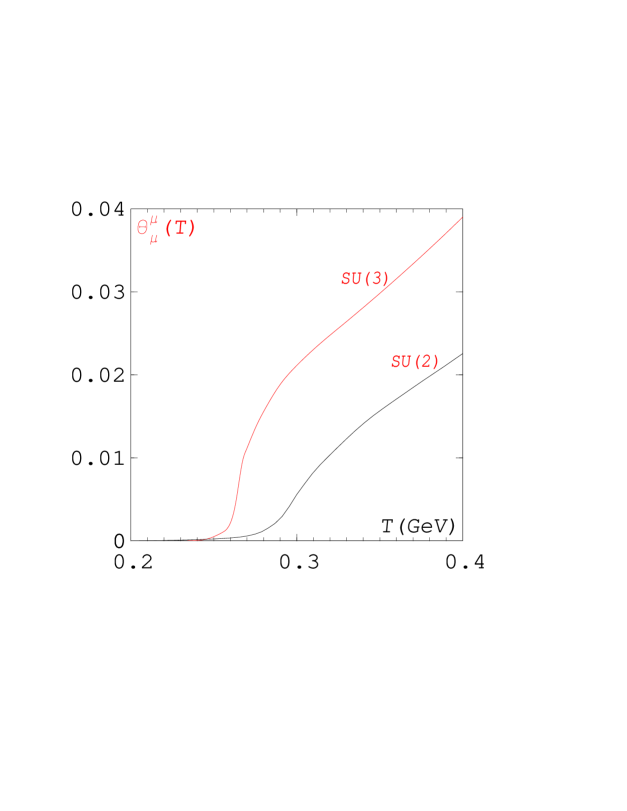
Figure 1: We compare the computed values of trace of the energy momentum tensor in the units $[GeV^{4}]$ for the lattice gauge theories $SU(2)$ and $SU(3)$ as indicated. The values for the deconfinement temperature are $T_{d}=0.290,0.264$ GeV for $SU(2)$ and $SU(3)$, respectively.

There are no other contributions to this trace for the pure gauge fields on the lattice. The heat conductivity is zero. Since there are no other finite conserved quantum numbers and, as well, no velocity gradient in the lattice computations, hence no contributions from the viscosity terms appear. For a scale invariant system, such as a gas of free massless particles, then the trace of the energy momentum tensor in equation (16) is clearly zero. However, any system that is scale variant, perhaps from a particle mass, has a finite trace, whereby the value of the trace then measures the magnitude of scale breaking. These results are shown in figure 1.
 
We now discuss a few other important properties of the pure gauge theories on the lattice. The order parameter is often taken as the lattice average of the Polyakov loop [3] , which in many cases turns out to give more information as the order parameter than does the general Wilson loop. The defining operator for the Polyakov loop is given by

$$L(\vec{x})={{1}\over{3}}{\prod}^{N_{\tau}}_{x_{4}=1}U_{4}(\vec{x},x_{4}),$$ (17)

where the index 4 stands for the euclidean time direction. Then the actual Polyakov loop is defined by the expectation value as

$$L={{1}\over{{N_{\sigma}}^{3}}}\langle{\sum}_{\vec{x}}L(\vec{x})\rangle.$$ (18)

Since a vanishing expectation value is generally a signal of an exact symmetry, one oftentimes defines the absolute value of the quantity $\bar{L}$ as

$$\bar{L}={{1}\over{{N_{\sigma}}^{3}}}\langle|{\sum}_{\vec{x}}L(\vec{x})|\rangle,$$ (19)

which serves as an approximate order parameter. For the pure gauge theories one can determine the critical couplings $\beta_{c}$ from the analysis of the Polyakov loop susceptibility $\chi_{L}$,

$${{\chi}_{L}}~{}=~{}N^{3}_{\sigma}{\left[\langle L^{2}\rangle~{}-~{}{\langle L\rangle}^{2}\right]},$$ (20)

which we shall later discuss in more detail in conjunction with the dynamical quarks in the next section. From this calculation one can accurately determine the value of the deconfinement temperature $T_{d}$.
 
 
II.2 Thermal Field Theoretical Evaluation
 
In a very recent work Zwanziger [53] has carried out an analytical determination of the properties of the equation of state for the pure gluon plasma at high temperatures well above the deconfinement temperatures. He uses the Gribov dispersion relation [54] as a means of suppressing the infrared modes when gauge equivalence is imposed at the nonperturbative level, which takes the form

$$E(k)~{}=~{}\sqrt{k^{2}+M^{4}/k^{2}}.$$ (21)

After a brief analysis of the trace anomaly at finite temperature [28] as well as comparison with the $SU(3)$ lattice data [10] Zwanziger derives a form of the trace of the energy momentum tensor

$$\theta^{\mu}_{\mu}(T)=LT~{}+~{}A,$$ (22)

where $A$ is a temperature independent term of order $O\left(1\right)$ in the units $[GeV^{4}]$ and $L$ is an integral of the form [53]

$$L~{}=~{}{{3({{N^{2}}_{c}}-1)}/{\pi^{2}}}{\int^{\infty}_{0}}dkk^{2}\ln[{{E(k)}/{k}}],$$ (23)

This integral can be exactly evaluated for the Gribov dispersion relation (21) yielding the following result:

$$L~{}=~{}{{(N^{2}_{c}-1)M^{3}}/{\pi\sqrt{2}}}.$$ (24)

Although this result with a linear growth in the temperature for $\theta^{\mu}_{\mu}(T)$ had been already observed [37, 52] in the lattice data, it had not been previously derived analytically for this energy spectrum [53]. If one looks carefully at the figure 1 for $\theta^{\mu}_{\mu}(T)$, one sees well above the deconfinement temperatures $T_{d}$ that both the curves begin to slow up to an almost linear behavior as a function of temperature T even for the temperatures of around $2T_{d}$. Nevertheless, there still are some quite gradual changes of curvature upwards until almost $3T_{d}$ or about $T=0.8GeV$, whereupon, it appears for higher temperatures to be quite linear [37]. Furthermore, one sees a new scale $M$ in the equation (21) which has the units $[GeV]$. According to Zwanziger [53] it arises from the infrared regulator, which can be estimated to be around $0.7GeV$. From a more general standpoint what is very interesting about Zwanziger’s analytical calculation of $\theta^{\mu}_{\mu}(T)$ is that the linear result for the temperature arises from the regulation of the infrared behavior of QCD which dominates over this high temperature domain. It is by now very well known that there are serious infrared problems in the high temperature perturbation theory [55], which are not easily dealt with using the standard perturbation theory. These problems indicate that the asymptotic freedom may only be strictly valid in the region of short distances and times [3]. We already know that for QCD the asymptotic freedom has appeared in the beta function as a property of the ultraviolet structure. This property of QCD provides a stable ultraviolet fixed point in the beta function in contrast to quantum electrodynamics (QED) which has a stable infrared fixed point [56, 20, 57]. However, this fact means that QED is infrared stable in contrast to QCD.
 
II.3 Numerical Evaluations of Physical Quantities
 
The numerical evaluation of the equation of state at finite temperature for strongly interacting quarks and gluons has long been the main objective for lattice simulations [2, 3, 5]. The computed pressure ratio $p(T)/T^{4}$ for the pure SU(3) lattice gauge theory [10] is shown as a function of temperature in their Figure 4 with three different values of $N_{\tau}$ in the Euclidean time direction. They remark concerning the sizes of the lattices for the different cases ${N_{\sigma}}^{3}\times{N_{\tau}}$. In what follows we take the spatial sizes ${N_{\sigma}}a$ and temporal sizes $N_{\tau}a$ whereby $a$ is the lattice spacing between points on the lattice. In these particular computations [10] the spatial step numbers have the two values ${N_{\sigma}}=16,32$ while the temporal number have the three values $N_{\tau}=4,6,8$, each of which has been explicitly studied [10]. We should note that in their Figure 4 the value for the ”critical” deconfinement temperature called $T_{c}$ for the different lattice sizes has been been evaluated from the renormalization group beta function on the lattice. The attained value for $T_{c}$ from an extrapolation to the continuum limit is given by $T_{c}/\sqrt{\sigma}=0.629(3)$. The string tension is taken for their simulations as $\sqrt{\sigma}=420MeV$, which results in a ”critical” temperature of about $T_{c}=264MeV$.
 
The actual simulations [8] for the pressure ratio in $SU(N_{c})$ around $T_{c}$ was proposed by using the integral method, which prevented the undesirable effects in some earlier evaluations of the pressure, in which the pressure ratio appeared to be negative near the critical coupling [58, 59]. Furthermore, the computational effect of the lattice anisotropy can be very accurately computed by using the integral and differential methods for the anisotropy coefficients leading to a much higher resolution. This program has been discussed in detail more recently [39] by showing how these lattice computations for both $SU(2)$ and $SU(3)$ are carried out. Similarly the energy density $\varepsilon(T)$ is calculated from the pressure $p$ and the interaction measure $\Delta(T)$ to arrive at the form $\Delta(T){\cdot}T^{4}~{}+~{}3p$ as a function of temperature. This method was briefly mentioned earlier. These numerical results are shown in a similar plot in their Figure 6 with the same basic parameters as those for the pressure ratio [10]. In their Figure 6 we can see that the energy density ratio $\varepsilon(T)/T^{4}$ as a function of the temperature $T$ for pure $SU(3)$ gauge theory rises much faster around the critical temperature $T_{c}$ than does the pressure ratio $p(T)/T^{4}$ in the previously mentioned Figure 4. It is evaluated from the interaction measure as a function of the coupling. In the sense of the thermodynamics the internal energy is generally used to thermally describe the state of the system. Thus we may well expect that its derived form as a density, $\varepsilon(T)$, should be more sensitive to the change of phase at $T_{c}$. From a casual view of the number scale we are able to see that the energy density ratio curves in each case for $N_{\tau}$ always lie considerably above that of the pressure– even above three times the corresponding numerical values [10].
 
Now we look explicitly at the equation of state of the pure gauge theory which is gotten directly from $\Delta(T){\cdot}T^{4}$. Thus this quantity which we have discussed extensively in the Introduction is simply related to the trace of the energy momentum tensor $\theta^{\mu}_{\mu}(T)$ given above in the equation (2). Here we plot the equation of state $\varepsilon-3p$ as a function of $T/T_{c}$.

Figure 2: The equation of state $\varepsilon-3p$ for pure SU(3) gauge theory with the three lattice sizes in the physical units $[GeV^{4}]$. The temperature is given as $T/T_{c}$.

Furthermore, we want to point out carefully the continual growth of the equation of state for pure $SU(3)$ gauge theory as shown in the Figure 2. This fact arising from these numerical simulations shows a behavior that is quite contrary to many of the common speculations on the equation of state for the quark-gluon plasma. We can see here no obvious signs from any of these computations that the dependence of this quantity $\varepsilon(T)-3p(T)$ decreases to zero at any temperature above the ”critical” deconfinement temperature $T_{c}$. In fact, one can reaffirm here with only very minor variations for the sizes of the different finite lattices that the high temperature linear $T$ dependence theoretically calculated [53] is still quite well upheld. Thus it is safe to conclude that the pure $SU(3)$ gauge theory in the computed range of temperatures remains a strongly interacting system of gluons– not an ideal ultrarelativistic gas!
 
 
II.4 Comparison of the Physical Quantities
 
In this paragraph the results of all these computations are summarized in the last figure in this part. In this Figure  3 we make an actual comparison using the physical units which are written below the curves in the square brackets. Here we can clearly see the differences between these computed thermodynamical quantities as functions [10] of the temperature $T[MeV]$. In addition to the above analysed quantities we have included the entropy density $s[fm^{-3}]$ which is obtained from $(\varepsilon+p)/T$, all of which are known. However, the entropy density $s[fm^{-3}]$ shown as the upper curve on the right cannot be directly compared with the others because of the units. The equation of state $\varepsilon-3p[GeV/fm^{3}]$ as the lower curve on the right can be compared with the energy density $\varepsilon$ and the pressure $p$, since all are in the same units. One can see that for these physical quantities the relative growth of each at the deconfinement temperature $T_{d}$. Above $T_{d}$ each one flattens out at different rates. This effect we can clearly see in the comparison for pure gauge theory in Figure 3. The growth of the equation of state is obviously very much slower than all the other thermodynamical quantities. This difference amounts to the comparison of a linear increase in the temperature to those with cubic or quartic powers when taken on a logarithmic scale.

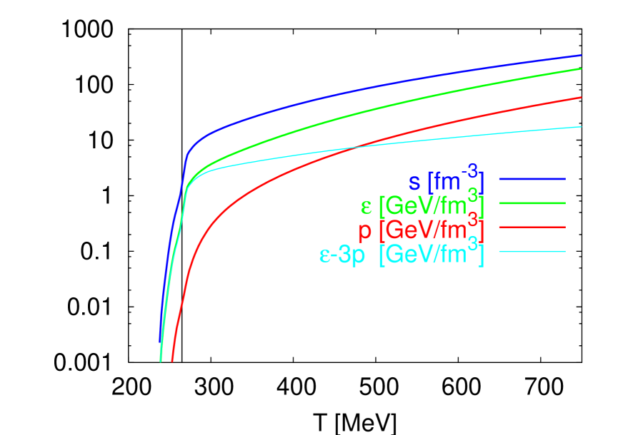
Figure 3: The different thermodynamical functions of the temperature for pure gauge theory. The vertical line is the deconfinement temperature. Here we take for these comparisons the more useful density units rather than the pure energy units as in the previous figures.

There has been some recent high temperture work in perturbation theory [61] to higher orders in the coupling $g$, for which the pressure ratio to the Stefan-Boltzmann limit has been compared to the lattice results for the pure gauge theory [10]. Furthermore, a comparison between the perturbative results [62] up to the order $O\left(g^{6}\right)$ and these lattice gauge simulations in Figure 2 for $\varepsilon-3p$ shows a very good agreement above about $800MeV$. This perturbative evaluation for $\varepsilon-3p$ continues to increase well beyond the range of the lattice data in roughly the same way as the simulations [10].
 
II.5 Discussion of Conformal Symmetry
 
Specific investigations of the effective measure of conformal symmetry have been recently carried out on the lattice at high temperatures for pure $SU(3)$ gauge theory. As we have already discussed above in the Introduction, the presence of a nonzero trace for the energy momentum tensor relates with the breaking of scale and conformal invariance. We shall discuss more thoroughly in the Appendix B the mathematical nature of the related physical currents $D^{\mu}(x)$ and $K^{\mu\alpha}(x)$ which are relate directly to the fact that the trace of the energy momentum tensor remains finite.
 
Then the question clearly arises concerning how close the given thermodynamical system is to achieving the scale and conformal invariances. A measure of the deviation from conformality is given by the expression $\mathcal{C}=(\varepsilon-3p)/{\varepsilon}$, which has been proposed by Rajiv Gavai, Sourendu Gupta and Swagato Mukherjee [60]. Clearly if the value of $\mathcal{C}$ were identically zero, then the conformal invariance of the theory would be fully upheld. However, they clearly find from their simulations [60] at both the temperatures of $2T_{d}$ and $3T_{d}$ the regions with finite (nonzero) values for $\mathcal{C}$. Thereby they show in a plot of the pressure ratio $p/T^{4}$ against the energy density ratio ${\varepsilon}/T^{4}$ that all the numbers lie significantly below the line of conformality in the pressure where $\mathcal{C}=0$, which corresponds to the ideal ultrarelativistic gas. Then from their work we are able to see that all of the values of $p/T^{4}$ and ${\varepsilon}/T^{4}$ in their simulations are visibly removed from their ideal gas values for a lattice with those given quantum numbers of the spin and color. Thus for pure gluon system we would expect to find the Stefan-Boltzmann limiting values for these ratios to be $8\pi^{2}/45$ and $8\pi^{2}/15$, respectively. Furthermore, the higher temperature points at $3T_{d}$ are distributed in a cluster which appears to be further from the line of conformality $\mathcal{C}=0$ than were those at $2T_{d}$.
 
Finally we conclude this part on the thermodynamics of the pure lattice gauge theory. In summary, for the gluon gas with strong interactions simulated for both $SU(2)$ and $SU(3)$ symmetries all the thermodynamical functions in physical units including the equation of state grow monotonically in the temperature. This clear statement from the computed numerical results is obviously quite contrary to the usual expectations from the ideal gas oriented theories. In some earlier investigations and collaboration with Graham Boyd [37, 52] we have shown further properties of these thermodynamical functions to possess a steady growth in the presently considered range of temperatures continuing to, at least, $1.5[GeV]$.
 

III. Dynamical Quarks at finite Temperature
 
In this part of the report we look at the full lattice QCD including the thermodynamical contributions to the equation of state arising from the thermal properties of the dynamical quarks. The presence of these quarks with multiple flavors changes radically the evaluation of the thermodynamical quantities. The changes are largely due to the presence of the broken chiral symmetry in the hadronic ground state of the colored quark fields. Furthermore, the restoration of the chiral symmetry at finite temperatures radically restructures the high temperature quark-gluon phases. The critical temperature $T_{c}$ for the chiral restoration is considerably lower than the deconfinement temperature $T_{d}$ for the pure $SU(N_{c})$ lattice gauge theories discussed in the last section. The order parameter can be defined similarly to the Polyakov loop $L$ in equation (18) for the pure gauge theory except that one takes only the real part $\Re{e~{}L}$ when the dynamical quarks are present [68, 69].
 
Before we consider the actual lattice data, we mention the thermodynamics of the ideal relativistic gas of $n_{f}$ flavored quarks with a given rest mass $m$ at a temperature $T$. The quantities like the pressure and the energy density are well known, which gives the equation of state

$$\varepsilon(T)-3p(T)=g{m^{3}}T{K_{1}(m/T)},$$ (25)

where $K_{1}(m/T)$ is the modified Bessel function of the second kind. The statistical degeneracy factor $g$ has the value $3n_{f}/{\pi}^{2}$. For a fixed quark mass $m$ and at temperatures large compared to the mass energy then the right side of (25) becomes just $g{m^{2}}{T^{2}}$. Then the equation of state of a pure massive gas grows quadratically in both the temperature and the mass in the high temperature limit.
 
III.1 Equation of State for two light Quark Flavors
 
First we consider the equation of state for two light dynamical quarks which appears as a plot similar to the figure 2 for the pure $SU(N_{c})$ gauge theories in terms of the trace of the energy momentum tensor for the equation of state ${\theta}^{\mu}_{\mu}(T)~{}=~{}\epsilon(T)~{}-~{}3p$. In this new figure for the MILC97 data [50] we have shown the equation of state using equation (16) in terms of the physical units $[GeV/fm^{3}]$.

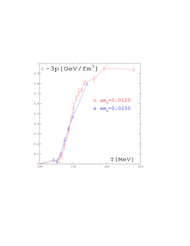
Figure 4: The equation of state for two light quarks given by the two different lattice masses.

Furthermore, in this representation we are able to compare our results directly with those in their Figure 7 for the MILC data [50] which shows the interaction measure written as $(\varepsilon-3p)/T^{4}$ against the QCD lattice coupling $6/g^{2}$ over the range of values from 5.36 to 5.50 with the two mass values $am_{q}=0.0125$ and $am_{q}=0.0250$, which are expressed in terms of the lattice spacing.
 
It is important that we note here for the case of the light dynamical fermions that even though the pressure ratio is computed in a similar way to the pure lattice gauge theory starting with the equation (10), it, nevertheless, has the predominant effect of the average of the product of the antiquark $\bar{\psi}_{q}$ and quark $\psi_{q}$ fields written as ${\langle\bar{\psi}_{q}{\psi}_{q}\rangle}$. Thus the equation for the pressure ratio (13) gets modified to contain these contributions. Since we do not present here the numerical values for the pressure, one should go to the original MILC97 data [50] for the exact form of the pressure equation, which, however, uses slightly different notation in the integration method as applied to the free energy ratio. For this reason the interaction measure has an additional contribution beyond just the plaquette terms of the pure lattice gauge theory as given in equation (15). This new term arises from the mass renormalization on the antiquark-quark terms ${\langle\bar{\psi}_{q}{\psi}_{q}\rangle}$. These two contributions together give the interaction measure $\Delta_{m}(T)$ with the the quarks of mass $m_{q}$

$$\Delta_{m}(T)={n^{4}_{\tau}}~{}\{{\tilde{\beta}(g)}~{}{\left[S_{0}~{}-~{}S_{T}\right]}~{}+~{}\tilde{\gamma}(am_{q})\left[{\langle\bar{\psi}_{q}{\psi}_{q}\rangle}_{0}~{}-~{}{\langle\bar{\psi}_{q}{\psi}_{q}\rangle}\right]\}.$$ (26)

The beta function ${\tilde{\beta}(g)}$ is given similarly to that in equation (14).However, the renormalization group gamma function for QCD [56] can be defined on the lattice $~{}\tilde{\gamma}(am_{q})$ as

$${\tilde{\gamma}(am_{q})}~{}=~{}-{\frac{d(am_{q})}{da}}.$$ (27)

The presence of both these terms in $\Delta_{m}(T)$ carries very important consequences in the equation of state as can be seen in the figure 4. The behavior between around $100MeV$ up to just below $250MeV$ for the MILC97 data [50], that is near to and just above $T_{c}$ shows a decisively different change in the equation of state from that of the pure $SU(3)$ gauge theory just above $T_{d}$ as seen in figure 2. Although the pure gauge theory shows some variation in its rise above $T_{d}$ depending upon the lattice sizes [10], after about $300MeV$ its increase is reduced to an approximately linear rate [53]. In the later paragraphs we shall contrast both these results with some newer lattice computations for different numbers and masses of quarks. First, however, we shall discuss a little more carefully the structure of chiral symmetry breaking.

III.2 Chiral Symmetry and Dynamical Quarks
 
In the presence of dynamical quarks another symmetry becomes important– the chiral symmetry. When the quarks have masses, this symmetry is automatically broken. The chiral symmetry is a property of the two different representations of $SL(2,\bf{C})$ denoted by $\bf{2}$ and $\bf{2^{*}}$ arising for the Dirac spinors in the Weyl representation [20]. It is the presence of the quarks’ mass terms in the Dirac equation that formally breaks the chiral symmetry. This comes formally out of the nonconservation of the axial current $j^{\mu}_{5}$ as discussed [35, 20] relating to the triangle diagrams, such that the chiral anomaly for QCD takes the form

$$\partial_{\mu}j^{\mu}_{5}~{}=~{}j_{5}~{}+{{k_{1}}\over{8\pi^{2}}}{{\bar{G}^{\mu\nu}_{a}}G^{a}_{\mu\nu}},$$ (28)

where $k_{1}$ is a constant and $j_{5}$ is a pseudoscalar contribution. This situation has important implications in the case for finite temperatures where for $T$ sufficiently high the chiral symmetry is restored in the small mass or chiral limit, $m_{q}\rightarrow 0$. We shall discuss the implications of this both from the theoretical side and the numerical side where a finite small mass is present.
 
We now look at the chiral condensate at finite temperatures using chiral perturbation theory. The low temperature expansion for two massless quarks can be written [28] in the following form:

$${{\langle\bar{\psi}_{q}{\psi}_{q}\rangle_{T}}\over{\langle\bar{\psi}_{q}{\psi}_{q}\rangle}_{0}}~{}=~{}1~{}-~{}{1\over{8}}{T^{2}\over{F^{2}_{\pi}}}~{}-~{}{1\over{384}}{T^{4}\over{F^{4}_{\pi}}}~{}-~{}{1\over{288}}{T^{6}\over{F^{6}_{\pi}}}{\left\{ln{{\Lambda_{q}}\over{T}}\right\}}~{}+~{}O(T^{8})~{}+~{}O(\exp{-M\over{T}}),$$ (29)

where $F_{\pi}$ is the above mentioned pion decay constant and the scale $\Lambda_{q}$ is taken as approxamately $0.470GeV$. Leutwyler has shown that this expansion up to three loops remains very good at least up to around $0.100GeV$. At very low temperatures the probability of finding any given excited mass state is related to the exponentially small correction, which in this case has a very small value. As the temperature becomes higher, the number of different states begins to grow . Nevertheless, at sufficiently low temperatures the excited states may be regarded as a dilute gas of free particles since the chiral symmetry supresses the interactions by a power of $T$ of this gas of excited states with the primary pionic component [28].
 
Upon approaching the chiral symmetry restoration temperature $T_{\chi}$ the picture changes drastically. At this point the ratio $T/F_{\pi}$ is considerably greater than unity. It is here where one expects the chiral condensate to be very small or to have totally to have vanished. This effect has been studied recently numerically  [40] for two light flavors at finite temperature on the lattice. The results of this simulation is shown for ${{\langle\bar{\psi}_{q}{\psi}_{q}\rangle_{T}}/{\langle\bar{\psi}_{q}{\psi}_{q}\rangle}_{0}}$, which we simply write as the quark condensate ratio, $\langle\bar{\psi}{\psi}\rangle$, in the following two plots for the restoration of chiral symmetry. We show this quark condensate ratio as a function of the coupling $\beta$ for the range where the chiral symmetry is mostly restored [40]. The Figure 5 shows this ratio for two light quarks with a mass in lattice units of $0.02$ on a lattice of size $16^{3}\times 4$. We remark that at the value for the coupling 5.24 the chiral symmetry for the two light quarks with the lattice mass of 0.02 is already about $20\%$ restored. While at the upper value of 5.33 it is still only about $80\%$ restored. Thus we see that the chiral limit has not in this case been reached.

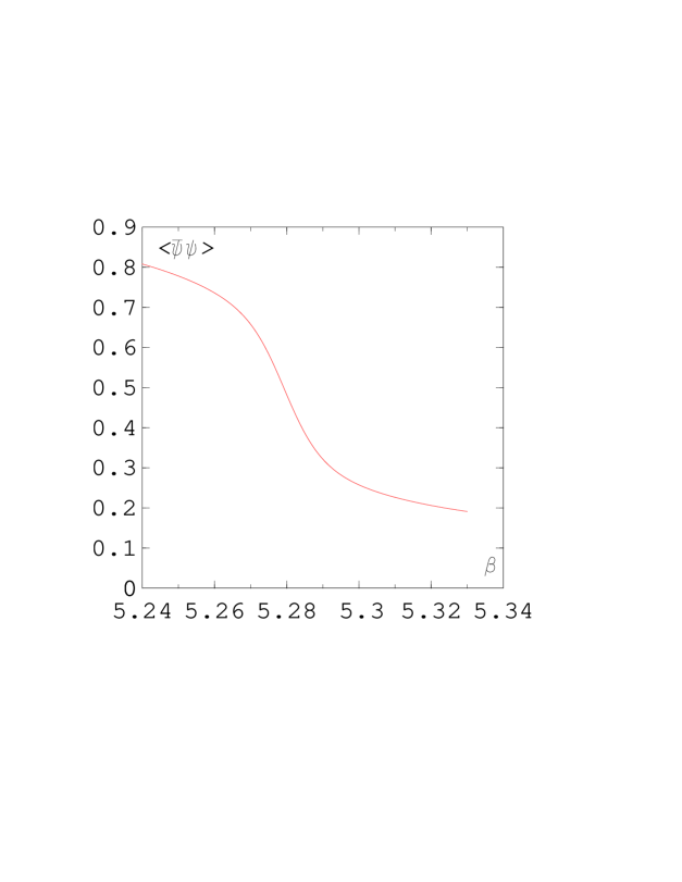
Figure 5: We show $<\bar{\psi}\psi>$ as a function of the coupling $\beta$ for the quark mass in lattice units $ma$= 0.02, which is normalized to the vacuum value of the chiral condensate.

The Figure 6 comparess how the different mass values shown from left to right of $0.02$, $0.0375$ and $0.075$ depend upon the given lattice sizes, which are $8^{3}\times 4$, $12^{3}\times 4$ and $16^{3}\times 4$.

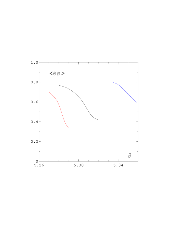
Figure 6: We show the same physical quantity with the different values of the quark masses 0.02, 0.0375 and 0.075 from left to right [40].

We should also notice how the larger mass values slow the restoration down, which corresponds to moving the transition $T_{\chi}$ to higher temperatures or even eliminating it altogether as indicated by the flatness of the curves.
 
III.3 Thermodynamics with Dynamical Quarks
 
The main quantities which were analyzed here were the various susceptibilities:  
1. The Polyakov loop susceptibility we have defined earlier in the last section in the equation (20). We will use now in connection with two other forms of the susceptibilities which are to follow:
 
2. The magnetic or chiral susceptibility;

$${{\chi}_{m}}~{}=~{}{T\over V}~{}{\sum\limits_{i=1}^{n_{f}}}{{\partial^{2}}\over{\partial m^{2}_{i}}}{\ln{\cal{Z}(T,V)}},$$ (30)

3. The thermal susceptibility;

$${{\chi}_{\theta}}~{}=~{}-{T\over V}~{}{\sum\limits_{i=1}^{n_{f}}}{{\partial^{2}}\over{\partial m_{i}\partial(1/T)}}{\ln{\cal{Z}(T,V)}}.$$ (31)

One compares the critical properties of ${{\chi}_{L}}$, ${{\chi}_{m}}$ and ${{\chi}_{\theta}}$ in order to establish the value of $T_{\chi}$ and its critical properties in the chiral limit where $m_{q}\rightarrow 0$. For the moment we use $T_{\chi}$ for the chiral restoration temperature in contrast to the critical temperature $T_{c}$ for the dynamical quark simulations. However, in numerical simulations $m_{i}$ must be taken to be finite– this means that one must use various different small values of $m_{i}$ on the different sized lattices $N^{3}_{\sigma}\times N_{\tau}$. This procedure uses the lattice data to find the values around the peak of the susceptibility ${{\chi}_{m}}$ at $T_{\chi}$ for the smallest masses, with which one can determine the critical structure. A careful determination of the topological susceptibility relating to the chiral current correlations can be related to the square of the topological charge $Q^{2}_{T}$ in the chiral limit [41], such that

$${n_{f}\over{m}}\langle Q^{2}_{T}\rangle~{}=~{}V{\langle\bar{\psi}{\psi}\rangle}_{m\rightarrow 0},$$ (32)

where $n_{f}$ is the number of flavors. Thus from these susceptibilities one can arrive at the quark condensate ratio $\langle\bar{\psi}{\psi}\rangle$. However, in this computation it is a major problem to properly set the temperature scale for small lattices with finite masses. The plots in the figure 5 and 6 are made with the coupling $\beta$ which may be compared with pure $SU(3)$ on one side and the two flavor dynamical quark simulations on the other [50]. In the case of pure $SU(3)$ the critical coupling $\beta_{c}$ for a ${16^{3}}\times 4$ lattice has the value [10] of about 5.70, which is considerably larger than the values of $\beta$ shown in the figure 5 and  6. However, for the two light flavored dynamical quarks [50] the value of ${\beta}_{c}$ is around 5.40, which is still somewhat above these values shown in the two figures.
 
Here we have investigated the properties of the chiral symmetry restoration for the quark condensate $\langle\bar{\psi}_{q}{\psi}_{q}\rangle$ alone at various values of the coupling $\beta$. We have also shown in the figure 6 how the coupling shifts to higher numbers for larger values of the mass. These results can be compared to the MILC97 data [50] with much lighter quark masses which, nevertheless, stays mostly in the same range of the couplings (see in the reference  [50] their figure 4.) We can see there that this data is extended into a higher range of coupling to get considerably smaller values of the quark condensate. These values we shall use in the next section for the mass contribution of the quark condensate at higher values of the temperature. We can then compare this effect in the chiral limit. However, here it is very difficult to immediately go over to a physical temperature scale in the same way as in the previous section for the pure gauge or gluon system. In what follows we shall look into the gluon condensate in the presence of dynamical quarks. Here we know that the presence of the quark masses are an immediate cause of scale symmetry breaking which of course change the scale of the system. This in turn changes the beta function as well as adds a term due to the mass renormalization. Thus the renormalization group equations are changed accordingly. This effect we shall discuss more thoroughly in the following.
 
III.4 Equation of State with Different Quark Flavors
 
Next we look at the thermodynamical functions including the pressure $p(T)$, energy density $\varepsilon(T)$ and the equation of state $\varepsilon(T)-3p(T)$ all in the physical units $[GeV/fm^{3}]$ for the case of somewhat heavier dynamical quarks with different numbers and types of flavors. These different cases have been worked out in the doctoral thesis of Andreas Peikert [72] at the Universität Bielefeld for the lattices of sizes $8^{3}\times 4$, $16^{3}\times 4$ and for comparison the symmetrical lattice $16^{4}$. In general throughout these numerical simulations the masses of the different quarks were considerably heavier than the MILC97 data [50], which were taken between $7.5MeV\leq m_{q}\leq 15MeV$ . The lighter quarks had masses in these newer simulations with the values between $40MeV\leq m_{q}\leq 60MeV$, while the heavier one was more in the range of $100MeV\leq m_{q}\leq 150MeV$, which are considerably higher than the light up and down quarks, but are not so far off for the strange quarks. The presented data was simulated using the p4 action for which comparisons were made to the more usual actions [72].The resulting figures taken from these simulations we shall contrast the various different arrangements of flavors $n_{f}=2$, $n_{f}=2+1$ and $n_{f}=3$ given as functions of the temperature. In each of these flavor arrangements the quarks are at least an order of magnitude heavier than those in the previous figure 4 for the MILC97 data [50].
 

Figure 7: The pressure for the three values of $n_{f}=2,2+1,3$ with massive dynamical quarks.

We now look into the properties of each thermodynamical quantity more specifically. The Figure 7 shows the pressure $p(T)$ for the three different flavors [70, 71, 72] in a way similar to that of the pure $SU(3)$ gauge theory. Although the general shape of these curves are quite similar in appearance, the values of the temperatures for the transitions are noticably lower in the theory with the dynamical fermions. Again the pressure was computed in the same manner as that of the pure lattice $SU(N_{c})$ using the integration method [8, 9, 10] as was discussed in the last part. In the case of the pressure $p(T)[GeV/fm^{3}]$ the shape of all three curves is almost the same except for the starting point for the case of $n_{f}=2$. This is because of the difference in the value of $T_{c}$. For the case of $n_{f}=2$ the value of $T_{c}=175MeV$ is somewhat higher than $n_{f}=2+1$ and $n_{f}=3$ of around $155MeV$. However, when one plots the pressure ratio $p/T^{4}$, as was originally done [70, 71, 72], one notices a large difference in the different curves arising from the different number of degrees of freedom in each case, which changes the rate of approaching the Stefan-Boltzmann limit as well as the actual value of number itself. In our figure 7 the pressure in physical units represented on a logarithmetrical scale appear to start very near to the actual value of $T_{c}$. However, in the form of the ratio $p/T^{4}$ the small values for the different flavors start well below $T_{c}$ with a very gradual increase until reaching the critical temperature. Thereabove the increase in each curve is at different rates due to the different number of degrees of freedom and the corresponding masses. In the actual original plot [72] (see figure 4.8) of $p/T^{4}$ against $T/T_{c}$, one sees that the curve for $n_{f}=2$ lies well under that of $n_{f}=2+1$, which itself is significantly under that of the cases of $n_{f}=3$. Furthermore, the placing of these curves is quite different on the approach to the Stefan-Boltzmann limit. At the temperature of about $4T_{c}$ the case of $n_{f}=2+1$ has only achieved around $75\%$, whereas both the cases $n_{f}=2$ and $n_{f}=3$ have arrived at about $80\%$ of their respective limiting values for high temperatures. Whether this limiting value is actually attained in the high temperature limit, still remains as an open question. Finally we remark that in the case of the pressure the errorbars are generally very small so that their presence is not essential to the figure.
 

Figure 8: The energy density for the three values of $n_{f}=2,2+1,3$ with massive dynamical quarks.

We next turn our attention to the energy density $\varepsilon(T)$ which presents quite a different problemmatic in the computation. The corresponding accuracy of the evaluations is considerably lower, which may be apparent by the presence of the errorbars in figure 8. There we see that $\varepsilon(T)[GeV/fm^{3}]$ shows a quite different behavior as a function of the temperature $T[MeV]$ from that of the pressure in the Figure 7. Even well below $T_{c}$ there are small values of $\varepsilon(T)$ which then grow much more rapidly at $T_{c}$. In contrast the pressure really starts to take on sizable values only at temperatures very near to $T_{c}$. Furthermore, one can see quite different rate of rise in $\varepsilon(T)$ depending upon the masses and the number of flavors. Nevertheless, its values start off at lower temperatures and rise more slowly than the corresponding values of $p$. Then just above $T_{c}$ the energy density $\varepsilon(T)$ rises very rapidly as a function of $T[MeV]$. We notice that the curve for $n_{f}=2$ starts later because of the larger $T_{c}$ and rises more slowly just above $T_{c}$. For temperatures above about $200MeV$ $\varepsilon(T)$ for all the three flavors rise at approximately the same rate–practically on top of eachother. However, the $n_{f}=2$ the values always remain somewhat below the others as it was also the case for the pressure curves.

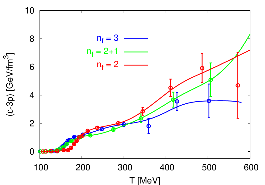
Figure 9: The equation of state is evaluated for the three values of $n_{f}=2,2+1,3$ including the massive dynamical quarks.

From the knowledge of the pressure $p(T)$ as well as the energy density $\varepsilon(T)$ we are able to calculate the equation of state in terms of $\varepsilon(T)-3p(T)$. However, even as a difference between these basic physical quantities the equation of state still shows another type of behavior in relation to the flavors $n_{f}$ and the quark masses $m_{q}$. The values of the masses in the stated ranges have always held the $n_{f}=2$ values of these thermodynamical functions of the temperature to be smaller than $n_{f}=2+1$ and $n_{f}=3$. However, we see in figure 9 that this statement holds only up to about $200MeV$, above which temperature the $n_{f}=2$ values remain within the errorbars clearly larger than the others. Furthermore, above about $300MeV$ the case with $n_{f}=2+1$ takes on larger values than $n_{f}=3$, but still remains smaller than $n_{f}=2$. Furthermore, in this range between $200MeV$ and $300MeV$ the change is very slow when compared with the region between $150MeV$ and $200MeV$ near the critical points. Thus we can clearly see here the types of contrasts between the parameters and the physical quantities. We remark also that for the equation of state the problem with the error bars at higher temperatures becomes very significant so that in all cases above $500MeV$ the curves give no real physical predictions.
 
In this section we have numerically evaluated using the lattice gauge simulations [70, 71, 72]. We have shown the thermal properties in the three separate figures 7,8 and  9 the basic thermodynamical quantities– the pressure $p(T)$, the energy density $\varepsilon(T)$ and the equation of state in the form $\varepsilon(T)-3p(T)$ as functions of the temperature $T$. Furthermore, we have looked at these quantities in terms of the input parameters like the number of quark flavors and the quark masses, for which earlier in this part we have brought in the properties of chiral symmetry through the chiral condensate ratio. In the next section we shall briefly discuss some very recent data appearing within the last year, which we can compare with the above shown results for different values of the lattice mass parameters.
 
 
III.5 Discussion of Recent Massive Quark Data
 
Since the start of the actual writing of this work, there have appeared some newer data [73, 74] for the three quark equation of state. In this section we shall present a discussion of some of these newer numerical simulations for 2+1 flavors with a brief analysis of the lattice results. In particular, we look at the simulations [74] plotted as a function of the ratio $T/T_{c}$ in their Figure 1, in which they include the data points for the following lattice quantities: the interaction measure, here written as $I/T^{4}$, the pressure ratio $p/T^{4}$ and the energy density ratio $\varepsilon/T^{4}$. In their simulations they use a Symanzik improved gauge action and the Asqtad $O(a^{2})$ improved staggered quark action for lattices with the temporal extents $N_{\tau}=4$ and $N_{\tau}=6$. They set their value of the heavy quark mass near to the physical strange quark mass $m_{s}$. Then they choose the two degenerate light quark masses to have the values of $0.1m_{s}$ and $0.2m_{s}$, for which they compute these quantities in the temperature range from $0.7T_{c}$ to $2.15T_{c}$. For the computation of these thermodynamical ratios the integral method [8] has been used as discussed in previous sections. Furthermore, the estimated value [73] of the critical temperature $T_{c}$ is somewhat higher than for the Bielefeld 2+1 flavor data for this system with much lighter quarks, which is found to be about $169\pm 12\pm 4MeV$.
 
These more recent results may be properly compared to the Bielefeld data [70, 71, 72] only for the simulations with $N_{\tau}=4$. In general we can compare the values for the interaction measure in the 2+1 flavor case [72] used in the above figure 9 to compute the equation of state to those values of $I/T^{4}$ plotted for $N_{\tau}=4$ in the Figure 1 of this newer work [74]. This comparison shows that the actual difference between the does not result in a large change in the interaction measure. Therefore, we could expect to have rather small changes in the properties of the equation of state over the temperature range in common to both cases. A simple pointwise comparison shows that for temperatures below and just above $T_{c}$ the values for the interaction measures are close to the same for both cases within the respective errorbars. Above $1.5T_{c}$ the newer values of the interaction measure are actually somewhat larger. In the case of $N_{\tau}=6$ the numerical values for the interaction measure are considerably larger than the corresponding values for the Bielefeld data [70, 71, 72] just above $T_{c}$ and remain so throughout the higher temperatures.
 
In summary for this new data we notice that the $N_{\tau}=4$ is generally closer to the numerical values used here. The larger values for the light quark mass provide the bigger numbers for the interaction measure especially around the critical temperature. We should also mention some values for the quantity $\varepsilon/T^{4}$ approach the Stefan-Boltzmann limit for the $N_{\tau}=6$ simulations near to $1.25T_{c}$, after which the changes in value are quite small. This fact accounts for the larger growth of the interaction measure near to $T_{c}$. This new data describes the QCD thermodynamics for three flavors of improved staggered quarks quite consistently with the data use here [70, 71, 72]. In the next part we will consider the results from our previous analyses of the equations of state in the figures 4 and 9 in more detail in relation to the gluon and quark condensates at finite temperature.

IV. Gluon and Quark Condensates at Finite Temperature
 
In this part we start our discussion of the thermal properties of the gluon condensates by using the approach that we described in the Introduction which includes both the pure $SU(2)$ and $SU(3)$ gauge theories [10, 37] as well as the massive quarks [52]. We shall first discuss how the pure gluon condensate looks with no dynamical quarks present, for which the results for the equation of state in Part II can be directly used. The effects of the chiral phase transition with massive dynamical quarks are then discussed in various cases, for which we discuss the different relationships to the quark condensates.

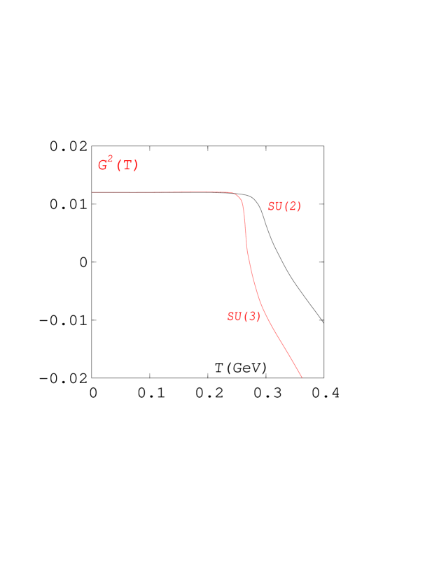
Figure 10: We show the gluon condensates for the $SU(2)$ and $SU(3)$ invariant gauge theories, where both the ordinates are in $[GeV^{4}]$.

IV.1 Pure Gluon Condensate
 
The results for the gluon condensation in the cases of the pure gauge theories are shown in the figure 10 for the lattice data [9, 10]. In both these cases we have taken the zero temperature gluon condensate [36] to be $\langle G^{2}\rangle_{0}~{}=~{}0.012[GeV^{4}]$ as the starting value for the gluon condensate at finite temperature, which we shall write for simplicity $G^{2}(T)$. We can see that this value remains very constant for temperatures up to nearly the deconfinement temperature [28, 37], which are given as $T_{d}=0.290~{}and~{}0.264$ GeV for the color $SU(2)$ and $SU(3)$, respectively. The basic equation comes from the finite temperature trace anomaly which remains much the same as the one considered above used by Leutwyler [28] except that it is applied to the pure gauge theory not massless quarks. In the course of this section we shall reconsider the values in order to include the massive quarks.
 
IV.2 The Effect of Quark Condensates
 
In the presence of massive quarks the trace of the energy-momentum tensor takes the altered form [44] from the trace anomaly as given by the equation (6) for which we recall that $m_{q}$ is the light (renormalized) quark mass and ${\psi}_{q}$, $\bar{\psi}_{q}$ represent the quark and antiquark fields respectively. In the last section we have discussed the temperature dependence of the chiral condensate in relatiion to chiral perturbation theory [28]. We recall that the second term in equation (29) is quadratic in the temperature. This term corresponds to the process of pion absorption and emission given by the matrix element ${\langle\pi|\bar{\psi}{\psi}|\pi\rangle}$. This term as well as the succeeding even powers in the expansion of ${\langle\bar{\psi}{\psi}\rangle}_{T}$ allow the chiral condensate to melt quite gradually. Furthermore, we should note that in equation (29) that all the terms subtract off the zero temperature condensate. In contrast to the multitude of processes in the chiral condensate melting, Leutwyler clearly points out [28] that such terms are absent in the pure gluonic processes since the field strength operators in the color combination given in equation (4) in the form $G^{{\mu}{\nu}}_{a}G_{{\mu}{\nu}}^{a}$ is a chiral singlet so that the corresponding single pion matrix element vanishes [28]. When one calculates the corresponding trace of the energy momentum tensor, one finds for two massless flavors

$$\theta^{\mu}_{\mu}(T)~{}=~{}{\pi^{2}\over{270}}{T^{8}\over{F^{4}_{\pi}}}{\left\{ln{{\Lambda_{p}}\over{T}}~{}-~{}{1\over 4}\right\}}~{}+~{}O(T^{10}),$$ (33)

where the logarithmic scale factor ${\Lambda_{p}}$ has the approximate value of $275MeV$ [28, 45]. Thus in the framework of chiral perturbation theory the single and double loop contributions both vanish in the gluon condensate at finite temperatures. The first actual term present in the equation (33) has the power $T^{8}$ arises from the three loop graph. The result of equation (33) can be used in Leutwyler’s equation (3) to evaluate the finite temperature color averaged gluon condensate, which was discussed [28]. In the following we shall use these averages together in a single expression, both of which are evaluated from the numerical lattice gauge simulations with massive dynamical quarks. Furthermore, we shall include with these averages the renormalization group functions $\beta(g)$ and $\gamma(g,m)$, which appear in the trace of the energy momentum tensor even in the vacuum [46, 47] from the renormalization process.  
Now we need to discuss further the changes in the computational procedure which arise from the presence of dynamical quarks with a finite mass. There have been recently a number of computations of the thermodynamical quantities in full QCD with two flavors of staggered quarks  [48, 49, 50], and with four flavors [86, 51]. We have already mentioned the problemmatic of the simulations for the dynamical quarks in the equation of state in the last section. Furthermore, we mentioned there the problem of the quark condensate in relation to the restoration of chiral symmetry. Now we bring these two aspects of dynamical fermions together. Nevertheless, we first remark that these calculations are still not as accurate as those in pure gauge theory for several reasons. The first is the prohibitive cost of obtaining statistics similar to those obtained for pure lattice gauge theory. So the error on the interaction measure is considerably larger. The second reason, which is perhaps more serious, lies in the effect of the quark masses currently simulated. They are still, in most of the cases in the present simulations relatively heavy, which unduely increases the contribution of the average quark condensate part in the interaction measure. In fact, it is known that the vacuum expectation values for very heavy quarks is proportional to the gluon condensate $G^{2}_{0}$, written in simplified notation, which in the first approximation is given by [36]

$${\langle\bar{\psi}_{q}{\psi}_{q}\rangle}_{0}~{}=~{}{-1\over{12m_{q}}}{G^{2}_{0}}.$$ (34)

Furthermore, there is an additional difficulty in setting properly the temperature scale even to the extent of rather large changes in the critical temperature have been reported in the literature depending upon the method of extraction. For two flavors of quarks the values of $T_{c}$ lie between $0.140GeV$ [50] and about $0.170GeV$  [63] which is considered presently a good estimate of the physical value for the critical temperature.
 
We are now able to write down an equation for the temperature dependence of the thermally averaged trace of the energy momentum tensor including the effects of the light quarks with a mass $m$ from $\Delta_{m}(T)$ so that

$$\theta^{\mu}_{m\mu}(T)~{}=~{}\Delta_{m}(T){\cdot}T^{4}.$$ (35)

The thermally averaged gluon condensate is computed including the light quarks in the trace anomaly using the equation (6) and the interaction measure in $\theta^{\mu}_{m\mu}(T)$ to get

$$G^{2}(T)~{}+~{}{\sum}_{q}m_{q}{\langle{\bar{\psi}_{q}{\psi}_{q}}\rangle}_{T}~{}=G^{2}_{0}~{}+~{}{\sum}_{q}m_{q}{\langle{\bar{\psi}_{q}{\psi}_{q}}\rangle}_{0}~{}-~{}{\theta}^{\mu}_{m\mu}(T),$$ (36)

It is possible to see from this equation that at very low temperatures the additional contribution to the temperature dependence of the gluon condensate from the quark condensate is rather insignificant and disappears completely at zero temperature. However, in the range where the chiral symmetry is being restored there is an additional effect from the term $\langle\bar{\psi}_{q}{\psi}_{q}\rangle_{T}$, which lowers $G^{2}(T)$. Well above $T_{c}$ after the chiral symmetry has been mostly restored the only remaining effect of the quark condensate is that of $m_{q}\langle\bar{\psi}_{q}{\psi}_{q}\rangle_{0}$. It is then known [36] how this term shifts the gluon condensate of the vacuum. Thus we may well expect  [37] that for the light quarks the temperature dependence can only be important below and near to $T_{c}$. In the case of the chiral limit  $m_{q}\rightarrow 0$ the equation (37) takes the form of Leutwyler’s equation (3) as, of course, it should because Leutwyler used two massless quarks [28]. For the smaller values of the simulated quark masses in lattice units of 0.01 to 0.02 $\langle\bar{\psi}_{q}{\psi}_{q}\rangle_{T}$ has mostly disappeared in the range where $G^{2}(T)$ differs from $\langle G^{2}\rangle_{0}$.
 
IV.3 Gluon and Quark Condensates with two light Flavors
 
In the way we mentioned above for equation (3) with the change of the pure gluon condensate to the sum of the quark contributions $\langle G^{2}\rangle~{}+~{}{\sum}_{q}m_{q}\langle{\bar{\psi}_{q}{\psi}_{q}}\rangle$. First we discuss the finite temperature gluon condensate in the ”chiral limit” $m_{q}\rightarrow 0$ as shown in the figure 11 with the two $m_{q}=0$ curves. From the MILC light quark data [50] we are able to subtract the quark condensates at finite temperatures multiplied by the two quark masses $m_{q}=7.5MeV$ and $m_{q}=15MeV$ for the two sets of lattice data. The effects of the temperature as well as the restoration of the chiral symmetry are included with the decreasing value of $m_{q}<\bar{\psi}\psi>$ with increasing temperature are gotten from the original lattice data [50]. We use for the vacuum value of $<\bar{\psi}\psi>_{0}=-(259\pm 27MeV)^{3}$ from a recent estimate [75] taken from newer MILC dynamical quark data [76]. Now we can reformulate the above equation (36) by replacing the sum over the flavors simply by the number two. The the finite temperature gluon condensate is given by

$$G^{2}(T)~{}=~{}G^{2}_{0}~{}+~{}2m_{q}\langle\bar{\psi}_{q}{\psi}_{q}\rangle_{0}\left(1~{}-~{}\langle\bar{\psi}_{q}{\psi}_{q}\rangle\right)~{}-~{}\theta^{\mu}_{m\mu}(T).$$ (37)

The ratio of the finite temperature quark condensate to its vacuum value, $\langle\bar{\psi}_{q}{\psi}_{q}\rangle_{T}/{\langle\bar{\psi}_{q}{\psi}_{q}\rangle}_{0}$, we write simply as $\langle\bar{\psi}_{q}{\psi}_{q}\rangle$, which is just the

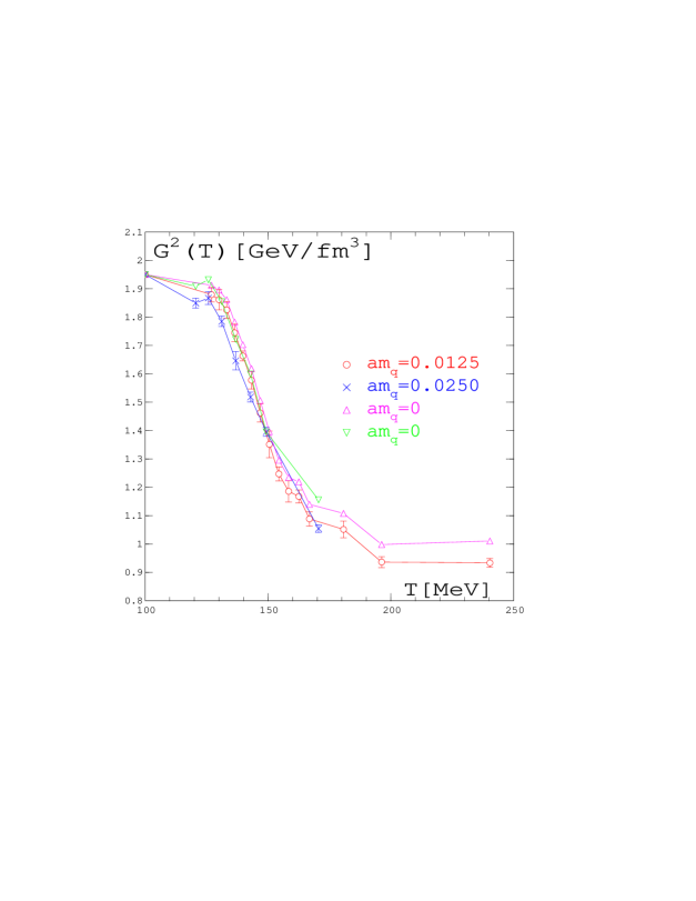
Figure 11: The finite temperature gluon condensate is shown for two light quarks given by the two different lattice masses. We compare these with the corresponding data in the chiral limit shown with the triangles.

chiral order parameter. The values can be seen in the figure 4 of the MILC data [50]. We show these results in the figure 11 for the two different stated masses including the errorbars arising from both the interaction measure and the quark condensate data. We notice that with increasing temperatures that the finite quark mass lowers the gluon condensate. Furthermore, it can be seen in figure 11 that between the temperatures of about $140MeV$ and $160MeV$, which is just below $T_{c}$, both with and without the quark condensates lie very mush together– almost within mutual errorbars. Below and above these values the heavier quark values appear to digress although there are simply too few points to allow for a firm conclusion. This fact clearly shows an additional effect from the restoration of the chiral symmetry on the thermal gluon condensate in the presence of massive quarks. At the highest temperature around $240MeV$ the chiral symmetry for the smaller mass value is about $95\%$ restored. From these results we can understand how the effect of the quark masses together with the restoration of the chiral symmetry changes the size of the gluon condensate. Whereupon we may conclude this discussion of the gluon condensate with two light quark from the MILC97 data [50] by saying that the decondensation of gluons begins considerably below the critical temperature and then slows down for a temperature range above it. Finally we remark that we have taken a compromise value for the vacuum expectation value $G^{2}_{0}=1.95[GeV/fm^{3}]$. This choice for the simulations with dynamical quarks is somewhat larger than the earlier value [36] used for the pure gauge theory in the figure 10. However, it is well within the range of many of the later estimates (for the literature see [15, 16]).
 
IV.4 Gluon and Quark Condensates with more massive Flavors
 
After this evaluation of the gluon condensate for the very light quarks we present the results for two and three moderately light quarks using the Bielefeld data [70, 71, 72]. Thereafter we look at the case with two lighter quarks together with one heavier quark. We shall in general compare the effects of the pure gluon condensate with the maximally estimated effects arising from the quark mass terms, from which we can derive the changes in the thermal properties of the gluon condensate which are due to the dynamical quarks.

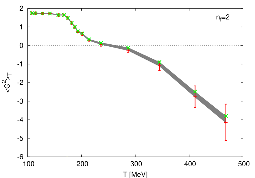
Figure 12: The pure gluon condensate $<G^{2}>_{T}$ in units of $GeV/fm^{3}$ for two moderately light quarks is indicated by the vertical/horizontal lines. The crosses show the estimated maximal effects of the (thermal) quark masses.

We see in Fig. 12 the effects of decondensation of colored quark-gluon fields containing two fairly light dynamical quarks. Here we can clearly notice that above $200~{}MeV$ the difference between the pure gluon condensate with the errorbars and the mass terms appearing with the chiral restoration given by the crosses. The darkened region between the horizontal line and the cross $\times$ is the immediate effect of the thermal mass term caused by the chiral restoration. We can see here that the thermal effects of the mass terms coming from the quark condensate do partially slow down the decondensation of the gluons. This effect we can compare with one of our earlier analyses [64, 65] of the data for $n_{f}=2$ using the even earlier MILC data [48, 49, 50]. For the MILC data the quarks were much lighter– almost an order of magnitude less– from less than $5MeV$ to around $15MeV$. We can now compare the numerical data in the last section for the equation of state shown for different flavor numbers in the figure 9. The gluon condensate we shall denote here as $\langle G^{2}\rangle_{T}$. In the following figures we shall leave out the data for the temperatures above $500MeV$ because of the very large errorbars. Unfortunately, in the following analyses we have lacked the comparable data for the chiral averages for the quark condensate $\langle\bar{\psi}_{q}{\psi}_{q}\rangle_{T}$ which may be associated with the temperature as was the case for the MILC data [50]. Thus the shaded region for the curve above $T_{c}$ gives the estimated maximal range of the effect of the chiral condensate, which in some cases may reach beyond the errorbars.

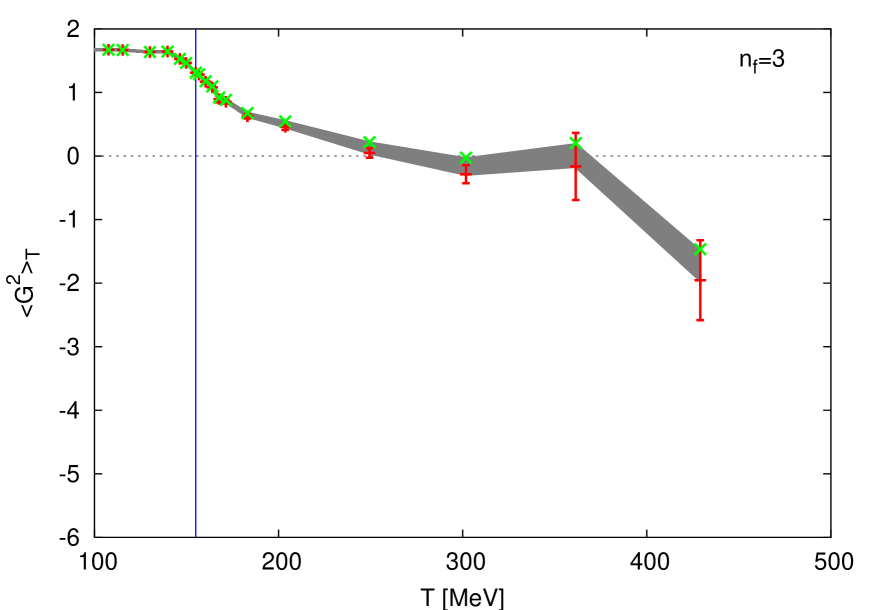
Figure 13: The gluon condensate$<G^{2}>_{T}$ for three middle light quarks in physical units $[GeV/fm^{3}]$.

Next we show in the figure 13 the effects of three moderately light quark flavors on the gluon condensate $\langle G^{2}\rangle_{T}$. A quick examination of this plot shows that the change of $\langle G^{2}\rangle_{T}$ is not so rapid over the same temperature interval as it was the case for the two quark flavors with similar values for the masses. Again we also show here the maximal estimated effect coming out of the masses which when it is taken into account raise the points in the chiral limit. This same effect we have already just seen in the MILC data in figure 11. The small cross $\times$ marks the estimated highest value for $\langle G^{2}\rangle_{T}$ due to the chiral restoration.
 
We show in the next figure 14 the computed results due to the effects of two lighter quark flavors together with one much heavier quark. A quick examination of this drawing shows that the large masses of the dynamical

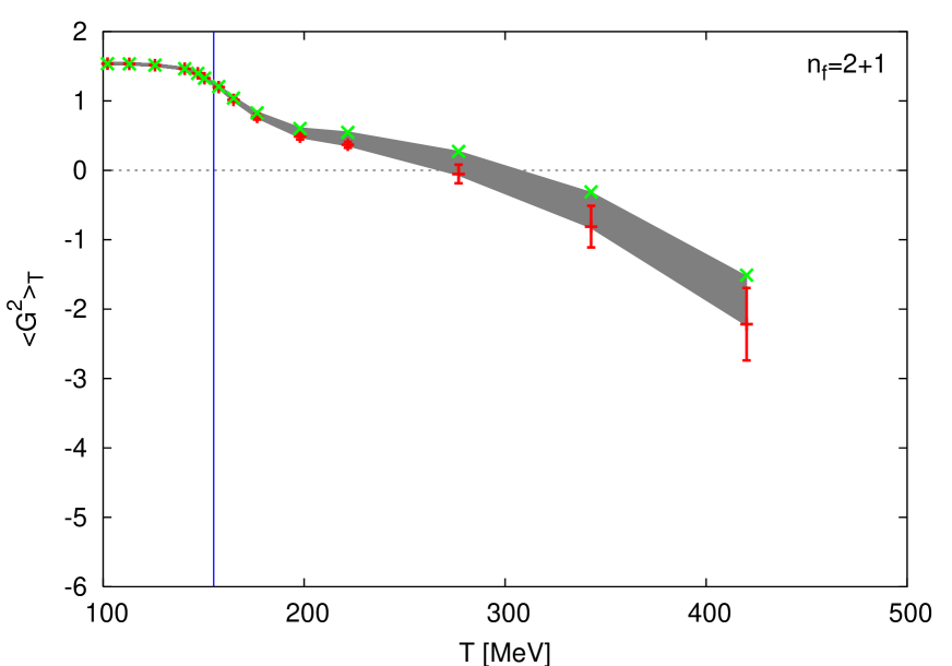
Figure 14: The gluon condensate$<G^{2}>_{T}$ for two moderately light quarks and one much heavier one.

quarks flattens the descent of the decondensation curve even further in comparison to the other two cases. Clearly in this case the mass effects are much larger, which is primarily due to the much more massive ”strange” quark. We see that at higher temperatures the crosses $\times$ are generally above the errorbars for the pure gluon condensate. It is obvious in this case with a heavier quark that we are very far from the situation of the chiral limit. Thus the restoration of the chiral symmetry has much less effect on the gluon condensate in the temperature region above the critical temperature $T_{c}$ and below the deconfinement temperature $T_{d}$ of the pure $SU(3)$ gauge theory. This remark is quite consistent with what we had noted in the last part in the figure 6 where we compared the effects of the quark masses on $<\bar{\psi}\psi>$. We saw there that the larger mass value caused the curves for $<\bar{\psi}\psi>$ to move towards higher values in the coupling $\beta$. Furthermore, the descent of the curves at higher masses is slower, which means that the resoration is less rapid at $T_{c}$ for the more massive dynamical quarks.
 
IV.5 Comparisons of Properties of Gluon Condensates
 
In this segment we discuss some previous work [65] on gluon condensates. In particular, we shall take some special extreme examples out of the cases for which we have numerical and analytical evaluations. In the previous part of this report we have presented some numerical results for the gluon condensates– first for the pure lattice gauge theory, then for the light dynamical quarks with two flavors and finally for the somewhat heavier dynamical quark flavor combination. Therein we had also made some comparitive remarks between the various cases. However, in the preceeding part we have not tried to carefully compare the results for each system. Some years ago such a comparison had been discussed between the gluon condensates arising from the pure $SU(3)$ lattice gauge simulations [10, 37] with those coming from the light dynamical quark data from the MILC collaboration  [50]. As an additional point of comparison [65] a gluon condensate arising from a pure ideal gas of gluons was also introduced with the same ground state value as the QCD vacuum gluon condensate $G^{2}_{0}$, for which the $0.012GeV^{4}$ in often taken [36]. For the ideal gluon condensate the condensation temperature $T_{0}$ was chosen to be $T_{c}$, the deconfinement or critical temperature of the pure lattice gauge theory. We show the results of these comparisons in the figure 15.

Figure 15: The lines show the gluon condensates for SU(3) (solid) and the ideal gluon gas (broken) in comparison with that of the light dynamical quarks denoted by the open circles and the heavier ones with filled squares. The error bars are included when significant. The physical units are for $G^{2}(T)$ $[GeV^{4}]$ and T $[GeV]$.

We now briefly discuss the condensation of an ideal gas of gluons, which we simply write as $G^{2}(T)$ for a finite temperature T. The vacuum expectation value of the pure gluonic system we denote by $G^{2}_{0}$, which has the above known value at zero temperature [36]. From dimensional considerations of the structure of the gluon condensate we can write down the ideal gluon condensate for $T\leq T_{0}$

$$G^{2}(T)~{}=~{}G^{2}_{0}~{}{\left[1~{}-~{}{\left({T\over T_{0}}\right)}^{4}\right]},$$ (38)

where $T_{0}$ is the temperature at which the condensation process ceases. For $T\geq T_{0}$ then $G^{2}(T)~{}=~{}0$. This means that for the gluon condensate of an ideal gas system in equilibrium with its groundstate contribution must vanish above the condensation temperature. This form is just a generalization of the relativistic Bose-Einstein condensation to a four dimensional Euclidean space with $T_{0}$ acting as the critical temperature. Therefore, this equation gives a simple relation between the gluon condensate at a finite temperature $T$ and that at zero temperature. Thus we relate $G^{2}_{0}$ to the QCD vacuum condensate and $T_{0}$ to the deconfinement temperature, which are the corresponding quantities in the previous parts. Although this form for $G^{2}(T)$ as an ideal gluon gas seems at the present time very highly oversimplified, many of the earlier analyses in QCD at finite temperatures with gas models had assumed free gluons. This includes some earlier collaborative work of the author [77] where this type of thermal behavior was assumed as a first approximation to the decondensation of gluons. The extent to which this assumption is valid we are now able to evaluate from the pure $SU(3)$ data [10]. Furthermore, we will make no attempts here at the inclusion of the hadrons in the thermodynamics of the gluon condensate.
 
At the beginning of the previous part we have shown the results [37] for the gluon condensates of the $SU(2)$ and the $SU(3)$ invariant lattice gauge theories over the whole temperature range up to $0.4GeV$. In both cases the uppermost temperature is well above the deconfinement temperature, for which the values of $G^{2}(T)$ are all less than zero as is shown in the figure 10. In the following paragraph we used the argument of Leutwyler [28] in order to explain why the pure gluon condensate remains constant while retaining its vacuum value $G^{2}_{0}$ almost until the temperature reaches $T_{c}$. This effect clearly comes from the strong QCD attractive forces between the gluons. Just below $T_{c}$ the drop in $G^{2}(T)$ signifies the start of the decondensation process. Not only do the gluons coming from the interactions in the vacuum condensate decondense, but the further gluons which are created at these high temperatures also take part in the decondensation process. We now can understand the difference in the behavior for the condensate of the ideal gluon gas which is shown in the figure 15. This gas of free gluons shows a continual decrease even at the low temperatures well under $T_{c}$. At and above $T_{c}$ the ideal gluon gas condensate vanishes so that $G^{2}(T)~{}=~{}0$ for all $T\geq T_{0}$. However, the pure $SU(N_{c})$ gluon condensate continues into negative values of $G^{2}(T)$ as it was shown before in the Figure 10. Thus the difference between the pure lattice gauge thermodynamics and the ideal gluon gas is apparent over the whole range of finite temperatures.
 
The comparison of the gluon condensate from the two light dynamical quarks brings new issues into these considerations. As we have discussed in the preceeding two parts of our work, the presence of the chiral restoration transition changes the thermodynamics completely. In the equation of state $\varepsilon-3p$ for the case of the two light quarks we can see in figure 4 how around $140MeV$ both the curves rise very rapidly. However, at about $200MeV$ the lighter quark mass slows up and even appears to drop a little. Not only is this change at much lower temperatures than the pure gauge results in the figure 1, which show a steady rise beginning at a much higher temperature. The presence of the errorbars in the figure 4 show that the apparent decline of the last point at about $240MeV$ is well within the errorbars of the preceeding point at about $196MeV$. The MILC data is then again plotted for the gluon condensate $G^{2}(T)$ in the figure 11 for which the units are taken as $[GeV/fm^{3}]$ in contrast to the above figure 15. In figure 11 we have connected the points together in order to provide a better view of the changes. The two curves with the errorbars have included the effects of the masses with the quark condensates, which adds some further errors. Nevertheless, we see that the gluon condensate then continues to fall slightly. The unconnected points in the above figure 15 correspond to the unconnected points given in the chiral limit. This fact has been recently pointed out [24, 25] in relation to the ”soft” glue, which disappears much earlier than the hard glue or ”epoxy”. It can also be related to the problem of mass and the presence of mesonic bound states [29] above $T_{c}$, which here denotes the actual critical temperature for the two flavor light quark thermodynamical system. We shall return to this topic in relation to chiral resoration models in a later section of the next part.
 
Finally we are now in a position to discuss the interrelationship between the process of the gluon decondensation and the restoration of chiral symmetry. In the previous three figures 12,  13 and 14 we can see the varying extents that the dynamical quark properties affect the amount the two different broken symmetries are altered with the change of the temperature. As it has been clearly stated by Leutwyler [28], the quantity $<\bar{\psi}\psi>$ acts like an order parameter for the breaking of the chiral symmetry. Actually it is the term $1~{}-~{}<\bar{\psi}\psi>$ in the equation (37) which acts as the restoration quantity for the effects of the quark condensate on the gluon decondensation. In the figure 11 we can see the direct effects of this term which clearly lowers the gluon condensation curve with increasing temperatures due to the restoration of the chiral symmertry. Naturally the bigger effect of the decondensation of the gluons arises in the interaction measure $\Delta_{m}(T)$ in equation (26) from the mass renormalization of the quarks. We see that the antiquark-quark average over the lattice or site average clearly lowers the plaquette average from the links in the interaction measure. This we had already seen in figure 4 for the equation of state for the light dynamical quarks. The equation of state for the dynamical quarks still provides the most important contribution to the decondensation of the gluons. However, the extent to which this last statement is true varies with the number of flavors and the masses of the quarks. Thus we can clearly see the main points of contrast between the decondensation of the gluons in the pure gauge theory and that of the theory with the dynamical quarks.

V.Discussion of Physical Results
 
In this part of our work we shall describe how we are able to calculate some physical quantities from the structure of the equation of state which relate to such phenomena as the possible phase transitions between the hadronic states and the much sought after quark-gluon plasma. First we discuss some models relating to the relativistic high energy collisions at high temperatures and large energy denstiies [15]. Thereafter we shall look at the low energy and low temperature limits where the effective Lagrangians are very useful. We discuss a model for scalar meson dominance with the coupling to the trace of the energy-momentum tensor  [18]. In the last section of this part we look at some other aspects of the equation of state which arise at temperatures well below the critical temperature. In our last comments at the end we mention how these considerations may relate to some newer lattice simulations not included in the presented data.
 
 
V.1 Phenomenological Models of Quark and Gluon Properties
 
One of the most successful models for the highly relativistic nucleus-nucleus collisions was proposed almost a quarter of a century ago by Bjorken [91]. He suggested a senario where a quark-gluon plasma should survive on a time scale of $5fm/c$, where c is the speed of light which we have usually taken to be unity. During this short time the collision region maintains a longitudinal flow which should be described according to the laws of relativistic hydrodynamics [92].
 
The dynamical structure of the Bjorken model can be reduced to that of a 1+1 dimensional Lorentz boost invariant system in the time and space coordinates t and z. Bjorken, however, then chose to represent the flow in terms of the ”light cone” variables, for which he took the propertime $\tau=\sqrt{t^{2}-z^{2}}$ and the rapidity $y={1\over 2}\ln{{t+z}\over{t-z}}$. These variables are useful in maintaining the boost invariance. In addition to the usual energy momentum conservation Bjorken further postulated [4, 15] a conservation of the entropy density $s=\beta(\varepsilon+p)$, where $\beta$ is the inverse temperature. Out of these assumptions one gets for the fourvector entropy density $s^{\mu}=su^{\mu}$ the conservation law

$${\partial}_{\mu}s^{\mu}=0,$$ (39)

where $u^{\mu}$ is the fluid fourvelocity with $u_{\mu}u^{\mu}=1$. After setting the initial propertime $\tau_{0}$ with the entropy density $s(\tau_{0})$, one finds simply the solution [91]

$${s(\tau)\over{s(\tau_{0})}}={{\tau_{0}}\over{\tau}}.$$ (40)

In terms of the variables $\tau$ and $y$ the entropy density stays on the lightcone. This result may be interpreted as the entropy content per unit rapidity is a constant of the motion [91]. Furthermore, this result may be related to the Bjorken equation of state, which may be written as

$$\varepsilon=p(3+\Delta_{1}).$$ (41)

Comparably the entropy density for the Bjorken model may be written as

$$s={\beta}p(4+\Delta_{1}).$$ (42)

The new quantity $\Delta_{1}$ is defined in the Bjorken model as follows:

$$\Delta_{1}={T\over{n}}\left(dn\over{dT}\right).$$ (43)

In the rest of this very original work Bjorken [91] showed how these equations can be used for the effective number of plasma degrees of freedom $n(T)$ which he had originally proposed to have a sharp rise for the temperatures above the transition temperature around $200MeV$. An important application of an extension of the Bjorken equation of state (42) has been found in the calculation of the radiative energy loss of high energy partons traversing an expanding QCD plasma [93].
 
For us in this work what is really significant here is that the Bjorken equation of state leads to corrections beyond the ideal gas as well as the simple bag model pictures. Bjorken [91] also pointed out that the general features of the hydrodynamical expansion follow from the positivity condition on the trace of the energy momentum tensor. In fact, this statement would imply that the positive definiteness condition on the trace of the energy momentum tensor is such that the trace itself would only be zero in the absence of all interactions.
 
More recently the hydrodynamical models [15] have been brought in relation to the Bjorken model. In this context the well known ideas of relativistic hydrodynamics [92] have been extended for use in the explanation of the data from heavy ion collisions undergoing a hydrodynamical expansion [94]. At the present time there is a considerable amount of phenomonological work in this direction.
 
V.2 Theoretical Models for the Quark and Gluon Properties
 
In this section we shall look into some of the theoretically important statistical models for strong interaction physics. Some of these relate to the recent RHIC data [15]. First we mention the Statistical Bootstrap Model (SBM) which was earlier regarded for providing the limiting temperature for hadronic physics [87]. In the following paragraphs we shall discuss here some further models involving the quarks and gluons in large statistical systems.
 
Now we discuss the properties of resonances at high temperatures and densities which are typical of high energy particle collisions. The particle creation process at such high energies is the starting point for the SBM first introduced in the midsixties by Rolf Hagedorn [87]. Earlier pure statistical models based on ideal gas theory with the proper statistics related the temperature directly to the center of mass energy. These models had in common an exponential energy distribution relating to the probabilities of each of the hadronic states. However, Hagedorn had noted that in high energy proton-proton collisions that the masses $m$ are distributed in what appeared to be asymptotically an exponentially rising mass spectrum $\rho(m)$. This spectrum included the entire known resonance structure of hadronic particle physics. Furthermore, he then postulated that the mass spectrum approached asymptotically the energy level density $\sigma(E)$ in the high energy limit. After having calculated $\sigma(E)$ from the partitiion function with $\rho(m)$ for a gas of particles and resonances, he invoked the statistical bootstrap condition relating $\rho(m)$ asymptotically to $\sigma(E)$. However, this condition only held true up to a particular temperature $T_{0}=158\pm 3[MeV]$, when certain statistical assumptions were made on the pararmeters of $\rho(m)$. Nevertheless, this temperature $T_{0}$ had found its special place in the particle phenomenology of that time through its place as the limiting temperature. A more contemporary understanding of this resonance formation is found from an examination of this Hagedorn temperature and the partition thermodynamics [88]. The hadronic phase with all the included resonances can only exist below $T_{0}$. This statistical theory was clearly modeled on the particle states which were known at that time. The sense of such a model with a limiting temperature has changed drastically with the inclusion of quarks as the basic constituents of the hadrons. More recently some further implications in relation to the quark-gluon transition have been discussed [14]. The SBM serves as a starting point of a statistical treatment of the hadrons with their constituent quarks and interacting gluons.
 
In the early nineteen seventies not long after the initial development [16, 20, 56, 57] of QCD as the gauge theory for the strong interactions between the quarks, there was a great deal interest in finding analytical solutions for particular cases. The discovery of the instanton solution [79] in 1975 of the $SU(2)$ Yang-Mills field and its further development [15, 17] were important starting point for an approximate analytical approach to nonperturbative QCD. After a brief initial excitement giving hope of a discovered particle in the years directly following these discoveries, there began an era of long and systemmatic investigation of these rather intriguing mathematical objects [80, 81] in the name of the instanton gases and liquids with various forms [15]. More recently the importance of the bound states and the instanton molecules [83] has become clearer. Furthermore, it was noted that the fermionic (quark) zero modes can be related to the axial anomaly [21]. This leads to the properties of the chiral symmetry breaking and its restoration [25] as we had mentioned previously. A more lengthy discussion of these ideas can be found [15, 16] which give details on the explicit structure. The relation to some earlier lattice computations is also quite important (see [5] in section 17.6). Furthermore, the thermodyanmical properties of the instantons relating to the topological charge $Q^{2}_{T}$ can be evaluated on the lattice using the thermal susceptibility in equation (31) as indicated above in the equation (32). There are also related lattice simulations on the flux tubes (see [5] section 17.7) for further discussions on the newer evaluations. Further work involving the instanton has been presented by Ilgenfritz and Shuryak [82] in a simple model at finite temperature. The role of the instantons has been generally discussed by Shuryak [15] in relation to the transition from hadrons to the quark gluon plasma. As we mentioned in the last part, there was an attempt [77] to formulate a mean field model of an instanton (caloron) gas at finite temperature in contact with the condensate of an ideal gluon gas.
 
The early finite temperature simulations [2, 5] for lattice gauge theory provided information of the thermodynamical functions around the critical temperature $T_{c}$. The discussion of some previous results for the gluon and quark condensates were derived from some of the earlier simulations. In this relationship we must mention that the values of the vacuum condensates were calculated out of sum rules [36, 96]. The early use of the finite temperature lattice results [22, 27] has had a significant part in thedevelopment in such computations. These authors had evaluated the gluon condensate in the separate parts arising from the chromoelectric and chromomagnetic fields with the thermally averaged condensates as seen in reference [27] in their Figure 4. Unfortunately in the earlier lattice data the temperature scale was very hard to determine. In 1994 this changed significantly through a better evaluation of the lattice beta function [9] for the SU(2) gauge theory. Even in these earlier times the use of these ideas was apparent in the study of the hadron to quark-gluon transition [14].
 
Finally we mention some other work involving QCD at finite temperature and density. First we remark on the models involving quasiparticles [89, 90] which take into consideration the lattice properties of the high temperature states. These models generally reproduce the lattice data above about $2T_{c}$. Some recent lattice work [69] using a QCD model with two flavors of adjoint quarks provides a very unique picture of both the deconfinement and chiral phase transitions. It shows both a chiral second order transition and a first order deconfinement phase transition. However, it can be seen in their Figure 12 showing the chiral condensate in terms of the coupling $\beta$ and the lattice quark mass ${m_{q}}a$ that in this model the deconfinement transition appears at a lower temperature than that of the chiral restoration. In fact they estimate [69] that $T_{c}/T_{d}\approx 7.8(2)$, which means that the critical temperature remains very far above the deconfinement temperature.
 
In this section we have related the results of numerical simulations which are usually represented as ratios of the quantities to powers of the temperature to the actual physical quantities like the pressure, energy density, entropy density. We can arrive at a form of the equation of state which can be used to find other physical quantities. We look again at the first pure gauge theory simulations at finite temperature, which provided for us a way to arrive at the thermodynamical quantities in the gluon condensate.
 
V.3 Scaling Properties in Matter
 
There are a number prominent examples where the parameters in the effective actions for physical processes need be determined by some further rules. Important among these is the Brown-Rho Scaling properties for finite densities $\rho$, which we have mentioned in the introduction [23, 24]. It is commonly given by a scaling function ${\Phi}(\rho)$ for the different hadrons (for a general description see reference [24]) in the following form:

$${\Phi}(\rho)~{}\approx~{}{{f^{*}_{\pi}(\rho)}\over{{f_{\pi}}}}~{}\approx~{}{{m^{*}_{\sigma}(\rho)}\over{{m_{\sigma}}}}~{}\approx~{}{{m^{*}_{V}(\rho)}\over{{f_{V}}}}~{}\approx~{}{{M^{*}(\rho)}\over{{M}}}.$$ (44)

The expressions $f^{*}_{\pi}(\rho)$ and $f_{\pi}$ are the pion decay constants in the medium with the density $\rho$ and that of the vacuum respectively. In this same notation (with the $*$ above) the masses of the scalar $\sigma$ and vector $V$ particles are compared with the corresponding values in their different media. In the last ratio there appears the nucleon mass $M$. Nevertheless, it is important in all cases to stress that the Brown-Rho Scaling is a mean field relation which emerges at the tree level from the effective Lagrangian for the chiral fields [23, 24]. This scaling rule may be further approximately generalized to the quark condensates are related to the hadron masses.

$${{m^{*}}\over{m}}~{}\approx~{}{{\langle{\bar{q}q}\rangle^{*}}\over{\langle{\bar{q}q}\rangle}}.$$ (45)

This case is referred to as the ”Nambu scaling” which usually includes the temperature dependence [27, 24]. This property is a generic feature of the linear sigma model. It is then supposed to be upheld as the temperature rises towards the chiral restoration temperature. It was noted in a recent work how the matter induced modifications of certain resonances fitting the masses of various particles [78] causes a shift as well as a change of shape of various particles and resonances. Further work on the nature of the chiral restoration [25], used an earlier work [65] of the author to discuss how the mixed phase [29] appeared after the chiral restoration has started, but before the deconfinement temperature in the pure gauge theory. We have already seen in the last part that the Figure 15 can be interpreted in terms of the soft glue, which disappears rather quickly with the chiral restoration, while the hard glue (epoxy) remains well above $T_{c}$. There these properties were associated with the slowing up of the decondensation processes of the light dynamical quarks. The heavier quarks gave a much flatter decondensation curve for which the two different properties are harder to recognize. Furthermore, it is expected that the correlations above $T_{c}$ are, indeed, very significant and have an important relationship to the recent RHIC experements [24, 25].
 
V.4 Scalar meson dominance
 
In this section we look into the model of Freund and Nambu [18] for the dominance of the scalar meson. This property is deeply rooted in the empirical observations of the meson and baryon mass splittings. Already in 1968 they had proposed that the classical meson field $\varphi(x)$ be coupled to the trace of the energy momentum tensor $\theta^{\mu}_{\mu}$. A more detailed discussion of the relation of these (pseudo)scalar fields to the energy momentum tensor one finds in section three of Bogoliubov and Shirkov [84]. In this model the nonhomogeneous Klein-Gordon equation could be written in the form

$$(\Box~{}-~{}m^{2})\varphi(x)~{}=~{}g{\theta^{\mu}_{\mu}},$$ (46)

whereby $m$ is the scalar meson mass and $g$ its coupling to the trace. Here it is important for us to note that this coupling $g$ differs from the usual QCD coupling in its place in the model, which was, of course, not known at that time. In the following paragraphs we briefly sketch the basic arguments for this model which we shall later relate phenomenologially to the process of gluon decondensation.
 
From the usual properties of field theory one can derive the trace of the energy momentum tensor [84]${\theta^{\mu}_{\mu}}$ from the Lagrangian $\mathcal{L}(\varphi,{\partial}_{\mu}{\varphi})$. Out of the above form of the Klein-Gordon equation (46) for the scalar field $\varphi(x)$ Freund and Nambu derived [18] their effective Lagrangian by taking into account the appropriate boundry conditions. It took the following form:

$$\mathcal{L}(g,\varphi)~{}=~{}{\frac{1}{2}}{\partial}_{\mu}{\varphi}R(x)^{-1}{\partial}_{\mu}{\varphi}~{}-~{}{\frac{1}{2}}m^{2}{\varphi}^{2},$$ (47)

where $R(x)$ is defined to be $(1+2g\varphi(x))$. After a careful consideration of the form of the Lagrangian they [18] introduced a new field $\psi(x)$, which is defined by

$$\psi(x)~{}=~{}g^{-1}R(x)^{1/2}.$$ (48)

This field transformation yielded a new Lagrangian $\mathcal{L}^{\prime}(g,\psi)$ in terms of the new field in the form

$$\mathcal{L}^{\prime}(g,\psi)~{}=~{}{\frac{1}{2}}({\partial}_{\mu}{\psi})^{2}~{}+~{}{\frac{1}{4}}m^{2}{\psi}^{2}~{}-~{}{\frac{1}{8}}m^{2}g^{2}{\psi}^{4}-~{}{\frac{m^{2}}{8g^{2}}}.$$ (49)

Furthermore, it must be noted here that the sign is wrong for the usual ”mass term” in the Lagrangian density. This situation provides the conditions [85] of a degenerate vacuum which gives rise to Goldstone bosons upon quantization. It can be easily seen after one further change to $\psi_{\pm}$ as $\psi{\pm}1/g$. Then we find this change of the fields results in

$$\mathcal{L}^{\prime}(g,{\psi}_{\pm})~{}=~{}{\frac{1}{2}}({\partial}_{\mu}{\psi}_{\pm})^{2}~{}-~{}{\frac{1}{2}}m^{2}{\psi}_{\pm}^{2}~{}\pm~{}{\frac{1}{2}}m^{2}g{\psi}_{\pm}^{3}-~{}{\frac{1}{8}}m^{2}g^{2}{\psi}_{\pm}^{4},$$ (50)

which is equal [18] to the original Lagrangian $\mathcal{L}(g,\varphi)$. As we would expect, the dynamical properties of both of these fields $\psi_{\pm}$ correspond to the same mass $m$. Either one of the Lagrangians $\mathcal{L}(g,\psi)$ or $\mathcal{L}^{\prime}(g,{\psi}_{\pm})$ yields after quantization the same physical properties in the corresponding S Matrix as the original one $\mathcal{L}(g,\varphi)$ derived [18] in equation (47). Thereby it is clear that there is a twofold degeneracy in the vacuum of the quantized theory. This model even in its unquantized form was recognized by Bruno Zumino to break the scale invariance [85] as well as allow for the Goldstone bosons. Furthermore, this situation leads to the fact that the coupling of the trace $g{\theta^{\mu}_{\mu}}$ in the nonhomogeneous term of the Klein-Gordon equation (46) relates directly to the square of the mass times the strength of the transformed scalar field. Thus the Lagrangian of Freund and Nambu provides a simple model for the scalar field dominance of the trace of the energy momentum tensor $\theta^{\mu}_{\mu}$.
 
The quantized theory can be achieved from the classical one in the usual way from the Poisson brackets [84]. The momentum $\pi(x)$ canonically conjugate to $\varphi(x))$ from the original Lagrangian $\mathcal{L}(g,\varphi)$ is gotten as the Poisson bracket ${\frac{1}{2}}\{R(x)^{-1},{\partial}_{0}{\varphi}\}$. Because of this form of the Poisson brackets the ordinary equal-time commutation relations do not specify the canonical commutator but only the mixed commutator in the form

$${\frac{1}{2}}\{R(x^{\prime})^{-1},[\varphi(x),{\partial^{\prime}}_{0}{\varphi(x^{\prime})}]\}_{x_{0}=x_{0}^{\prime}}~{}=~{}i\delta^{3}(x-x^{\prime}).$$ (51)

From this form and the specification that $[\varphi(x),\varphi(x^{\prime})]_{x_{0}=x_{0}^{\prime}}$ and $[{\partial}_{0}{\varphi(x)},{\partial}_{0}^{\prime}{\varphi(x^{\prime})}]_{x_{0}=x_{0}^{\prime}}$ both identically vanish allows the calculation of the equal time field momenta $[\pi(x),\pi(x^{\prime})]_{x_{0}=x_{0}^{\prime}}$. With the definition that at the same point

$$[R(x)^{-1},R(x)^{-1}]\delta^{3}(0)~{}=~{}0.$$ (52)

it is possible to evaluate the Schwinger commutator [34, 35] for $\theta_{00}(x)$. More important to us in the present work is the fact that Freund and Nambu have evaluated the corresponding commutator for the trace of the energy momentum tensor $\theta^{\mu}_{\mu}(x)$ as

$$[\theta^{\mu}_{\mu}(x),\theta^{\mu}_{\mu}(x^{\prime})]_{x_{0}=x_{0}^{\prime}}~{}=~{}-4i[\theta_{0i}(x)~{}+~{}\theta_{0i}(x^{\prime})]{\partial}_{i}\delta^{3}(x-x^{\prime}).$$ (53)

This feature allows that the trace of the energy momentum tensor be treated as a quantum field. These authors [18] have suggested that this commutation relationship be considered as a general feature of the theory of hadrons. Thus the Lagrangian $\mathcal{L}(g,\varphi)$ in their formulation provides a rather simple model for scalar field dominance from the trace of the energy momentum tensor. These results can be understood from the transformation properties of the action integral under the scale transformations [85].
 
Next we work out the special case of the scalar meson field $\varphi(x)$ with the mass $m$ for the ground state structure in the simple bag model. For simplicity we assume a simple cubic region with the sides of length $1[fm]$ for the discrete momentum representation [84]. The solution for the zero mode of the nonhomogeneous Klein-Gordon equation (46) for the scalar field $\varphi_{0}(x)$ using the isotropic bag model value [14] of the energy momentum tensor ${\theta}^{\mu}_{\mu 0}~{}=~{}4{\mathcal{B}}$. In this case we find a simple time dependent solution $\varphi(x_{0})$ with the zero spatial modes for the scalar meson ground state solution

$$\varphi_{0}(x_{0})~{}=~{}{4g{\mathcal{B}}\over{m^{2}}}\left(cos(mx_{0})-1\right),$$ (54)

where we have taken $\varphi_{0}(0)=0$ and ${\dot{\varphi}_{0}}(0)=0$. This special case is so easily solvable since there is no spatial dependence coming into the field equation from the trace of the energy momentum tensor. Thereupon the value of the amplitude only involves the nonhomogeneous term divided by the mass squared. Then this special case yields just the simple harmonic oscillator type of solution. Now we see for the chiral limit for the solution in equation (54) that the solution goes to the finite value

$$\lim m\rightarrow 0,~{}~{}~{}\varphi_{0}(x_{0})~{}\rightarrow~{}{2g{\mathcal{B}}}{x_{0}}^{2}.$$ (55)

Thereby the small mass limit for the zero momentum state has a finite value which is positive definite from ${x_{0}}^{2}$. Since this zero momentum state solution has no spatial dependence in it, we may replace $x_{0}$ by the propertime $\tau$ at $\vec{x}=0$. Then we find at the center for $\lim m\rightarrow 0$ that

$$\varphi_{0}(\tau)~{}=~{}{2g{\mathcal{B}}}{\tau}^{2}.$$ (56)

Thus we would expect the scalar field for the hadron to grow quadratically in the proper time, for which only on the light cone does it totally disappear. Furthermore, after a little further investigation, we find that all the higher mode solutions in the discrete momentum representation would involve free spatial wave solutions set to zero at the boundries of the box. However, these solutions involve an infinite sum in each spatial dimension.
 
As a concluding point to this discussion we comment on the interesting possibilities of this model from the view of the equation of state. Next we shall consider the trace of the total energy momentum tensor $T^{\mu}_{\mu}(T)$ as a function of the temperature. In the simple solution found above for $T=0$ we saw that the trace appeared only in the solution form the bag constant $4{\mathcal{B}}$. Then we would expect that even at finite temperatures this same type of dependence on the equation of state would directly enter into the solution. For the sake of simplicity we shall now only consider the effects of the decondensation for the pure $SU(3)$ gluons as shown in the Figure 10. We recall that the decondensation of gluons starts around the deconfinement temperature of about $270MeV$, where the equation of state undergoes a rapid growth as shown in the first figure for the temperature dependence. If we assume for simplicity that the scalar meson state in the simplest case is only changed by the added temperature dependence of the trace, then we would expect a rapid growth in the scalar field $\varphi_{0}(x_{0})$ as a function of the temperature. Thus our boundstate solution for the nonhomogenous Klein-Gordon Equation (46) given in (54), shows rapid changes in the classical scalar meson field just above the decondensation temperature. Furthermore, if we take the lowest scalar meson, the $\sigma$, with a mean mass $m_{\sigma}=600MeV$ and a full width at least $400MeV$, this added energy from the decondensing gluons could perhaps be enough to bring about a single decay of a virtual scalar meson state into two pions. In no sense are we advocating that this very rough picture should provide a realistic explanation for the effects of gluon condensation in QCD. However, it is generally consistent with the decay of the scalar meson in its very simplest case.
 
 
V.5 Entropy for the Hadronic Ground State
 
In this section we look at a different situation involving the equation of state for the quarks making up the ground state structure of the hadrons. We start this investigation with the introduction of the entropy density $s(T)$ for a thermal quark system at very low temperatures $T$. Here we assume the singlet structure for the confined quarks in the hadronic bag which should hold for temperatures well below the critical temperature $T_{c}$. Herewith we are able to include some aspects of the groundstate structure in the equation of state.
 
We start with the energy density $\varepsilon(T)$ and pressure $p(T)$ of a confined colored quark gas for $T\ll T_{c}$. We use the First Law of Thermodynamics to include the classical heat density contribution

$$s(T)T~{}=~{}\varepsilon(T)~{}+~{}p(T)~{}-~{}\mu_{q}{n_{q}(T)},$$ (57)

where $\mu_{q}$ is the quark chemical potential and $n_{q}(T)$ is quark density distribution function for a single quark flavor. We may rearrange this equation using the fact that the thermal average of the trace of the energy momentum tensor providess the equation of state as given in the equation (2), which now takes the form

$$\theta^{\mu}_{\mu}(T)~{}=~{}s(T)T~{}-~{}4p(T)~{}+~{}\mu_{q}{n_{q}(T)}.$$ (58)

For the bag model in the limiting case that the temperature approaches to zero we use $p=-\mathcal{B}$, where, as before, $\mathcal{B}$ is the bag constant [16] independent of the temperature. Clearly in this limit $~{}s(T)T~{}$ vanishes. Furthermore, in the above equation of state we replace $n_{q}(T)$ with the Fermi distribution function $f(\mu_{q},T)$ times $n_{0}$, which is the quark number density in the bag at zero temperature.

$${\theta^{\mu}_{\mu}}_{0}~{}=~{}4\mathcal{B}~{}+~{}\mu_{q}{n_{0}}f(\mu_{q}),$$ (59)

In the low temperature limit $f(\mu_{q},T)$ is simply a step function so that $f(\mu_{q})$ becomes the normalized particle distribution at zero temperature. As we have previously explained in the introduction, the trace of the energy momentum tensor can be related to the gluon and quark vacuum expectation values arising from the operator product expansion  [16, 36, 28] following from equation (6) for ${\theta^{\mu}_{\mu}}_{0}$. Thus we have, as before, included the important vacuum contributions of both operator dimensions three and four to the equation of state, which are both clearly independent of the temperature.  
 
In relation to the previous section on scalar meson dominance we choose as a simple special case that of the meson with the same light quarks surrounded by nuclear matter as an example for this investigation. Then we have from the Fermi statistics using the quark-antiquark symmetry $~{}\mu_{\bar{q}}~{}=~{}-\mu_{q}~{}$ and for the antiquark quantum density distribution function $~{}n_{\bar{q}}(T)~{}=~{}n_{0}(1~{}-~{}f(\mu_{q},T))~{}$. Thus in the limit of zero temperature we have simply the expected value for the bag model [14, 52]

$${\theta^{\mu}_{\mu}}_{0}~{}=~{}4\mathcal{B}.$$ (60)

For the moment we take as a first approximation the case that we consider the value  [16] of only the gluon condensate as about $~{}1.95[GeV/fm^{3}]~{}$. Here we use the fact that the values of the quark condensate for the light quarks are almost negligible. Thus we note that for this special case the bag constant $~{}\mathcal{B}~{}$ is rather big– just under $0.5GeV$. However, if we take T finite and small, the gluon condensate does not change very much [28, 37] until we reach rather high temperatures.
 
Nevertheless, the constituent entropy at very low temperatures due to the color degrees of freedom does have a very important contribution to the equation of state. In the singlet state it has been shown from the structure of the hadronic density matrix [97] that the quantum ground state entropy for the colored constituent quarks and antiquarks contribute an internal entropy with the value $\ln{3}$. Although the hadrons themselves are pure states with zero quantum entropy, the constituents do have a finite entropy. In fact, in the singlet groundstate the quarks(antiquarks) have the maximum entropy of pure (color) mixing. Then the equation of state for the bag containing the constituents can be written with the additional contribution from the mixing of the colors in the quarks and antiquarks treated as separate consitiuents. The total constituent entropy density is then $~{}2s_{M}~{}$ for both the quarks and the antiquarks treated as separate entities.
 
Now we consider the total equation of state $T^{\mu}_{\mu}(T)$ containing both the groundstate and the thermal states using the decomposition in Equation (1) together with the above Equations (58) and (59) for the meson made up of the constituent quarks and antiquarks. The equation of state for the color singlet quarks in the mesonic bag is given by

$$T^{\mu}_{\mu}(T)~{}=~{}(2s_{M}~{}+~{}s(T))T~{}-~{}4(p(T)~{}-~{}\mathcal{B})~{}+~{}\mu_{q}n_{0}(2f(\mu_{q},T)~{}-~{}1).$$ (61)

At very low temperatures we would expect that $~{}s(T)~{}$ and $~{}p(T)~{}$ both to remain insignificant so that the main change in the equation of state is the value of $2s_{M}~{}=~{}1.824[1/fm^{3}]$. Physically we could relate this effect either to a lowered bag constant or a raised chemical potential. Thereby we may be able to see how much the finite temperature changes the actual value of the entropy due to the color mixing with its corresponding effect upon the equation of state.
 
Along this same line we have also investigated a baryonic model at finite $T$ including the ground state entropy for colored quarks. Here we have studied the relation of the temperature and chemical potential to $\mathcal{B}$. In this previous work we calculated explicitly the effects of colored quark entropy on the bag pressure [98] in terms of the temperature. The general equation of state is rather similar to Equation (61) with the exception that the groundstate contains the quark entropy with the factor of $3s_{B}$. Following this work we looked into the effects of the quark chemical potential [99] on the entropy for a color superconductor.

VI. Conclusions, Deductions and Evaluations
 
In this last part of our discussions of lattice calculations for the equation of state we bring together some of the main points in this report. An important aspect investigated in the Introduction was the breaking of both the scale and conformal symmetries when the strong nuclear interactions are present. This situation was very well stated by Stefan Pokorski in his book on Gauge Field Theories: ”Scale invariance cannot be an exact symmetry of the real world. If it were, all the particles would have to be massless or their mass spectra continuous.” This statement in itself is not so very surprising when we are only considering massive particles like quarks or hadrons. However, because of the trace or conformal anomaly we saw in the second part from the simulation of pure gauge fields that this type of symmetry breaking continues for strongly interacting gluons even at very high temperatures. In the third part when the massive quarks are present in the simulations, the breaking of scale and conformal symmetries have a somewhat different relation to the phase transition because of the process of the restoration of the broken chiral symmetry which changes the properties of the quarks in the transition from the confined phase to the deconfined one. It is known, in fact, that the Wilson or Polyakov loop as the order parameter of the pure gauge deconfinement transition ceased to provide this property in the presence of dynamical quarks [2, 3, 5]. In this context we looked explicitly at the chiral anomaly in relation to the breaking of chiral symmetry in the presence of dynamical quarks. The thermodynamics is best related through the susceptibilies to the chiral condensate, which becomes itself an order parameter in the limit of vanishing quark masses. These results led the way to the explicit numerical evaluations of the thermodynamical properties of the gluon and quark condensates in the following sections of the next part. Finally we presented models which more directly relate to physical results from experiments. Now we summarize and expand upon some of the work which we have presented.
 
VI.1 Summary of Results and Related Ideas
 
Throughout this work we have mentioned the importance of the ranges of the temperatures computed by using lattice gauge theory with the $SU(N)$ color symmetry both without and with different numbers and masses of quarks present. By using the lattice data from numerous simulations we have plotted the various physical quantities in terms of the temperature. Without entering into the computational details we have investigated the numerical results in relation to the theoretical content of the simulation. We were in the above mentioned cases able to determine the thermodynamical functions like the pressure, energy density, entropy density and the resulting equation of state for the quarks and gluons as a function of the temperature. These results allowed us to see the growth of these thermodynamical quantities above the transition temperature, from which we could examine the quark and gluon condensates as well as compute the thermal properties in the determined related phases.
 
There were a number of other important lattice studies of various different quark and gluon properties whose data and resuts we have not directly used. The starting point was in 1974 the ”Confinement of quarks” by Kenneth Wilson [1, 100] where he not only set out the formalism of the lattice gauge theory by quantizing in Euclidean space-time, but also proposed the method of evaluation using the Feynman path integrals with the strong-coupling approximation. This very original work also introduced the Wilson action including the quarks. An alternative approach [102] to the lattice fermions was proposed by John Kogut and Leonard Susskind known as the ”staggered fermions.” Most of the data presented above uses this formulation for the dynamical fermions on the lattice since it is somewhat better for the type of computations which have been carried out. The numerous works of Michael Creutz were very essential to these numerical simulations [2, 103]. In the earlier times around 1980 there were many very active groups which contributed greatly to the development of the lattice gauge computations with some very important results [104, 105, 106, 107] for pure $SU(N)$ lattice gauge simulations. These works provided the starting point for many of the later computations of the MILC and Bielefeld groups– for further literature see [11, 12, 103].
 
In recent years there have been considerable progress in the simulations with finite chemical potentials on the lattice. The above discussions have not included these many extensive computations [109, 110] with dynamical quarks who included the chemical potentials. Only in the above very special example of the single flavored meson at low temperatures have we directly included the effects the quark-antiquark chemical potential. This particular case has its sole importance for the analysis of the model of a meson for the equation of state at very low temperatures. Others with dynamical quarks who included the chemical potentials were some works on the phase diagram by Fodor and Katz [109] as well as the more recent work done in collaboration of Bielefeld and Swansea [110]. These results we have not included with our analysis. There are also further important contributions from the CP-PACS Collaboration with two heavier quark flavors using the Wilson action for which we were unable to set the temperature scale to find thermodynamical functions out of the computed ratios [108]. Although all these works are very interesting, the form of the data as well as the values are often not in the temperature range where a comparison with the quantities are easily carried out.
 
VI.2 Implications from the Analysis
 
There has oftentimes been a problem with the interpretation of some of the results from the numerous lattice computations due to the many general statements arising out of the ideal gas models. In numerous papers and even in some very highly respected text books there have appeared statements where the expected approximate equality of $\varepsilon$ and $3P$ becomes very nearly realized within a few integral mutiples of the critical temperature. However, we have seen above that within the range of the present numerical data from lattice gauge simulations all of statements of this type are clearly not fulfilled. In the earlier parts of this report we have seen the results for the equations of state in the figures 1, 2, 4, and 9. All of these evaluations clearly show directly that these equations of state in terms of the temperature remain finite well above the critical or deconfinement temperature. As we have already explicitly pointed out in the text, with the possible exception of our figure 4, all the other plots show clearly a monotonical growth of the equation of state as a function of the temperature. Perhaps one possible source of misunderstanding of the lattice data lies in the representation as ratios with the $T^{N}$ powers divided out. From the computational side this representation is very useful for direct comparisons with the high temperature limits for lattices of different sizes. However, for the interaction measure, which is defined as a ratio there are thermal contributions to the energy density which are different from those arising in the pressure. The difference $\varepsilon-3p$ has contributions of lower powers and logarithmic terms in the temperature which appear to go to zero in the high temperature limit when divided by the higher power. Thus the interpretation coming from the appearance of the numerical results from the lattice presented as ratios can be quite misleading for the curves with a finite or vanishing limiting behavior. Here, as we have stated above, it is important that such terms be written in terms of the well understood thermodynamical quantites, which must diverge in the infinite temperature limit in accordance with the leading powers. Furthermore, as one perhaps could expect from the formulation of the laws of thermodynamics, we are also able to described the equation of state using exact differential forms which relate directly the known anomalies to the actual physical quantities [52, 64]. In this general manner the action as a formal expression of quantum field theory is also clearly related to the general structure of the equation of state (see Appendix B).
 
It was recently discussed how the lattice results show that even at temperatures much larger than the deconfinement temperature the thermodynamically related observables like the pressure ratio, the energy density ratio, the interaction measure and the baryon number density ratio at different chemical potentials still deviate by more than $20\%$ from their respective relativistic ideal gas values [111]. These authors consider two special model cases: the two phase model and the mixed phase model, which they have quite appropriately named. The direct comparisons with the lattice data for the 2+1 flavor cases [70, 71] and [109] provided insight into both the critical behavior and the asymptotic approach at high temperatures. In the case of the interaction measure the two phase model had a much sharper peak at the critical temperature than provided by the lattice data. However, the mixed phase model the peak provided much smaller peaks in the interaction measure. For the other ratios involving the pressure, energy density and the baryon number density the results of the comparisons with the lattice data were generally quite similar.
 
VI.3 Applications to Physical Processes
 
We have already mentioned in the previous part of this report the properties of the equation of state at low temperatures for the study of the hadronic structure. In this temperature region the thermodynamical functions included in the equation of state are much harder to compute using the numerical simulations of finite temperature QCD on the lattice. Nevertheless, there has recently been considerable progress on the numerical computations of correlations between quarks and antiquarks at these lower temperatures in certain model cases [112]. Certainly a part of this computational difficulty lies in complicated quantum structure in the low temperature thermodynamics providing for the basic properties of the hadronic ground state. In this context we have previously looked into the role of the quantum entropy [97] in the discussion of the stability of the various quantum states– particularly relating to the singlet hadronic states.
 
The thermodynamics of quarks and gluons in the confined region is of great interest in the examination of the formation of particle states below the deconfinement temperature. The recent computations of the quark-antiquark free energies [112] using the renormalized Polyakov loop has provided considerable new insight into the short distance interactions between the quarks and the antiquarks over a large range of temperatures. The results from these numerical simulations evaluate the color averaged and the color singlet free energies for static quark-antiquark sources placed in a thermal gluonic heat bath. An important procedure [112] in these calculations is the renormalization of these free energies using the short distance properties of the zero temperature heavy quark potential. This procedure leads to the definition of the renormalized Polyakov loop as an order parameter for the deconfinement phase transition of the $SU(3)$ gauge invariant field theory. The color averaged free energy $F_{\bar{q}q}(r,T)$ of a static quark-antiquark pair acting as sources in a thermal medium is related up to a function of the temperature to the thermally averaged product of the color averaged Polyakov loops at two different spatial points separated by a distance $r$. The color singlet free energy $F_{1}(r,T)$ is related to both the thermal and color averaged product of the gauge field variables. The significance of these results lies in the fact that at very short distances these two differently defined free energies become the same up to a factor of $T\ln 9$. Thus in the limit of short distances it was found [112] that

$$\lim_{r\to 0}[F_{\bar{q}q}(r,T)~{}-~{}F_{1}(r,T)]~{}=~{}T\ln 9,~{}~{}~{}\forall{T}.$$ (62)

However, at larger values of the distance $r$ there are additional contributions to the colored averaged free energy coming from the octet states, which vanish at small distances. More recently the actual effective running coupling at finite temperatures has been calculated for both the quenched [115] and two flavor [116] QCD from the derivative of the free energy with respect to the separation $r$ between the quarks and antiquarks. In a later work these latter authors [117] look at the singlet internal energy and entropy at large separations and higher temperatures about $1.3T_{c}$. However, in the case of small separations these authors note that both $U_{1}(r,T)$ and $TS_{1}(r,T)$ suffer from lattice artifacts which result in the same problems for the singlet free energy.
 
Next we mention some ideas closely related to these results but arise from quite different considerations for low temperature quantum critical systems. First we recall from thermodynamics that the free energy $F$ and the internal energy $U$ are related through the entropy $S$ by a simple transformation: $F=U-TS$, whereby we can write that $S=-{\frac{\partial{F}}{\partial{T}}}$. Thus we see that for finite temperatures we have a simple relation to the entropy. However, as mentioned in the last part, the entropy of the hadronic groundstate has the role of the mixing of the colors. It has been recently pointed out [113] that for one-dimensional quantum critical systems the entropy near criticality can be clearly divided into two separate parts– the bulk part arising from the partition function and the boundry terms relating to the groundstate degeneracy $d_{g}$. This approach had been successfully applied in the past [114] to such important problems as the Kondo effect and the Heisenberg ferromagnet. Here we are interested in some different applications in relation to quark string models for the discussed computations on the lattice of Polyakov loop correlations [112]. We recall in our above discussion of the quantum ground state of the hadronic singlet state that the associated entropy of the quark and antiquark is $\ln 3$. If we regard the quark and antiquark as the end of a one-dimensional string, then we may associate the boundary entropy $\ln{d_{g}}$ as arising from the groundstate degeneracy $d_{g}~{}=~{}3$ for the static quark and antiquark. Thus by the addition of entropies we may write the total boundry entropy for the two static sources as $2\ln 3$. All other sources of entropy we may associate with the bulk entropy in the string [113], which we assume here is mainly due to the gluons. Finally if we assume that the internal energy at zero temperature is just the static quark-antiquark potential, we are thereby able to identify the term $~{}T\ln 9$ as arising from the groundstate entropy.
 
We now recall some of the general results of our report as written above. The light quarks first go through the chiral restoration transition at a temperature $T_{c}$ then the effects of deconfinement actually will appear at a higher temperature $T_{d}$. The nature including even the order of these transitions appears to depend greatly upon the number of flavors as well as the masses. The heavier quarks show the separation between the transitions much less clearly. However, in all cases both the scaling and the conformal symmetries are still broken at much higher temperatures well above both of these transitions. We see from the physical equation of state that the very high temperatures provide a further symmetry breaking which is not present in the QCD vacuum contributions. The properties of the Brown-Rho scaling are important to the actual particle structure when surrounded by hot dense matter. Also recently the mass and the width of the sigma resonance have been calculated [118] by locating the pole in the pion-pion scattering amplitude with the quantum numbers of the vacuum. The quarks and gluons are strongly correlated even well above the transition temperatures. There is also an effect of the running coupling [115, 116] involving the confining part of the quark-antiquark interaction well above $T_{c}$. In a very recent article Gerry Brown and collaborators posed a critical question on the results of the recent heavy ion experiments at Brookhaven National Laboratory. Therein they indicate the nature of the high temperature state by the statement [120]: ”We suggest that the new form of matter found just above $T_{c}$ by the Relativistic Heavy Ion Collider is made up of tightly bound quark-antiquark pairs,…” Their observation gives further motivation for the present investigations of the correlations and interactions at temperatures above $T_{c}$.
 
Finally in the two appendices we add some detail to the discussions of the models and the physical currents. There we formally discuss the actual physical meaning of these currents as expansion parameters and forces arising from the breaking of the scale and conformal symmetry. We take the well known example described in Appendix A – the MIT Bag model. The bag constant itself arises in the trace to make it nonzero. In the Appendix B we discuss how the dilatation and conformal currents are related to both the equation of state and the gluon condensates. We show these relations are best understood from the integral or the dual forms of these currents.

Acknowledgements The author wants to thank all the colleagues in Bielefeld, especially Rolf Baier, Jürgen Engels, Frithjof Karsch, and Helmut Satz for their help on many parts of this work. He would also like to recognize important discussions with Dietrich Bödecker, Rajiv Gavai, Sourendu Gupta, Olaf Karczmarek, Peter Kolb, Edwin Laermann, Mikko Laine, Andreas Peikert, Bengt Petersson, Peter Petreczky, Paul Romatschke, York Schröder, Edward Shuryak, Ismail Zahed and Felix Zantow. Further he is very grateful to Carleton DeTar for providing the MILC97 data. He thankfully recognizes the efforts of Graham Boyd for his earlier work in an essential collaboration on this subject. The author wants to acknowledge Abdel-Nasser Tawfik for his help with the preparation of some useful figures and some earlier collaborative discussions. To Ivan Andrić, Neven Bilić, Ivan Dadić, Jerzy Lukierski and Krzysztof Redlich he wishes to express his thanks for their help and friendship as hosts in Zagreb and Wroclaw in the Fulbright Scholar Program a well as many scientific discussions. He is very indebted to Gerry Brown both as a teacher and presently as the editor for his interest, ideas and many suggestions on this subject. Finally he is grateful to the Pennsylvania State University for the Research Award from the University Commonwealth College.
 
 
APPENDIX A: Phenomenological Models for Confinement
 
In this added section we sketch the properties of some of the most prominent phenomenological models used in the theory of strong interactions to explain the observation of quark comfinement. It is meant as an extension to the introduction for the added properties.
 
1. The MIT bag model was proposed as a model for the extended hadrons which contain free quarks inside a small volume. The action [13] with the internal energy density ${\mathcal{B}}$ is written in the following form:

$$\mathcal{W}~{}=~{}{\int}^{t_{2}}_{t_{1}}dt{{\int}_{R}}{d^{3}}r[{\frac{1}{2}}\dot{\phi}^{2}~{}-~{}{\frac{1}{2}}(\vec{\nabla}\phi)^{2}~{}-~{}{\mathcal{B}}],$$ (63)

where ${\phi}(t,r)$ is the prototype of a hadronic field, which are the partonic or hadronic constituents, and $R$ and $(t_{1},t_{2})$ are the space and time regions for the ”bag”. This action provides the field equations inside the bag

$$-{\Box}\phi(x)~{}=~{}0$$ (64)

and on the surface

$${\hat{n}}\cdot{\frac{\partial{\vec{R}}}{\partial t}}\dot{\phi}~{}+~{}{\hat{n}}\cdot{\vec{\nabla}\phi}=~{}0.$$ (65)

Then the bag condition at the surface becomes

$${\frac{1}{2}}\dot{\phi}^{2}~{}-~{}{\frac{1}{2}}(\vec{\nabla}\phi)^{2}~{}=~{}{\mathcal{B}}.$$ (66)

These three equations are basic to the MIT bag model. We note that the structure of this model is not directly in correspondence with QCD because of the time of development of the fields.
 
2. There have been many further developments on the equation of state for many cases involving bag models in a more general form. One can propose a form for the energy $E(T,V)$ containing the bag term as ${E_{0}}(V)={\mathcal{B}}V$. As a correction one often adds the thermal radiation terms of the Stefan- Boltzmann type ${{\sigma}_{SB}T^{4}}V$. However, this form may be extended to a more general energy equation of the following type:

$$~{}E(T,V)~{}=~{}{E_{0}}(V)~{}+~{}E^{\prime}(T,V).$$ (67)

The pressure is defined by the usual relation $p=-({\partial}E/{\partial}V)_{T}$. When the free energy density $f^{\prime}(T)$ of the finite temperature part is scaled with a temperature $\vartheta$ so that $f^{\prime}(T)=T{\phi}({\vartheta}/T)$, where $\phi$ is only a function of ${\vartheta}/T$, then the equation of state is just

$$~{}p~{}=~{}-{\mathcal{B}}~{}+~{}\gamma{\varepsilon}^{\prime}.$$ (68)

The constant is defined $\gamma=-d(\ln{\vartheta})/d(\ln{V})$ for the energy density at finite temperature ${\varepsilon}^{\prime}$. For the ultrarelativistic gas $\gamma=1/3$, which yields the known relationship to the bag constant  [13, 14]. The form of this equation for the relativistic gas is similar to the Debye equation of state for solids at low temperatures. In the Debye theory of solids $\gamma$ is often referred to as the ”Grüneisen constant.” This approach of separating the groundstate and thermal states allows us to write a very general form of the equation of state.
 
3. The chiral bag model [21] has additional properties in relation to QCD. This new structure is often referred to as ”The Cheshire Cat Mechanism.” For simplicity one usually looks at a model in 1+1 dimensions. The action $S$ is then decomposed into three parts

$$~{}S~{}=~{}S_{V}~{}+~{}S_{\tilde{V}}~{}+~{}S_{\partial{V}}$$ (69)

where for the fermions

$$~{}S_{V}~{}=~{}\int_{V}d^{2}x{\bar{\psi}}i{\gamma}^{\mu}{\partial}_{\mu}{\psi}~{}+...,$$ (70)

while for the bosons

$$~{}S_{\tilde{V}}~{}=~{}\int_{\tilde{V}}d^{2}x{\frac{1}{2}}({\partial}_{\mu}{\phi})^{2}~{}+....$$ (71)

The additional surface term becomes with the value of $f~{}=~{}{\frac{1}{\sqrt{4\pi}}}$ and $d{\Sigma}^{\mu}$ is the surface area with the normal vector ${n}_{\mu}$ so that

$$~{}S_{\partial{V}}~{}=~{}\int_{\partial{V}}d{\Sigma}^{\mu}\{{\frac{1}{2}}{n}_{\mu}{\bar{\psi}}\exp{(i{\gamma}_{5}{\phi}/f)}{\psi}\}~{}+....$$ (72)

APPENDIX B: Mathematical Forms and Physical Currents
 
In this appendix we provide some additional information on some particular differential forms relating to the various discussed broken symmetries due to the properties of the strong interacions. There are two different types forms relating to the structures of the anomalies, which are related to the axial and conformal anomalies respectively. In the former case there are already a large number of works [34, 20] relating to the chiral symmetry breaking and the axial anomaly, for which there is a very well known differential four-form $\mathcal{A}d{\Omega}$. Furthermore, there is the related Chern-Simons Form $d{\mathcal{B}}$, which can be represented as a three-form on a three dimensional closed surface. One can also discuss the physical interpretation of this form which is related to the topological charge. These ideas together with the properties of the chiral symmetry breaking in relation to the instanton solutions is discussed in the book of Edward Shuryak [15].
 
The scale and conformal symmetry breaking can be similarly related to the conformal or trace anomaly. In the above work we have found the presence of a finite trace of the energy-momentum tensor relating to the equation of state and the QCD sum rules. It is known in quantum field theory that classically the trace of the energy-momentum tensor is zero. In the following we derive (introduce) the corresponding three-forms under the names dyxle for the scale breaking and the fourspan for the special conformal symmetry breaking. The actual physical meanings for these currents and charges have been previously discussed [35]. The actual interpretion of these as energy flux and shearing forces has been given not so long ago by the author [64], upon which we shall now briefly expand.
 
The dilatation current $D^{\mu}$ has already been defined above in terms of the position four-vector $x^{\mu}$ and the energy momentum tensor $T^{\mu\nu}$ as simply the product $x_{\alpha}T^{\mu\alpha}$ as moments of the energy density. In the case of the general energy-momentum conservation [33, 35] one can find quite simply a relation to the equation of state [52, 64]. We now look into a volume in four dimensional space-time ${\Omega}$ containing all the quarks and gluons at a fixed temperature $T$ in equilibrium. The flow equation holds when the energy momentum and all the (color) currents are strictly conserved over the closed bounding surface $\partial{\Omega}$ of the properly oriented four-volume ${\Omega}$, which yields

$$\oint_{\partial{\Omega}}{\cal D}_{\mu}dS^{\mu}~{}=~{}\int_{{\Omega}}T^{\mu}_{\mu}d{\Omega},$$ (73)

We have already introduced [64] the dyxle three-form as  ${\cal D}_{\mu}dS^{\mu}$ on the closed three dimensional surface $\partial{\Omega}$, which is simply just the divergence in the four dimensional Minkowski space. The dyxle is the dual to the dilatation current written as the one-form $D_{\mu}dx^{\mu}$ in the usual four dimensional space-time. In this context the dilatation current $D_{\mu}dx^{\mu}$ acts as if it were a streaching force over the space-time infinitesimal $dx^{\mu}$. Whereas its dual form in space-time represents the divergence of this three dimensional closed surface acting as the boundry for the four dimensional volume ${\Omega}$. On the right hand side of (73) the integrated four-form  $\int_{{\Omega}}T^{\mu}_{\mu}d{\Omega}$ is an action or energy moment integral involving the equation of state. Since we assume here the positivity of the trace so that $T^{\mu}_{\mu}>0$, we can conclude that this action integral is a positive quantity. It acts as the color averaged source of the energy flux. This action integral gets quantized with the fields through the renormalization process.
 
The analogous three-forms can be defined for the four special conformal currents which we shall collectively call the fourspan. The analogous dual forms are derived from the equation in a similar manner to that previously done for the dyxle [52, 64]. The results for the four conformal currents yield the four three-forms ${\cal K}^{\alpha}_{\mu}dS^{\mu}$ is derived similarly from the following equation:

$$\oint_{\partial{\Omega}}{\cal K}^{\alpha}_{\mu}dS^{\mu}~{}=~{}\int_{{\Omega}}{2{x^{\alpha}}}T^{\mu}_{\mu}d{\Omega},$$ (74)

We point out here that for the fourspan the source terms are the first moments in space-time of the equation of state. Furthermore, the physical nature of the quantities ${\cal K}^{\alpha}_{\mu}$ as the special conformal currents can be seen to be related to the shearing forces which destroy the conformal symmetry in all the four directions. The effect of the fourspan is analogous to the dyxle along the radial line in the four dimensions. In summary these five three-forms provide the mathematical structure for the known breaking of the scale and conformal symmetries for the strong (nuclear) interaction.
 
As an example of the formal statements above we work out the analytical properties of these forms may be exactly calculated in the special case of the well known [13] MIT bag model. The scaling properties associated with the trace of its energy-momentum tensor we have noted above. This relationship yields in the above equation (2) simply $\theta^{\mu}_{\mu}=4{\cal B}$. This result gives an exact solution for the dilatation current $D^{\mu}(x)$ of the form:

$$D^{\mu}(x)~{}=~{}{\cal B}x^{\mu}.$$ (75)

It is clear that this solution is a special case of the above general form $x_{\nu}T^{\mu\nu}$ for the bag model. Similarly we derive the special forms for the four conformal currents $K^{\alpha\mu}(x)$ using the same general structure as for the dilatation current. Here there are two different types of solutions: (a) $\alpha=\mu$ and (b) $\alpha\neq\mu$. In the first case (a) using the propertime $\tau^{2}=x_{\mu}x^{\mu}$ with the implicit summation over the indices $\mu$, we have for a single value of the index chosen from $\alpha=\mu=0$ for the temporal case

$$K^{00}(x)~{}=~{}{\cal B}(2(x^{0})^{2}-\tau^{2}),$$ (76)

while for $\iota=1,2,3$, where $\iota=\alpha=\mu\neq 0$ the spatial case yields

$$K^{\iota\iota}(x)~{}=~{}{\cal B}(2(x^{\iota})^{2}+\tau^{2}).$$ (77)

For the case (b) we have $\iota\neq\kappa$ so that the result for $\iota,\kappa=0,1,2,3$ is just

$$K^{\iota\kappa}(x)~{}=~{}2{\cal B}x^{\iota}x^{\kappa}.$$ (78)

Thus we see that in case (a) in the equations (76) and we (77) have various combinations of quadratic terms depending upon which value of $\iota=0$ or $\iota=1,2,3$. $K^{00}(x)$ is just a four dimensional shearing force. Furthermore, we notice that it is truly positive definite so that for both spacelike and timelike events in the bag it remains always positive. However, in case (b) in equation (78) we find simply bilinear terms in two different space-time coordinates. The simplicity of these solutions for $D^{\mu}(x)$ and $K^{\alpha\mu}(x)$ arises form the fact that the energy momentum tensor and the metric tensor are both diagonal in the Minkowski metric for the bag model. All the conformal currents $K^{\alpha\mu}(x)$ act like internal shearing forces which all go against the preservation of the angular symmetries which includes the breaking of the scale symmetry associated with $D^{\mu}(x)$.

References

-
[1]
K. G. Wilson,
Physical Review, D14 (1974) 2455.
-
[2]
M. Creutz,
Quarks, Gluons and Lattices,
Cambridge University Press, Cambridge 1983.
-
[3]
I. Montvay and G. Münster,
Quantum Field Theory on the
Lattice, Cambridge University Press, Cambridge 1996.
-
[4]
M. Le Bellac,
Thermal Field Theory ,
Cambridge University Press, Cambridge 1996.
-
[5]
H. J. Rothe,Lattice Gauge Theories,
An Introduction, World Scientific, Singapore, 1992, Third Edition, 2005.
- [6] J. Engels, F. Karsch, H. Satz and I. Montvay, Nuclear Physics (1982) 545.
- [7] J. Engels, J. Fingberg, K. Redlich, H. Satz and M. Weber, Zeitschrift für Physik , 341 (1989).
- [8] J. Engels, J. Fingberg, F. Karsch, D. Miller and M. Weber, Physics Letters , 625 (1990).
- [9] J. Engels, F. Karsch and K. Redlich, Nuclear Physics, , 295 (1995).
- [10] G. Boyd, J. Engels, F. Karsch, E. Laermann, C. Legeland, M. Lütgemeier and B. Petersson, Physical Review Letters , 4169 (1995); Nuclear Physics (1996) 419.
- [11] H. Satz, , North-Holland, Amsterdam, 1981.
- [12] J. Cleymans, R.V.Gavai and E. Suhonen, Physics Reports 130 (1986) 217.
- [13] A. Chodos, R. Jaffe, K. Johnson, C. B. Thorn and V. F. Weisskopf, Physical Review D, 9 (1974) 3471.
- [14] G. E. Brown, A.D. Jackson, H.A. Bethe and P.M.Pizzochero, Nuclear Physics A560 (1993) 1035.
- [15] E. V. Shuryak, , World Scientific, Singapore (Second Edition) 2004.
- [16] J. F. Donoghue, E. Golowich and B. R. Holstein, , Cambridge University Press, Cambridge, England, 1992.
- [17] G. ’tHooft, , World Scientific, Singapore,2005.
- [18] P. G. O. Freund and Y. Nambu, Physical Review, (1968) 1741.
- [19] Y. Nambu and J. Jona-Lasinio, Physical Review, (1961) 345.
- [20] T. Kugo, , Springer Verlag, Berlin, 1997.
- [21] M. A. Nowak, M. Rho and I. Zahed, , World Scientific, Singapore, 1996.
- [22] C. Adami, T. Hatsuda and I. Zahed, Physical Review D, , (1991) 921.
- [23] G. E. Brown and M. Rho, Physical Review Letters (1991) 2720.
- [24] G. E. Brown and M. Rho, Physics Reports 363 (2002) 85.
- [25] G. E. Brown, L. Grandchamp, C.-H. Lee and M. Rho, Physics Reports 391 (2004) 353.
- [26] I. Zahed and G. E. Brown, Physics Reports 142 (1986) 1.
- [27] V. Koch and G. E. Brown, Nuclear Physics (1993) 345.
- [28] H. Leutwyler, “Deconfinement and Chiral Symmetry” in , Vol. 2, P. M. Zerwas and H. A. Kastrup (Eds.), World Scientific, Singapore, 1993, pp. 693-716.
- [29] H.-J. Park, C.-H. Lee and G. E. Brown, ”The Problem of Mass: Mesonic Bound States Above .” e-print Archive: hep-ph/0503016.
- [30] S. L. Adler, Physical Review (1969) 2426.
- [31] S. L. Adler and W. A. Bardeen, Physical Review (1969) 1517.
- [32] J. S. Bell and R. Jackiw, Nuovo Cimento (1969) 47.
- [33] S. B. Treiman, R. Jackiw, B Zumino and E. Witten (Eds.), , R. Jackiw, ”Field Theoretical Investigations in Current Algebra”, pp. 81-210; World Scientific, Singapore, 1985,
- [34] R. A. Bertlmann, , Oxford Science Publications, Oxford, 1996.
- [35] S. B. Treiman, R. Jackiw, B Zumino and E. Witten (Eds.) , R. Jackiw, ”Topological Investigations of Quantized Gauge Theories”, pp. 211-359; World Scientific, Singapore, 1985.
- [36] M. A. Shifman, A. I Vainshtein and V. I. Zakharov, Nuclear Physics (1979) 385,448,519.
- [37] G. Boyd and D. E. Miller, “The Temperature Dependence of the Gluon Condensate from Lattice Gauge Theory”, Bielefeld Preprint, BI-TP 96/28, August 1996, E-print Archive:hep-ph/9608482.
- [38] J. Engels, J. Fingberg, D. E. Miller and M. Weber, Nuclear Physics (1992) 501.
- [39] J. Engels, F. Karsch and T Scheideler, Nuclear Physics (2000) 303.
- [40] E. Laermann, Proceedings of the International Workshop on Lattice QCD on Parallel Computers, Nuclear Physics B (Proceedings Supplement), , 180 (1998).
- [41] F. C. Hansen and H. Leutwyler, Nuclear Physics , 201 (1991).
- [42] R. J. Crewther, Physical Review Letters, (1972) 1421.
- [43] M. S. Chanowitz and J. Ellis, Physics Letters, , 397 (1972); Physical Review, , 2490 (1973).
- [44] S. L. Adler, J. C. Collins and A. Duncan, Physical Review , 1712 (1977).
- [45] P. Gerber and H. Leutwyler, Nuclear Physics (1989) 387.
- [46] J. C. Collins, A. Duncan and S. D. Joglekar, Physical Review , 438 (1977).
- [47] N. K. Nielsen, Nuclear Physics (1977) 212.
- [48] T. Blum, L. Kärkkäinen, D. Toussaint and S. Gottlieb (MILC Collaboration), Physical Review (1995) 5153.
- [49] C. Bernard, T. Blum, C. E. DeTar, S. Gottlieb, U. M. Heller, J. E. Hetrick, L. Kärkkäinen, C. McNiele, K. Rummukainen, R. L. Sugar, D. Toussaint, and M. Wingate (MILC Collaboration), Proceedings of Lattice’96, Nuclear Physics B(Proceedings Supplement) (1997) 442.
- [50] C. Bernard, T. Blum, C. DeTar, S. Gottlieb, K. Rummukainen, U. M. Heller, J. E. Hetrick, D. Toussaint, L. Kärkkäinen, R. L. Sugar and M. Wingate (MILC Collaboration), Physical Review (1997) 6861.
- [51] J.Engels, R. Joswig, F. Karsch, E. Laermann, M. Lütgemeier, and B. Petersson, Physics Letters , 210 (1997).
- [52] D. E. Miller, Acta Physica Polonica, (1997) 2937.
- [53] D. Zwanziger, Physical Review Letters (2005) 182301.
- [54] V. N. Gribov, Nuclear Physics, (1978) 1.
- [55] A. D. Linde, Physics Letters, (1980) 289.
- [56] T. Muta, , World Scientific, Singapore, (Second Edition) 1998.
- [57] St. Pokorski, , Cambridge University Press, Cambridge, England, Second Edition, 2000.
- [58] Y. Deng, Proceedings of Lattice’88, Nuclear Physics B (Proceedings Supplement) (1989) 334.
- [59] F. R. Brown, N. H. Christ, Y. Deng, M. Gao and T. J. Woch, Physical Review Letters (1988) 2038.
- [60] R. V. Gavai, S. Gupta and S. Mukherjee, Physical Review (2005) 074013.
- [61] K. Kajantie, M. Laine, K. Rummukainen and Y. Schröder, Physical Review (2003) 105008.
- [62] M. Laine and Y. Schröder, Physical Review (2006) 085009.
- [63] E. Laermann, Proceedings of the XVth International Symposium on Lattice Field Theory, Nuclear Physics B (Proceedings Supplement), , 114 (1998).
- [64] D. E. Miller, ”Anomalous Currents and Gluon Condensates in QCD at Finite Temperature”, Preprint Vienna ESI 733 (1999); Bielefeld BI-TP99/20 (1999), E-print Archive: hep-ph/9907535.
- [65] D. E. Miller, ”Gluon condensates at finite Temperature”, Bielefeld Preprint BI-TP-2000/17, e-print Archive: hep-ph/0008031.
- [66] E. Bessel-Hagen, Mathematische Annalen, , 258 (1921).
- [67] J. C. Collins and M. J. Perry, Physical Review Letters (1975) 1353.
- [68] S. Holtmann, ”Goldstone mode effects and critical behavior of QCD with two light quark flavors”, Doctoral Dissertation, Universität Bielefeld, June 2004.
- [69] J. Engels, S. Holtmann and T. Schulze, Nuclear Physics (2005) 357.
- [70] F. Karsch, E. Laermann, and A. Peikert, Physics Letters (2000) 447.
- [71] F. Karsch, E. Laermann, and A. Peikert, Nuclear Physics (2001) 579.
- [72] A. Peikert, ”QCD thermodynamics with 2 + 1 quark flavours in lattice simulations”, Doctoral Dissertation, Univeristät Bielefeld (2000) unpublished.
- [73] C. Bernard, T. Burch, C. DeTar, J. Osborn, St. Gottlieb, E. B. Gregory, D. Toussaint, U. M. Heller and R. Sugar, Physical Review (2005) 034504.
- [74] C. Bernard, T. Burch, C. DeTar, St. Gottlieb, U. M. Heller, J. E. Hetrick, L. Levkova, F. Maresca, D. B. Renner, R. Sugar and D. Toussaint, ”The Equation of State with 2+1 Flavors of Quarks,” hep-lat/0509053, Sept. 2005.
- [75] C. McNeile, ”An Estimate of the Chiral Condensate from unquenched Lattice QCD”, arXiv:hep-lat/0504006. 8.April 2005.
- [76] C. Bernard et al. (MILC Collaboration), Physical Review (2001)054506; 117501.
- [77] N. Bilić and D. E. Miller, Nuclear Physics (1981) 347.
- [78] E. Shuryak and G. E. Brown, Nuclear Physics (2003) 322.
- [79] A. A. Belalvin, A. M. Polyakov, A. A. Schwartz and Yu. S. Tyupkin, Physics Letters (1975) 85.
- [80] R. Rajaraman, , North-Holland, Amsterdam 1982.
- [81] A. D. Schwarz, , Springer-Verlag, Berlin, 1993.
- [82] E. M. Ilgenfritz and E. V. Shuryak, Physics Letters (1994) 263.
- [83] G. E. Brown, C-H. Lee, M. Rho and E. Shuryak, ”The bound states and Instanton molecules”, arXiv:hep-ph/0312175.
- [84] N. N. Bogoliubov and D. V. Shirkov, , Wiley-Interscience, New York, Third Edition, 1980.
- [85] S. Deser, M. Grisaru, and Hugh Pendleton, Ed. , B. Zumino, ”Effective Lagrangians and Broken Symmetries”, pp.437-500, MIT Press, Cambridge, MA, 1970.
- [86] E. Laermann, Proceedings of Quarkmatter’96, Nuclear Physics , 1c (1996); F. Karsch et al., Proceedings of Lattice’96, Nuclear Physics B(Proceedings Supplement), , 413 (1997).
- [87] R. Hagedorn, Supplemento al Nuovo Cimento, Volume III, 147 (1965).
- [88] Ph. Blanchard, S. Fortunato and H. Satz, European Physical Journal (2004) 361.
- [89] A. Peshier, B Kämpfer and G. Soff, ”From QCD lattice calculations to the equation of state of quark matter”, arXiv:hep-ph/0206229.
- [90] A. Rebhan and P. Romatschke, ”HTL quasiparticle models for deconfined QCD at finite chemical potential”, arXiv:hep-ph/0304294.
- [91] J. D. Bjorken, Physical Review (1983) 140.
- [92] L. D. Landau and E. M. Lifshitz, , Volume VI, ”Hydrodynamics”, Pergammon Press, Oxford, 1980.
- [93] R. Baier, Yu. L. Dokshitzer, A. H. Mueller and D. Schiff, Physical Review (1998) 1706.
- [94] D. H. Rischke, ”Fluid Dynamics for Relativistic Nuclear Collisions” in , J. Cleymans, H. B. Geyer and F. G. Scholtz (Eds.) Springer-Verlag, Berlin, 1999, pp. 21-70.
- [95] S. Eidelman et al., Physics Letters (2004): Particle Data Group.
- [96] St. Narison, , Cambridge University Press, Cambridge, England, 2004.
- [97] D. E. Miller, European Physical Journal (2004) 435;arXiv:hep-ph/0306302.
- [98] D. E. Miller and A.-N. Tawfik, Journal of Physics, (2004) 731; arXiv:hep-ph/0309139.
- [99] D. E. Miller and A.-N. Tawfik, Acta Physica Polonica, (2004) 2165; arXiv:hep-ph/0405175.
- [100] K. G. Wilson, in , A. Zichichi, Editor, Plenum, New York, 1977.
- [101] J. Smit,, Cambridge University Press, Cambridge, England, 2004.
- [102] J. Kogut and L. Susskind, Physical Review (1975) 395.
- [103] C. Rebbi, , World Scientific, Singapore, 1983.
- [104] J. Kuti, J. Polonyi and K. Szachanyi, Physics Letters (1981) 199.
- [105] L. D. McLerran and B. Svetitsky, Physics Letters (1981) 195.
- [106] J. Engels, F. Karsch, I. Montvay, and H. Satz, Physics Letters (1981) 89.
- [107] J. Kogut, M. Stone, H. W. Wyld, W. R. Gibbs, J. Shigemitsu, S. H. Shenker and D. K. Sinclair, Physical Review Letters, (1983) 393.
- [108] A. Ali Khan et al. (CP-PACS Collaboration) Physical Review (2002) 074510.
- [109] Z. Fodor and S. Katz, Physics Letters (2002) 87.
- [110] C.R. Allton, M. Döring, S. Ejiri, S.J. Hands, O. Kaczmarek, F. Karsch, E. Laermann and K. Redlich, (Bielefeld Swansea Collaboration), Physical Review (2005) 054508.
- [111] A. S. Khvorostukin, V. V. Skovov, V. D. Toneev and K. Redlich, ”Lattice QCD Constraints on the Nuclear Equation of State”, ArXiv:nucl-th/0605069.
- [112] O. Kaczmarek, F. Karsch, P. Pretreczky and F. Zantow, Physics Letters (2002) 41.
- [113] D. Friedan and A. Konechny, Physical Review Letters (2004) 030402.
- [114] I. Affleck and A. W. W. Ludwig, Physical Review Letters (1991) 161.
- [115] O. Kaczmarek, F. Karsch, F. Zantow and P. Pretreczky, Physical Review (2004) 074505.
- [116] O. Kaczmarek and F. Zantow, Physical Review (2005) 114510.
- [117] O. Kaczmarek and F. Zantow, ”Static quark-antiquark interactions at zero and finite temperature QCD. II. Quark-antiquark internal energy and entropy,” arXiv:hep-lat/0506019.
- [118] L. Caprini, G. Colangelo and H. Leutwyler, Physical Review Letters (2006) 132001.
- [119] M. R. Pennington, Physical Review Letters (2006) 011601.
- [120] G. E. Brown, B. A. Gelman and M. Rho, Physical Review Letters (2006) 132301.
- [121] J. D. Walecka, , Oxford, Oxford, 1995
- [122] H. Flanders, , Second Edition, Dover, New York, 1989.