THE ROLE OF POLARIZED VALONS IN THE FLAVOR SYMMETRY BREAKING OF NUCLEON SEA

Abstract

Next-to-leading order approximation of the quark helicity distributions are used in the frame work of polarized valon model. The flavor-asymmetry in the light-quark sea of the nucleon can be obtained from the contributions of unbroken sea quark distributions. We employ the polarized valon model and extract the flavor-broken light sea distributions which are modeled with the help of a Pauli-blocking ansatz. Using this ansatz, we can obtain broken polarized valon distributions. From there and by employing convolution integral, broken sea quark distributions are obtainable in this frame work. 0ur results for $\delta u$, $\delta d$, $\delta\bar{u}$, $\delta\bar{d}$ and $\delta\bar{s}$ are in good agreement with recent experimental data for polarized parton distribution from HERMES experimental group and also with GRSV model. Some information on orbital angular momentum as a main ingredient of total nucleon spin are given. The $Q^{2}$ evolution of this quantity, using the polarized valon model is investigated.

Received (Day Month Year)Revised (Day Month Year)

PACS Nos.: 13.60.Hb, 12.39.-x, 13.88.+e.

1 Introduction

In contrast to most deep inelastic structure functions which are correspond to spin average scattering, it will be possible to extend the discussion to the situation where, for instance, the lepton beam and nucleon target are polarized in the longitudinal direction. The polarized parton distributions of the nucleon have been intensively studied in recent years [1]^-[17]. The conclusion has been that the experimental data dictate a negatively polarized anti-quark component, and show a tendency toward a positive polarization of gluons.

Presently there are a lot of precise data [18]^-[27] on the polarized structure functions of the nucleon. Recently HERMES experimental group has reported some data [28] for the quark helicity distributions in the nucleon for up, down, and strange quarks from semi-inclusive deep-inelastic scattering. Among experimental groups, HERMES as a second generation experiment can be used to study the spin structure of the nucleon by measuring not only inclusive but also semi-inclusive and exclusive processes in deep-inelastic lepton scattering. Semi-inclusive deep-inelastic is a powerful tool to determine the separate contributions of polarized distribution of $\delta q{(x)}$ of the quarks and anti quarks of flavor $f$ to the total spin of the nucleon. From analytical point of view, all polarized parton distributions including the polarized light symmetric sea distribution can be obtained in this letter through the polarized valon model [17].

Hwa [29] found evidence for the valons in the deep inelastic neutrino scattering data, suggested their existence and applied it to a variety of phenomena. Hwa [30] has also successfully formulated a treatment of the low-$p_{T}$ reactions based on a structural analysis of the valons. Here a valon can be defined as a valence quark and associated sea quarks and gluons which arise in the dressing processes of QCD[31]. In a bound state problem these processes are virtual and a good approximation for the problem is to consider a valon as an integral unit whose internal structure cannot be resolved. In a scattering situation, on the other hand, the virtual partons inside a valon can be excited and be put on the mass shell. It is therefore more appropriate to think of a valon as a cluster of partons with some momentum distributions. The proton, for example, has three valons which interact with each other in a way that is characterized by the valon wave function, while they respond independently in an inclusive hard collision with a $Q^{2}$ dependence that can be calculated in QCD at high $Q^{2}$. Hwa and Yang [32] refined the idea of the valon model and extracted new results for the valon distributions.

Flavor-broken light sea distributions, using the pauli-blocking ansatz [33] is investigated in this article. As it was suggested [34], the asymmetry is related to the Pauli exclusion principle (‘Pauli blocking’) . Since the symmetric polarized sea quark distributions in polarized valon frame work are obtainable from [17], we use them and employ the same technique as in [15] to move to broken scenario in which it is assumed $\delta\bar{u}(x,Q^{2})\neq\delta\bar{d}(x,Q^{2})\neq\delta\bar{s}(x,Q^{2})$.

On the other hand, the measurement of the polarized structure function $g_{1}^{p}(x,Q^{2})$ by the European Muon Collaboration (EMC) in 1988 [19] has revealed more profound structure of the proton, that is often referred to as the proton spin crisis in which the origin of the nucleon spin is one of the hot problems in nucleon structure. In particular, it still remains a mystery how spin is shared among valence quarks, sea quarks, gluons and orbital momentum of nucleon constituents. The results are interpreted as very small quark contribution to the nucleon spin. Then, the rest has to be carried by the gluon spin and/or by the angular momenta of quarks and gluons. The consequence from the measurement was that the strange quark is negatively polarized, which was not anticipated in a naive quark model. Our calculations which have been done in polarized valon frame work, have resulted a negative polarized for strange quark and in agreement with recent data. Having the contributions of all sea quark distributions (broken or unbroken) in the singlet sector of distributions, and using the gluon contribution and helicity sum rule, it will be possible to investigate the total angular momentum $L_{z}$ which we can attribute to constituent quark and gluon in a hadron. The $Q^{2}$ dependence of parton angular momentum [35] is investigated and can be obtained through the polarized valon model which will be discussed in more details.

This paper is planed as in following. In Sec. 2 we are reviewing how to extract the polarized parton distributions, using valon model. Sec. 3 is advocated to calculate polarized light-quark sea in two unbroken and broken scenarios. We break there the polarized valon distributions and obtain breaking function in terms of the unbroken distributions. In Sec. 4, we calculate the first moment of polarized parton distribution in broken scenario. We discuss the total angular momentum of quarks and gluons as an important ingredient in considering the total spin of nucleon in Sec. 5. Its $Q^{2}$ evolution is considered in the LO approximation and compered with the NLO result, using directly helicity sum rule in the valon model. Sec. 6 contains our conclusions.

2 Valon model and polarized parton distributions

To describe the quark distribution $q(x)$ in the valon model, one can try to relate the polarized quark distribution functions $q^{\uparrow}$ or $q^{\downarrow}$ to the corresponding valon distributions $G^{\uparrow}$ and $G^{\downarrow}$. The polarized valon can still have the valence and sea quarks that are polarized in various directions, so long as the net polarization is that of the valon. When we have only one distribution $q(x,Q^{2})$ to analyze, it is sensible to use the convolution in the valon model to describe the proton structure in terms of the valons. In the case that we have two quantities, unpolarized and polarized distributions, there is a choice of which linear combination exhibits more physical content. Therefore, in our calculations we assume a linear combination of $G^{\uparrow}$ and $G^{\downarrow}$ to determine respectively the unpolarized ($G$) and polarized ($\delta G$) valon distributions.

Polarized valon distributions in the next-to-leading approximation were calculated, using improved valon model [17]. According to the improved valon model, the polarized parton distribution is related to the polarized valon distribution. On the other hand, the polarized parton distribution of a hadron is obtained by convolution of two distributions: the polarized valon distributions in the proton and the polarized parton distributions for each valon, i.e.

$$\delta q_{i/p}(x,Q^{2})=\sum_{j}\int_{x}^{1}\delta q_{i/j}(\frac{x}{y},Q^{2})\delta G_{j/p}(y)\frac{dy}{y}\;,$$ (1)

where the summation is over the three valons. Here $\delta G_{j/p}(y)$ indicates the probability for the $j$-valon to have momentum fraction $y$ in the proton. $\delta q_{i/p}(x,Q^{2})$ and $\delta q_{i/j}(\frac{x}{y},Q^{2})$ are respectively polarized $i$-parton distribution in the proton and $j$-valon . As we can see the polarized quark distribution can be related to polarized valon distribution.

Using Eq. (1) we can obtain polarized parton distributions in the proton at different value of $Q^{2}$. In Fig. (1) we have presented the polarized parton distributions in a proton at $Q^{2}=3\;GeV^{2}$. These distributions have been calculated in the NLO approximation and compared with some theoretical models [14]^-[17].

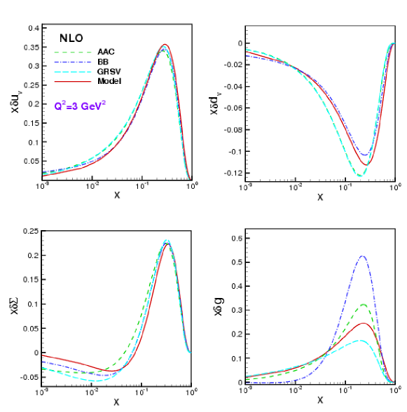
Figure 1: Polarized parton distributions in the proton at $Q^{2}=3\;GeV^{2}$ as a function of $x$ in the NLO approximation. Dashed line is the AAC model (ISET=3)[14], long-dashed line is the GRSV model (ISET=1)[15], dashed-dotted line is the BB model (ISET=3)[16] and the solid line is from [17].

3 Polarized light quark sea in the nucleon

In spite of many attempts to consider the flavor-asymmetry of the light quark sea [33], we are interesting to determine the helicity densities for the up and down quarks and anit-up, anti-down, and strange sea quarks in the NLO approximation, using the polarized valon model. We would like to briefly comment on the assumptions about the polarized anti quark asymmetry made in the recent analysis of the HERMES data for semi-inclusive DIS [28].
In the following, Subsec. 3.1 , 3.2 are advocated to unbroken and broken light quark sea, using the improved valon model.

3.1 Unbroken scenario

In this scenario one assumes, as in most analysis of polarization data performed thus far, a flavor symmetric sea, i.e.

$$\delta\bar{u}(x,Q^{2})=\delta\bar{d}(x,Q^{2})=\delta\bar{s}(x,Q^{2})\equiv\delta\bar{q}(x,Q^{2})\;,$$ (2)

where as usual $\delta u_{sea}=\delta\bar{u}$, $\delta d_{sea}=\delta\bar{d}$, and $\delta s=\delta\bar{s}$. The adopted LO and NLO distributions can be taken from the recent analysis in [17]. We have the symmetric nucleon sea

$$\delta\bar{q}(x,Q^{2})=\frac{\delta\Sigma(x,Q^{2})-\delta u_{v}(x,Q^{2})-\delta d_{v}(x,Q^{2})}{2f}\;,$$ (3)

in which the $\Sigma$ symbol denotes $\sum_{q=u,d,s}(q+\bar{q})$. In Fig. (2) we have presented the flavor symmetric sea quark densities, $x\delta\bar{q}$, as a function of $x$ at $Q^{2}=1,2.5,5,10,20,50\;GeV^{2}$ values. These distributions were calculated in the LO and NLO approximation, using polarized valon model.

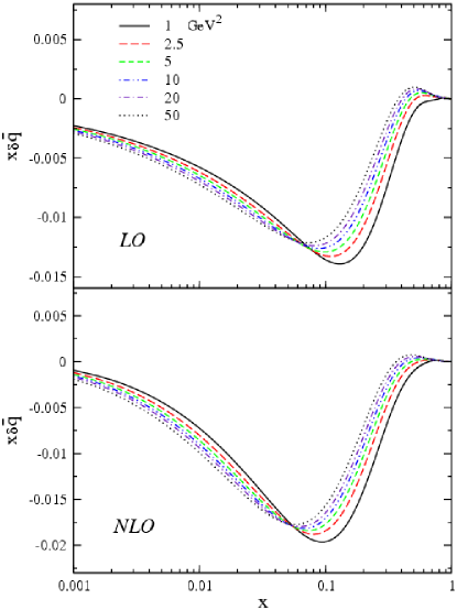
Figure 2: The flavor symmetric sea quark densities in the LO and NLO approximation as a function of $x$ and for some different values of $Q^{2}$.

By using polarized sea quark distribution and having polarized valence quark distribution, we can obtain the contributions of $\delta q(x,Q^{2})=\delta q_{v}(x,Q^{2})+\delta\bar{q}(x,Q^{2})$. In Fig. (3), we used the polarized valon model [17] and presented the $u$ and $d$ helicity quark distributions, $x\delta{u(x,Q^{2})}$ and $x\delta{d(x,Q^{2})}$ at $Q^{2}=2.5Gev^{2}$ as a function of $x$. This result was also compared with some other theoretical models in the flavor symmetric case [14-16].

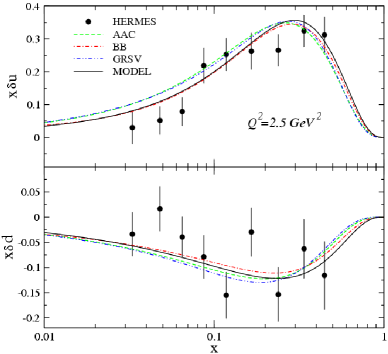
Figure 3: The $u$ and $d$ quark helicity distributions, $x\delta u(x,Q^{2})$ and $x\delta d(x,Q^{2})$, evaluated at a common value of $Q^{2}=2.5GeV^{2}$ as a function of $x$ in the flavor symmetric case. The dashed line is the AAC model (ISET=3)[14], dashed-dotted-dotted line is the GRSV model (ISET=1)[15], dashed-dotted line is the BB model (ISET=3)[16] and the solid line is from [17].

3.2 Broken scenario

We assume here $\delta\bar{u}(x,Q^{2})\neq\delta\bar{d}(x,Q^{2})\neq\delta\bar{s}(x,Q^{2})$, i.e. a broken flavor symmetry as motivated by the situation in the corresponding unpolarized case [36]. Present polarization data provide detailed and reliable information concerning flavor symmetry breaking and therefore there is enough motivation to study and utilize antiquark distributions extracted via the phenomenological ansatz.

To study the asymmetric nucleon sea we refer to an input scale $Q^{2}_{0}=1\;GeV^{2}$. In this situation we can use the Pauli-blocking relation [37] for the unpolarized and polarized antiquark distributions as

$$\frac{\bar{d}(x,Q^{2}_{0})}{\bar{u}(x,Q^{2}_{0})}=\frac{{u}(x,Q^{2}_{0})}{{d}(x,Q^{2}_{0})}\;,$$ (4)

and

$$\frac{\delta\bar{d}(x,Q^{2}_{0})}{\delta\bar{u}(x,Q^{2}_{0})}=\frac{\delta{u}(x,Q^{2}_{0})}{\delta{d}(x,Q^{2}_{0})}\;.$$ (5)

These equations are essential to study the flavor asymmetry of the unpolarized and polarized light sea quark distributions which imply that $u>d$ and consequently will determine $\bar{u}<\bar{d}$ and so on. This is in accordance with the suggestion of Feynman and Field This is correspond to the suggestion of Feynman and Field [34] that, since there are more $u$- than $d$–quarks in the proton, $u\bar{u}$ pairs in the sea are suppressed more than $d\bar{d}$ pairs by the exclusion principle. These two relations require obviously the idealized situation of maximal Pauli-blocking and hold approximately in some effective field theoretic models [33].

The flavor-broken light sea distributions are modeled in perfect and interesting way by Glück and et al.  in [38]. In that paper it was trying to use pauli-blocking ansatz and the introduction a breaking function at $Q^{2}=Q^{2}_{0}$, the valance and sea quark distributions were improved. Through this model, the necessary information about the broken symmetry of sea quark distributions has been obtained.

3.3 Asymmetric polarized valon distributions

Here we are trying to use the same strategy as in subsection 3.2 to break the polarized valon distributions which calculated in [17]. Let us begin from the definition of polarized valon distribution functions

$$\left\{\begin{array}[]{ll}\delta G_{j}(y)=\delta{\cal{W}}_{j}(y)\times G_{j}(y)&{\rm for\;non-singlet\;case\;,}\\ \delta G^{{}^{\prime}}_{j}(y)=\delta{\cal{W}}^{{}^{\prime}}_{j}(y)\times G_{j}(y)&{\rm for\;singlet\;case}\;,\end{array}\right.$$ (8)

where

$$\delta{\cal{W}}_{j}(y)=N_{j}y^{\alpha_{j}}(1-y)^{\beta_{j}}(1+\gamma_{j}y+\eta_{j}y^{0.5})\;,$$ (9)

the subscript $j$ refers to $U$ and $D$-valons. The motivation for choosing this functional form is that the low-$y$ behavior of the valon densities is controlled by the term $y^{\alpha_{j}}$ while that at the large-$y$ values is controlled by the term $(1-y)^{\beta_{j}}$. The remaining polynomial factor accounts for the additional medium-$y$ values. For $\delta{\cal{W}}^{{}^{\prime}}_{j}(y)$ in Eq.(6) we choose the following form

$$\delta{\cal{W}}^{{}^{\prime}}_{j}(y)=\delta{\cal{W}}_{j}(y)\times\sum_{m=0}^{5}{\cal A}_{m}y^{\frac{m-1}{2}}\;.$$ (10)

The extra term in the above equation, ($\sum$ term), serves to control the behavior of the singlet sector at very low-$y$ values in such a way that we can extract the sea quark contributions. Moreover, the functional form for $\delta{\cal{W}}$ and $\delta{\cal{W}}^{{}^{\prime}}$ give us the best fitting $\chi^{2}$ value[17].

Consequently we can obtain all flavor asymmetric quark distributions in the valon model frame work. The flavor-asymmetric and flavor-symmetric valon distributions are denoted by $\delta\widetilde{G}$ and $\delta G$ respectively. Since the valon distributions play the role of quark distributions at low value of $Q^{2}$, so we can define a breaking function as in [38] to determine broken polarized valon distributions from unbroken ones. These distributions are related to each other as

$$2\delta\widetilde{G}_{U}(y)\equiv 2\delta G_{U}(y)-\Theta(y)\;,$$

$$\delta\widetilde{G}_{D}(y)\equiv\delta G_{D}(y)+\Theta(y)\;,$$ (11)

here $\Theta$ is called ‘Breaking’ function and the factor 2 indicates the existence of two $U$-valons. As we will see, to determine this function, we need to obtain the contributions of sea quarks in the improved valon model framework.

By using [17] we can get the following expressions for the polarized parton distributions in a proton:

$$\delta u_{v}(x,Q^{2}) = 2\int_{x}^{1}\delta f^{NS}(\frac{x}{y},Q^{2})\;\delta G_{U}(y)\;\frac{dy}{y}\;,$$

$$\delta d_{v}(x,Q^{2}) = \int_{x}^{1}\delta f^{NS}(\frac{x}{y},Q^{2})\;\delta G_{D}(y)\;\frac{dy}{y}\;,$$

$$\delta\Sigma(x,Q^{2}) = \int_{x}^{1}\delta f^{S}(\frac{x}{y},Q^{2})\left(2\;[\delta G^{{}^{\prime}}_{U}(y)+\delta G^{{}^{\prime}}_{D}(y)]\right)\;\frac{dy}{y}\;,$$

here $\delta f^{NS}$ and $\delta f^{S}$ indicate the Non-singlet and Singlet parton distributions inside the valon. To obtain the $z$-dependence of parton distributions, $\delta f^{NS,\;S}(z=\frac{x}{y},Q^{2})$, from the $n-$dependent exact analytical solutions in the Mellin-moment space, one has to perform a numerical integral in order to invert the Mellin-transformation [17].

At the input scale $Q_{0}^{2}=1\;GeV^{2}$, $\delta f^{NS}$ and $\delta f^{S}$ behave like the delta function and consequently $\delta u_{v}(x,Q_{0}^{2})$ is approaching to $2\delta G_{U}$ and similarly $\delta d_{v}(x,Q_{0}^{2})$ to $\delta G_{D}$. Finally $\delta\Sigma(x,Q_{0}^{2})$ will be equal $2\delta G_{U}^{\prime}(y)+\delta G_{D}^{\prime}(y)$. We should notice that in this scale, $x$-space is equal to $y$-space. Now the first term in the numerator of Eq. (3) is equal to $2\delta G_{U}^{\prime}(y)+\delta G_{D}^{\prime}(y)$ and the rest two terms to $2\delta G_{U}(y)+\delta G_{D}(y)$, therefor the Eq. (3) at $Q^{2}=Q_{0}^{2}$ can be expressed as a combination of $\delta G_{j}$ and $\delta G_{j}^{\prime}$ in the following form

$$\delta G^{\bar{q}}\equiv\frac{1}{2f}\sum_{j}(\delta G_{j}^{\prime}-\delta G_{j}),$$ (13)

where $j$ denotes the $U,U,D$-valons. Here $\delta G^{\bar{q}}$ denotes to polarized see quark contribution at $Q^{2}=Q_{0}^{2}$ which is arising out from symmetric valon distributions.
In order to determine breaking function, we need the following relations

$$\delta G^{\bar{u}}(y)\equiv\delta G^{\bar{q}}(y)+\frac{\Theta(y)}{2}\;,$$

$$\delta G^{\bar{d}}(y)\equiv\delta G^{\bar{q}}(y)-\frac{\Theta(y)}{2}\;,$$ (14)

where $\delta G^{\bar{u}}$ and $\delta G^{\bar{d}}$ indicate polarized see quark contributions which are obtained from asymmetric valon distributions.

In the valon model framework, Eq. (5) can be considered as

$$\frac{\delta G^{\bar{d}}(y)}{\delta G^{\bar{u}}(y)}=\frac{2\delta\widetilde{G}_{U}(y)+{\delta G^{\bar{u}}(y)}}{\delta\widetilde{G}_{D}(y)+{\delta G^{\bar{d}}(y)}}\;.$$ (15)

On the other hand from Eq. (14) we have

$$\frac{\delta G^{\bar{d}}(y)}{\delta G^{\bar{u}}(y)}=\frac{\delta G^{\bar{q}}(y)-\frac{\Theta(y)}{2}}{\delta G^{\bar{q}}(y)+\frac{\Theta(y)}{2}}\;.$$ (16)

So by using Eqs. (15,16) and inserting the related functions from Eq. (11) we arrive at

$$\frac{\delta G^{\bar{q}}-\frac{\Theta}{2}}{\delta G^{\bar{q}}+\frac{\Theta}{2}}=\frac{2\delta{G}_{U}-\Theta+\delta G^{\bar{q}}+\frac{\Theta}{2}}{\delta{G}_{D}+\Theta+\delta G^{\bar{q}}-\frac{\Theta}{2}}\;.$$ (17)

The breaking function can be extracted from Eq. (17) as follows

$$\Theta\equiv-2\delta G^{\bar{q}}\;\frac{2\delta G_{U}-\delta G_{D}}{2\delta G_{U}+\delta G_{D}}\;.$$ (18)

It is obvious that the combination of Eqs.(9,11) will lead to the following constrains

$$2\delta\widetilde{G}_{U}(y)+2\delta G^{\bar{u}}(y)=2\delta{G}_{U}(y)+2\delta G^{\bar{q}}(y)\;,$$

$$\delta\widetilde{G}_{D}(y)+2\delta G^{\bar{d}}(y)=\delta{G}_{D}(y)+2\delta G^{\bar{q}}(y)\;,$$

$$2\delta\widetilde{G}_{U}(y)+\delta\widetilde{G}_{D}(y)=2\delta{G}_{U}(y)+\delta{G}_{D}(y)\;,$$ (19)

in which, for instance, the first equation in Eq. (17) has been obtained from the combining of first equation in Eq. (10) with the first equation in Eq. (12). Using these constrains, it will be seen that the first moment of $g_{1}^{p}$ will not change in the broken sea scenario.

Since the polarized valon and sea quark distributions are known in [17], by substituting them in Eq. (18), the breaking function $\Theta$ can be simply parameterized in the LO and NLO approximations as

$$y\Theta_{LO}(y)=0.060y^{0.496}(1-y)^{7.735}(1+10.443y+3.371y^{2}-5.759y^{3})\;,$$ (20)

$$y\Theta_{NLO}(y)=0.192y^{0.619}(1-y)^{7.228}(1-0.037y-0.310y^{2}+1.273y^{3})\;,$$ (21)

which needed for performing the $Q^{2}$-evolution in the $x$-space with using the convolution integral.

If we back to Eq. (1) and substitute the related broken valon distributions, we will be able to obtain the $Q^{2}$ dependent of the parton distribution in broken scenario. Our results for the polarized parton distributions at $Q^{2}=5\;GeV^{2}$ are presented in Fig. (4). In this figure a comparison between the distributions in the LO (broken scenario) and NLO approximations (broken and unbroken scenario) has been done.

It was assumed that $\delta s=\delta{\overline{s}}\equiv\delta\overline{q}$. We also did not consider any asymmetry for the strange quark and gluon distributions. In Fig. (5), the quark helicity distributions $x\delta q(x,Q^{2})$ for $q=u,d,\bar{u},\bar{d}$ and $s$ are shown at value of $Q^{2}=2.5\;GeV^{2}$ in the LO and NLO approximation. We have also compared in this figure our model with recent HERMES [28] data and GRSV model[15].

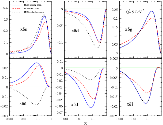
Figure 4: The LO (broken scenario) and NLO approximations (broken and unbroken scenario), for polarized parton distributions at $Q^{2}=5\;GeV^{2}$. The line is the NLO distributions in broken scenario , the dotted line is the NLO distributions in unbroken scenario and the dashed line is the LO distributions in broken scenario.

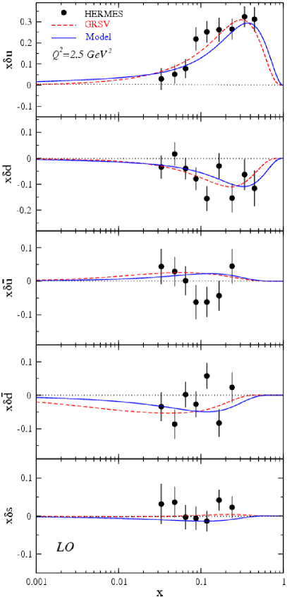
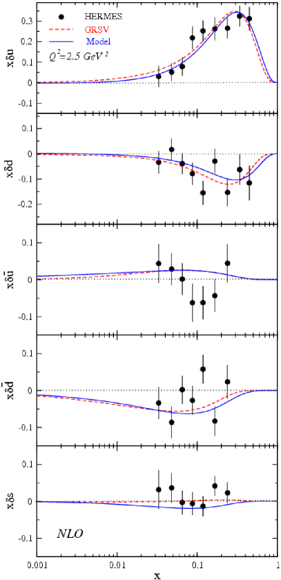
Figure 5: The quark helicity distributions $x\delta q(x,Q^{2})$ evaluated at value of $Q^{2}=2.5\;GeV^{2}$ as a function of $x$ in the LO and NLO approximations. The dashed line is the GRSV model [15](ISET=2 for the NLO and ISET=4 for the LO approximation) and the solid line is our model.

After calculating $x\delta\bar{u}$ and $x\delta\bar{d}$ for instance at $Q^{2}=2.5\;GeV^{2}$, we can obtain the results of $x\delta\bar{u}-x\delta\bar{d}$. In Fig. (6), we have presented this function in the broken scenario evaluated in the LO, NLO approximations and compared it with the recent HERMES [28] data and GRSV model[15].

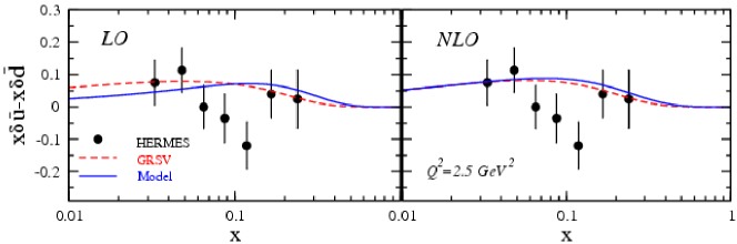
Figure 6: The flavor asymmetry in the helicity densities of the light sea evaluated at $Q^{2}=2.5GeV^{2}$. The dashed line is the GRSV model [15](ISET=2 for the NLO and ISET=4 for the LO approximation) and the solid line is our model.

4 Moments of helicity distributions

In this section we study the first moment of the polarized parton distributions in the broken scenario. The total helicity of a specific parton $f$ is given by the first ($n=1$) moment

$$\Delta f(Q^{2})\equiv\int_{0}^{1}dx\,\delta f(x,Q^{2})\,.$$ (22)

The contribution of various polarized partons in a valon are calculable and by computing their first moment, the spin of the proton can be computed. In the framework of QCD the spin of the proton can be expressed in terms of the first moment of the total quark and gluon helicity distributions and their orbital angular momentum, i.e.

$$\frac{1}{2}=\frac{1}{2}\Delta\Sigma(Q^{2})+\Delta g(Q^{2})+L_{z}(Q^{2})\;,$$ (23)

which is called the helicity sum rule. Here $L_{z}$ refers to the total orbital contribution of all (anti)quarks and gluons to the spin of the proton.

The contributions of $\delta\Sigma(x,Q^{2})$ and $\delta g(x,Q^{2})$ to the spin of proton can be calculated as in following. The singlet contributions form $j$-valon in a proton can be extracted via [17]

$$\delta\Sigma^{j}(x,Q^{2}) = \int_{x}^{1}\delta f^{S}(\frac{x}{y},Q^{2})[\delta{\cal{W}}^{{}^{\prime}}_{j}(y)\times G_{j/p}(y)]\frac{dy}{y}\;,$$ (24)

and the gluon distribution for $j$-valon is

$$\delta g^{j}(x,Q^{2}) = \int_{x}^{1}\delta f^{gq}(\frac{x}{y},Q^{2})[\delta{\cal{W}}_{j}(y)\times G_{j/p}(y)]\frac{dy}{y}\;,$$ (25)

where the functional form for $\delta{\cal{W}}_{j}(y)$ and $\delta{\cal{W}}^{{}^{\prime}}_{j}(y)$ have been defined in Subsec. 3.3.
Using Eq. (22) and Eqs. (24,25) we can arrive at the first moments of the related parton distributions as follows

$$\Delta\Sigma^{j}(Q^{2}) = \int_{0}^{1}\delta\Sigma^{j}(x,Q^{2})dx\;,$$ (26)

$$\Delta g^{j}(Q^{2}) = \int_{0}^{1}\delta g^{j}(x,Q^{2})dx\;.$$ (27)

The resulting total quark and gluon helicity for a $U$-valon is

$$\frac{1}{2}\Delta\Sigma^{U}(Q^{2})+\Delta g^{U}(Q^{2})\;,$$ (28)

and for $D$-valon

$$\frac{1}{2}\Delta\Sigma^{D}(Q^{2})+\Delta g^{D}(Q^{2})\;.$$ (29)

Since each proton involves 2 $U$-valons and one $D$-valon, the total quark and gluon helicity for the proton is

$$2\left(\frac{1}{2}\Delta\Sigma^{U}(Q^{2})+\Delta g^{U}(Q^{2})\right)+\frac{1}{2}\Delta\Sigma^{D}(Q^{2})+\Delta g^{D}(Q^{2})=\frac{1}{2}\Delta\Sigma(Q^{2})+\Delta g(Q^{2})\;.$$ (30)

The proton’s spin is carried almost entirely by the total helicities of quarks and gluons and at $Q_{0}^{2}$ in the NLO approximation is given by

$$\frac{1}{2}\Delta\Sigma+\Delta g\simeq 0.637,$$ (31)

which is calculated in the NLO approximation at $Q_{0}^{2}$ value. This amount is equal to the unbroken scenario result [17], and thus a negative orbital contribution $L_{z}(\simeq-0.1373$) is required at the low input scales in order to comply with the sum rule Eq. (23). It is intuitively appealing that the non perturbative orbital (angular momentum) contribution to the helicity sum rule Eq. (23) is noticeable because of hard radiative effects which give rise to sizeable orbital components due to the increasing transverse momentum of the partons.

By using the results of Sec. 3 for the polarized parton distributions in broken scenario and the definition of first moment for these distributions as defined in Eq. (22), the numerical results for the first moments are calculable. Our NLO results are summarized in Table ${\bf I}$ at some typical values of $Q^{2}$.

$Q^{2}(GeV^{2})$	$\Delta u_{v}$	$\Delta d_{v}$	$\Delta\overline{u}$	$\Delta\overline{d}$	$\Delta s=\Delta\overline{s}$	$\Delta g$	$\Delta\Sigma$	$\Gamma_{1}^{p}$
$1$	0.5760	- 0.0280	0.0907	-0.2139	-0.0615	0.5480	0.1786	0.1214
$2.5$	0.5731	-0.0269	0.0901	-0.2145	-0.0621	0.7417	0.1732	0.1238
$5$	0.5716	-0.0264	0.0899	-0.2148	-0.0624	0.8737	0.1706	0.1249
$10$	0.5706	-0.0260	0.0897	-0.2150	-0.0626	0.9986	0.1688	0.1258

Table I First moments (total polarizations) of polarized parton densities and $g_{1}^{p}(x,Q^{2})$, as defined in Eq. (22) and in the flavor-broken scenario.

5 Orbital angular momentum

The fundamental program in high energy spin physics focuses on the spin structure of the nucleon. The nucleon spin can be decomposed conceptually into the spin of its constituents according to helicity sum rule. In last section we analyzed $\Delta\Sigma$ and $\Delta g$ for each $Q^{2}$ value from polarized valon model. Here we calculate the total orbital angular momenta of quarks and gluons, $L_{z}(Q^{2})\equiv L_{z}^{q}(Q^{2})+L_{z}^{G}(Q^{2})$. We know that two places where the orbital angular momentum plays a role. One is the compensation of the growth of $\Delta G$ with $Q^{2}$ by the angular momentum of the quark-gluon pair. The other is the reduction of the total spin component $\Delta\Sigma$ due to the presence of the quark transverse momentum in the lower component of the Dirac spinor which is traded with the quark orbital angular momentum.

The evolution of the quark and gluon orbital angular momenta was first discussed by Ratcliffe [39]. A complete leading-log evolution equation have been derived by Ji, Tang and Hoodbhoy [35]:

$$\frac{d}{dt}\left(\begin{array}[]{l}L_{z}^{q}\\ L_{z}^{G}\end{array}\right)=\frac{\alpha_{s}(t)}{2\pi}\left(\begin{array}[]{ll}-\frac{4}{3}C_{F}&\frac{n_{f}}{3}\\ \frac{4}{3}C_{F}&-\frac{n_{f}}{3}\end{array}\right)\left(\begin{array}[]{l}L_{z}^{q}\\ L_{z}^{G}\end{array}\right)+\frac{\alpha_{s}(t)}{2\pi}\left(\begin{array}[]{ll}-\frac{2}{3}C_{F}&\frac{n_{f}}{3}\\ -\frac{5}{6}C_{F}&-\frac{11}{2}\end{array}\right)\left(\begin{array}[]{l}\Delta\Sigma\\ \Delta G\end{array}\right),$$ (42)

with the solutions

$$L_{z}^{q}(Q^{2})=-{1\over 2}\Delta\Sigma+{1\over 2}\,{3n_{f}\over 16+3n_{f}}+f(Q^{2})\left(L_{z}^{q}(Q^{2}_{0})+{1\over 2}\Delta\Sigma-{1\over 2}\,{3n_{f}\over 16+3n_{f}}\right),$$ (43)

$$L_{z}^{G}(Q^{2})=-\Delta G(Q^{2})+{1\over 2}\,{16\over 16+3n_{f}}+f(Q^{2})\left(L_{z}^{G}(Q^{2}_{0})+\Delta G(Q^{2}_{0})-{1\over 2}\,{16\over 16+3n_{f}}\right),$$

where

$$f(Q^{2})=\left({\alpha(Q^{2})\over\alpha(Q^{2}_{0})}\right)^{{32+6n_{f}\over 33-2n_{f}}}\;,$$ (45)

and $\Delta\Sigma$ is $Q^{2}$ independent to the leading-log approximation. We see that the growth of $\Delta G$ with $Q^{2}$ is compensated by the gluon orbital angular momentum, which also increases like $\ln Q^{2}$ but with opposite sign.

If we know the total value of quark and gluon orbital angular momentum at $Q^{2}_{0}$, then according to Eqs. (43,5), $L_{z}^{q}(Q^{2})+L_{z}^{G}(Q^{2})$ can be computed at each value of $Q^{2}$. By evaluating Eq. (30) and using the sum rule, Eq. (23) at $Q_{0}^{2}$, we can obtain the total quark and gluon orbital angular momentum at $Q^{2}_{0}$. By adding Eqs. (43,5) and inserting $L_{z}^{q}(Q_{0}^{2})+L_{z}^{G}(Q_{0}^{2})$ in the additive equation, the $Q^{2}$-evolution of total quark and gluon orbital angular momentum will be accessible. The result for $L_{z}^{q}(Q^{2})+L_{z}^{G}(Q^{2})$ in range of $1\leq Q^{2}(GeV^{2})\leq 1000$ has been depicted in Fig. (7) .

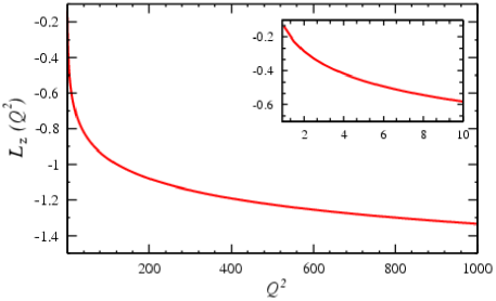
Figure 7: The $Q^{2}$ evolution of $L_{z}$ in the LO approximation.

On the other hand, we can directly obtain $L_{z}(Q^{2})$, using the helicity sum rule Eq. (23). In this case the $\frac{1}{2}\Delta\Sigma(Q^{2})$ and $\Delta g(Q^{2})$ are known from polarized valon model in the LO and NLO approximation. By having different values of these two functions at some values of $Q^{2}$, inserting them in the related sum rule and fitting over the calculated data points for $L_{z}(Q^{2})$, the functional form for $L_{z}(Q^{2})$ will be obtained in these two approximations. The result for $L_{z}(Q^{2})$ in the LO approximation, computed from Eqs. (43,5), is completely consistent with the one from the sum rule in Eq. (23). If we use from the data points for $L_{z}(Q^{2})$, arising out from the Eq. (23) but in the NLO approximation, we will obtain the functional form $L_{z}(Q^{2})=-5.10+4.96(Q^{2})^{-0.04}$. Since the obtained results for $L_{z}(Q^{2})$ in the LO approximation, using evolution equations or fitting procedure, are in agreement with each other, so it will be possible to say that in the NLO approximation the obtained fitting functional form for $L_{z}(Q^{2})$ will be correspond to what will be resulted from evolution of this quantity.

6 Conclusions

Polarized deep inelastic scattering (DIS) is a powerful tool for the investigation of the nucleon spin structure. Experiments on polarized deep inelastic lepton-nucleon scattering started in the middle 70s. Measurements of cross section differences with the longitudinally polarized lepton beam and nucleon target determine the polarized nucleon structure functions $g_{1}(x,Q^{2})$. During the period of 1988-1993, theorists tried to resolve the proton spin enigma and seek explanations for the measurements of first moment of proton structure function, $\Gamma^{p}_{1}$. These moments were produced by European Muon Collaboration (EMC), assuming the validity of the data at small $x$ and of the extrapolation procedure to the unmeasured small $x$ region.

The determination of the polarized proton content of the nucleon via measurements of the inclusive structure function $g_{1}(x,Q^{2})$ dose not provide detailed information concerning the flavor structure of these distributions. In particular the flavor structure of the anti-quark (sea) distributions is not fixed and one needs to resort to semi-inclusive deep in elastic hadron production for this propose. The resulting anti-quark distributions $\delta\bar{q}$ are, however, not reliably determined by this method for the time being due to their dependence on the rather poorly known quark fragmentation function at low scales. Since now there are enough experimental date from semi-inclusive DIS experiments at DESY (HERMES), we followed the strategy of [38] to break see quark distributions but in frame work of polarized valon model. The comparison of our obtained results for $\delta\bar{u}(x,Q^{2}),\delta\bar{d}(x,Q^{2})$ and $\delta\bar{s}(x,Q^{2})$ with the only available GRSV model [15] and experimental date from HERMES group indicate a very good agreement with them specially for strange sea quark while we expect to have a negative strange-quark polarization. Since the total contribution of sea quarks is remaining constant in two unbroken and broken scenario, the first moment of $g_{1}^{p}$, $\Gamma_{1}^{p}$, will be fixed, as is expected.

If we back again to spin nucleon subject, we see that the measurements by the EMC first indicated that only a small fraction of the nucleon spin is due to the spin of the quarks[19]. Thus it refers to existence of other components in performing the spin of nucleon. In fact the nucleon spin can be decomposed conceptually into the angular momentum contributions of its constituents according to the Eq. (23) where the rest two terms of this equation give the contributions to the nucleon spin from the helicity distributions of the quark and gluon respectively. The angular momentum contribution has been calculated in the LO approximation, using its $Q^{2}$ evolution in Eqs. (43,5). If we know the parton distributions in the NLO approximation, which obviously are known using polarized valon model [17], then it will possible to calculate the $\Delta\Sigma$ and $\Delta g$ contributions and finally using the helicity sum rule, to compute the $L_{z}$ contribution.

Extracting the $L_{z}^{q}(Q^{2})$ and $L_{z}^{g}(Q^{2})$ which refer to separate contributions of quark and gluon angular momentum, using the polarized valon model, would also be valuable and challenging. We hope to report on this subject in further publications.

The numerical data for the polarized quark distributions in unbroken and broken scenarios are available by electronic mail from $Alinaghi.Khorramian@cern.ch$.

7 Acknowledgments

We are thankful to R. C. Hwa for his useful comments to help us in constructing the unbroken polarized valon model. The authors are indebted to M. Mangano to read the manuscript. We acknowledge the Institute for Studies in Theoretical Physics and Mathematics (IPM) for financially supporting this project.

References

- [1] M. Glück, E. Reya, M. Stratmann, and W. Vogelsang, Phys. Rev. D53, 4775 (1996).
- [2] T. Gehrmann and W.J. Stirling, Phys. Rev. D53, 6100 (1996).
-
[3]
R.D. Ball, S. Forte, and G. Ridolfi, Phys. Lett.
B378, 255 (1996);
G. Altarelli, R.D. Ball, S. Forte, and G. Ridolfi, Nucl. Phys. B496, 337 (1997); Acta Phys. Pol. B29, 1145(1998). - [4] K. Abe et al., SLAC-E154 Collab., Phys. Lett. B405, 180 (1997).
- [5] B. Adeva et al., CERN-SM Collab., Phys. Rev. D58, 112002 (1998).
- [6] C. Bourrely, F. Buccella, O. Pisanti, P. Santorelli, and J. Soffer, Prog. Theor. Phys. 99, 1017 (1998).
- [7] D. de Florian, O.A. Sampayo, and R. Sassot, Phys. Rev. D57, 5803 (1998).
- [8] E.A. Leader, A.V. Sidorov, and D.B. Stamenov, Int. J. Mod. Phys. A13, 5573 (1998); Phys. Rev. D58, 114028 (1998); Phys. Lett. B445, 232 (1998); B462, 189 (1999); Phys. Lett. B488, 283 (2000).
- [9] L.E. Gordon, M. Goshtasbpour, and G.P. Ramsey, Phys. Rev. D58, 094017 (1998).
- [10] S. Incerti and F. Sabatie, SLAC-E154/155 Collab., CEA–Saclay PCCF-RI-9901 (1999).
-
[11]
S. Tatur, J. Bartelski, and M. Kurzela, Acta. Phys. Pol. B31,
647 (2000);
J. Bartelski and S. Tatur, hep–ph/0004251 (2000). - [12] D.K. Ghosh, S. Gupta, and D. Indumathi, Phys. Rev. D62, 094012 (2000).
- [13] D. de Florian and R. Sassot, Phys. Rev. D62, 094025 (2000).
- [14] Y. Goto et al., Asymmetry Analysis Collab., Phys. Rev. D62, 034017 (2000).
- [15] M. Glück, E. Reya, M. Stratmann and W. Vogelsang, Phys. Rev. D63(2001) 094005.
- [16] J. Blümlein, H. Böttcher, Nucl. Phys. B636(2002) 225.
- [17] Ali N. Khorramian, A. Mirjalili, S. Atashbar Tehrani, JHEP 0410, 062 (2004), hep-ph/0411390.
-
[18]
SLAC–Yale E80 Collaboration, M.J. Alguard et al.,
Phys. Rev. Lett. 37, 1261 (1976); G. Baum
et al., ibid. 45, 2000 (1980);
SLAC–Yale–E130 Collaboration, G. Baum et al., Phys. Rev. Lett. 51, 1135 (1983). - [19] CERN–EM Collaboration, J. Ashman et al., Phys. Lett. B206, 364 (1988); Nucl. Phys. B328, 1 (1989).
- [20] CERN–SM Collaboration, B. Adeva et al., Phys. Rev. D58, 112001 (1998).
- [21] SLAC–E143 Collaboration, K. Abe et al., Phys. Rev. D58, 120003 (1998 ).
- [22] SLAC–E142 Collaboration, P.L. Anthony et al., Phys. Rev. D54, 6620 (1996).
- [23] DESY–HERMES Collaboration, K. Ackerstaff et al., Phys. Lett. B404, 383 (1997).
- [24] DESY–HERMES Collaboration, A. Airapetian et al., Phys. Lett. B442, 484 (1998).
- [25] SLAC–E154 Collaboration, K. Abe et al., Phys. Rev. Lett. 79, 26 (1997).
- [26] SLAC-E155 Collaboration, P.L. Anthony et al., Phys. Lett. B463, 339 (1999).
- [27] SLAC–E155 Collaboration, P.L. Anthony et al., SLAC–PUB–7994, July 2000 T/E (hep–ph/0007248).
-
[28]
HERMES Collaboration, A. Airapetian et al.,
Phys. Rev. Lett. 92, 012005 (2004);
HERMES Collaboration, A. Airapetian et al., Phys. Rev. D71, 012003 (2005). - [29] R. C. Hwa, Phys. Rev. D22,(1980) 759.
- [30] R. C. Hwa, Phys. Rev. D22,(1980) 1593.
- [31] R. C. Hwa and M. S. Zahir, Phys. Rev. D23, (1981) 2539.
- [32] R. C. Hwa and C. B. Yang, Phys. Rev. C66 (2002) 025204; R. C. Hwa and C. B. Yang, Phys. Rev. C66 (2002) 025205.
- [33] S. Kumano, Phys. Rep. 303, 183 (1998), and references therein.
- [34] R.D. Field and R.P. Feynman, Phys. Rev. D15, 2590 (1977).
- [35] X. Ji, J. Tang, and P. Hoodbhoy, Phys. Rev. Lett. 76, 740 (1996).
- [36] F. Arash and Ali N. Khorramian, Phys. Rev. C67 (2003) 045201; hep-ph/0303031.
- [37] M. Glück, E. Reya, Mod. Phys. Lett. A15,(2000) 883; hep-ph/0002182.
- [38] M. Glück, A. Hartl, and E. Reya, Eur. Phys. J. C19, 77 (2001).
- [39] P. Ratcliffe, Phys. Lett. B192, 180 (1987).