Mass and width of the $\,\sigma$

Abstract

Contribution to the proceedings of MESON 2006 (Krakow)

I report on recent work done in collaboration with Irinel Caprini and Gilberto Colangelo CCL . We observe that the Roy equations lead to a representation of the $\pi\pi$ scattering amplitude that exclusively involves observable quantities, but is valid for complex values of $s$. At low energies, this representation is dominated by the contributions from the two subtraction constants, which are known to remarkable precision from the low energy theorems of chiral perturbation theory. Evaluating the remaining contributions on the basis of the available data, we demonstrate that the lowest resonance carries the quantum numbers of the vacuum and occurs in the vicinity of the threshold. Although the uncertainties in the data are substantial, the pole position can be calculated quite accurately, because it occurs in the region where the amplitude is dominated by the subtractions. The calculation neatly illustrates the fact that the dynamics of the Goldstone bosons is governed by the symmetries of QCD.

Pions play a crucial role whenever the strong interaction is involved at low energies – the Standard Model prediction for the muon magnetic moment provides a good illustration. The present talk concerns the remarkable theoretical progress made in low energy pion physics in recent years. I concentrate on work based on dispersion theory CCL , but also show some lattice results, obtained with quark masses that are small enough for a controlled extrapolation to the values of physical interest to be within reach. The low energy precision measurements E865 ; DIRAC ; NA48 are consistent with the predictions and even offer a stringent test for one of these.

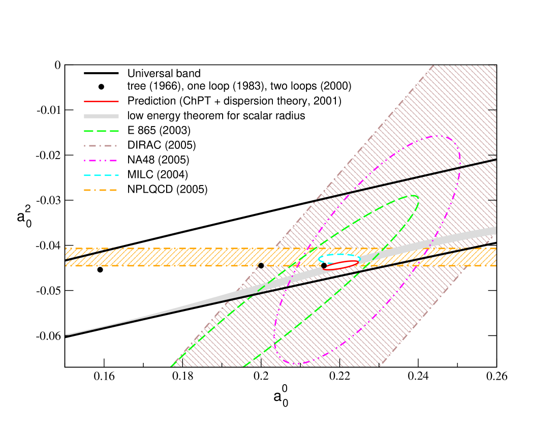
Figure 1: $S$ wave scattering lengths.

From the point of view of dispersion theory, $\pi\pi$ scattering is particularly simple: the $s$-, $t$- and $u$-channels represent the same physical process. As a consequence, the real part of the scattering amplitude can be represented as a dispersion integral over the imaginary part and the integral exclusively extends over the physical region Roy . The representation involves two subtraction constants, which may be identified with the $S$-wave scattering lengths $a_{0}^{0},a_{0}^{2}$. The projection of the amplitude on the partial waves leads to a dispersive representation for these, the Roy equations.

The pioneering work on the physics of the Roy equations was carried out more than 30 years ago MP . The main problem encountered at that time was that the two subtraction constants occurring in these equations were not known. These constants dominate the dispersive representation at low energies, but since the data available at the time were consistent with a very broad range of $S$-wave scattering lengths, the Roy equation analysis was not conclusive.

The insights gained by means of $\chi$PT thoroughly changed the situation. The corrections to Weinberg’s low energy theorems Weinberg 1966 for $a_{0}^{0},a_{0}^{2}$ (left dot in Fig.1) have been worked out to first non-leading order GL (middle dot) and those of next-to-next-to leading order are also known BCEGS (dot on the right). Very accurate predictions for the scattering lengths are obtained by matching the chiral and dispersive representations in the interior of the Mandelstam triangle CGL (small ellipse). The lattice results of the MILC collaboration MILC also yield an estimate for the scattering lengths. Using their values for the coupling constants $L_{4},L_{5},L_{6},L_{8}$ of the effective chiral lagrangian and neglecting two loop effects, we arrive at the one standard deviation contour indicated by the small dashed ellipse. The horizontal band represents the value of the scattering length $a_{0}^{2}$ obtained by the NPLQCD collaboration Beane .

The plot shows that $\pi\pi$ scattering is one of the very rare hadronic processes where theory is ahead of experiment: the two large ellipses and the tilted band indicate the results obtained on the basis of experiments done at Brookhaven E865 and CERN DIRAC ; NA48 . Possibly, the error estimates attached to the lattice results are too optimistic and the analysis of the $K\rightarrow 3\pi$ data also requires further study, but it is fair to say that all of the published results confirm the theoretical predictions.

In the following, I focus on the results obtained on this basis for the low energy properties of the isoscalar $S$-wave. The corresponding $S$-matrix element, $S_{0}^{0}=\eta_{0}^{0}\exp 2\,i\,\delta_{0}^{0}$, is related to the partial wave amplitude $t_{0}^{0}$ by

$$S_{0}^{0}(s)=1+2\,i\,\rho(s)\,t_{0}^{0}(s)\,,\hskip 20.00003pt\rho(s)=\sqrt{1-4M_{\pi}^{2}/s}\,.$$ (1)

The various phenomenological analyses are not in good agreement pheno . In fact, until ten years ago, the information about the $\sigma=f_{0}(600)$ was so shaky that this resonance was banned from the data tables. The work of Törnqvist and Roos Tornqvist and Roos resurrected it, but the estimate $M_{\sigma}-\frac{i}{2}\,\Gamma_{\sigma}=(400\div 1200)-i\,(300\div 500)$ MeV of the Particle Data Group PDG 2006 indicates that it is not even known for sure whether the lowest resonance of QCD carries the quantum numbers of the $\sigma$ or those of the $\rho$.

The positions of the poles represent universal properties of the strong interaction which are unambiguous even if the width of the resonance turns out to be large, but they concern the non-perturbative domain, where an analysis in terms of the local degrees of freedom of QCD – quarks and gluons – is not in sight. One of the reasons why the values for the pole position of the $\sigma$ quoted by the Particle Data Group cover a very broad range is that all of these rely on the extrapolation of hand made parametrizations: the data are represented in terms of suitable functions on the real axis and the position of the pole is determined by continuing this representation into the complex plane. If the width of the resonance is small, the ambiguities inherent in the choice of the parametrization do not significantly affect the result, but the width of the $\sigma$ is not small.

We have found a method that does not invoke parametrizations of the data. It relies on the following two observations:

1. The $S$-matrix has a pole on the second sheet if and only if it has a zero on the first sheet. In order to determine the pole position it thus suffices to have a reliable representation of the scattering amplitude on the first sheet.

2. The Roy equations hold not only on the real axis, but in a limited region of the first sheet. Since the pole from the $\sigma$ occurs in that region, we do not need to invent a parametrization, but can rely on the explicit representation of the amplitude provided by these equations.

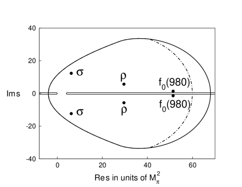
Figure 2: Domain of validity of the Roy equations.

Roy established the validity of his equations from first principles for real values of s in the interval $-4M_{\pi}^{2}<s<60M_{\pi}^{2}$. Using known results of general quantum field theory Martin book , we have demonstrated that these equations also hold for complex values of $s$, in the intersection of the relevant Lehmann-Martin ellipses CCL . The dash-dotted curve in Fig.2 shows the domain of validity that follows from axiomatic field theory, while the full line depicts the slightly larger domain obtained under the assumption that the scattering amplitude obeys the Mandelstam representation. I emphasize that the boundary does not represent a singularity of the amplitude, but merely limits the region where the Roy equations hold in the form given. Modified representations with a much larger domain of validity can be found in the work of Roy and Wanders Roy Wanders 1978 and in the references quoted therein.

For our analysis, it is essential that the dispersion integrals are dominated by the contributions from the low energy region: because the Roy equations involve two subtractions, the kernels fall off with the third power of the variable of integration. The left hand cut plays an important role here: taken by itself, the contribution from the right hand cut is sensitive to the poorly known high energy behaviour of the imaginary parts, but taken together with the one from the left hand cut, the high energy tails cancel. In this connection, I note that most pole determinations assume that the left hand cut can be neglected FN Zhou . Since the distance between the pole and the left hand cut is not large, this assumption is difficult to justify.

The Roy equations thus provide us with an explicit representation of the function $S^{0}_{0}(s)$ for complex values of $s$, in terms of rapidly convergent dispersion integrals over the imaginary parts of the partial waves. In connection with the determination of the pole from the $\sigma$, the most important contribution is the one from the subtraction term. The dispersion integrals over the $S$- $P$- and $D$-waves generate a correction which can be evaluated with available phase shift analyses – in particular with the one obtained by solving the Roy equations CGL . The contributions from high energies and high angular momenta can be estimated by means of the Regge representation of the scattering amplitude ACGL – these contributions barely affect the pole position.

For the central solution of the Roy equations, the function $S_{0}^{0}(s)$ contains two pairs of zeros in the domain of interest:

$$s_{\sigma}=(6.2\pm i\,12.3)\,M_{\pi}^{2}\,,\hskip 10.00002pts_{\!f_{0}}=(51.4\pm i\,1.4)\,M_{\pi}^{2}\,.$$ (2)

These are indicated in Fig.2, which may also be viewed as a picture of the second sheet – the dots then represent poles rather than zeros. For comparison, the figure also indicates the position of the zeros in $S^{1}_{1}(s)$, which characterize the $\rho$.

The higher one of the two pairs of zeros represents the well-established resonance $f_{0}(980)$, which sits close to the threshold of the transition $\pi\pi\rightarrow K\bar{K}$. The corresponding pole generates a spectacular interference phenomenon with the branch point singularity, which gives rise to a sharp drop in the elasticity. Our analysis adds little to the detailed knowledge of that structure.

The lower pair of zeros corresponds to a pole in the lower half of the second sheet at CCL

$$M_{\sigma}-\frac{i}{2}\,\Gamma_{\sigma}=\sqrt{s_{\sigma}}=441\,\rule[-1.99997pt]{0.0pt}{10.00002pt}^{+16}_{-\,8}-\,i\;272\,\rule[-1.99997pt]{0.0pt}{10.00002pt}^{+\,9}_{-12.5}\;\mbox{MeV}\,.$$ (3)

The error bars account for all sources of uncertainty. They are calculated by (a) estimating the uncertainties in the input used when solving the Roy equations and (b) following error propagation to determine the uncertainty in the result for the pole position. For details, I refer to our publication CCL .

Figure 3: Dominance of the subtraction term.

The reason why the pole position of the $\sigma$ can be calculated rather accurately is that (a) the pole occurs at low energies and (b) there, the isoscalar $S$-wave is dominated by the subtraction term. This is illustrated in Fig.3, where the real part of $t^{0}_{0}(s)$ is plotted versus $s$. The graph demonstrates that, in the region shown, the full amplitude closely follows the subtraction term. The final state interaction does generate curvature – in particular, the cusp at $s=4M_{\pi}^{2}$ is visible – but since Goldstone bosons of low momentum interact only weakly, the contributions from the dispersion integrals amount to a small correction. In the language of $\chi$PT , the dispersion integrals only show up at NLO. Moreover, at leading order, the subtraction constants are determined by the pion decay constant. Dropping the dispersion integrals and inserting the lowest order predictions for the scattering lengths, the Roy equation for the isoscalar $S$-wave reduces to the well-known formula, which Weinberg derived 40 years ago Weinberg 1966 ,

$$t_{0}^{0}(s)=\frac{2\,s-M_{\pi}^{2}}{32\,\pi\,F_{\pi}^{2}}\;\;,$$ (4)

and which is shown as a dash-dotted line in Fig.3.

The main feature at low energies is the occurrence of an Adler zero, $t^{0}_{0}(s_{A})=0$. At LO, the zero is at $s_{A}=\frac{1}{2}M_{\pi}^{2}$. The higher order corrections generate a small shift, which can be evaluated from our solution of the Roy equations. The uncertainties in the result, $s_{A}=(0.41\pm 0.06)\,M_{\pi}^{2}$, are dominated by those in our predictions for the scattering lengths. While the Adler zero sits below the threshold, at a real value of $s$, the lowest zeros of the $S$-matrix, $S^{0}_{0}(s_{\sigma})=0$, occur in the region $\mbox{Re}\hskip 0.50003pts_{\sigma}>4M_{\pi}^{2}$, with an imaginary part that is about twice as large as the real part.

The formula (4) explains why the $S$-matrix has a zero in the vicinity of the threshold. In this approximation, the zero of $S_{0}^{0}(s)$ occurs at $\sqrt{s}=365-i\,291$ MeV. The number differs from the “exact” result in Eq. (3) by about 20 percent. The dispersion integrals are essential for the partial wave to obey unitarity, but only represent a correction. In view of this, the precision in Eq. (3) is rather modest.

I conclude that the same theoretical framework that leads to incredibly sharp predictions for the threshold parameters of $\pi\pi$ scattering CGL also shows that the lowest resonance of QCD carries the quantum numbers of the vacuum. The physics of the $\sigma$ is governed by the dynamics of the Goldstone bosons: the properties of the interaction among two pions are relevant Markushin and Locher . In quark model language, the wave function contains an important tetra-quark component Jaffe .

The resonance $f_{0}(980)$ is also governed by Goldstone boson dynamics – two kaons in that case. Very recently, the method described above was applied to the case of $\pi K$ scattering Descotes-Genon and Moussallam 2006 . In this case, the analogue of the back-of-the-envelope calculation sketched above relies on the tree level approximation for the $I=\frac{1}{2}$ $S$-wave obtained from the effective SU(3)$\times$SU(3) lagrangian and yields $m_{\kappa}=671-i\,262$ MeV, remarkably close to the “exact” value, obtained from the solution of the Roy-Steiner equations, $m_{\kappa}=(658\pm 13)-i\,(278.5\pm 12)$ MeV. Evidently, the physics of the $\kappa$ is very similar to the one of the $\sigma$.

The BES data BES sigma on the decay $J/\psi\rightarrow\omega\pi\pi$ play a prominent role in scalar meson spectroscopy. Although I did not discuss this at the conference, I add a comment concerning the recent claim Bugg sigma pole that our analysis is in conflict with these data. I denote the projection of the decay amplitude onto the $\pi\pi$ configuration with $I=\ell=0$ by $A_{0}(s)$. If rescattering on the $\omega$ and the inelasticity due to $4\pi$ final states is neglected, unitarity implies that $A_{0}(s)$ shares an important property with the scalar pion form factor $F_{0}(s)=\langle\pi^{+}\pi^{-}\,\mbox{out}|\,\overline{\rule[4.19998pt]{3.99994pt}{0.0pt}}uu\,|0\rangle$: below the $K\bar{K}$ threshold, the phase coincides with the phase shift $\delta_{0}^{0}(s)$ of $\pi\pi$ scattering Caprini . On the interval $4M_{\pi}^{2}<s<4M_{K}^{2}$, the ratio $R(s)=A_{0}(s)/F_{0}(s)$ must therefore be real and can vary only slowly.

Fig.4a shows the magnitude of this ratio, obtained by dividing the outcome of the partial wave analysis FN Bugg for $|A_{0}(s)|$ with the dispersive result for the scalar form factor ACCGL (arbitrary units on the vertical axis). The ratio indeed varies only slowly with the energy FN Lahde .

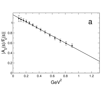
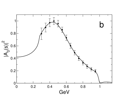
Figure 4: $J\psi\rightarrow\omega\pi\pi$ decay: energy dependence of the amplitude $|A_{0}(s)|$.

This demonstrates that the profile of the BES data on $|A_{0}(s)|$ closely resembles the one of the scalar form factor. In either case, there is a peak around $\sqrt{s}\simeq M_{\sigma}$, but the phase reaches $90^{\circ}$ only when the energy becomes about twice as large as the mass of the $\sigma$.

The low energy behaviour of the various amplitudes can be understood on the basis of twice subtracted dispersion relations. In the case of $\pi\pi$ scattering, the subtraction constants are predicted by chiral symmetry. As a consequence, the low energy behaviour of the phase shift $\delta^{0}_{0}(s)$ and the position of the pole from the $\sigma$ are understood. The symmetry, in particular, requires the occurrence of an Adler zero, which suppresses the scattering amplitude at low energies, so that the peak in that amplitude is pushed up, to $\sqrt{s}\simeq 2\,M_{\sigma}$. There is no such suppression in the decay amplitude, nor is there a prediction in that case: the two subtraction constants in the dispersion relation for $R(s)=A_{0}(s)/F_{0}(s)$,

$$R(s)=R_{0}+R_{1}\,s+\frac{(s-2M_{K}^{2})^{2}}{\pi}\!\int\!\frac{dx\,\mbox{Im}R(x)}{(x-2M_{K}^{2})\rule{0.0pt}{6.00006pt}^{2}\,(x-s)}\;\;,$$ (5)

must be taken from experiment. The integral receives a contribution from $s>4M_{K}^{2}$, as well as one from $s<0$. For definiteness, I have identified the subtraction point with the center of the interval between these two cuts. The straight line shown in Fig.4a is obtained by setting $s_{0}\equiv-R_{0}/R_{1}=1.65\,\mbox{GeV}^{2}$ and simply dropping the dispersion integral. Fig.4b shows that the approximation $A_{0}(s)\simeq R_{1}(s-s_{0})F_{0}(s)$ indeed accounts for the pronounced energy dependence seen in the BES data.

Above the range covered by the data points, the dispersive contributions presumably become quite important. In particular, the behaviour near the $K\bar{K}$ threshold need not be the same as the one of the non-strange form factor $F_{0}(s)$. As can be seen in Fig.4a, this form factor has a narrow dip there. The form factor of the operator $\,\overline{\rule[4.19998pt]{3.99994pt}{0.0pt}}ss$ instead exhibits a narrow peak ACCGL . If all final states other than $\pi\pi$ and $K\bar{K}$ are ignored, the general solution of the unitarity conditions is a linear combination of the two. An experimental investigation of the structure of $A_{0}(s)$ in the region of the $f_{0}(980)$ could shed some light on the importance of strange quarks in this context. At any rate, the zero, which a linear approximation for the ratio $R(s)$ necessarily entails, sits far beyond the region where that approximation is meaningful.

I do not see any reason to doubt that the BES data and the partial wave analysis thereof are correct. These clearly reveal the presence of the $\sigma$, but the pole positions extracted from simple Breit-Wigner treatments BES sigma of the amplitude $A_{0}(s)$ or more elaborate models Bugg sigma pole are subject to large theoretical uncertainties: the extrapolation off the real axis is sensitive to details of the parametrization that are not understood. In the language of dispersion theory, the problems arise from (a) the inelastic channels $\pi\pi\rightarrow K\bar{K}$ and $\pi\pi\rightarrow\eta\eta$, (b) the $f_{0}(980)$, (c) the left hand cut and (d) rescattering on the $\omega$. Unitarity and crossing symmetry very strongly constrain the scattering amplitude, but barely tell us anything about the transition $J/\psi\rightarrow\omega\pi\pi$.

We have applied our method to the models for the scattering amplitude proposed by Bugg Bugg sigma pole . The outcome for the mass and width of the $\sigma$ is close to the central values in Eq. (3). I conclude that our pole position is consistent with the BES data. There is a conflict only with the values for the mass and width obtained from the extrapolation of those models to complex values of $s$. It arises because the quoted errors do not account for the uncertainties inherent in such extrapolations Pennington .

References

- (1) I. Caprini, G. Colangelo and H. Leutwyler, Phys. Rev. Lett. 96 (2006) 132001.
- (2) S. Pislak et al. [BNL-E865 Collaboration], Phys. Rev. Lett. 87 (2001) 221801; Phys. Rev. D 67 (2003) 072004.
- (3) B. Adeva et al. [DIRAC Collaboration], Phys. Lett. B 619 (2005) 50.
- (4) J. R. Batley et al. [NA48/2 Collaboration], Phys. Lett. B 633, 173 (2006).
- (5) S. M. Roy, Phys. Lett. B 36 (1971) 353.
- (6) For a review, see D. Morgan and M. R. Pennington, in The Second DANE Physics Handbook, eds. L. Maiani, G. Pancheri and N. Paver, Frascati (1995), p. 193.
- (7) S. Weinberg, Phys. Rev. Lett. 17 (1966) 616.
- (8) J. Gasser and H. Leutwyler, Phys. Lett. B 125 (1983) 325; Annals Phys. 158 (1984) 142.
- (9) J. Bijnens, G. Colangelo, G. Ecker, J. Gasser and M. E. Sainio, Phys. Lett. B 374 (1996) 210; Nucl. Phys. B 508 (1997) 263; ibid. B 517 (1998) 639 (E).
- (10) G. Colangelo, J. Gasser and H. Leutwyler, Nucl. Phys. B 603 (2001) 125.
- (11) C. Aubin et al., [MILC Collaboration], Phys. Rev. D 70 (2004) 114501.
- (12) S. R. Beane, P. F. Bedaque, K. Orginos and M. J. Savage [NPLQCD Collaboration], Phys. Rev. D 73 (2006) 054503.
-
(13)
For recent reviews, see for instance
P. Minkowski and W. Ochs, AIP Conf. Proc. 814 (2006) 52; D. V. Bugg, AIP Conf. Proc. 814 (2006) 78; M. R. Pennington, Int. J. Mod. Phys. A 21 (2006) 747. - (14) N. A. Tornqvist and M. Roos, Phys. Rev. Lett. 76, 1575 (1996).
- (15) W.-M. Yao et al. [Particle Data Group], Journal of Physics G 33 (2006) 1.
- (16) A. Martin, Scattering Theory: Unitarity, Analyticity and Crossing, Lecture Notes in Physics, Vol. 3, (Springer-Verlag, Berlin, 1969).
- (17) S. M. Roy and G. Wanders, Nucl. Phys. B 141 (1978) 220.
- (18) The analysis of Zhou et al. Zhou is a notable exception. These authors use the two loop representation of PT to estimate the left hand discontinuity. The result is in good agreement with our analysis.
- (19) Z. Y. Zhou, G. Y. Qin, P. Zhang, Z. G. Xiao, H. Q. Zheng and N. Wu, JHEP 0502 (2005) 043.
- (20) B. Ananthanarayan et al., Phys. Rept. 353 (2001) 207.
- (21) V. E. Markushin and M. P. Locher, Frascati Physics Series, 15 (1999) 229.
- (22) R. L. Jaffe, Phys. Rev. D 15 (1977) 267, 281.
- (23) S. Descotes-Genon and B. Moussallam, hep-ph/0607133.
- (24) M. Ablikim et al. [BES Collaboration], Phys. Lett. B 598 (2004) 149.
- (25) D. V. Bugg, hep-ph/0608081.
- (26) I. Caprini, Phys. Lett. B 638 (2006) 468.
- (27) I thank D. Bugg for providing me with his numerical results for .
- (28) For a recent analysis, see B. Ananthanarayan et al., Phys. Lett. B602, 218 (2004).
- (29) The model for of Lähde and Meißner Lahde and Meissner corresponds to The form factor is taken from a unitarized version of PT . It is interesting to note that, in the version proposed by Hannah Hannah , the unitarized form factor contains a second sheet pole at MeV.
- (30) T. A. Lähde and U. G. Meißner, hep-ph/0606133.
- (31) T. Hannah, Phys. Rev. D 60 (1999) 017502.
- (32) M. R. Pennington, hep-ph/0608016, reaches essentially the same conclusion.