Classical and Non-Classical ADD-phenomenology with high-$E_{\perp}$ jet observables at collider experiments

Abstract:

We use the results from a recent investigation of hard parton–parton gravitational scattering in the ADD scenario to make semi-quantitative predictions for a few standard high-$E_{\perp}$ jet observables at the LHC. By implementing these gravitational scattering results in the P YTHIA event generator and combining it with the C HARYBDIS generator for black holes, we investigate the effects of large extra dimensions and find that, depending on the width of the brane, the relative importance of gravitational scattering and black hole production may change significantly. For the cases where gravitational scatterings are important we discuss how to distinguish gravitational scattering from standard QCD partonic scatterings. In particular we point out that the universal colorlessness of elastic gravitational scattering implies fewer particles between the hard jets, and that this can be used in order to distinguish an increased jet activity induced by gravitational scattering from an increased jet activity induced by eg. super-symmetric extensions where the interaction is colorful.

1 Introduction

The most exotic, and by far most discussed collider signal of large extra dimensions in the ADD scenario [1, 2, 3] is the copiously produced extra dimensional black holes [4, 5, 6, 7]. While these are expected to come with large cross sections and characteristic signals at the LHC for a “natural” Planck scale of around 1 TeV, both cross section and signals suffer severely from uncertainties associated with quantum gravity. This provides a wonderful chance to probe quantum gravity, but from the point of view of verifying the scenario it is not ideal. It is therfore worth looking for processes which involve fewer uncertainties than decaying black holes.

Other important ADD processes involve Kaluza–Klein modes, either the production of real ones, or the exchange of virtual ones in gravitational scattering of hard partons. The signal for the former involves a large missing transverse momentum and will be difficult to distinguish from eg. the production of stable super-symmetric particles in some SUSY extensions of the standard model. The later will show up as an increase of the jet cross sections at high energies and may, if this increase is is small, be difficult to distinguish from other beyond-the-standard-model effects.

In a previous paper [8] we investigated an alternative signal for the ADD scenario, namely the disappearance of the high-$E_{\perp}$ jet cross section due to the formation of black holes. However, in that paper we neglected the contribution from hard gravitational scattering.

Lately a coherent picture of gravitational scattering in the ADD model, at both low and high energies, was presented in [9]. In this paper we investigate the phenomenological consequences. Again, we will concentrate on standard jet observables to see how they are affected by the existence of large extra dimensions, using different choices of the model parameters. We will try to give a complete semi-quantitative description of the observables ranging from the region of perturbative gravitational scattering in the low-energy end to the domain of classical (non-quantum gravitational) black holes for energies above the Planck scale.

While the LHC should easily discover large extra dimensions for the most natural choices of Planck masses and number of extra dimensions, we find situations where no black holes are formed and the only gravitational scattering signal could be a slight increase of the $E_{\perp}$ and di-jet cross section at high energies. We therefore discuss the possibility of distinguish such scatterings from standard QCD events by studying the different color topologies involved. We also suggest that such a procedure could be used at the Tevatron to see if an increase of the high-$E_{\perp}$ jet cross section there could be the result of the onset of subplanckian gravitational scattering.

This paper is organized as follows. After a brief introduction to the ADD scenario in section 2, we summarize in section 3 the description of gravitational scatterings developed in [9]. We then go on to discuss the production and decay of black holes in section 4 and, in section 5, we present our results before discussing our conclusions in section 6.

2 Basics of ADD

The so called ADD scenario, invented in 1998 by Arkani-Hamed, Dvali and Dimopoulos [1, 2], aims at explaining the hierarchy problem, i.e. why the observed Planck scale at $10^{19}$ GeV is so large compared to the masses of the standard model particles. This is done by introducing a number, $n$, of extra dimensions in which only gravity is allowed to propagate.

In order to explain why these dimensions have not yet been observed, it is assumed that they are compactified with some (common) compactification radius $R$ and that no gauge fields are allowed to propagate in the extra dimensions. Gravity, on the other hand is, and this renders the form of Newton’s law at distances, $r$, much smaller than the compactification radius

$$\frac{V(r)}{m_{1}m_{2}} = -\frac{S_{n}\Gamma(n)}{M_{\mathrm{P}}^{n+2}(2\pi)^{n}}\frac{1}{r^{n+1}}.$$ (1)

Here $M_{\mathrm{P}}$ is the fundamental Planck scale, $S_{n}=2\pi^{n/2}/\Gamma(n/2)$ is the surface of a unit sphere in $n$ dimensions and $\Gamma(n)$ is the Euler Gamma function. At distances large compared to the compactification radius we must recover the normal 3+1-dimensional form of Newton’s law.

$$\frac{V(r)}{m_{1}m_{2}} = -G_{N(4)}\frac{1}{r}.$$ (2)

Expressing Newton’s constant in terms of the observed (3+1)-dimensional Planck scale, $G_{N(4)}\sim 1/M_{\mathrm{P4}}^{2}$, then gives the relation $M_{\mathrm{P4}}^{2}\sim M_{\mathrm{P}}^{n+2}R^{n}$ between the fundamental Planck scale $M_{\mathrm{P}}$ and the observed 4-dimensional Planck scale, which explains how the fundamental Planck scale could be (almost) of the same order as the weak scale, but the observed effective Planck scale, $M_{\mathrm{P4}}$, many orders of magnitude larger.

However, this also implies that gravity should be very strong at small distances which opens up for the possibility of observing gravitational scattering and black holes at collider experiments.

3 Gravitational scattering in ADD scenario

Although the field theory of gravity is ultimately divergent also in more than 4 dimensions, an effective low-energy theory can be constructed by a perturbative treatment of the metric in the limit where the metric perturbation is small. A Lagrangian can be derived and Feynman diagrams can be constructed from it. This is done in [10, 11]. Since the extra dimensions are compactified, momentum occurs in each direction as multiples of some ground frequency, ie. as Kaluza–Klein modes.

In a gravitational event an outgoing Kaluza–Klein (KK) mode will have some (quantized) momentum in the extra dimensions, which enters in the (3+1)-dimensional Lagrangian as a mass term. But the KK modes can also occur as intermediate states in which case they have to be properly summed or, taking the continuum limit, integrated over. This gives rise to the integral

$$\sum_{\overline{m}_{\overline{l}}}{\frac{1}{-m_{\overline{l}}^{2}+k^{2}}}\approx S_{n}R^{n}\int{\frac{m^{n-1}}{-m^{2}+k^{2}}}dm.$$ (3)

Here $\overline{l}$ enumerates the allowed momenta, $m_{\overline{l}}$, in the extra dimensions, $m$ is the absolute value of $m_{\overline{l}}$, and $k^{2}$ is the momentum squared of the $3+1$-dimensional part of the propagator. Note that this sum over KK states does imply momentum non-conservation for momenta transverse to the brane where the standard-model fields live, but this is not a complete surprise since translational invariance is broken in the bulk by the presence of the brane.

3.1 Dealing with divergences

What is worrying though, is that the field theory seems to contain divergences already at the tree level. However, the divergences dissappear when imposing the requirement that the standard model particles live on a brane, either directly by assuming a narrow distribution of the standard model fields into the extra dimensions [12, 9], or by a introducing a “brane tension” [13, 14]. Both these methods gives physical effective cut-offs for the momentum (mass) of the KK modes. For example, a Gaussian extension $e^{-m^{2}/(2M_{s}^{2})}$ of the standard model field densities into the bulk gives an “effective propagator” [9]

$$D(k^{2})=R^{n}S_{n}\int\frac{dm\,m^{n-1}}{k^{2}-m^{2}}e^{-m^{2}/M_{s}^{2}}$$ (4)

for the exchange of KK modes with four-momentum exchange $k^{2}$. (This object, $D(k^{2})$, is here sloppily called a propagator, despite the fact that the multiplicative Lorentz structure is not taken into account.)

For momentum exchange small compared to $M_{s}$, the standard model momentum $k$ in the propagator is irrelevant (for most $m$ in the integral), such that s-, t-, and u-channels are equally efficient and the scattering is fairly isotropic.

For $\sqrt{k^{2}}\gg M_{s}$ on the other hand, the interaction is dominated by forward scattering via the t-channel, and an all-order eikonal calculation is necessary to ensure unitarity [15, 9, 16]. The stage is therefore set by three energy scales, the fundamental Planck mass, $M_{\mathrm{P}}$, the inverse brane width (brane tension), $M_{s}$, and the rest mass of the partonic scattering, $\sqrt{s}$, and the phenomenology depend on their relative magnitude. It is illuminating to fix one of these scales an study the different kinematical regions in the plan spanned by the other two. This is done in fig. 1 where the $(\sqrt{s},M_{s})$-plane is plotted for $M_{\mathrm{P}}$ fixed to 1 TeV.

Below we will successively describe the contribution from the t-, u-, and s-channels and the various regions in fig. 1.

Figure 1: The $(\sqrt{s},M_{s})$-plane for $n=4$ and $M_{\mathrm{P}}=1$. The straight line separating region 1 and 4 is $\sqrt{s}=M_{s}$ while straight line separating region 4 and 5 is the line where the real and imaginary parts in eq. (16) have equal magnitude. The power-like solid curve separating region 1 and 2 is $\sqrt{s_{c}}$ from eq. (12) as a function of $M_{s}$ and the line separating the regions 4 and 5 from region 3 is the line where $|A_{\rm{Born}}X|=1$, see eq. (16). In the regions 1 and 2 $\sqrt{s}$ is larger than $M_{s}$, and, at least for $\sqrt{s}\gg M_{s}$, the eikonal approximation is correct. In region 1 the eikonal is, depending on $b$, either large compared to 1 or given by eq. (10). In region 2 on the other hand the $b$-range where $|\chi|$ is small includes a region where it is described by eq. (11). In region 3 the correction corresponding to higher order loops is small, but in region 4 it is important and helps assuring unitarity. The dashed line indicates the minimal $\sqrt{s}$ (for a given $M_{s}$) at which the black hole radius eq. (21) is larger than the brane width. The plot visibly very similar for n=6.

3.2 t-channel

As argued in the above section, we expect t-channel contributions to dominate at energies high compared to $M_{s}$. Unitarity constraints does, however, imply that the Born approximation can not be valid for sufficiently high energies. In fact, as is argued in [15, 17], a completely new phenomenon occurs for scattering in more than $3$ spatial dimensions; namely the emergence of a length scale associated with the transition from the classical to the quantum domain.

Intuitively this can be understood by considering the ratios

$$\frac{\Delta\theta}{\theta}\mbox{ and }\frac{\Delta b}{b}$$ (5)

where $\theta$ is the scattering angle and $b$ the impact parameter in a scattering experiment. In the classical domain these ratios are both much smaller than $1$. Requiring the opposite, and approximating

$$\Delta\theta\sim\frac{\Delta q}{Mv}\sim\frac{\hbar}{Mv\Delta b}\mbox{ and }\theta\sim\frac{b}{Mv^{2}}\frac{dV(b)}{db}$$ (6)

for a non-relativistic particle with speed, $v$, mass, $M$, and transverse momentum, $\Delta q$, moving in a potential, $V$, one finds, for a Coulomb-like potential $V(b)=\alpha/b$, the condition $\alpha<\hbar v$. For coupling constants close to $1$, this basically implies that the relativistic and quantum mechanical regions coincide. For a more general potential of the form $V(b)=\alpha/b^{n+1}$, assuming $n$ to be positive (this is what Gausses law gives in 3+n spatial dimensions), the separation of the classical and quantum domain depends on the impact parameter, such that, the transition occurs at $b_{c}\sim[\alpha/\hbar v]^{(1/n)}$. For gravitational coupling with $\alpha=G_{4+n}MM$, this corresponds to $b_{c}\sim[G_{4+n}M^{2}/(v\hbar)]^{1/n}$ [15]. Scattering in the potential eq. (1) is therefore expected to be mainly classical only if the impact parameter $b$ is smaller than $b_{c}$.

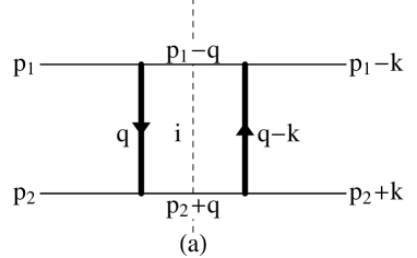
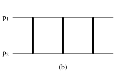
Figure 2: (a) The one loop contribution corresponding to exchange of two KK modes. The KK modes are drawn as thick lines and standard model particles as thin lines. (b) The two-loop contribution.

For $M_{\mathrm{P}}\sim 1$ TeV the parameters of this equation are such that we will see a transition between the classical and quantum domain at LHC, and a more careful calculation, summing up amplitudes from ladders of t-channel exchange in fig. 2 to all orders is necessary. This calculation was performed in [15] by simply ignoring the divergences corresponding to local contributions in eq. (3), and recently in [9] by a more careful analysis using the effective propagator eq. (4).

The parameter $b_{c}$ also corresponds to the impact parameter where the eikonal scattering phase

$$\chi(b) = \frac{1}{2s}\int\frac{d^{2}\bar{k}_{\perp}}{(2\pi)^{2}}\,e^{-i\bar{k}_{\perp}\bar{b}_{\perp}}A_{\rm{Born}}(-\bar{k}_{\perp}^{2})$$ (7)

becomes large compared to $\hbar$. This makes perfect sense, as $b_{c}$ represents the impact parameter separating quantum mechanical and classical scattering.

At least in the eikonal region, i.e. for small scattering angles, where there is no spin dependence, the Born amplitude can be written [9]

$$A_{\rm{Born}}(k^{2}=t)=\frac{s^{2}}{2^{n-3}\pi^{n-1}M_{\mathrm{P}}^{n+2}}\,S_{n}\int_{0}^{\infty}\frac{dm\,m^{n-1}}{k^{2}-m^{2}}\,e^{-m^{2}/M_{s}^{2}}$$ (8)

where the suppression factor $e^{-m^{2}/M_{s}^{2}}$ comes from implementing the requirement that the standard model particles live on a finite brane [9]. The same effect can be obtained by assuming a finite brane tension [13]. Computing the integrals in eq. (7) [9] then gives the result

$$\chi(b)=-\frac{sM_{s}^{n}}{(2\sqrt{\pi})^{n}M_{\mathrm{P}}^{n+2}}\Gamma(\frac{n}{2})U(\frac{n}{2},1,\frac{M_{s}^{2}b^{2}}{4})$$ (9)

where the $U$-functions are confluent hyper-geometric functions of the second kind.

In the limit of large third argument, $M_{s}b\gg 1$ in $U$, ie. impact parameters much larger than the brane width, $\chi$ can be written

$$\chi(b)\approx-\left(\frac{b_{c}}{b}\right)^{n}\,\,\,\,\mbox{for}\,\,\,\,b_{c} \equiv \frac{1}{\sqrt{\pi}}\left[\frac{s\Gamma(n/2)}{M_{\mathrm{P}}^{n+2}}\right]^{1/n}.$$ (10)

At least if $b_{c}\gg 1/M_{s}$ the eikonal eq. (9) reaches 1 in the region where it is determined by eq. (10) and $b_{c}$ is indeed the parameter associated with the transition from the quantum mechanical to the classical region. For $M_{s}$ small compared to $M_{\mathrm{P}}$ the brane width is more important and there is an energy range where the impact parameter for which $|\chi|$ reaches 1, is given by the small argument limit in $U$, rather than the large argument limit,

$$\chi(b) \approx \frac{2s}{(2\sqrt{\pi})^{n}M_{\mathrm{P}}^{2}}\left(\frac{M_{s}}{M_{\mathrm{P}}}\right)^{n}\left(\ln(M_{s}b)+\frac{1}{2}\psi(\frac{n}{2})\right)$$ (11)

where $\psi(\frac{n}{2})$ is the digamma function. The transition between, $|\chi(b)|\approx 1$ described by eq. (11), and $|\chi(b)|\approx 1$ described by eq. (10), occurs roughly at the energy where $b_{c}=1/M_{s}$, and the phenomenology will therefore differ in the regions $b_{c}>1/M_{s}$ and $b_{c}<1/M_{s}$. Solving $b_{c}=1/M_{s}$ we find

$$s_{c}=\frac{M_{\mathrm{P}}^{n+2}\pi^{n/2}}{M_{s}^{n}\Gamma(\frac{n}{2})}$$ (12)

this is the line separating region 1 and 2 in fig. 1. For $t\gg M_{s}^{2}$ the all order eikonal amplitude is given by

$$A_{\rm{eik}}(k^{2})=-2is\int d^{2}\bar{b}_{\perp}e^{i\bar{k}_{\perp}\cdot\bar{b}_{\perp}}(e^{i\chi}-1).$$ (13)

When $|\chi|$ is large compared to 1 which, for $b_{c}\gg 1/M_{s}$, happens for $b<b_{c}$, the exponentiation in eq. (13) is important while for larger $b$ the eikonal amplitude is approximated by the Born term.

For $b_{c}<1/M_{s}$, region 2 in fig. 1, $|\chi|$ is smaller than 1 except for very small impact parameters,

$$b<\frac{1}{M_{s}}\exp\left(-\frac{(2\sqrt{\pi})^{n}M_{\mathrm{P}}^{n+2}}{2sM_{s}^{n}}\right),$$ (14)

found by ignoring the digamma function in eq. (11). In the whole of region 1 and 2 for $t\gg M_{s}^{2}$ the gravitational cross section is obtained from the all order eikonal amplitude in eq. (13) (although higher order corrections are only important region 1). It is given by

$$\frac{d\sigma_{\rm{eik}}}{dt}=\frac{1}{16\pi s^{2}}|A_{\rm{eik}}|^{2}.$$ (15)

If, on the other hand, $\sqrt{s}\ll M_{s}$, such that $\sqrt{-t}$ necessarily is small compared to $M_{s}$, the Born amplitude is (apart from large angle spin dependences) fairly isotropic. The ladder-type diagrams in fig. 2 will effectively turn into $\phi^{4}$ interactions as in fig. 3.

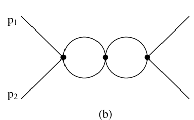
Figure 3: When the exchanged momentum is small compared to $M_{s}$, the KK propagator are effectively replaced by vertex factors. The diagrams in fig. 2 can then be drawn as above with only standard model particle lines.

Since the coupling grows with energy, higher order corrections will for some $s$ become necessary to ensure unitarity. Summing up all contributions of the type in fig. 3, neglecting large angle spin dependence, a geometric series is found [9] which helps unitarizing the cross section. For the 1-loop contribution we have, with $P=p_{1}+p_{2}$ as in fig. 3,

$$A_{\rm{1-loop}} \approx \frac{-i}{2}\int_{q<M_{s}}\frac{d^{4}q}{(2\pi)^{4}}A_{\rm{Born}}^{2}\frac{1}{(P/2-q)^{2}}\frac{1}{(P/2+q)^{2}}=$$ (16)

$$\equiv A_{\rm{Born}}^{2}\cdot X\,\,\mathrm{with}\,\,X\approx\frac{1}{32\pi^{2}}(\ln\frac{M_{s}^{2}}{s/4}+i\pi)$$

and higher loop corrections give similar results. Summing all ladders we obtain

$$A_{\mathrm{ladders}}=A_{\rm{Born}}\,(1+A_{\rm{Born}}X+(A_{\rm{Born}}X)^{2}+\ldots\ )=\frac{A_{\rm{Born}}}{1-A_{\rm{Born}}X}.$$ (17)

Thus loop contributions of this type helps unitarizing the cross section in region 4 in fig. 1, defined to be the region where $\sqrt{s}<M_{s}$, but on-shell intermediate states in fig. 3 dominate. While we can not prove that these are the most important contributions, it seems likely as long as the cross section is dominated by on-shell states. In region 5 in fig. 1 this is no longer true since here the imaginary part in eq. (16) is smaller than the real part. The simulations performed in this paper are in the phase space region 1, 2, 3 and 4 in fig. 1, and we use eq. (16) to unitarize the cross section in regions 3 and 4 (although it’s not important in region 3).

3.3 u-channel

In the regions 1 and 2, the u-channel contribution (here generally defined to be the case where the outgoing particle lines are crossed compared to the incoming) is small compared to forward t-channel scattering. In the regions 3 and 4, corresponding to $\sqrt{s}<M_{s}$, it is, however, of the same order of magnitude. In fact there is no difference between the u and t-channel in fig. 3. This implies that u-channel contributions run into problems with unitarity at roughly the same energy as t-channel contributions, and the result eq. (17) (again neglecting spin dependence) can be used also for the u-type ladders.

The relevance of the u-channel ladders contribution is, however, significantly lowered by the fact that interaction among identical partons is suppressed at LHC. To get a handle on the importance of u-channel contribution, assume that only valence quarks contribute to the cross section. This is a reasonable assumption at sufficiently high momentum fractions and also, it will give an upper limit. The probability for the colliding partons to have identical flavor, spin and color is then approximately $1/10$.

3.4 s-channel

For $s\ll M_{s}^{2}$, the factor $k^{2}=s$ in eq. (8) is insignificant compared to most contributing KK masses and gives an amplitude similar to the t- and u-channels. There is, however, one complication. Due to the relative difference in sign between $k^{2}=s$ and $m^{2}$ in eq. (8) KK modes can be produced on shell.

From the point of view of inclusive observables, these s-channel on-shell Kaluza–Klein states are, however, unimportant. The width of a single KK mode with mass $m$ to decay into two standard model particles of energy $m/2$ is $\sim m^{3}G_{N(4)}$ giving lifetimes of order 1000 seconds [11]. These KK modes will leave the detectors unseen.

3.5 Phenomenology of low energy gravitational scattering

As already mentioned section 3.1, a gravitational scattering where the Kaluza-Klein mode is not in the outgoing state, comes with a momentum cut-off from the width of the brane, or from fluctuations of the brane. In the low-energy region, 3 in fig. 1, where the born approximation is applicable, a cut-off dependent amplitude can be used for describing the interaction. From the point of view of perturbative gravitational scattering with internal KK modes only, this does not result in any extra parameters to describe the interaction. Instead it suffice to replace the Planck scale $M_{\mathrm{P}}$ by an effective Planck scale according to

$$M_{\mathrm{eff}}=\frac{1}{2}\left(\frac{(n-2)2^{n}\pi^{\frac{n-2}{2}}M_{\mathrm{P}}^{n+2}}{M_{s}^{n-2}}\right)^{\frac{1}{4}}$$ (18)

such that the Born amplitude, eq. (8), (neglecting spins) can be written

$$A_{\rm{Born}}=-\frac{s^{2}}{M_{\mathrm{eff}}^{4}},$$ (19)

after integration over $m$, neglecting $k^{2}=t$, $u$ or $s$. In this kinematical region, gravitational scattering in the ADD model is a well behaved effective field theory depending on only one free parameter, $M_{\mathrm{eff}}$. The low-energy spin dependent footprint of the ADD scenario for any number of extra dimensions can then be written

$$\frac{d\sigma}{dt}=\frac{k_{s}}{s}\left[\frac{\pi\alpha_{s}^{2}}{s}f(z)-\frac{s\alpha_{s}}{M_{\mathrm{eff}}^{4}}g(z)+\frac{s^{3}}{\pi M_{\mathrm{eff}}^{8}}h(z)\right]$$ (20)

where $\alpha_{s}$ is the strong coupling constant and $k_{s}$, $g(z)$, $h(z)$ and $f(z)$ are process dependent functions taking spin-dependence into account given in [18].

Gravitational scattering differ from standard-model and most beyond-standard-model processes in several ways. The experimentally most striking is probably that it increases with increasing energy. As the experimental situation stands today this is, however, badly overcompensated by the decreasing parton distribution functions for high momentum factions. The interaction is mediated by the large number of Kaluza–Klein modes, implying that the cross section will not have a single resonance structure, as opposed to cross section signatures of most other beyond-standard-model particles. Due to the different spin dependence of gravitational scattering the angular distribution will also differ.

We will here consider another difference, namely that contrary to the main contribution to inclusive cross sections, both in the standard model and in super-symmetric extensions, the gravitational interaction is colorless. As we shall see, this implies noticeable differences in particle multiplicity outside the jets.

4 Black holes in ADD scenario

Black holes with mass large compared to the fundamental Planck scale, but with radius small compared to the compactification radius are expected to behave much like extra dimensional versions of astronomical 3+1-dimensional black holes. The Schwarzschild radius is given by

$$r_{\mathrm{Sch}}=\frac{1}{\sqrt{\pi}M_{\mathrm{P}}}\left[\frac{M_{\mathrm{BH}}}{M_{\mathrm{P}}}\frac{8\Gamma(\frac{n+3}{2})}{n+2}\right]^{\frac{1}{n+1}}$$ (21)

and the temperature is given by [19]

$$T=\frac{n+1}{4\pi r_{\mathrm{Sch}}}.$$ (22)

Note that small black holes are hotter.

A major difference between black holes in the ADD scenario and ordinary 3-dimensional black holes is that ADD black holes do not radiate gauge fields into most of phase space, since only gravity is allowed to propagate in the extra dimensions. One may believe that this would lead to almost no radiation on the brane (where gauge fields and, hence, also we live) as the bulk phase space is much larger. However, it has been shown that this is not necessarily the case [4].

Since we are considering the non-idealized situation of a finite brane width we must also consider the implications of this on black hole production. In particular, a natural requirement is that the brane is not more extended than the black hole, leading to the condition $r_{\mathrm{Sch}}<1/M_{b}$ for the formation of black holes. As we will see this prevents black holes from appearing at the LHC for sufficiently small $M_{s}$.

On the other hand, if $M_{s}$ is large, we may, with increasing $\sqrt{s}$, go directly from the Born region 3 in fig. 1 to black hole production. This should be worrying since the black holes are treated semi-classically but the gravitational scattering in region 3 is purely quantum mechanical. It is reasonable that the black holes should start behaving classically when the Compton wave length is of the same order as the black hole radius, but it would have been more comforting to only study black hole production in region 1 in fig. 1, where the gravitational scattering is mainly classical already at lower energies. This represents a genuine quantum gravity uncertainty.

Already at a classical level the cross section for black hole creation is subject to significant uncertainties. This is basically due the fact that it does not suffice to consider the colliding objects, but in addition the curvature of space-time far outside the black hole need to be calculated. Classical numerical simulations for black hole formation in extra dimensions have been performed in [20, 21] with the result that the geometric cross section, $\pi r^{2}$, should be multiplied with a factor $\sim 0.7-3$, increasing with the number of extra dimensions. For this paper we have, however, chosen to keep the constant at 1.

As the black holes considered here are formed from partons inside the protons there is also an uncertainty from the usage of parton distribution functions for an essentially non-perturbative process [22] . (A discussion about the effects of quantum fluctuations based on wave packages can be found in [23, 24].)

Then there is the question of the onset of black hole production. It can be argued that no black holes should be formed below (roughly) the Planck scale as the uncertainty principle would forbid sufficient localization of the partons. But precisely when does black holes begin to form?

We consider first the condition that the black holes have to be well localized in our ordinary dimension. Looking at the momenta of the incoming partons in their combined rest frame it is reasonable to require that their wavelength, $\lambda_{l}\propto 2/\sqrt{s}$, is less than $r_{\mathrm{Sch}}$. The corresponding requirement in the transverse direction gives the requirement: $\lambda_{\perp}\propto 1/p_{T}<r_{\mathrm{Sch}}$. Clearly one can argue about the proportionality constant. We have chosen

$$M_{\mathrm{min}}=2/r_{\mathrm{Sch}}(M_{\mathrm{min}}).$$ (23)

Combining this with the expression for the Schwarzschild radius eq. (21) we get

$$M_{\mathrm{min}}={M_{\mathrm{P}}}\left[\frac{(2\sqrt{\pi})^{n+1}(n+2)}{8\Gamma(\frac{n+3}{2})}\right]^{\frac{1}{n+2}}.$$ (24)

Numerically the value of $M_{\mathrm{min}}$ is then approximately twice the Planck mass.

As we consider a finite brane width we must add the condition $r_{\mathrm{Sch}}>1/M_{s}$, leading to the minimal mass

$$M_{\mathrm{min2}}=\frac{M_{\mathrm{P}}^{n+2}(2+n)\pi^{\frac{n+1}{2}}}{8\Gamma\left[\frac{3+n}{2}\right]M_{s}^{1+n}}.$$ (25)

Again one can argue about the proportionality constant. While we take into account the effects of a finite brane, we do not consider the dynamics governing the brane, and possibly describing its width, although this may have significant effects on the spectra observed [25, 26].

Once a black hole has formed it is believed to lose most of its geometric asymmetries in a short period referred to as the balding phase. This phase leaves a black hole whose only geometric asymmetry can be described by one angular momentum parameter. However, it turns out that this angular momentum tends to be lost rather quickly via Hawking radiation, such that the black hole (apart from gauge charges) can be described by the Schwarzschild metric.

Neglecting the gauge charges, which in the case of electromagnetism has been shown to have a modest influence [27], the disappearance of the black hole would be well described by Hawking radiation if the black hole was much heavier than the Planck mass, and if no brane effects, such as the black hole recoiling of the brane [28, 29], or interacting with the brane [25, 26] is taken into account. The problem is that most collider-produced black holes will not be much heavier than the Planck mass.

For a hole which is not heavy compared to the Planck mass one cannot treat the metric as a static background for the emitted quanta, the back-reaction of the quanta to the metric should be taken into account and this is not done in the derivation of the Hawking radiation [30]. Also, at some point, the lifetime of the black hole becomes shorter than its radius. This makes it difficult to talk about a thermalized black hole.

Considering all of this, it should not come as a surprise if black holes where observed with spectra which differs significantly from that expected from eq. (22).

5 Results

We have used the amplitudes for gravitational scattering for the different regions in fig. 1 presented above to reweight the standard QCD $2\to 2$ scatterings in the P YTHIA (version 6.2 [31]) event generator. In the regions 1 and 2 we have used the (elastic spin-independent t-type) all order eikonal cross section from eq. (7) and eq. (13). In the regions 3 and 4 we have used the spin dependent Born amplitude [32] corresponding to eq. (20), and higher order corrections according to eq. (17). In region 3 the higher order corrections are small, but in region 4 they are essential. In the case of particle-antiparticle scattering, such that the scattering can be mediated via the s-channel, we have “unitarized” also the s-channel contribution in region 4 (and 3) using eq. (17), despite that fact the the s-type ladders, diagrams in fig. 3 rotated by $\pi/2$ do not have on-shell intermediate standard model particles. There are thus several fundamental uncertainties associated with gravitational scattering in region 4. First, we use the spin dependent Born amplitude, but we do not take spin dependence consistently into account in eq. (17) since we use the same $A_{\rm{Born}}(t)$ everywhere in all ladders. Second, we suppress s-type contributions in the same way as u- and t-type. (Note that we call the ladders in fig. 2 and fig. 3 t-type, sometimes these diagrams are referred to as s-channel, since the resummation is in $s$.)

The different treatments in the various regions means that we could expect a discontinuous transition when $\sqrt{s}$ is increased, such that we cross the line $\sqrt{s}=M_{s}$ in fig. 1. As long as the Born approximation is applicable (regions 2 and 3), this transition just corresponds to starting neglecting spin-dependence in region 2. If the transition is between region 4 and 1, the situation is, however, worse due to fundamental uncertainties associated with region 4.

For each generated $2\to 2$ scattering we also change the color flow between the scattered partons with a probability $\sigma_{\mathrm{ADD}}/(\sigma_{\mathrm{ADD}}+\sigma_{\mathrm{QCD}})$ to reflect the colorless nature of the graviton exchange. The resulting partonic state is then allowed to evolve a QCD cascade and is finally hadronized to produce fully simulated hadron-level events. Where relevant, we have also added multiple soft and semi-hard QCD scatterings to simulate the underlying event according to the model implemented in P YTHIA [33].

In addition, we have used the C HARYBDIS [34] program to simulate the production and decay of black holes as described in section 4 and in [8]. To ensure that the energy is sufficiently localized, in our ordinary dimensions and in the extra dimensions, we have required a minimal black hole mass according to eq. (24) and eq. (25). We also use the Schwarzschild radius to cut off any QCD and gravitational $2\to 2$ scatterings in region 3 and 4 for large enough masses and transverse momenta as discussed in [8]. In region 1 (and 2) we use the impact parameter description defined via eq. (9) to turn off gravitational interactions at distances smaller than $r_{\mathrm{Sch}}$. Clearly this simpleminded approach of turning of gravitational scattering should not be seen as the final word. In particular our understanding of gravitational scattering, and hence its turnoff, is limited in region 4.

We limit our investigation to two standard inclusive high-$E_{\perp}$ jet observables [8, 22, 35], namely the $E_{\perp}$-spectrum of the highest-$E_{\perp}$ jet in an event, and the distribution in invariant mass, $M_{jj}$, of the two highest-$E_{\perp}$ jets in an event. As high-$E_{\perp}$ jets will be a part of almost any signal of new physics at the LHC, such observables will be measured early on after the start of the experiments and it is also where one would expect gravitational scatterings to contribute. We use a simple cone algorithm with a code radius of 0.7, assuming a calorimeter covering the pseudo-rapidity interval, $|\eta|<2.5$, and requiring a minimum $E_{\perp}$ of $100$ GeV for the resulting jets. We have checked that our results do not depend much on the algorithm chosen.

$M_{\mathrm{eff}}$	$n$	$M_{s}/M_{\mathrm{P}}$	$M_{\mathrm{P}}$	$M_{s}$
1.0	4	$\frac{1}{2}$	0.45	0.22
1.0	4	1	0.63	0.63
1.0	4	2	0.89	1.79
1.0	4	4	1.26	5.05
1.0	6	2	0.56	1.13
0.7	4	4	0.88	3.54
4.0	4	4	5.05	20.21

Table 1: The different values of $M_{\mathrm{eff}}$, number of extra dimensions, $n$, and the ratio of $M_{s}/M_{\mathrm{P}}$ used in the simulations together with the resulting approximative values of $M_{\mathrm{P}}$ and $M_{s}$. The masses are all given in units of TeV.

Figure 4: (a) The $E_{\perp}$-spectrum of the highest $E_{\perp}$ jet in an event, and (b) the invariant mass spectrum of the two highest $E_{\perp}$ jets in an event at the LHC. In both cases $M_{\mathrm{eff}}=1$ TeV with 4 extra dimensions and $M_{s}/M_{\mathrm{P}}=2$ ($M_{\mathrm{P}}\approx 0.9$ TeV, $M_{s}\approx 1.8$ TeV). The long-dashed lines are the contribution from QCD scatterings, short-dashed lines the contribution from gravitational scatterings, dotted lines the contribution from the decay of black holes and full lines the sum of all contributions.

In fig. 4 we show generated the $E_{\perp\mathrm{max}}$ and $M_{jj}$ distributions at the LHC for the case of four extra dimensions, $M_{\mathrm{eff}}=1$ TeV and $M_{s}/M_{\mathrm{P}}=2$ (see table 1 for the resulting values of $M_{\mathrm{P}}$ and $M_{s}$). In the $E_{\perp\mathrm{max}}$ spectra we see that the cross section is dominated by QCD scatterings at low $E_{\perp}$as expected, followed by an intermediate region where gravitational scattering becomes important before black-hole production starts dominating the cross section at large $E_{\perp}$. For the $M_{jj}$-spectrum, the situation is different, and the gravitational scatterings dominates at large masses.

Modulo effects of the parton densities we expect both gravitational scattering and black-hole production to increase with energy. For black holes one may naively not necessarily expect to find high-$E_{\perp}$ jets, as energetic quanta are Boltzmann suppressed in the Hawking radiation. However, it turns out that the large cross section for a black hole to form at high $s$, multiplied with the small probability for the Black hole to radiate extremely energetic quanta, may dominate over the non-black hole cross section for rather large transverse momenta [8]. (Even if well localized QCD and gravitational scattering events are not suppressed due to black hole production.) These extremely energetic quanta do, however, not obey the semiclassical approximation in the Hawking radiation derivation, and are therefore associated with large uncertainties.

For large $E_{\perp}$, however, the gravitational scattering events, just as the QCD ones, may be localized inside the Schwarzschild radius and will collapse into a black hole.

Figure 5: The contribution of different regions in figure 1 to the di-jet mass spectrum from gravitational scatterings at the LHC with $M_{\mathrm{eff}}=1$ TeV, 4 extra dimensions and $M_{s}/M_{\mathrm{P}}=1$ (a), $2$ (b) and $4$ (c). In all cases the full line is the sum of all contributions and the contributions from regions 1, 2, 3 and 4 is given by the long-dashed, short-dashed, dotted and dash-dotted lines respectively.

In fig. 5 we show the $M_{jj}$-distribution of gravitational scatterings only, divided into the contributions from the different regions in fig. 1. Keeping $M_{\mathrm{eff}}=1$ TeV and the number of extra dimensions (4) fixed, we vary $M_{s}/M_{\mathrm{P}}$ and find that the contribution from region 1 dominates except in the low-mass regions below $M_{s}$. The transitions between the regions are not sharp, mainly due to the smearing introduced by shower, hadronization and the jet reconstruction. This smearing hides the fact that the transition between $\sqrt{s}>M_{s}$ and $\sqrt{s}<M_{s}$ is discontinuous in the distribution of the generated $s$. In the case this transition occurs between region 2 and 3, where the Born approximation is applicable, the discontinuity is not even visible in the generated $s$-distribution. If the transition occurs between region 4 and 1, a discontinuity can, however, be seen.

Figure 6: The same as fig. 4a, but with $M_{s}/M_{\mathrm{P}}=1$ (a), $4$ (b) and $0.5$ (c).

We note in table 1 that, although $M_{\mathrm{eff}}$ is kept fixed, giving the same amount of gravitational scattering at $\sqrt{s}\ll M_{s}$, increasing the ratio $M_{s}/M_{\mathrm{P}}$ will increase both $M_{s}$ and $M_{\mathrm{P}}$. And since black-hole production depends of $M_{\mathrm{P}}$ and $M_{s}$ differently via eqs. (21), (23) and (25), we can vary the relative importance of gravitational scattering and black-hole production by varying $M_{s}/M_{\mathrm{P}}$. Hence we see in fig. 6a that lowering $M_{s}/M_{\mathrm{P}}$ to 1, the gravitational scattering will never give a sizeable contribution to the $E_{\perp\mathrm{max}}$-distribution, while increasing the ratio to 4 (fig. 6b) results in the gravitational scattering dominating the cross section further out in $E_{\perp}$ as compared to fig. 4a. In fig. 6c we decrease the ratio even further to 0.5 which results in a brane thickness so large that black holes can never be formed at the LHC, and the only indication of the presence of extra dimensions in the $E_{\perp}$spectra is a slight increase in the cross section for large $E_{\perp\mathrm{max}}$.

Figure 7: The same as fig. 4a, but with (a) 4 extra dimensions, $M_{\mathrm{eff}}=4$ TeV, $M_{s}/M_{\mathrm{P}}=4$ and (b) 6 extra dimensions, $M_{\mathrm{eff}}=1$ TeV, $M_{s}/M_{\mathrm{P}}=2$.

A similar effect can be obtained by increasing the effective mass, while keeping the ratio $M_{s}/M_{p}$ fixed, hence increasing both $M_{\mathrm{P}}$ and $M_{s}$. This is done in fig. 7a and, again, the only visible effect of the extra dimensions is from gravitational scattering in the high-$E_{\perp}$ region. On the other hand we see in fig. 7b how increasing the number of extra dimensions to 6, keeping $M_{\mathrm{eff}}=1$ TeV, gives a negligible contribution from gravitational scattering to the $E_{\perp\mathrm{max}}$-distribution, which instead is completely dominated by the decay of black holes.

If large extra dimensions exist, one would hope that the scales are such that they would be easily discovered at the LHC by, eg. the striking signature of a decaying black hole. However, it is easy to see how nature could conspire, such that the only signal in the $E_{\perp}$ spectrum would be a slight increase of the high-$E_{\perp}$ jet cross section. There are, of course, other signals, such as the production of real gravitons, showing up as large missing transverse momenta. But such signals could also be the result of other possible beyond-the-standard-model scenarios. In any case, it would be desirable to be able to distinguish gravitational scatterings from standard QCD events. One obvious difference is that the exchange of a graviton is colorless in contrast to a QCD scattering. This will necessarily give rise to a different color topology in gravitational events as compared to QCD ones. In particular one would expect the appearance of so-called rapidity gaps between the jets in gravitational scattering events. Although these gaps may be filled by secondary soft and semi-hard QCD scatterings, one may still expect a lower activity between the jets in such events.

Figure 8: The average number of charged particles outside the jet-cones in the central rapidity unit between the two hardest jets in events corresponding to fig. 6c. The full line is for all events while the long-dashed and short-dashed are for QCD and gravitational scatterings respectively. In (b) only events with a minimum pseudo-rapidity difference of one unit between the two highest $E_{\perp}$ jets are included, while in (a) there is no such requirement.

In fig. 8a we show the average number of charged particles with a transverse momentum above $0.5$ GeV outside the jet cones in the middle unit of pseudo-rapidity between the two hardest jets as a function of $E_{\perp\mathrm{max}}$. Hence, we count only charged particles, $c$, with

$$p_{\perp c} > 0.5\mbox{~{}GeV},$$

$$\Delta R_{c1},\Delta R_{c2} > 0.7\mbox{~{}and}$$

$$\left|\eta_{c}-\frac{\eta_{1}+\eta_{2}}{2}\right| < 0.5,$$ (26)

where $\eta_{c}$ and $\eta_{i}$ are the pseudo rapidities of the particle and (the center of) jet $i$ respectively and $\Delta R_{ci}$ is the distance between the particle and jet $i$ in the pseudo-rapidity–azimuth-angle $(\eta,\phi)$ plane. In this simulation we have included multiple interactions in P YTHIA to simulate the underlying event. We see that the expectation from QCD events is around 10 particles, while for gravitational scatterings the average is around 5. With sufficient statistics it could therefore be possible to observe the decrease in the number of charge particles with increasing $E_{\perp\mathrm{max}}$ as gravitational scatterings starts to dominate. In fig. 8a we have not required a large rapidity separation between the jets. Doing so would increase the effect, as shown in fig. 8b, but on the other hand the statistics would decrease.

We note that the absolute numbers in fig. 8 is very sensitive to the modeling of the underlying event, which is very difficult to predict for the LHC. The underlying event should, however, give the same contribution to both scattering types, and the difference between the two should be fairly well predicted by P YTHIA .

Figure 9: (a) The $E_{\perp}$-spectrum of the highest $E_{\perp}$ jet in an event, and (b) The average number of charged particles outside the jet-cones in the central rapidity unit between the two hardest jets at the Tevatron for $M_{\mathrm{eff}}=700$ GeV, $M_{s}/M_{\mathrm{P}}=4$ and 4 extra dimensions. The full line is for all event while the long-dashed and short-dashed are for QCD and gravitational scatterings respectively.

At the Tevatron there was an indication of an excess of the cross section for very high $E_{\perp}$ jets as compared to the QCD prediction [37, 38]. Although a re-evaluation of the uncertainties due to the parton density parameterizations used in the QCD calculations has brought this excess within the limits of the statistical and systematical errors, it is still intriguing that such an excess could be the signal of the onset of gravitational scattering due to the presence of large extra dimensions.

In fig. 9a we show our prediction for the $E_{\perp\mathrm{max}}$ distribution for $n=4$, $M_{\mathrm{eff}}=700$ GeV and $M_{s}/M_{\mathrm{P}}=4$ at the Tevatron. The parameters were chosen so that the excess above standard QCD production is approximately within the statistical and systematical uncertainties of the corresponding Tevatron measurement. In fig. 9b we then show the average number of charged particles outside the cones (same as in fig. 8, but counting charged particles with transverse momenta down to $0.25$ GeV). The decrease in the region where gravitational scatterings become important is significant, although it may be difficult to get enough statistics to measure it even for Run-II at the Tevatron. However, it is not completely inconceivable that by finding a more sensitive observable of the color structure, we could be able to see the first indication of large extra dimensions already at the Tevatron, before LHC is switched on.

6 Conclusions

We have studied gravitational scattering and black hole production at the LHC and the Tevatron in the ADD scenario assuming that brane on which the standard model fields live have a finite width. We found that the relative importance of gravitational scattering and black hole production is sensitive to this width, and that for large widths the extension of the standard model particle fields into the bulk, may prevent black holes from forming since the energy may not be sufficiently localized within the black hole radius.

A wide brane corresponds to a low cut-off for virtual Kaluza–Klein modes (the brane width and the KK cut-off, $M_{s}$, are inversely related via a Fourier transform [9]) and therefore results in weaker gravitational interaction in the non-classical regions. It is thus possible for nature to conspire, by choosing a low $M_{s}$, such that neither much gravitational scattering or black holes is observed at the LHC. In this case processes involving the production of on-shell KK modes resulting in missing $E_{\perp}$ may become important observables.

In our simulations we have used values of $M_{\mathrm{P}}$, $M_{s}$ and the number of extra dimensions, $n$, which we believe have not yet been excluded by experiments (see eg. [39, 40] for recent reviews). Most of these limits are only relevant to $M_{\mathrm{P}}$  but restrictions on $M_{s}$ could be obtained by considering processes involving both virtual and real KK modes.

In the case of low $M_{s}$, only a weak increase in the jet spectra could be observed at LHC, and the signal of missing $E_{\perp}$ could be the result of SUSY. We point out that the colorless nature of gravitational scattering could be a way of distinguishing gravity induced events from other beyond-standard-model extensions. In fact this method could be used to indicate if an excess of jet activity at high transverse energies at the Tevatron is a result of gravitational scattering.

Appendix A Appendix

There are at least four definitions of the Planck mass. Often one have to understand which definition an author uses by the relation of the Planck mass to the 4-dimensional Newton’s constant $G_{N(4)}$ or to the Schwarzschild radius of a black hole. The process of hunting down constants is further complicated by the use of different definitions of the compactification radius, many authors [10] mean by the compactification radius rather the compactification circumference, here denoted $L$, whereas others really mean the radius, $R=L/(2\pi)$. In order to simplify comparison between the different conventions we here state the relations between the Planck masses $M_{\mathrm{P}}$ (used here) and in [34], $M_{D}$ used in [11, 15], $M_{G}$, $M_{S}$ used in [10] and the 4-dimensional Newton’s constant $G_{N(4)}$, the relation between the Planck masses and Schwarzschild radius, and the relations of the Planck masses to each other.

$$M_{D}^{2+n}=\frac{1}{8\pi R^{n}G_{N(4)}}$$ (27)

$$M_{\mathrm{P}}^{2+n}=\frac{1}{L^{n}G_{N(4)}}$$ (28)

$$M_{G}^{2+n}=\frac{2^{n-2}\pi^{n-1}}{L^{n}G_{N(4)}}$$ (29)

$$M_{S}^{2+n}=\frac{\Gamma\left(\frac{n}{2}\right)\pi^{n/2}}{2^{1-n}L^{n}G_{N(4)}}$$ (30)

$$r_{\mathrm{Sch}}=\frac{1}{M_{D}}\left[\frac{M_{BH}}{M_{D}}\right]^{\frac{1}{n+1}}\left[\frac{2^{n}\pi^{\frac{n-3}{2}}\Gamma\left(\frac{n+3}{2}\right)}{n+2}\right]^{\frac{1}{n+1}}$$ (31)

$$r_{\mathrm{Sch}}=\frac{1}{\sqrt{\pi}M_{\mathrm{P}}}\left[\frac{M_{BH}}{M_{\mathrm{P}}}\right]^{\frac{1}{n+1}}\left[\frac{8\Gamma\left(\frac{n+3}{2}\right)}{n+2}\right]^{\frac{1}{n+1}}$$ (32)

$$r_{\mathrm{Sch}}=\frac{2}{M_{G}}\left[\frac{M_{BH}}{M_{G}}\right]^{\frac{1}{n+1}}\left[\frac{\pi^{\frac{n-3}{2}}\Gamma\left(\frac{n+3}{2}\right)}{n+2}\right]^{\frac{1}{n+1}}$$ (33)

$$r_{\mathrm{Sch}}=\frac{1}{M_{S}}\left[\frac{M_{BH}}{M_{S}}\right]^{\frac{1}{n+1}}\left[\frac{2^{2+n}\Gamma\left(\frac{n+3}{2}\right)\Gamma\left(\frac{n}{2}\right)}{\sqrt{\pi}(n+2)}\right]^{\frac{1}{n+1}}$$ (34)

$$M_{\mathrm{P}} = 2^{\frac{3-n}{2+n}}\pi^{\frac{1-n}{2+n}}M_{D}$$ (35)

$$= 2^{\frac{2-n}{2+n}}\pi^{\frac{1-n}{2+n}}M_{G}$$

$$= 2^{\frac{1-n}{2+n}}\pi^{\frac{-n}{4+2n}}\Gamma\left(\frac{n}{2}\right)^{\frac{-1}{2+n}}M_{S}$$

References

- [1] N. Arkani-Hamed, S. Dimopoulos, and G. R. Dvali Phys. Lett. B429 (1998) 263–272, hep-ph/9803315.
- [2] N. Arkani-Hamed, S. Dimopoulos, and G. R. Dvali Phys. Rev. D59 (1999) 086004, hep-ph/9807344.
- [3] I. Antoniadis, N. Arkani-Hamed, S. Dimopoulos, and G. R. Dvali Phys. Lett. B436 (1998) 257–263, hep-ph/9804398.
- [4] R. Emparan, G. T. Horowitz, and R. C. Myers Phys. Rev. Lett. 85 (2000) 499–502, hep-th/0003118.
- [5] S. Dimopoulos and G. Landsberg Phys. Rev. Lett. 87 (2001) 161602, hep-ph/0106295.
- [6] S. B. Giddings and S. Thomas Phys. Rev. D65 (2002) 056010, hep-ph/0106219.
- [7] P. Kanti Int. J. Mod. Phys. A19 (2004) 4899–4951, hep-ph/0402168.
- [8] L. Lonnblad, M. Sjodahl, and T. Akesson JHEP 09 (2005) 019, hep-ph/0505181.
- [9] M. Sjodahl and G. Gustafson hep-ph/0608080.
- [10] T. Han, J. D. Lykken, and R.-J. Zhang Phys. Rev. D59 (1999) 105006, hep-ph/9811350.
- [11] G. F. Giudice, R. Rattazzi, and J. D. Wells Nucl. Phys. B544 (1999) 3–38, hep-ph/9811291.
- [12] M. Sjodahl hep-ph/0602138.
- [13] M. Bando, T. Kugo, T. Noguchi, and K. Yoshioka Phys. Rev. Lett. 83 (1999) 3601–3604, hep-ph/9906549.
- [14] T. Kugo and K. Yoshioka Nucl. Phys. B594 (2001) 301–328, hep-ph/9912496.
- [15] G. F. Giudice, R. Rattazzi, and J. D. Wells Nucl. Phys. B630 (2002) 293–325, hep-ph/0112161.
- [16] S. Nussinov and R. Shrock Phys. Rev. D59 (1999) 105002, hep-ph/9811323.
- [17] L. D. Landau and E. M. Lifshitz. BERLIN, GERMANY: AKADEMIE-VERL. (1974).
- [18] D. Atwood, S. Bar-Shalom, and A. Soni Phys. Rev. D62 (2000) 056008, hep-ph/9911231.
- [19] R. C. Myers and M. J. Perry Ann. Phys. 172 (1986) 304.
- [20] H. Yoshino and Y. Nambu Phys. Rev. D67 (2003) 024009, gr-qc/0209003.
- [21] H. Yoshino and V. S. Rychkov hep-th/0503171.
- [22] C. M. Harris et al. hep-ph/0411022.
- [23] S. B. Giddings and V. S. Rychkov Phys. Rev. D70 (2004) 104026, hep-th/0409131.
- [24] V. S. Rychkov hep-th/0410041.
- [25] V. P. Frolov, D. V. Fursaev, and D. Stojkovic JHEP 06 (2004) 057, gr-qc/0403002.
- [26] V. P. Frolov, D. V. Fursaev, and D. Stojkovic Class. Quant. Grav. 21 (2004) 3483–3498, gr-qc/0403054.
- [27] D. N. Page Phys. Rev. D16 (1977) 2402–2411.
- [28] V. P. Frolov and D. Stojkovic Phys. Rev. Lett 89 (2002) 151302, hep-th/0208102.
- [29] V. P. Frolov and D. Stojkovic Phys. Rev. D66 (2002) 084002, hep-th/0206046.
- [30] S. W. Hawking Commun. Math. Phys. 43 (1975) 199–220.
- [31] T. Sjöstrand, L. Lönnblad, and S. Mrenna, “PYTHIA 6.2: Physics and manual,” arXiv:hep-ph/0108264.
- [32] G. F. Giudice, T. Plehn, and A. Strumia Nucl. Phys. B706 (2005) 455–483, hep-ph/0408320.
- [33] T. Sjostrand and M. van Zijl Phys. Rev. D36 (1987) 2019.
- [34] C. M. Harris, P. Richardson, and B. R. Webber JHEP 08 (2003) 033, hep-ph/0307305.
- [35] T. J. Humanic, B. Koch, and H. Stocker hep-ph/0607097.
- [36] R. Field, “Min-Bias and the Underlying Event at the Tevatron and the LHC.” http://www.phys.ufl.edu/rfield/cdf/FNAL_Workshop_10-4-02.pdf. Talk presented at the Fermilab ME/MC Tuning Workshop, October 4, 2002.
- [37] CDF Collaboration, F. Abe et al. Phys. Rev. Lett. 77 (1996) 438–443, hep-ex/9601008.
- [38] CDF Collaboration, A. A. Affolder et al. Phys. Rev. D64 (2001) 032001, hep-ph/0102074.
- [39] W.-M. Yao et al. Journal of Physics G 33 (2006) 1.
- [40] CDF Collaboration, A. Abulencia et al. hep-ex/0605101.