Abstract

We study the power law running of gauge, Yukawa and quartic scalar couplings in the universal extra dimension scenario where the extra dimension is accessed by all the standard model fields. After compactifying on an $S_{1}/Z_{2}$ orbifold, we compute one-loop contributions of the relevant Kaluza-Klein (KK) towers to the above couplings up to a cutoff scale $\Lambda$. Beyond the scale of inverse radius, once the KK states are excited, these couplings exhibit power law dependence on $\Lambda$. As a result of faster running, the gauge couplings tend to unify at a relatively low scale, and we choose our cutoff also around that scale. For example, for a radius $R\sim 1\;\rm TeV^{-1}$, the cutoff is around 30 TeV. We then examine the consequences of power law running on the triviality and vacuum stability bounds on the Higgs mass. We also comment that the supersymmetric extension of the scenario requires $R^{-1}$ to be larger than $\sim 10^{10}$ GeV in order that the gauge couplings remain perturbative up to the scale where they tend to unify.

PACS Nos:  12.60.-i, 11.10.Hi, 11.25.Mj
Key Words:  Universal Extra Dimension, Renormalisation group, Higgs mass

I Introduction

In the standard model (SM), the gauge, Yukawa and quartic scalar couplings run logarithmically with the energy scale. Although the gauge couplings do not all meet at a point, they tend to unify near $10^{15}$ GeV. Such a high scale is beyond the reach of any present or future experiments. Extra dimensions accessible to SM fields have the virtue, thanks to the couplings’ power law running, of bringing the unification scale down to an explorable range. Higher dimensional theories, with radii of compactification around an inverse TeV, have been investigated from the perspective of high energy experiments, phenomenology, string theory, cosmology, and astrophysics. Such TeV scale extra-dimensional scenarios could lead to a new mechanism of supersymmetry breaking [1], address the issue of fermion mass hierarchy from a different angle [2], provide a cosmologically viable dark matter candidate [3], interpret the Higgs as a quark composite leading to a successful electroweak symmetry breaking without the necessity of a fundamental Yukawa interaction [4], and, as mentioned before and what constitutes the central issue of our present study, lower the unification scale down to a few TeV [5, 6]. Our concern here is a specific framework, called the Universal Extra Dimension (UED) scenario, where there is a single flat extra dimension, compactified on an $S_{1}/Z_{2}$ orbifold, which is accessed by all the SM particles [7]. From a 4-dimensional viewpoint, every field will then have an infinite tower of Kaluza-Klein (KK) modes, the zero modes being identified as the SM states. We examine the cumulative contribution of these KK states to the renormalisation group (RG) evolution of the gauge, Yukawa and quartic scalar couplings. Our motive is to extract any subtle features that emerge due to the KK tower induced power law running of these couplings in contrast to the usual logarithmic running of the standard 4-dimensional theories, and whether they set any limit on parameters for the sake of theoretical and experimental consistency. Before we illustrate the RG calculational details, we take a stock of the existing constraints on the UED scenario, and we comment on what does RG evolution technically mean in the context of hitherto non-renormalisable higher dimensional theories.

The key feature of UED is that the momentum in the universal fifth direction is conserved. From a 4-dimensional perspective this implies KK number conservation. Strictly speaking, what actually remains conserved is the KK parity $(-1)^{n}$, where $n$ is the KK number. As a result, the lightest KK particle is stable. Also, KK modes cannot affect electroweak processes at the tree level. They do however contribute to higher order electroweak processes. In spite of the infinite multiplicity of the KK states, the KK parity ensures that all electroweak observables are finite (up to one-loop), and comparison of the observable predictions with experimental data yields bounds on $R$. Constraints on the UED scenario from $g-2$ of the muon [8], flavour changing neutral currents [9, 10, 11], $Z\to b\bar{b}$ decay [12], the $\rho$ parameter [7, 13], several other electroweak precision tests [14] and implications from hadron collider studies [15], all conclude that $R^{-1}~{}\raisebox{-1.72218pt}{\hbox to0.0pt{$\sim$\hss}}\raisebox{1.72218pt}{$>$}~{}300$ GeV.

We now come to the technical meaning of RG running in a higher dimensional context. This has been extensively clarified in [5] in a general context, and here we merely reiterate it to put our specific calculations into perspective. Like all other extra-dimensional models, from a 4-dimensional point of view, the UED scenario too is non-renormalisable due to the infinite multiplicity of the KK states. So ‘running’ of couplings as a function of the energy scale $\mu$ ceases to make sense. What we should say is that the couplings receive finite quantum corrections whose size depend on some explicit cutoff $\Lambda$. The corrections originate from the $\Lambda R$ number of KK states which lie between the scale $R^{-1}$ where the first KK states are excited and the cutoff scale $\Lambda$. The couplings will have a power law dependence on $\Lambda$ as a result of the KK summation. This cutoff is interpreted as the scale where a paradigm shift occurs when some new renormalisable physics underlying our effective non-renormalisable framework surfaces.

II Universal Extra Dimension

The extra dimension is compactified on a circle of radius $R$ with a $Z_{2}$ orbifolding identifying $y\to-y$, where $y$ denotes the fifth compactified coordinate. The orbifolding is crucial in generating chiral zero modes for fermions. After integrating out the compactified dimension, the 4-dimensional Lagrangian can be written involving the zero mode and the KK modes. To appreciate the contributions of the KK towers into the so-called RG evolutions, it is instructive to have a glance at the KK mode expansions of these fields. Each component of a 5-dimensional field must be either even or odd under the orbifold projection. The KK expansions are given by,

$$A_{\mu}(x,y) = \frac{\sqrt{2}}{\sqrt{2\pi R}}A_{\mu}^{(0)}(x)+\frac{2}{\sqrt{2\pi R}}\sum^{\infty}_{n=1}A_{\mu}^{(n)}(x)\cos\frac{ny}{R},~{}~{}~{}~{}A_{5}(x,y)=\frac{2}{\sqrt{2\pi R}}\sum^{\infty}_{n=1}A_{5}^{(n)}(x)\sin\frac{ny}{R},$$

$$\phi(x,y) = \frac{\sqrt{2}}{\sqrt{2\pi R}}\phi^{(0)}(x)+\frac{2}{\sqrt{2\pi R}}\sum^{\infty}_{n=1}\phi^{(n)}(x)\cos\frac{ny}{R},$$

$$\mathcal{Q}_{i}(x,y) = \frac{\sqrt{2}}{\sqrt{2\pi R}}\bigg{[}{\pmatrix{u_{i}\cr d_{i}}}_{L}(x)+\sqrt{2}\sum^{\infty}_{n=1}\Big{[}\mathcal{Q}^{(n)}_{iL}(x)\cos\frac{ny}{R}+\mathcal{Q}^{(n)}_{iR}(x)\sin\frac{ny}{R}\Big{]}\bigg{]},$$ (1)

$$\mathcal{U}_{i}(x,y) = \frac{\sqrt{2}}{\sqrt{2\pi R}}\bigg{[}u_{iR}(x)+\sqrt{2}\sum^{\infty}_{n=1}\Big{[}\mathcal{U}^{(n)}_{iR}(x)\cos\frac{ny}{R}+\mathcal{U}^{(n)}_{iL}(x)\sin\frac{ny}{R}\Big{]}\bigg{]},$$

$$\mathcal{D}_{i}(x,y) = \frac{\sqrt{2}}{\sqrt{2\pi R}}\bigg{[}d_{iR}(x)+\sqrt{2}\sum^{\infty}_{n=1}\Big{[}\mathcal{D}^{(n)}_{iR}(x)\cos\frac{ny}{R}+\mathcal{D}^{(n)}_{iL}(x)\sin\frac{ny}{R}\Big{]}\bigg{]},$$

where $i=1,2,3$ are generation indices. Above, $x(\equiv x^{\mu})$ denotes the first four coordinates, and as mentioned before, $y$ is the compactified coordinate. The complex scalar field $\phi(x,y)$ and the gauge boson $A_{\mu}(x,y)$ are $Z_{2}$ even fields with their zero modes identified with the SM scalar doublet and a SM gauge boson respectively. On the contrary, the field $A_{5}(x,y)$, which is a real scalar transforming in the adjoint representation of the gauge group, does not have any zero mode. The fields $\mathcal{Q}$, $\mathcal{U}$, and $\mathcal{D}$ describe the 5-dimensional quark doublet and singlet states, respectively, whose zero modes are identified with the 4-dimensional chiral SM quark states. The KK expansions of the weak-doublet and -singlet leptons will be likewise and are not shown for brevity.

III Renormalisation Group Equations

We now lay out the strategy followed to compute the RG correction to the couplings from the KK modes. The first step is obviously the calculation of the contribution from a given KK level which has both $Z_{2}$-even and -odd states. Three points are noteworthy and should be taken into consideration during this step:

1. While the zero mode fermions are chiral as a result of orbifolding, the KK quarks and leptons at a given level are vector-like.

2. The fifth compotent of the gauge bosons are ($Z_{2}$ odd) scalars, but in the adjoint representation of the gauge group. Such states are not encountered in the SM context.

3. The KK index $n$ is conserved at each tree level vertex.

The first step KK excitation occurs at the scale $R^{-1}$ (modulo the zero mode mass). Up to this scale the RG evolution is logarithmic, controlled by the SM beta functions. Between $R^{-1}$ and $2R^{-1}$, the running is still logarithmic but with beta functions modified due to the first KK level excitations, and so on. Every time a KK threshold is crossed, new resonances are sparked into life, and new sets of beta functions rule till the next threshold arrives. The beta function contributions are the same for each of the $\Lambda R$ KK levels, which, in effect, can be summed. After this, the scale dependence is not logarithmic any more, it shows power law behaviour, as illustrated by Dienes et al in [6]. This illustration shows that if $\Lambda R\gg 1$, then to a very good accuracy the calculation basically boils down to computing the number of KK states up to the cutoff scale. For one extra dimension up to the energy scale $E$ this number is $S=ER$, and $E^{\rm max}=\Lambda$. Then if $\beta^{\rm SM}$ is a generic SM beta function valid during the logarithmic running up to $R^{-1}$, beyond that scale one should replace it as

$$\beta^{\rm SM}\to\beta^{\rm SM}+(S-1)\tilde{\beta},$$ (2)

where $\tilde{\beta}$ is a generic contribution from a single KK level. Irrespective of whether we deal with the ‘running’ of gauge, Yukawa, or quartic scalar couplings, the structure of Eq. (2) would continue to hold. Clearly, the $S$ dependence reflects power law running. How this master formula (2) enters diagram by diagram into the evolution of the above couplings in the UED scenario constitutes the main part of calculation in the present paper.

III.1 Gauge couplings

While considering the evolution of the gauge couplings, we first write $\tilde{\beta}_{i}^{g}=\tilde{b}_{i}g_{i}^{3}$. The calculation of $\tilde{b}_{i}^{g}$ would proceed via the same set of Feynman graphs which give the SM contributions $b_{i}^{\rm SM}$ but now containing the KK internal lines. The key points to remember are the presence of adjoint scalars and doubling of KK quark and lepton states due to their vectorial nature.

Figure 1: Evolution of gauge couplings for UED with $R^{-1}$ = 1, 5, and 20 TeV. For each of the three couplings, $\alpha_{g}\equiv g^{2}/4\pi$.

We obtain

$$\tilde{b}_{1}=\frac{81}{10},~{}~{}\tilde{b}_{2}=\frac{7}{6},~{}~{}\tilde{b}_{3}=-\frac{5}{2},$$ (3)

where the U(1) beta function is appropriately normalised. Just to recall, the corresponding SM numbers are 41/10, $-$19/6, $-$7, respectively. We have plotted the evolution of gauge couplings in UED for $R^{-1}=$ 1, 5, and 20 TeV in Fig. 1. The running is fast, as expected, and the couplings nearly meet around 30, 138 and 525 TeV, respectively. It is not hard to provide an intuitive argument for such low unification scales and how they vary with $R$: roughly speaking, $\Lambda R$ is order $\ln(M_{\rm GUT}/M_{W})\sim\ln(10^{15})$, where $M_{\rm GUT}$ is the 4-dimensional GUT scale, i.e. the effect of a slow logarithmic running over a large scale is roughly reproduced by a fast power law sprint over a short track. The other striking feature reflected in Fig. 1 is that the SU(2) gauge coupling ceases to be asymptotically free: the dominance of the KK matter sector over the gauge part in $\tilde{b}_{2}$ severely challenges the SU(2) asymptotic freedom. In contrast, the negative sign of $\tilde{b}_{3}$ causes a precipitous drop in the SU(3) gauge coupling with energy.

III.2 Yukawa couplings

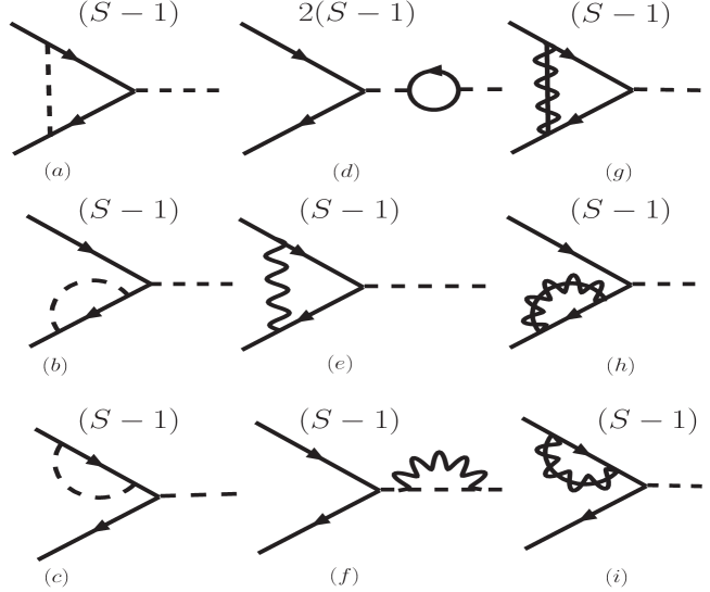
Figure 2: Diagrams contributing to Yukawa coupling evolution in the Landau gauge. Solid (broken) lines correspond to fermions (SM scalars), while wavy lines (wavy+solid lines) represent ordinary gauge bosons (fifth components of gauge bosons).

Figure 3: Evolution of the top quark Yukawa coupling in the UED scenario (left panel) and (b) the SM (right panel). UED evolution is shown for three different values of $R^{-1}$ and the curves are terminated at the corresponding unification scales.

The Feynman diagrams that contribute to the power law evolution of Yukawa couplings (in Landau gauge) are shown in Fig. 2. The contributions come from the pure SM states, their KK towers, and from the adjoint representation scalars. The last two contributions, as the master formula (2) indicates, have an overall proportionality factor $(S-1)$. As we examine contributions from individual KK states, we see that due to the argument of fermion chirality, not in all diagrams do the cosine and sine mode states both simultaneously contribute. This accounts for a relative factor of 2 between the two types of diagrams. For example, in Fig. 2a the fermionic KK modes can only come from cosine expansions, whereas in Fig. 2d both cosine and sine fermion modes contribute. This is why Fig. 2a has a multiplicating factor $(S-1)$, while for Fig. 2d the factor is $2(S-1)$. Whereever $A_{5}$ is involved as an internal line, the associated KK internal fermions necessarily come from sine expansion, e.g. in Figs. 2g, 2h and 2i. The above book-keeping has been done for individual graphs and the proportionality factors have been mentioned for each diagram in Fig. 2. The Yukawa RG equations (beyond the threshold $R^{-1}$) can be written as ($t=\ln E$):

$$16\pi^{2}\frac{dy_{f}}{dt}=\beta^{\rm SM}_{y_{f}}+\beta^{\rm UED}_{y_{f}},$$ (4)

where $f$ generically stands for the up/down quarks or leptons. The SM beta functions $\beta^{\rm SM}_{y_{f}}$ can be found e.g. in [18]. The UED contributions to the beta functions $\beta^{\rm UED}_{y_{l,u,d}}$ are given by: $\displaystyle\beta^{\rm UED}_{y_{l}}$ $\displaystyle=$ $\displaystyle(S-1)\;\left[-(\frac{21}{8}g_{2}^{2}+\frac{129}{40}g_{1}^{2})+\frac{3}{2}y_{l}^{2}\right]\;y_{l}+2(S-1)\;\left[Y_{l}+3Y_{u}+3Y_{d}\right]\;y_{l},$ $\displaystyle\beta^{\rm UED}_{y_{u}}$ $\displaystyle=$ $\displaystyle(S-1)\;\left[-(12g_{3}^{2}+\frac{21}{8}g_{2}^{2}+\frac{9}{8}g_{1}^{2})+\frac{3}{2}(y_{u}^{2}-y_{d}^{2})\right]\;y_{u}+2(S-1)\;\left[Y_{l}+3Y_{u}+3Y_{d}\right]\;y_{u},$ (5) $\displaystyle\beta^{\rm UED}_{y_{d}}$ $\displaystyle=$ $\displaystyle(S-1)\;\left[-(12g_{3}^{2}+\frac{21}{8}g_{2}^{2}+\frac{9}{40}g_{1}^{2})+\frac{3}{2}(y_{d}^{2}-y_{u}^{2})\right]\;y_{d}+2(S-1)\;\left[Y_{l}+3Y_{u}+3Y_{d}\right]\;y_{d},$ with $Y_{l}=\sum_{l}y_{l}^{2}$, $Y_{d}=\sum_{d}y_{d}^{2}$, and $Y_{u}=\sum_{u}y_{u}^{2}$. To illustrate how the power law dependence of Yukawa couplings quantitatively compares and contrasts with their 4-dimensional logarithmic running, we have exhibited in Fig. 3 the behaviour of the top-quark Yukawa coupling in the two cases.

Another consequence of unification in many models is a prediction of the low energy value of $m_{b}/m_{\tau}$. This ratio, unity at the unification scale, at low energies takes the values 4.7, 4.2, and 3.9 for $1/R$ = 1, 5, and 20 TeV, respectively. Admittedly, $m_{b}$ is on the high side; a limitation which perhaps may be attributable to the one-loop level of the calculation.

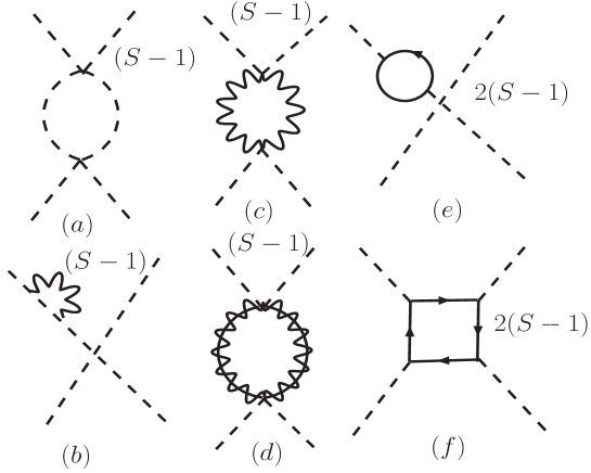
Figure 4: Diagrams contributing to quartic scalar coupling evolution. The conventions are the same as in Fig. 2.

Figure 5: Bounds on the Higgs mass at the electroweak scale in the UED scenario from the triviality and vacuum stability conditions for $R^{-1}$ = 1, 5, and 20 TeV. See text for details.

III.3 Quartic scalar coupling and the Higgs mass

The one-loop diagrams through which the KK modes contribute to the power law running of the quartic scalar coupling $\lambda$ (in Landau gauge) are shown in Fig. 4. As clarified before in the case of Yukawa running, the extra factor of 2 in front of $(S-1)$ for some graphs indicates that cosine and sine KK modes both contribute only to those graphs. The evolution equation can be written as

$$16\pi^{2}\frac{d\lambda}{dt}=\beta^{\rm SM}_{\lambda}+\beta^{\rm UED}_{\lambda}$$ (6)

The expressions for $\beta^{\rm SM}_{\lambda}$ can be found e.g. in [19]. The UED beta functions are given by $\displaystyle\beta^{\rm UED}_{\lambda}$ $\displaystyle=$ $\displaystyle(S-1)\left[3g_{2}^{4}+\frac{6}{5}g_{2}^{2}g_{1}^{2}+\frac{9}{25}g_{1}^{4}-3\lambda(3g_{2}^{2}+\frac{3}{5}g_{1}^{2})+12\lambda^{2}\right]$ (7) $\displaystyle+$ $\displaystyle 2(S-1)\left[4\left(Y_{l}+3Y_{u}+3Y_{d}\right)\lambda-4\sum_{l,u,d}\left(y_{l}^{4}+3y_{u}^{4}+3y_{d}^{4}\right)\right].$ The evolution of $\lambda$ has interesting bearings on the Higgs mass. In the standard 4-dimensional context, bounds on the Higgs mass have been placed on the grounds of ‘triviality’ and ‘vacuum stability’ [20]. What do they imply in the UED context? The ‘triviality’ argument requires that $\lambda$ stays away from the Landau pole, i.e. remains finite, all the way to the cutoff scale $\Lambda$. The condition that $1/\lambda(\Lambda)>0$ can be translated to an upper bound on the Higgs mass ($m_{H}$) at the electroweak scale when the cutoff of the theory is $\Lambda$. This has been plotted in Fig. 5 (the upper curves) for three different values of $R$. A given point on that curve (for a given $R$) corresponds to a maximum allowed $m_{H}$ at the weak scale; for a larger $m_{H}$ the coupling $\lambda$ becomes infinite at some scale less than $\Lambda$ and the theory ceases to be perturbative. Clearly, this $m_{H}^{\rm max}$ varies as we vary the cutoff $\Lambda$ . The argument of ‘vacuum stability’ relies on the requirement that the scalar potential be always bounded from below, i.e. $\lambda(\Lambda)>0$. This can be translated to a lower bound $m_{H}^{\rm min}$ at the weak scale. The lower set of curves in Fig. 5 (for three values of $R^{-1}$) represent the ‘vacuum stability’ limits, the region below the curve for a given $R$ being ruled out. Recalling that the cutoff is where the gauge couplings tend to unify, we observe that the Higgs mass is limited in the narrow zone

$$148~{}\raisebox{-1.72218pt}{\hbox to0.0pt{$\sim$\hss}}\raisebox{1.72218pt}{$<$}~{}m_{H}~{}\raisebox{-1.72218pt}{\hbox to0.0pt{$\sim$\hss}}\raisebox{1.72218pt}{$<$}~{}186~{}{\rm GeV}$$ (8)

in all the three cases, for a zero mode top quark mass of 174.2 GeV. Admittedly, our limits are based on one-loop corrections only. That the upper and lower limits are insensitive to the choice of $R$ is not difficult to understand, as what really counts is the number of KK states, given by the product $\Lambda R$, which, as mentioned before, is nearly constant, order $\ln(10^{15})$. The limits in Eq. (8) are very close to what we obtain in the SM at the one-loop level, namely $147~{}\raisebox{-1.72218pt}{\hbox to0.0pt{$\sim$\hss}}\raisebox{1.72218pt}{$<$}~{}m_{H}^{\rm SM}~{}\raisebox{-1.72218pt}{\hbox to0.0pt{$\sim$\hss}}\raisebox{1.72218pt}{$<$}189$ GeV (see also [21], where one-loop SM results have been derived).

III.4 Supersymmetric UED

What happens if we take the supersymmetric (SUSY) version of UED? A 5-dimensional $N=1$ supersymmetry when perceived from a 4-dimensional context contains two different $N=1$ multiplets forming one $N=2$ supermultiplet. For a comprehensive analysis, we refer the readers to [5]. There are two issues that immediately concern our analysis. First, unlike in the non-SUSY case, the Higgs scalar in a chiral multiplet will now have both even and odd $Z_{2}$ modes on account of degrees of freedom counting consistent with supersymmetry. Also, there will be two such $N=2$ chiral supermultiplets to meet the requirement of supersymmetry. Second, in the RG evolution two energy scales will come into play. The first of these is the supersymmetry scale, called $M_{S}$, which we take to be 1 TeV. Beyond $M_{S}$, supersymmetric particles get excited and their contributions must be included in the RG evolution. The second scale is that of the compactified extra dimension $1/R$, which we take to be larger than $M_{S}$.

The gauge coupling evolution must now be specified for three different regions. The first of these is when $E<M_{S}$ where the SM with the additional scalar doublet beta functions are in control. In this region:

$${b}_{1o}=\frac{21}{5},~{}~{}{b}_{2o}=-\frac{10}{3},~{}~{}{b}_{3o}=-7.$$ (9)

Once $M_{S}$ is crossed and up until $1/R$, we also have the superpartners of the SM particles pitching in with their effects. The contributions of the SM particles and their superpartners together are given by:

$${b}_{1s}=\frac{33}{5},~{}~{}{b}_{2s}=1,~{}~{}{b}_{3s}=-3.$$ (10)

Finally, when the KK-modes are excited ($E>1/R$) one has further contributions from the individual modes:

$$\tilde{b}_{1}=\frac{66}{5},~{}~{}\tilde{b}_{2}=10,~{}~{}\tilde{b}_{3}=6.$$ (11)

Thus, beyond $1/R$, the total contribution is given by

$$b_{i}^{\rm tot}=b_{io}+\Theta(E-M_{S})~{}(b_{is}-b_{i0})+\Theta(E-\frac{1}{R})~{}(S-1)~{}\tilde{b}_{i},$$ (12)

Not unexpectedly, for the SUSY UED case, gauge unification is possible. We observe that the introduction of this plethora of KK excitations of the SM particles and their superpartners radically changes the beta functions; so much so, that the gauge couplings tend to become non-perturbative before unification is achieved. For clarity, we make the argument more explicit below. First, from Eqs. (10) and (11) we note that the dominance of the KK matter over the KK gauge parts is so overwhelming that the SU(3) beta function ($\tilde{b}_{3}$) beyond the first KK threshold ceases to be negative any longer. The other two gauge beta functions, which were already positive with contributions from zero mode particles plus their superpartners, become even more positive. So the curves for all the three gauge couplings would have the same sign slopes once the KK modes are excited. As a result, with increasing energy the three curves for $\alpha_{g}^{-1}$ would dip with a power law scaling fast into a region where the couplings themselves become too large at the time they meet. Therefore, in order that all of them remain perturbative during the entire RG evolution, the onset of the KK dynamics has to be sufficiently delayed. This requirement imposes $R^{-1}~{}\raisebox{-1.72218pt}{\hbox to0.0pt{$\sim$\hss}}\raisebox{1.72218pt}{$>$}~{}5.0\times 10^{10}$ GeV. In effect, this implies that the twin requirements of a SUSY-UED framework as well as perturbative gauge coupling unification pushes the detectability of the KK excitations well beyond the realm of the LHC.

IV Conclusions and Outlook

As the LHC is getting all set to roar in 2007, expectations are mounting as we prepare ourselves to get a glimpse of new and unexplored territory. New physics of different incarnations, especially supersymmetry and/or extra dimensions, are crying out for verification. How does the landscape beyond the electroweak scale confront the evolution of the gauge, Yukawa and scalar quartic couplings? Will there be a long logarithmic march through the desert all the way to $10^{(16-17)}$ GeV, or is a power law sprint awaiting us with a stamp of extra dimensions? In which way does the latter quantitatively differ from the former has been the subject of our investigation in the present paper. We observe the following landmarks that characterise the extra-dimensional running:

1. The orbifolding renders some subtle features to the RG running in UED. Due to the conservation of KK number at tree level vertices, the $Z_{2}$ even and odd KK states selectively contribute to different diagrams. While some diagrams are forbidden, there are new diagrams originating from adjoint scalar exchanges. In the present article we have performed a diagram by diagram book-keeping leading to the evolution equations.

2. Low gauge coupling unification scales can be achieved without introducing non-perturbative gauge couplings. The unification scale depends on $R$, and is approximately given by $\Lambda\sim(25-30)/R$.

3. The ‘triviality’ and ‘vacuum stability’ bounds on the Higgs mass have been studied in the context of power law evolution. This limits the Higgs mass in the range $148~{}\raisebox{-1.72218pt}{\hbox to0.0pt{$\sim$\hss}}\raisebox{1.72218pt}{$<$}m_{H}~{}\raisebox{-1.72218pt}{\hbox to0.0pt{$\sim$\hss}}\raisebox{1.72218pt}{$<$}186$ GeV at the one-loop level. The corresponding SM limits at the one-loop level are not very different.

4. If low energy SUSY is realised in Nature, then the requirement of perturbative gauge coupling unification pushes the inverse radius of compactification all the way up to $\sim 10^{10}$ GeV. Thus if superpartners of the SM particles are observed at the LHC, the nearest KK states within the UED framework are predicted to lie beyond the boundary of any observational relevance.

It should be admitted that even if TeV scale extra dimensional theories are established, the spectrum might be more complicated than what UED predicts. The confusion is expected to clear up at least when the low-lying KK states face appointment with destiny within the first few years of the LHC run. Our intention in the present article has been to choose a simple framework to study power law evolution. Flat extra dimensional models are particularly handy as they provide equispaced KK states which allow an elegant handling of internal KK summation in the loops. UED is an ideal test-bed to conduct this study as it has been motivated from various angles and subjected to different phenomenological tests.

Acknowledgements:  We thank E. Dudas for useful correspondences. G. B. thanks CFTP, Instituto Superior Técnico (Lisbon) and ICTP (Trieste) for hospitality at different stages of the work.

References

- [1] I. Antoniadis, Phys. Lett. B 246 (1990) 377.
- [2] N. Arkani-Hamed and M. Schmaltz, Phys. Rev. D 61 (2000) 033005 [arXiv:hep-ph/9903417].
- [3] G. Servant and T. M. P. Tait, Nucl. Phys. B 650 (2003) 391 [arXiv:hep-ph/0206071].
- [4] N. Arkani-Hamed, H. C. Cheng, B. A. Dobrescu and L. J. Hall, Phys. Rev. D 62 (2000) 096006 [arXiv:hep-ph/0006238].
- [5] K. Dienes, E. Dudas, and T. Gherghetta; Nucl. Phys. B 537 (1999) 47 [arXiv:hep-ph/9806292].
- [6] K. R. Dienes, E. Dudas and T. Gherghetta, Phys. Lett. B 436 (1998) 55 [arXiv:hep-ph/9803466]. For a parallel analysis based on a minimal length scenario, see S. Hossenfelder, Phys. Rev. D 70 (2004) 105003 [arXiv:hep-ph/0405127].
- [7] T. Appelquist, H. C. Cheng and B. A. Dobrescu, Phys. Rev. D 64 (2001) 035002 [arXiv:hep-ph/0012100].
- [8] P. Nath and M. Yamaguchi, Phys. Rev. D 60 (1999) 116006 [arXiv:hep-ph/9903298].
- [9] D. Chakraverty, K. Huitu and A. Kundu, Phys. Lett. B 558 (2003) 173 [arXiv:hep-ph/0212047].
- [10] A.J. Buras, M. Spranger and A. Weiler, Nucl. Phys. B 660 (2003) 225 [arXiv:hep-ph/0212143]; A.J. Buras, A. Poschenrieder, M. Spranger and A. Weiler, Nucl. Phys. B 678 (2004) 455 [arXiv:hep-ph/0306158].
- [11] K. Agashe, N.G. Deshpande and G.H. Wu, Phys. Lett. B 514 (2001) 309 [arXiv:hep-ph/0105084].
- [12] J.F. Oliver, J. Papavassiliou and A. Santamaria, Phys. Rev. D 67 (2003) 056002 [arXiv:hep-ph/0212391].
- [13] T. Appelquist and H. U. Yee, Phys. Rev. D 67 (2003) 055002 [arXiv:hep-ph/0211023].
- [14] T.G. Rizzo and J.D. Wells, Phys. Rev. D 61 (2000) 016007 [arXiv:hep-ph/9906234]; A. Strumia, Phys. Lett. B 466 (1999) 107 [arXiv:hep-ph/9906266]; C.D. Carone, Phys. Rev. D 61 (2000) 015008 [arXiv:hep-ph/9907362].
- [15] T. Rizzo, Phys. Rev. D 64 (2001) 095010 [arXiv:hep-ph/0106336]; C. Macesanu, C.D. McMullen and S. Nandi, Phys. Rev. D 66 (2002) 015009 [arXiv:hep-ph/0201300]; Phys. Lett. B 546 (2002) 253 [arXiv:hep-ph/0207269]; H.-C. Cheng, Int. J. Mod. Phys. A 18 (2003) 2779 [arXiv:hep-ph/0206035]; A. Muck, A. Pilaftsis and R. Rückl, Nucl. Phys. B 687 (2004) 55 [arXiv:hep-ph/0312186].
- [16] P. Dey and G. Bhattacharyya, Phys. Rev. D 70 (2004) 116012 [arXiv:hep-ph/0407314]; P. Dey and G. Bhattacharyya, Phys. Rev. D 69 (2004) 076009 [arXiv:hep-ph/0309110].
- [17] T. Appelquist, B. A. Dobrescu, E. Ponton and H. U. Yee, Phys. Rev. Lett. 87 (2001) 181802 [arXiv:hep-ph/0107056]; R. N. Mohapatra and A. Perez-Lorenzana, Phys. Rev. D 67 (2003) 075015 [arXiv:hep-ph/0212254].
- [18] C. Hill, C. N. Leung, and S. Rao; Nucl. Phys. B 262 (1985) 517.
- [19] T. P. Cheng, E. Eichten, and L. F. Li; Phys. Rev. D 9 (1974) 2259.
- [20] G. Altarelli and G. Isidori, Phys. Lett. B 337 (1994) 141; S. Dawson, arXiv:hep-ph/9901280.
- [21] P. Kielanowski and S. R. Juarez W., Phys. Rev. D 72 (2005) 096003 [arXiv:hep-ph/0310122].