Lepton flavor violation in muonium decay and muon colliders
in models with heavy neutrinos

Abstract

We study the lepton-flavor-violating reaction $\mu^{+}e^{-}\to e^{+}e^{-}$ within two extensions of the standard model that include heavy neutrinos. The reaction is studied in the low energy limit in the form of muonium decay $M\to e^{+}e^{-}$ and in the high energy regime of a muon collider. The two theoretical models we consider are: model I, a typical see-saw model that violates lepton flavor and number by inclusion of extra right handed neutrinos, and model II, a variant where lepton number is conserved and which includes extra right handed as well as left handed neutrinos, singlets under the gauge group. We find for muonium decay into $e^{+}e^{-}$ the extremely small result $Br(M\to e^{+}e^{-})<10^{-19}$ in both scenarios. Alternatively, for $\mu^{+}e^{-}$ collisions up to $\sqrt{s}\sim 50$ GeV we find $\sigma(\mu^{+}e^{-}\to e^{+}e^{-})<10^{-5}$ fb, while for energies above the $W^{+}W^{-}$ threshold we find $\sigma(\mu^{+}e^{-}\to W^{+}W^{-})$ up to $\sim 1$ fb.

I Introduction

A current issue in particle physics is the understanding of the neutrino sector. It is by now consistent with experimental results to assert that at least some of the standard neutrinos must have small (but non-zero) masses and these mass states should mix under the weak interactionsFogli . As a consequence, the lightness of the standard neutrinos ($m_{\nu}\lesssim 1$ eV) compared to the charged leptons ($\gtrsim$ MeV) remains to be understood. If neutrinos are of a Dirac nature, non-zero masses can appear in the standard model (SM) by inclusion of (sterile) right-handed neutrinosSchechter . If neutrinos are of a Majorana nature –a more general case–, more appealing solutions exist in the context of extended gauge structures. An interesting solution is provided by the so-called seesaw mechanism within $SO(10)$ or left-right symmetric models of interactions. In conventional seesaw models, the effective light neutrino masses are within the scales of eV to MeV via a relation involving the hierarchy between very large Majorana masses and Dirac masses comparable to those of the charged leptonsSeesaw . Another possible solution was investigated in the framework of heterotic superstring models E6 with $E_{6}$ symmetry or certain scenarios of $SO(10)$ models SO10a , where the low–energy effective theories include new left–handed and right–handed neutral isosinglets and assume conservation of total lepton number in the Yukawa sector.

One avenue to study the neutrino sector is to consider lepton flavor violating processes (LFV) of standard particles, which are absent in the SM and depend on neutrino masses and mixings. Free lepton decays like $\mu\to e\gamma$ $\mu\to 3e$, $\tau\to 3\mu$, etc. are among the most direct LFV processes and they have been studied in detail Lee -Kageyama ,CDKK . Other ways like muon-to-electron conversion in nuclei and muonium-to-antimuonium conversion are also possibilities muonium ; Willmann ; CDKK2 . Yet another possibility is to consider lepton-lepton scattering or bound state decays (e.g. muonium decay). These modes contain the same underlying physics as free lepton decays, but differ in the experimental conditions and, from the phenomenological viewpoint they are sensitive to other combination of parameters because of their different kinematical regime.

In this work we study the process $\mu^{+}e^{-}\to e^{+}e^{-}$ at low energy in the form of muonium decay (muonium is a non-relativistic $\mu^{+}e^{-}$ bound state) and at high energy in the form of $\mu^{+}e^{-}$ collisions. Muonium is formed when a $\mu^{+}$ slows down inside a material and captures an electron, forming a bound state due to Coulomb attraction. The fraction of muons that actually end up as muonium depends very much on the material, ranging from small fractions in some to nearly 100% in others. Most muonia decay as $M\to e^{+}e^{-}\bar{\nu}_{\mu}\nu_{e}$, which is simply a muon decay with an electron as spectator Czarnecki . A more rare mode, albeit standard, is annihilation $M\to\bar{\nu}_{\mu}\nu_{e}$, whose rate is $\sim 10^{-11}$ times smaller. Here we study the mode $M\to e^{+}e^{-}$, which violates lepton flavor and is thus forbidden in the SM. From our point of view, muonium decay is interesting because it is a non-relativistic $\mu^{+}e^{-}$ process, and thus depends on different combinations of parameters than in high energy processes. Complementary to it, we also study the collision $\mu^{+}e^{-}\to e^{+}e^{-}$ at high energy. This process clearly requires a muon collider. We will not be exhaustive in the study of new physics at muon colliders but focus on this particular channel within the LFV models previously mentioned. In section II we give a brief review of the seesaw type models in question; in section III we describe the generic amplitudes for $\mu^{+}e^{-}\to e^{+}e^{-}$ processes within these models; section IV contains the application to muonium decay, section V the application to high energy collisions and section VI summarizes the results and conclusions.

II Two Models for heavy neutrinos

Here we will briefly summarize the two models under consideration. Further details were given in previous worksCDKK ; CDKK2 . The main features of these models are (i) they contain heavy neutrinos, (ii) in the mass eigenstate basis, the heavy neutrinos couple with charged leptons of mixed flavor under weak interactions (just like Cabbibo-Kobayashi-Maskawa mixing in the quark sector), and (iii) the neutrinos are generally of Majorana type.

Model I:  This is a usual seesaw model Seesaw : it is the standard model with $N_{L}$ generations (i.e. left-handed neutrinos $\nu_{iL}$) and an equal number $N_{H}=N_{L}$ of right-handed neutrinos ${\widetilde{\nu}}_{iR}$, singlets under the gauge group. The neutrino mass terms, after gauge symmetry breaking, are:

$$-{\cal L}^{\nu}_{\rm mass}=\frac{1}{2}\left({\overline{{\nu}_{L}}},{\overline{{\widetilde{\nu}}_{R}^{\ c}}}\right){\cal M}\left(\begin{array}[]{c}\nu_{L}^{\ c}\\ {\widetilde{\nu}}_{R}\end{array}\right)+{\rm h.c.}$$ (1)

The superscript $c$ at some of the fields denotes charge-conjugated fields $\psi^{c}={\cal C}{\overline{\psi}}^{T}$, where ${\cal C}=-i\gamma^{2}\gamma^{0}$ in the Dirac representation. The $2N_{L}\times 2N_{L}$–dimensional matrix ${\cal M}$ has a seesaw block form:

$${\cal M}=\left(\begin{array}[]{cc}0&m_{D}\\ m_{D}^{T}&m_{M}\end{array}\right),\quad m_{D}=\left(\begin{array}[]{cc}a&b\;e^{i\delta_{1}}\\ c\;e^{i\delta_{2}}&d\end{array}\right),\quad m_{M}=\left(\begin{array}[]{cc}M_{1}&0\\ 0&M_{2}\end{array}\right)\ ,$$ (2)

The (real) parameters $a$, $b$, $c$, $d$ in the Dirac mass matrix $m_{D}$ are smaller than the Majorana mass parameters $M_{1}$ and $M_{2}$ ($M_{2}\geq M_{1}\gtrsim 100$ GeV) by at least an order of magnitude.

The squared ratio between the Dirac mass ($m_{D}$) and the Majorana mass ($m_{M}$) scales gives the order of magnitude of the heavy-to-light neutrino mixings $(s_{L}^{\nu_{l}})^{2}\equiv\sum_{h}|U_{hl}|^{2}\sim|m_{D}|^{2}/|m_{M}|^{2}$. The physical light neutrino masses are of the order of $m_{\nu_{light}}\!\sim\!m^{2}_{D}/m_{M}$. The very low experimental bounds $m_{\nu_{light}}\stackrel{{\scriptstyle<}}{{\sim}}1$ eV impose in Model I severe constraints on the $|m_{D}|\ll|m_{M}|$ hierarchy required. The present experimental bounds on the heavy-to-light mixing parameters $(s_{L}^{\nu_{l}})^{2}\sim|m_{D}|^{2}/|m_{M}|^{2}$ ($\stackrel{{\scriptstyle<}}{{\sim}}10^{-2}$, see below) present another set of constraints on the model.

Model II:   This model contains an equal number $N_{L}$ of left-handed ($S_{iL}$) and right-handed (${\widetilde{\nu}}_{iR}$) neutral singlets E6 ; SO10a . Furthermore, the form of the mass matrix ${\cal M}$ leads to the conservation of total Lepton Number, although lepton flavor mixing is still possible. The neutrino mass terms, after electroweak symmetry breaking, have the form

$$-{\cal L}^{\nu}_{\rm mass}=\frac{1}{2}\left({\overline{{\nu}_{L}}},{\overline{{\widetilde{\nu}}_{R}^{\ c}}},{\overline{{S}_{L}}}\right){\cal M}\left(\begin{array}[]{c}{\nu_{L}^{\ c}}\\ {\widetilde{\nu}}_{R}\\ S_{L}^{\ c}\end{array}\right)+{\rm h.c.}\ ,\qquad{\cal M}=\left(\begin{array}[]{ccc}0&m_{D}&0\\ m_{D}^{T}&0&m_{M}^{T}\\ 0&m_{M}&0\end{array}\right)\ ,$$ (3)

and $m_{D}$ and $m_{M}$ are given in Eq. (2). The mass matrix ${\cal M}$ is $(N_{L}+N_{H})\times(N_{L}+N_{H})$-dimensional, $N_{H}=2N_{L}$ (the Dirac block $m_{D}$ is $N_{L}\times N_{L}$–dimensional). The model, in its unperturbed form, predicts for each of the $N_{L}$ generations a massless Weyl neutrino and two degenerate Majorana neutrinos  BRV ; Gonzalez-Garcia:1989rw ($N_{H}=2N_{L}$). Therefore, the seesaw-type restriction $m_{\nu_{light}}\!\sim\!m^{2}_{D}/m_{M}$ of Model I is not present in Model II in its unperturbed form. However, present experimental bounds on heavy-to-light mixing parameters $(s_{L}^{\nu_{l}})^{2}\sim|m_{D}|^{2}/|m_{M}|^{2}$ ($\stackrel{{\scriptstyle<}}{{\sim}}10^{-2}$) do impose a certain level of hierarchy $|m_{D}|<|m_{M}|$ between the Dirac and Majorana mass sector, but is in general significantly weaker than in Model I. Nonzero masses of the $N_{L}$ light neutrinos can be generated in Model II by introducing small perturbations in the lower right block of ${\cal M}$, i.e., small Majorana mass terms for the neutral singlets $S_{iL}$, and this does not significantly affect the mixings of heavy-to-light neutrinos.

In either model, the mass matrix ${\cal M}$ can always be diagonalized by means of a congruent transformation involving a unitary matrix $U$

$$U{\cal M}U^{T}\Lambda^{*} = {\cal M}_{d}\ ,$$ (4)

where ${\cal M}_{d}={\rm diag}(m_{1},m_{2},\ldots)$ is the nonnegative diagonal mass matrix, and $\Lambda^{*}$ is an arbitrary diagonal unitary matrix: $(\Lambda^{*})_{ij}=\delta_{ij}\lambda^{*}_{i}$ and $|\lambda_{i}|=1$. The $N_{L}+N_{H}$ mass eigenstates $n_{i}$ are Majorana neutrinos, and are related to the interaction eigenstates $\nu_{kL}$ and ${\widetilde{\nu}}_{jR}$ by the matrices $U$ and $\Lambda^{\ast}$ as:

$$\left(\begin{array}[]{c}\nu_{L}\\ {\widetilde{\nu}}_{R}^{\ c}\end{array}\right)_{a} = \sum^{N_{L}+N_{H}}_{i=1}U^{*}_{ia}~{}{n_{iL}}\quad\Rightarrow\ \quad\left(\begin{array}[]{c}\nu_{L}^{\ c}\\ {\widetilde{\nu}}_{R}\end{array}\right)_{a}=\sum^{N_{L}+N_{H}}_{i=1}U_{ia}~{}\lambda^{*}_{i}~{}{n_{iR}}\ ,$$ (9)

The first $N_{L}$ eigenstates $n_{i}$ ($i=1,\ldots,N_{L}$) are the light partners of the standard charged leptons. The other $N_{H}$ eigenstates are heavy. It can be checked from relations (9) that the relation $(n_{iL})^{c}=\lambda_{i}^{*}n_{iR}$ holds, and thus $\lambda_{i}$ is recognized as the creation phase factor Kayser:1984ge ; Kayserb of the Majorana neutrino $n_{i}$.

In the mass basis, a $N_{L}\times(N_{L}\!+\!N_{H})$-dimensional mixing matrix $B$ for charged current interactions, and a $(N_{L}\!+\!N_{H})\times(N_{L}\!+\!N_{H})$-dimensional matrix $C$ for neutral current interactions can be introduced:

$$B_{li}=U^{*}_{il},\qquad C_{ij}=\sum^{N_{L}}_{a=1}U_{ia}U^{*}_{ja}\ .$$ (10)

Accordingly, the leptonic weak interactions are (cf. Pilaftsis:1991ug ; CDKK2 )

$${\cal L}_{lnW}(x) = \left(-\frac{g_{w}}{\sqrt{2}}\right)W_{\mu}^{-}(x)\;\sum_{i=1}^{N_{L}}\sum_{j=1}^{N_{L}+N_{H}}B_{ij}{\overline{l}}_{i}(x)\gamma^{\mu}P_{L}n_{j}(x)+{\rm h.c.}\ ,$$ (11)

$${\cal L}_{lnG}(x) = \left(-\frac{g_{w}}{\sqrt{2}M_{W}}\right)G^{-}(x)\sum_{i=1}^{N_{L}}\sum_{j=1}^{N_{L}+N_{H}}B_{ij}{\overline{l}}_{i}(x)\left(m_{li}\,P_{L}-m_{j}P_{R}\right)n_{j}(x)+{\rm h.c.}\ ,$$ (12)

$${\cal L}_{nnZ}(x) = \left(-\frac{g_{w}}{4}\frac{M_{Z}}{M_{W}}\right)Z^{0}_{\mu}(x)\;\sum_{i,j=1}^{N_{L}+N_{H}}{\overline{n}}_{i}(x)\gamma^{\mu}\left(C_{ij}P_{L}-C_{ij}^{\ast}P_{R}\right)n_{j}(x)+{\rm h.c.}\ ,$$ (13)

$${\cal L}_{nnG}(x) = \frac{ig_{w}}{4M_{W}}G^{0}(x)\sum_{i,j=1}^{N_{L}+N_{H}}{\overline{n}}_{i}(x)\left\{i\ (m_{j}-m_{i}){\rm Im}C_{ij}+\gamma_{5}(m_{j}+m_{i}){\rm Re}C_{ij}\right\}n_{j}(x)\ ,$$ (14)

where $G^{-}$ and $G^{0}$ are the Goldstone bosons that appear in a general gauge. Here, the conventions of Itzykson and ZuberIZ are used; $P_{L}=(1-\gamma_{5})/2$, $P_{R}=(1+\gamma_{5})/2$; $l_{i}$ is the $i$-th negatively charged lepton ($l_{1}=e^{-}$, $l_{2}=\mu^{-}$); $g_{w}$ is the $SU(2)_{L}$ coupling constant ($g_{w}^{2}=8G_{F}M_{W}^{2}/\sqrt{2}$) and $n_{j}$ are the Majorana neutrinos (mass eigenstates).

In all our numerical calculations we will just use two generations (i.e. $N_{L}=2$), since a third generation does not make a sizable change in our results, considering the uncertainties involved.

III Transition amplitude for $\mu^{+}e^{-}\to e^{+}e^{-}$

The amplitude for this process is similar to those of Ref. IP for lepton decays. Just as in that case, the amplitude for $\mu^{+}e^{-}\to e^{+}e^{-}$ can be calculated neglecting external momenta and external masses inside the loop, provided the neutrinos in the loop are heavy. Let us define the kinematics of the process as:

$$\mu^{+}(k_{1})\ e^{-}(k_{2})\ \to\ e^{+}(k_{3})\ e^{-}(k_{4}).$$ (15)

The transition amplitude is a sum of photon- and Z- penguin diagrams (Fig. 1) and box diagrams (Fig. 2). There are two types of penguin diagrams in each case: those where the photon or Z is in the t-channel and those where it is in the s-channel (see Fig. 1). There is a relative minus sign between those diagrams due to Fermi statistics. The contribution to the amplitude from the photon penguins has two form factors, $F_{\gamma}^{e\mu}$ and $G_{\gamma}^{e\mu}$ IP :

$$i{\cal T}_{\gamma} = i\frac{\alpha_{w}^{2}\sin^{2}\theta_{w}}{2M_{W}^{2}}{\Bigg{\{}}\left[{\overline{v}}_{\mu}(k_{1})\left(F_{\gamma}^{e\mu}\ \big{(}\gamma^{\rho}-\frac{q^{\rho}{q\hbox to0.0pt{\hss/}}}{q^{2}}\big{)}P_{L}\ -\ iG_{\gamma}^{e\mu}\ \frac{\sigma_{\rho\sigma}q^{\sigma}}{q^{2}}(m_{e}P_{R}+m_{\mu}P_{L})\right)u_{e}(k_{2})\right]\times\Big{[}{\overline{u}}_{e}(k_{4})\gamma_{\rho}v_{e}(k_{3})\Big{]}$$ (16)

$$\qquad\qquad\qquad-\quad\Big{[}v_{e}(k_{3})\leftrightarrow u_{e}(k_{2}),\quad q\to q^{\prime}\Big{]}{\Bigg{\}}}\ ,\qquad(q=k_{1}+k_{2},\quad q^{\prime}=k_{1}-k_{3})\ .$$

where $\alpha_{w}=g^{2}/(4\pi)$, $P_{R/L}=(1\pm\gamma_{5})/2$ are the chiral projectors, and $\sigma_{\rho\sigma}=(i/2)[\gamma_{\rho},\gamma_{\sigma}]$. The term $q^{\rho}{q\hbox to0.0pt{\hss/}}$ vanishes when contracted to the vector current of the $e^{+}e^{-}$ pair. Similarly, the Z penguins contain one form factor $F_{Z}^{e\mu}$:

$$i{\cal T}_{Z} = i\frac{\alpha_{w}^{2}}{4M_{W}^{2}}{\Bigg{\{}}F_{Z}^{e\mu}\ \Big{[}{\overline{v}}_{\mu}(k_{1})\gamma^{\rho}P_{L}u_{e}(k_{2})\Big{]}\times\Big{[}{\overline{u}}_{e}(k_{4})\gamma_{\rho}\left((1-2\sin^{2}\theta_{w})P_{L}-2\sin^{2}\theta_{w}P_{R}\right)v_{e}(k_{3})\Big{]}$$ (17)

$$\qquad\qquad\qquad-\ \Big{[}v_{e}(k_{3})\leftrightarrow u_{e}(k_{2})\Big{]}{\Bigg{\}}}\ ,$$

and the box diagrams also one form factor, $F_{B}^{e\mu ee}$:

$$i{\cal T}_{{\rm Box}}\ =\ i\frac{\alpha_{w}^{2}}{4M_{W}^{2}}F_{B}^{e\mu ee}\Big{[}{\overline{v}}_{\mu}(k_{1})\gamma^{\rho}P_{L}u_{e}(k_{2})\Big{]}\times\Big{[}{\overline{u}}_{e}(k_{4})\gamma_{\rho}P_{L}v_{e}(k_{3})\Big{]}\ .$$ (18)

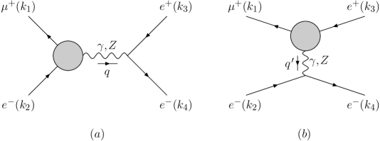
Figure 1: The one-loop penguin diagrams for $\mu^{+}(k_{1})e^{-}(k_{2})\to e^{+}(k_{3})e^{-}(k_{4})$: (a) s-channel penguin and (b) t-channel penguin. The blob represents the loop involving $W,G$ bosons and neutrinos. The diagram (b), i.e. t-channel, corresponds to the contributions in the last lines of Eqs. (16) and (17).

Figure 2: The box diagrams for $\mu^{+}(k_{1})e^{-}(k_{2})\to e^{+}(k_{3})e^{-}(k_{4})$. The diagrams (b) and (d) are obtained from (a) and (c), respectively, by the exchange $e^{-}(k_{2})\leftrightarrow e^{+}(k_{3})$ and by the corresponding change in the flow of time.

The form factors $F_{\gamma}^{e\mu}$, $G_{\gamma}^{e\mu}$, $F_{Z}^{e\mu}$ and $F_{B}^{e\mu ee}$ are

$$F^{e\mu}_{\gamma} = \sum^{N_{L}+N_{H}}_{i=1}B^{*}_{ei}B_{\mu i}\ F_{\gamma}(x_{i})\approx\sum_{I>N_{L}}B^{*}_{eI}B_{\mu I}F_{\gamma}(x_{I})\ ,$$ (19)

$$G^{e\mu}_{\gamma} = \sum^{N_{L}+N_{H}}_{i=1}B^{*}_{ei}B_{\mu i}\ G_{\gamma}(x_{i})\approx\sum_{I>N_{L}}B^{*}_{eI}B_{\mu I}G_{\gamma}(x_{I})\ ,$$ (20)

$$F^{e\mu}_{Z} = \sum^{N_{L}+N_{H}}_{i,j=1}B^{*}_{ei}B_{\mu j}\Big{[}\delta_{ij}\ F_{Z}(x_{i})+C_{ij}\ H_{Z}(x_{i},x_{j})+C^{*}_{ij}\ G_{Z}(x_{i},x_{j})\Big{]}$$ (22)

$$\approx \sum_{I>N_{L}}B^{*}_{eI}B_{\mu I}F_{Z}(x_{I})+\sum_{I,J>N_{L}}B^{*}_{eI}B_{\mu J}\left[C_{IJ}H_{Z}(x_{I},x_{J})+C^{*}_{IJ}\left(G_{Z}(x_{I},x_{J})-G_{Z}(x_{I},0)-G_{Z}(0,x_{J})\right)\right]$$

$$+2\sum_{I>N_{L}}B^{*}_{eI}B_{\mu I}G_{Z}(x_{I},0)\ ,$$

$$F^{e\mu ee}_{B} = \sum^{N_{L}+N_{H}}_{i,j=1}\Big{[}2|B_{ei}|^{2}B^{*}_{ej}B_{\mu j}\ F_{\rm Box}(x_{i},x_{j})-(B^{*}_{ei})^{2}B_{ej}B_{\mu j}\lambda_{j}\lambda^{*}_{i}\ G_{\rm Box}(x_{i},x_{j})\Big{]}$$ (24)

$$\approx 2\sum_{I,J>N_{L}}|B_{eI}|^{2}B^{*}_{eJ}B_{\mu J}\left[F_{\rm Box}(x_{I},x_{J})+F_{\rm Box}(0,0)-F_{\rm Box}(x_{I},0)-F_{\rm Box}(0,x_{J})\right]$$

$$-\sum_{I,J>N_{L}}(B^{*}_{eI})^{2}B_{eJ}B_{\mu J}\lambda_{J}\lambda^{*}_{I}\ G_{\rm Box}(x_{I},x_{J})+2\sum_{J>N_{L}}B^{*}_{eJ}B_{\mu J}\left(F_{\rm Box}(0,x_{J})-F_{\rm Box}(0,0)\right)\ ,$$

where $x_{i}=m_{i}^{2}/M_{W}^{2}$ ($m_{i}$ is the mass of the Majorana neutrino of type $i$ inside the loop), and the functions $F_{\gamma}(x)$, $G_{\gamma}(x)$, $F_{Z}(x)$, $H_{Z}(x,y)$, $G_{Z}(x,y)$, $F_{\rm Box}(x,y)$ and $G_{\rm Box}(x,y)$ appear from the loop integrals IP , in the approximation where external masses and momenta are neglected. The explicit expressions of these functions are given in Ref. CDKK2 . $F_{\rm Box}$ corresponds to the diagrams of Figs. 2(a) and (b), and $G_{\rm Box}$ to those of Figs. 2(c) and (d) which exist only for Majorana neutrinos. Eqs. (19)-(24) involve summation over all 2-component neutrinos, where $N_{L}$ is the number of standard (light) ones and $N_{H}$ the number of extra (heavy) ones ($=\!N_{L},2N_{L}$ in Models I, II, respectively). All these expressions are identical to those obtained in Ref. IP for neutrinoless lepton decays, except for the sign in front of the term proportional to $G_{\rm Box}(x_{i},x_{j})$ – for details on the latter point, cf. Ref. CDKK2 . Furthermore, in Eqs. (19)-(24) the expressions in a modified form are included which involve only the light-to-heavy mixing elements $B_{\ell I}$ ($\ell\leq N_{L};I>N_{L}$); they are obtained by taking into account the unitarity of the $U$ matrix, and the fact that the light neutrino masses are $m_{\ell}\ll M_{W}$.

The parameters $\lambda_{i}$ are the creation phase factorsKayserb of the Majorana neutrinos $n_{i}$ and $n_{j}$, respectively ($n_{j}^{c}=\lambda_{j}^{\ast}n_{j}$), which appear in the matrix $\Lambda$ of Eq. (4). In the case of no CP violation and real mass matrix ${\cal M}$, we can choose the unitary matrix $U$ as a real orthogonal matrix which diagonalizes the symmetric and real matrix ${\cal M}$; then some of the $\lambda_{j}$’s are $+1$ and others are $-1$ CDKK2 . Nonetheless we can choose all $\lambda_{j}=+1$, but then in general the unitary matrix $U$ will not be real.

The total amplitude for $\mu^{+}e^{-}\to e^{+}e^{-}$ is then the sum of (16), (17) and (18).

IV The decay of muonium into $e^{-}e^{+}$

The calculation of the decay width of muonium $M$ into $e^{-}e^{+}$ is determined by the LFV transition $\mu^{+}e^{-}\to e^{+}e^{-}$ at low momentum and by the muonium bound state wavefunction. The formula for the decay width of muonium $M$ into a final state $f$ is analogous to the expression for positronium decay:

$$d\Gamma(M\to f)=\frac{|\psi(0)|^{2}}{4\mu M}\ \overline{|\langle f|{\cal T}|\mu,e\rangle|^{2}}\ dLips.$$ (25)

Here $\mu$ and $M$ are the reduced mass and total mass of the bound state, respectively; $\psi(0)$ is the spatial wavefunction of the bound state at ${\bf x}=0$; the bar over the matrix element means average over the initial spin components; and $dLips$ is the usual Lorentz invariant phase space of the final state, $dLips=\delta^{4}(p_{f}-p_{i})\ d^{3}p_{3}\ d^{4}p_{4}/(16\pi^{2}E_{3}E_{4})$.

The width can also be expressed in terms of the cross section of the constituents at low momentum, $\sigma(\mu^{+}e^{-}\to f)$, since the latter involves the same transition element and phase space integral:

$$\Gamma(M\to f)=|\psi(0)|^{2}\frac{{\cal S}_{12}}{2\mu M}\ \sigma(\mu^{+}e^{-}\to f).$$ (26)

Here ${\mathcal{S}}_{12}\equiv 2\ E_{CM}\ p_{CM}$ is the flux factor. At low momenta, the factor ${\cal S}_{12}/2\mu M$ reduces to the relative velocity between the constituents, $v_{\rm rel}$. Since muonium is a rather nonrelativistic Coulomb bound state, the wavefunction is calculable:

$$|\psi(0)|^{2}=\frac{\alpha_{em}^{3}\ \mu^{3}}{\pi}\quad=\frac{\alpha_{em}^{3}}{\pi}\frac{m_{e}^{3}}{(1+m_{e}/m_{\mu})^{3}}$$ (27)

and is independent of the final state $f$ into which the constituents disintegrate. On the other hand, the disintegration process itself is totally contained in the cross section $\sigma(\mu^{+}e^{-}\to f)$. Using the two previous expressions, the decay $M\to e^{-}e^{+}$ results in:

$$\Gamma(M\to e^{-}e^{+})=\left[\frac{\alpha_{em}^{3}}{\pi}\frac{m_{e}^{3}}{(1+m_{e}/m_{\mu})^{3}}\right]v_{\rm rel}\ \sigma(e^{-}\mu^{+}\to e^{-}e^{+}){\Bigg{|}}_{v_{\rm rel}\to 0}\ .$$ (28)

Therefore, the calculation of this decay rate reduces to the calculation of the scattering cross section $\sigma(e^{-}\mu^{+}\to e^{-}e^{+})$ at low (nonrelativistic) momentum. We remark that the factor $v_{\rm rel}$ in Eq. (28) will cancel the corresponding factor $1/v_{\rm rel}$ contained in the cross section. Now, let us find the decay rate within Models I and II described in the previous section.

Although our expressions for the amplitude and form factors are the same as those of Ref. IP for lepton decays, the matrix element for muonium decay becomes a different combination of form factors, because the kinematic regime in muonium decay is quite different than that in free lepton decay: in muonium, we should take the initial 3-momenta as non-relativistic (or vanishing, since the amplitudes are smooth functions of momenta). The result for the total amplitude squared, summed over final spins and averaged over initial spins, is then:

$$\overline{|{\cal T}_{\rm total}|^{2}}=\frac{\alpha_{w}^{4}}{16M_{W}^{4}}\bigg{\{} \left(m_{e}\,m_{\mu}^{3}+2\,{m_{e}}^{2}m_{\mu}^{2}+{m_{e}}^{3}m_{\mu}\right){\left|2F_{Z}^{e\mu}+F_{B}^{e\mu ee}\right|}^{2}$$ (29)

$$+ 4\sin^{2}\theta_{w}\left(2\,m_{e}\,m_{\mu}^{3}+3\,{m_{e}}^{2}m_{\mu}^{2}+3\,{m_{e}}^{3}m_{\mu}\right)\ {\rm Re}\left[(2F_{Z}^{e\mu}+F_{B}^{e\mu ee})(F_{\gamma}^{e\mu}-F_{Z}^{e\mu})^{*}\right]$$

$$+ 12\sin^{2}\theta_{w}\left(m_{e}\,m_{\mu}^{3}+2\,{m_{e}}^{2}m_{\mu}^{2}+{m_{e}}^{3}m_{\mu}\right)\ {\rm Re}\left[(2F_{Z}^{e\mu}+F_{B}^{e\mu ee})G_{\gamma}^{e\mu\ *}\right]$$

$$+ 4\sin^{4}\theta_{w}\left(7\,m_{e}\,{m_{\mu}}^{3}+12\,{m_{e}}^{2}m_{\mu}^{2}+9\,{m_{e}}^{3}m_{\mu}\right){\left|F_{\gamma}^{e\mu}-F_{Z}^{e\mu}\right|}^{2}$$

$$+ 4\sin^{4}\theta_{w}\left(-2\,m_{\mu}^{4}+12\,m_{e}\,m_{\mu}^{3}+36\,{m_{e}}^{2}m_{\mu}^{2}+18\,{m_{e}}^{3}m_{\mu}\right)\ {\rm Re}\left[(F_{\gamma}^{e\mu}-F_{Z}^{e\mu})G_{\gamma}^{e\mu\ *}\right]$$

$$+ 4\sin^{4}\theta_{w}\left({\frac{m_{\mu}^{5}}{m_{e}}}+2\,m_{\mu}^{4}+8\,m_{e}\,{m_{\mu}}^{3}+24\,{m_{e}}^{2}m_{\mu}^{2}+9\,{m_{e}}^{3}m_{\mu}\right)\left|{G_{\gamma}^{e\mu}}\right|^{2}\bigg{\}}\ .$$

From this expression and Eq. (28) one obtains the muonium decay rate, after integration over phase space. Since the amplitude is independent of the kinematics in the non-relativistic limit, the integration is simply $\int dLips=(1/8\pi)\sqrt{1-4m_{e}^{2}/(m_{\mu}+m_{e})^{2}}$, and we have

$$\Gamma(M\to e^{+}e^{-}) = \frac{\alpha_{em}^{3}m_{e}}{32\pi^{2}}\frac{m_{e}}{m_{\mu}}\frac{m_{\mu}^{3}}{(m_{\mu}+m_{e})^{3}}\sqrt{\left[1-4\frac{m_{e}^{2}}{(m_{\mu}+m_{e})^{2}}\right]}\;\overline{|{\cal T}_{\rm total}|^{2}}$$ (30)

$$= \frac{\alpha_{em}^{3}m_{e}}{32\pi^{2}}\frac{m_{e}}{m_{\mu}}\left[1-3\frac{m_{e}}{m_{\mu}}+{\cal O}\left(\frac{m_{e}^{2}}{m_{\mu}^{2}}\right)\right]\overline{|{\cal T}_{total}|^{2}}\ ,$$ (31)

where $\overline{|{\cal T}_{total}|^{2}}$ is given in Eq. (29). Now, comparing Eq. (30) with the tree-level expression for the muon width $\Gamma(\mu\to all)^{(0)}$ $=G_{F}^{2}m_{\mu}^{5}/(192\pi^{3})$, which is comparable to the muonium width, we obtain the branching ratio:

$$Br(M\to e^{+}e^{-}) \equiv \frac{\Gamma(M\to e^{+}e^{-})}{\Gamma(\mu\to all)^{(0)}}$$ (32)

$$= \frac{3}{\pi}\alpha_{em}^{5}\left(\frac{m_{e}}{m_{\mu}}\right)\frac{m_{\mu}^{3}}{(m_{\mu}+m_{e})^{3}}\sqrt{\left[1-4\frac{m_{e}^{2}}{(m_{\mu}+m_{e})^{2}}\right]}\frac{1}{\sin^{4}\theta_{w}}B_{\rm red.}\approx 1.77\cdot 10^{-12}\ B_{\rm red.}\ ,$$

where we defined a reduced branching ratio $B_{\rm red.}$:

$$B_{\rm red.}=\frac{4}{\alpha_{W}^{4}}\frac{M_{W}^{4}m_{e}}{m_{\mu}^{5}}\overline{|{\cal T}_{total}|^{2}}\ ,$$ (33)

with $\overline{|{\cal T}_{total}|^{2}}$ given by (29). Provided the neutrino masses are below a few TeV, a rather good approximation for $B_{\rm red.}$ is obtained by expanding Eq. (29) to second order in $(m_{e}/m_{\mu})$:

$$B_{\rm red.} = {\bigg{\{}}\sin^{4}\theta_{w}|G_{\gamma}|^{2}-2\left(\frac{m_{e}}{m_{\mu}}\right)\sin^{4}\theta_{w}{\rm Re}\left[(F_{\gamma}-F_{Z})G^{*}_{\gamma}-|G_{\gamma}|^{2}\right]$$ (34)

$$+\ \frac{1}{4}\left(\frac{m_{e}}{m_{\mu}}\right)^{2}{\Big{[}}|F_{B}+2F_{Z}+4\sin^{2}\theta_{w}(F_{\gamma}-F_{Z})+6\sin^{2}\theta_{w}G_{\gamma}|^{2}$$

$$+\ 4\sin^{4}\theta_{w}\left(3|F_{\gamma}|^{2}-|G_{\gamma}|^{2}+3|F_{Z}|^{2}-6{\rm Re}(F_{Z}F^{*}_{\gamma})\right){\Big{]}}+{\cal O}\left(\frac{m_{e}^{3}}{m_{\mu}^{3}}\right){\bigg{\}}}\ .$$

For simplicity of notation we have omitted the superscripts $e\mu$ and $e\mu ee$ in the form factors. We see that the box diagrams (i.e., the form factors $F_{\rm Box}$) have in general only a small effect on this process. This contrasts with muonium to antimuonium conversion, where the box diagrams are the only contribution CDKK2 . This is a bit disappointing, since it is only in the box diagrams where the true Majorana character of neutrinos appear, as seen in Figs. 2(c) and (d). The rest of the diagrams are sensitive to the neutrino masses and mixings, irrespective of their Dirac or Majorana character. In the next section we will see, however, that the free $\mu^{+}e^{-}$ scattering at high energy depends on a different combination of form factors, where the box diagrams do enter. In this sense, $\mu^{+}e^{-}$ scattering at high energy is complementary to muonium decay, when testing this LFV process.

Figure 3: The branching ratio $\Gamma(M\to e^{+}e^{-})/\Gamma(\mu\to all)^{(0)}$, Eq. (32) in Model I, for the (approximately) optimal choice [cf. Eq. (35)] for the Dirac mass parameters, as a function of the neutrino mass ratio $M_{2}/M_{1}$ ($\geq 1$), and for different $M_{1}=100$ GeV, $300$ GeV, $1$ TeV, $10$ TeV, $20$ TeV and $30$ TeV, as indicated. The last two curves are shown only up to $M_{2}/M_{1}\approx 5$ and $3$, respectively, due to the perturbative unitarity bound IP .

In order to obtain numerical results, the parameter space of the models must first be reasonably narrowed down. First the parameters appearing in the Dirac matrix $m_{D}$, Eq. (2), are chosen in such a way as to fulfill, at fixed Majorana masses $M_{1}$ and $M_{2}$, all the experimental requirements, and at the same time to approach maximal squared amplitudes (e.g. $|G_{\gamma}|^{2}$ etc.) appearing in the decay width of Eqs. (32) and (33) (see Refs. CDKK ; CDKK2 for details), in order to find the most favorable case to observe such rare processes. This optimal condition fixes the model parameters as follows:

$${\rm Model\ I:}\quad a = c=\frac{M_{1}s_{L}}{\sqrt{1+M_{1}/M_{2}}}\ ,$$

$$b = -d=a\sqrt{M_{2}/M_{1}}\ ,\quad\delta_{1}=\delta_{2}=\pi/2\ ,$$ (35)

$${\rm Model\ II:}\quad a = \frac{M_{2}s_{L}^{\nu_{e}}}{\sqrt{(M_{2}/M_{1})^{2}+(s_{L}^{\nu_{\mu}}/s_{L}^{\nu_{e}})^{2}}}\ ,$$

$$b = c=a\times(s_{L}^{\nu_{\mu}}/s_{L}^{\nu_{e}})\ ,\quad d=a\times(s_{L}^{\nu_{\mu}}/s_{L}^{\nu_{e}})^{2}\ ,\quad\delta_{1}=\delta_{2}=0\ .$$ (36)

Here, $(s_{L}^{\nu_{\ell}})^{2}\equiv\sum_{h}|B_{\ell h}|^{2}$ ($N_{L}<h\leq N_{L}+N_{H}$; $\ell=e,\mu$) are the light-to-heavy mixings, and $s_{L}$ in (35) means the common value $s_{L}^{\nu_{e}}=s_{L}^{\nu_{\mu}}$. The squares $|A_{\rm p.}|^{2}$ of the penguin diagrams $A_{\rm p.}$, for the parameter choices (35) and (36), are approximately proportional to $(s_{L}^{\nu_{\mu}})^{2}(s_{L}^{\nu_{e}})^{2}$, as shown in Appendix of Ref. CDKK on the basis of unitarity of matrix $U$. The quantity $Br(M\to e^{+}e^{-})$ is dominated by the penguin diagrams, as seen earlier in this Section. Further, the other quantities considered later on in this work (cross sections for $e^{-}\mu^{+}\to e^{-}e^{+}$ and for $e^{-}\mu^{+}\to WW$), are also approximately proportional to $(s_{L}^{\nu_{\mu}})^{2}(s_{L}^{\nu_{e}})^{2}$. While each of the two mixings separately is restricted by inequalities Nardi

$$(s_{L}^{\nu_{e}})^{2}\leq 0.005\ ,\qquad(s_{L}^{\nu_{\mu}})^{2}\leq 0.002\ ,$$ (37)

there is a strong restriction on the product of the two mixings: $s_{L}^{\nu_{e}}s_{L}^{\nu_{\mu}}<0.00012$. The latter restriction is obtained in the two models, with parameter choice (35) and (36), when the models are required to give predictions for the branching ratio $Br(\mu^{-}\to e^{-}\gamma)$ which respect the experimental upper bound PDG2006 :

$$Br(\mu^{-}\to e^{-}\gamma)<1.2\times 10^{-11}\ .$$ (38)

More specifically, the aforementioned upper bound for $s_{L}^{\nu_{e}}s_{L}^{\nu_{\mu}}$ is obtained from restriction (38) because

$$Br(\mu^{-}\to e^{-}\gamma)=\alpha_{em}\frac{3}{2\pi}|G_{\gamma}^{e\mu}|^{2}\ ,$$ (39)

and it can be shown that $|G_{\gamma}^{e\mu}|^{2}\leq(1/4)(s_{L}^{\nu_{\mu}})^{2}(s_{L}^{\nu_{e}})^{2}$, where approximate equality is obtained when the parameters are chosen according to Eqs. (35) and (36) in models I and II, respectively. We will choose $s_{L}^{\nu_{e}}=s_{L}^{\nu_{\mu}}\equiv s_{L}$. Therefore, we will take in (35) and (36) the saturated values

$$(s_{L})^{2}=(s_{L}^{\nu_{e}})^{2}=(s_{L}^{\nu_{\mu}})^{2}=1.2\times 10^{-4}\ .$$ (40)

For simplicity, we restricted Model II to cases with no CP violation ($\delta_{1}=\delta_{2}=0$). The heavy neutrino masses $M_{1}$ and $M_{2}$ are restricted to be above $100$ GeV, and we take the convention $M_{1}<M_{2}$. There is also an upper bound for $M_{1}$ and $M_{2}$ in the form $M_{h}^{2}\sum_{\ell}|B_{\ell h}|^{2}<2M^{2}_{W}/\alpha_{W}$, with $\ell=e,\mu$ IP , due to the breakdown of perturbative expansion to one loop above this bound. In Model I, this bound, in conjunction with restrictions (40), translates into a restriction which is approximately of the form $M_{1}\cdot M_{2}\lesssim(50$ TeV$)^{2}$, while for Model II the bound allows any value of $M_{2}$ ($\geq M_{1}$) as long as $M_{1}\lesssim 60$ TeV.

The numerical results for the branching ratio $Br(M\to e^{+}e^{-})$ defined in Eq. (32) are given in Fig. 3 and Fig. 4, for Model I and Model II, respectively.

Figure 4: Same as in Fig. 3, but this time for Model II, for the (approximately) optimal choice (36) for the Dirac mass parameters. The curves, including the ones with $M_{1}=20$ and $50$ TeV, are in this model allowed by the PUB.

We see that the branching ratios are extremely small, mainly because of the factor $\sim 10^{-12}$ appearing in Eq. (32). Two major sources for this suppression are a factor $\alpha_{em}^{3}$ coming from the muonium wavefunction and a factor $\alpha_{em}^{2}$ from the one-loop character of the squared amplitude. Another source of suppression are the small upper bounds (40) on the mixing-parameters. From Figs. 3 and 4 we see that the branching ratios in in both models canot surpass $10^{-19}$. These values are so small that they seem out of the reach of experiments in the foreseeable future.

V $\mu^{+}e^{-}\to e^{+}e^{-}$ collisions at high energy

In addition to muonium decay, one can study the free scattering process $\mu^{+}e^{-}\to e^{+}e^{-}$ at higher energies. The cross section in the center-of-mass system (CMS) for this process at energies well above the muon mass follows from the same amplitudes (16), (17) and (18), but the form factors enter in a quite different combination because of the different kinematic regime. Indeed, for CM energies $\sqrt{s}$ in the range $m_{\mu}\ll\sqrt{s}\ll M_{W}$, the cross section is:

$$\sigma(e^{-}\mu^{+} \to e^{-}e^{+};\;s)$$

$$= \frac{1}{12\pi}\left(\frac{\alpha_{w}^{2}}{4M_{W}^{2}}\right)^{2}s\left[{\big{|}}(1-2\sin^{2}\theta_{w})F_{Z}^{e\mu}+2\sin^{2}\theta_{w}F_{\gamma}^{e\mu}+\frac{1}{2}F_{\rm Box}^{e\mu ee}{\big{|}}^{2}+4\sin^{4}\theta_{w}{\big{|}}F_{\gamma}^{e\mu}-F_{Z}^{e\mu}{\big{|}}^{2}\right].$$

The numerical results, for Models I and II at various chosen heavy neutrino masses $M_{1}$ and $M_{2}$, are given in Figs. 5 (a) and (b), respectively.

Figure 5: The cross section for the LFV scattering process $e^{-}\mu^{+}\to e^{-}e^{+}$ as a function of CMS energy $\sqrt{s}$ in (a) Model I, and (b) Model II. In all cases, each pair of curves corresponds to a given value of $M_{1}$ and to the values of $M_{2}/M_{1}=1$ (solid line) and $M_{2}/M_{1}=2$ (dotted line).

The elements of the Dirac mass $m_{D}$ are again chosen in the optimized forms (35) and (36), respectively, and the mixing parameters have the upper bound values (40).

As shown in Figs. 5, the cross sections in both models are of the same order of magnitude, the ones in Model I being slightly larger than the corresponding ones in Model I. These cross sections are however very small. If one expects integrated luminosities not much larger than a few fb^-1 at an hypothetical muon collider, then an experimental test of this process is not likely to be viable.

VI Unsuppressed scattering channel $e\mu\to WW$

To complement our analysis of the LFV scattering process $\mu^{+}e^{-}\to e^{+}e^{-}$, we consider the case of open $W$ production.

When we consider $e^{-}\mu^{+}$ scattering at CMS energies above the $W^{+}W^{-}$ production threshold, the unsuppressed tree-level channel $e^{-}\mu^{+}\to W^{-}W^{+}$ opens up. This process is mediated by a neutrino exchange, as depicted in Fig. 6. Here we will limit ourselves to estimate the cross section of the process. However, it is understood that the experimental observation of this process is hindered not just by the smallness of the cross section, but also by the rejection of background events that contain neutrinos in the final state.

The amplitude ${\cal T}$ for $\mu^{+}e^{-}\to W^{+}W^{-}$ is

$${\cal T}=-i\frac{g_{w}^{2}}{2}B_{\mu j}B_{ej}^{\ast}\frac{1}{\left[(p_{1}-k_{1})^{2}-m_{j}^{2}+i\varepsilon\right]}\left[{\overline{v}}(k_{1}){\epsilon\hbox to0.0pt{\hss/}}(p_{1})^{\ast}({p\hbox to0.0pt{\hss/}}_{1}-{k\hbox to0.0pt{\hss/}}_{1}){\epsilon\hbox to0.0pt{\hss/}}(p_{2})^{\ast}P_{L}u(k_{2})\right]\ ,$$ (42)

where $\epsilon$ is the W-polarization vector. Consequently the total cross section for the process is:

$$\sigma(e^{-}\mu^{+}\to WW;\;s) = \frac{1}{64\pi}\left(\frac{g_{w}^{2}}{2}\right)^{2}\frac{1}{s^{2}}\sum_{i,j=1}^{N_{L}+N_{H}}\left(B_{ej}^{\ast}B_{\mu j}B_{ei}B_{\mu i}^{\ast}\right)A_{ij}$$ (43)

$$= \frac{1}{64\pi}\left(\frac{g_{w}^{2}}{2}\right)^{2}\frac{1}{s^{2}}\sum_{I,J>N_{L}}\left(B_{eJ}^{\ast}B_{\mu J}B_{eI}B_{\mu I}^{\ast}\right)\left(A_{IJ}+A_{\ell\ell}-A_{\ell J}-A_{I\ell}\right)\ ,$$ (44)

where the explicit expressions of the coefficients $A_{ij}(m_{i}^{2},m_{j}^{2},M_{W}^{2},s)$ are written in Appendix. To go from Eq. (43) to Eq. (44) we used unitarity of the mixing matrix (the index $\ell$ in $A_{ij}$ denotes a light neutrino state, whose mass we can neglect). The Dirac mass matrix $m_{D}$ for models I and II is again chosen in the forms (35) and (36), respectively, and the mixing-parameter values are those of Eq. (40).

Figure 6: The tree-level process $e^{-}\mu^{+}\to W^{-}W^{+}$ via exchange of a Majorana neutrino.

The numerical results for Models I and II, and various chosen heavy Majorana neutrino masses $M_{1}$ and $M_{2}$, are given in Figs. 7 (a) and (b), respectively.

Figure 7: The cross section for the LFV scattering process $e^{-}\mu^{+}\to W^{-}W^{+}$ as a function of CMS energy $\sqrt{s}$ in (a) Model I, and (b) Model II. Each pair of curves corresponds to the indicated value of $M_{1}$, and $M_{2}/M_{1}=1$ (solid line) or $2$ (dotted line).

We can see that the open $W^{+}W^{-}$ production cross section at $\sqrt{s}\sim 200$ GeV is between $10^{-5}$ and $10^{-4}$ fb, which is in general several orders of magnitude larger than the cross section for $e^{+}e^{-}$ production for CMS energies below the $W^{+}W^{-}$ threshold, but it is still very small. As a reference, the point cross section $\sigma(e^{+}e^{-}\to\gamma^{\ast}\to\mu^{+}\mu^{-})$ at $\sqrt{s}=200$ GeV is close to 2 pb, which is 7 orders of magnitude larger.

VII Conclusions

In the present work we have studied the possibility to observe lepton flavor violating effects in $\mu^{+}e^{-}$ annihilation processes induced by heavy neutrino scenarios. We use two scenarios: one that is a plain seesaw model that violates both lepton flavor and lepton number (Model I) and another that has a richer spectrum of neutral fermions and violates lepton flavor while conserving lepton number (Model II). In a previous workCDKK2 we have studied these scenarios in the case of muonium to antimuonium conversion, which is box-diagram dominated and reflects the underlying process $\mu^{+}e^{-}\to\mu^{-}e^{+}$. Here we were interested in the process $\mu^{+}e^{-}\to e^{+}e^{-}$ which is in general penguin-diagram dominated. We studied this process both at low and high center-of-momentum energies. At low (non-relativistic) energy, this corresponds to the muonium decay $M\to e^{+}e^{-}$. In both scenarios the branching ratios are exceedingly small (less than $10^{-19}$), basically because, besides the smallness imposed by a LFV process, there is an extra factor $\alpha_{em}^{3}$ arising from the muonium wavefunction. To avoid this suppression, the alternative is to consider the collision $\mu^{+}e^{-}$ at higher energies. We find the cross section for $\mu^{+}e^{-}\to e^{+}e^{-}$ to rise with energy, but reaching at most $10^{-5}$ fb at $\sqrt{s}\sim 50$ GeV. If one expects integrated luminosities not much larger than a few fb^-1 at a future muon collider, then this process is not likely to be observed. Finally, we have pushed to very high energies, namely above the $W^{+}W^{-}$ production threshold. Only in that case we find that the two scenarios, Model I and Model II, would induce cross sections for $\mu^{+}e^{-}\to W^{+}W^{-}$ up to the order of $10^{-1}$ fb or 1 fb. This process, however, has the additional experimental difficulty that it needs to be distinguished from the standard background where two neutrinos are present in the final state.

Appendix A Functions $A_{ij}$ for $e\mu\to WW$ scattering

The coefficient functions $A_{ij}(m_{i}^{2},m_{j}^{2},M_{W}^{2},s)$ appearing in the sum (43) are long expressions obtained by calculating a Trace that follows from squaring the amplitude (42). For this, we used the program Tracer Tracer . When neglecting $m_{\mu}$ in comparison to $M_{W}$ and $\sqrt{s}$, the result for $i\not=j$ is

$$A_{ij} = \frac{1}{\left[48(m_{i}-m_{j})(m_{i}+m_{j})M_{W}^{4}\right]}{\Big{\{}}(m_{i}-m_{j})(m_{i}+m_{j})s{\cal K}$$ (1)

$$\times{\big{[}}-6(m_{i}^{4}+m_{i}^{2}m_{j}^{2}+m_{j}^{4})+6(m_{i}^{2}+m_{j}^{2})M_{W}^{2}-24M_{W}^{4}-(3(m_{i}^{2}+m_{j}^{2})-20M_{W}^{2})s+s^{2}{\big{]}}$$

$$-6{\big{[}}(m_{i}^{2}-M_{W}^{2})^{2}(m_{i}^{4}+4M_{W}^{4})+(m_{i}^{3}-2m_{i}M_{W}^{2})^{2}s{\big{]}}{\cal L}_{i}$$

$$+6{\big{[}}(m_{j}^{2}-M_{W}^{2})^{2}(m_{j}^{4}+4M_{W}^{4})+(m_{j}^{3}-2m_{j}M_{W}^{2})^{2}s{\big{]}}{\cal L}_{j}{\Big{\}}}\ ,$$

$$A_{jj} = \frac{1}{48M_{W}^{4}}\frac{s{\cal K}}{\left[(m_{j}^{2}-M_{W}^{2})^{2}+m_{j}^{2}s\right]}{\Big{[}}-24m_{j}^{8}+30m_{j}^{6}(2M_{W}^{2}-s)+m_{j}^{4}(-96M_{W}^{4}+68M_{W}^{2}s-5s^{2})$$ (2)

$$+M_{W}^{4}(-48M_{W}^{4}+20M_{W}^{2}s+s^{2})+m_{j}^{2}(108M_{W}^{6}-94M_{W}^{4}s+18M_{W}^{2}s^{2}+s^{3}){\Big{]}}$$

$$-\frac{1}{8M_{W}^{4}}{\Big{[}}4m_{j}^{6}+4M_{W}^{4}(-2*M_{W}^{2}+s)+m_{j}^{4}(-6M_{W}^{2}+3s)+2m_{j}^{2}(5M_{W}^{4}-4M_{W}^{2}s){\Big{]}}{\cal L}_{j}\ ,$$

where we used the short-hand notations

$${\cal K}=\left[1-\frac{4M_{W}^{2}}{s}\right]^{1/2}\ ,\qquad{\cal L}_{k}=\ln\left[\frac{(2m_{k}^{2}-2M_{W}^{2}+s-s{\cal K})}{(2m_{k}^{2}-2M_{W}^{2}+s+s{\cal K})}\right]\ .$$ (3)

References

• (1) B. T. Cleveland et al. [Homestake Coll.], Astrophys. J.  496, 505 (1998); Y. Fukuda et al. [Kamiokande Coll.], Phys. Rev. Lett.  77, 1683 (1996); J. N. Abdurashitov et al. [SAGE Coll.], J. Exp. Theor. Phys.  95, 181 (2002); W. Hampel et al. [GALLEX Coll.], Phys. Lett. B 447, 127 (1999); M. Altmann et al. [GNO Coll.], Phys. Lett. B 616, 174 (2005); S. N. Ahmed et al. [SNO Coll.], Phys. Rev. Lett.  92, 181301 (2004); T. Araki et al. [KamLAND Coll.], Phys. Rev. Lett.  94, 081801 (2005); Y. Ashie et al. [Super-Kamiokande Coll.], Phys. Rev. Lett.  93, 101801 (2004); For a review, see e.g. G. L. Fogli, E. Lisi, A. Marrone, A. Palazzo and A. M. Rotunno, 40th Rencontres de Moriond on Electroweak Interactions and Unified Theories, La Thuile, Aosta Valley, Italy, 5-12 Mar 2005, arXiv:hep-ph/0506307.
• (2) J. Schechter and J. W. F. Valle, Phys. Rev. D 22, 2227 (1980).
• (3) T. Yanagida, Proceedings of the Workshop on Unified Theory and Baryon Number of the Universe, eds. O. Swada and A. Sugamoto (KEK, 1979) p.95; M. Gell-Mann, P. Ramond and R. Slansky, Supergravity, eds. P. van Nieuwenhuizen and D. Friedman (North-Holland, Amsterdam,1979) p. 315; R. N. Mohapatra and G. Senjanović, Phys. Rev. Lett. 44, 912 (1980).
• (4) E. Witten, Nucl. Phys. B 268, 79 (1986); R. N. Mohapatra and J. W. Valle, Phys. Rev. D 34, 1642 (1986); J. L. Hewett and T. G. Rizzo, Phys. Rept. 183 (1989) 193.
• (5) D. Wyler and L. Wolfenstein, Nucl. Phys. B 218, 205 (1983).
• (6) B. W. Lee and R. E. Shrock, Phys. Rev. D 16, 1444 (1977).
• (7) A. Ilakovac and A. Pilaftsis, Nucl. Phys. B 437, 491 (1995).
• (8) J. G. Körner, A. Pilaftsis and K. Schilcher, Phys. Rev. D 47, 1080 (1993).
• (9) M. C. Gonzalez-Garcia and J. W. Valle, Mod. Phys. Lett. A 7, 477 (1992).
• (10) Y. Okada, K. i. Okumura and Y. Shimizu, Phys. Rev. D 58, 051901 (1998); ibid. 61, 094001 (2000).
• (11) A. Kageyama, S. Kaneko, N. Shimoyama and M. Tanimoto, Phys. Lett. B 527, 206 (2002); ibid. Phys. Rev. D 65, 096010 (2002).
• (12) B. Pontecorvo, Sov. Phys. JETP 6, 429 (1957); G. Feinberg and S. Weinberg, Phys. Rev. 123, 1439 (1961); A. Halprin, Phys. Rev. Lett. 48, 1313 (1982); A. Halprin and A. Masiero, Phys. Rev. D48, R2987 (1993); P. Herczeg and R. N. Mohapatra, Phys. Rev. Lett.  69, 2475 (1992);
• (13) T. Huber et al., Phys. Rev. D41, 2709 (1990); B. Matthias et al., Phys. Rev. Lett. 66, 2716 (1991); R. Abela et al., Phys. Rev. Lett. 77, 1950 (1996); L. Willmann et al., Phys. Rev. Lett. 82, 49 (1999).
• (14) A. Czarnecki, G. P. Lepage and W. J. Marciano, Phys. Rev. D 61, 073001 (2000).
• (15) G. Cvetič, C. Dib, C. S. Kim and J. D. Kim, Phys. Rev. D 66, 034008 (2002)
• (16) G. Cvetič, C. O. Dib, C. S. Kim and J. D. Kim, Phys. Rev. D 71, 113013 (2005)
• (17) G. C. Branco, M. N. Rebelo and J. W. F. Valle, Phys. Lett. B 225, 385 (1989).
• (18) M. C. Gonzalez-Garcia and J. W. Valle, Phys. Lett. B 216, 360 (1989).
• (19) B. Kayser, Phys. Rev. D 30, 1023 (1984).
• (20) B. Kayser, F. Gibrat-Debu, and F. Perrier, The Physics of Massive Neutrinos (World Scientific, Singapore, 1989).
• (21) A. Pilaftsis, Z. Phys. C 55, 275 (1992)
• (22) C. Itzykson and J.-B. Zuber, Quantum Field Theory (McGraw-Hill, New York, 1980).
• (23) M. Jamin and M. E. Lautenbacher, Comput. Phys. Commun.  74, 265 (1993).
• (24) E. Nardi, E. Roulet and D. Tommasini, Phys. Lett. B 327, 319 (1994); ibid. 344, 225 (1995).
• (25) W. M. Yao et al. [Particle Data Group], J. Phys. G 33, 1 (2006).