Nuclear matter in the chiral quark soliton model with vector mesons

Abstract

We study the nuclear matter solution in the chiral quark soliton model coupled to $\rho$ and $\omega$ vector mesons based on the Wigner-Seitz approximation. It is shown that the vector mesons stabilize the soliton at high-density region. As a result, the saturation property and incompressibility are significantly improved.

I Introduction

The idea of investigating dense nuclear matter in the topological soliton models has been developed over decades. It was first applied for the nuclear matter system with the skyrmion centered cubic (CC) crystal by Klebanov klebanov85 . This configuration was studied further by Wüst, Brown and Jackson to estimate the baryon density and discuss the phase transition between nuclear matter and quark matter wust87 . Goldhabor and Manton found a new configuration, body-centered cubic (BCC) of half-skyrmions in a higher density regime manton87 . The face centered cubic (FCC) and BCC lattice were studied by Castillejo et al. castillejo89 and the phase transitions between those configurations were investigated by Kugler and Shtrikman kugler89 . Recently, the idea of using crystallized skyrmions to study nuclear matter was revived by Park, Min, Rho and Vento with the introduction of the Atiyah-Manton multi-soliton ansatz in a unit cell park02 .

The soliton model incorporating quark degrees of freedom into each soliton was also considered in 80’s. Achtzehnter, Scheid and Wilets investigated the Friedberg-Lee soliton bag model with a simple cubic lattice achtzehnter85 . Due to the periodicity of the background potential, the solution of the Dirac equation has the form of the Bloch waves, $\psi_{\bm{k}}({\bm{r}})=e^{i\bm{k}\cdot\bm{r}}\phi_{\bm{k}}({\bm{r}})$ where $\phi_{\bm{k}}$ satisfies the same periodic boundary condition as the background potential.

The Wigner-Seitz approximation was used for the analysis of the crystal soliton model with quarks. In this ansatz, a single soliton is placed on the center of a spherical unit cell. Then the lowest energy level (“bottom” of the band) for the valence quarks becomes s-state. The appropriate boundary conditions at the cell boundary should be imposed on the quark wave functions as well as the chiral fields. This simple treatment sheds light on the nucleon structure in nuclear medium. Soliton matter within this approximation have been extensively studied by using various nucleon models such as the the chiral quark-meson type model  banerjee85 ; glendenning86 ; hahn87 ; weber98 , Friedberg-Lee soliton bag model reinhardt85 ; weber98 ; birse88 ; barnea00 , the Skyrme model Kutschera84 . The non-zero dispersion of the lowest band weber98 and the quark-meson coupling barnea00 were also examined within this approximation.

The chiral quark soliton model (CQSM) can be interpreted as the soliton bag model including not only valence quarks but also the vacuum sea quark polarization effects explicitly diakonov88 ; reinhardt88 ; meissner89 ; wakamatsu91 . The model provides correct observables of a nucleon such as mass, electromagnetic value, spin carried by quarks, parton distributions and octet, decuplet $SU(3)$ baryon spectra christov96 ; alkofer96 . Amore and De Pace studied nuclear matter in the CQSM using the Wigner-Seitz approximation and observed the nuclear saturation amore00 . They examined the soliton solutions with three different boundary conditions imposed on the quark wave function. However the obtained saturation density was lower than the experimental value. They thus concluded that such discrepancy is originated in the approximate treatment adjali92 of the sea quark contribution.

In Ref.nagai06 , we studied the nuclear matter in CQSM and observed splitting of the nucleon-$\Delta$ spectra. The vacuum polarization was treated exactly and a relatively shallow saturation was obtained. However for the value of the constituent quark mass $M$ reproducing the octet and decuplet baryon spectra, the soliton breaks even at low densities.

In this paper, we construct the matter soliton solutions including $\pi,\sigma,\rho$ and $\omega$. The role of $\rho,\omega$ is to produce the short range effects of the nuclear force and stabilize the solution at high densities. It is straightforward to include the $\rho$ meson in the CQSM, but the $\omega$ meson requires some technique since the Hamiltonian is no longer real. To overcome this difficulty, we apply two different methods proposed for the free nucleon system Goeke ; Alkofer and compare the obtained results.

This paper is organized as follows. In the following section, we present the basic formulation of CQSM with vector mesons. Two distinct formulations for solving the non-Hermitian eigenvalue problem are reviewed in Sec.III. In Sec.IV, we show how various cutoff parameters and coupling constants are determined within the chiral perturbation regime. In Sec.V, the extension of the model to the nuclear matter within the Wigner-Seitz approximation is presented. The numerical results are shown in Sec.VI. Sec.VII is devoted to summary and conclusions.

II The chiral quark soliton model with ${\rm\rho,\omega}$ mesons

The CQSM was originally derived from the instanton liquid model of the QCD vacuum and incorporates the non-perturbative feature of the low-energy QCD, spontaneous chiral symmetry breaking (SCSB). The semibosonized version of the Nambu-Jona-Lasinio model also inspires the CQSM model with the SCSB. In these description, the Euclidean vacuum functional with vector mesons can be defined as Goeke ; Alkofer

$${\cal Z} = \int{\cal D}\pi{\cal D}V{\cal D}\psi{\cal D}\psi^{\dagger}$$ (1)

$$\times \exp\left[\int d^{4}x\,\bar{\psi}\left(i\!\!\not\!\partial+\not\!V-MU^{\gamma_{5}}\right)\psi\right]$$

where $V_{\mu}=\sum^{3}_{a=0}V_{\mu}^{a}\tau^{a}/2$ ($\tau^{0}=\bm{1}$) are vector gauge fields for the vector mesons. The SU(2) matrix

$$U^{\gamma_{5}}=\frac{1+\gamma_{5}}{2}U+\frac{1-\gamma_{5}}{2}U^{\dagger}$$ (2)

with

$$U=\exp\left(i\bm{\tau}\cdot\bm{\phi}/f_{\pi}\right)=\frac{1}{f_{\pi}}(\sigma+i\bm{\tau}\cdot\bm{\pi})\,,$$ (3)

describes the chiral fields. $\sigma$ and $\pi$ represent scalar sigma meson and pseudoscalar pion fields respectively. $\psi$ denotes quark fields and $M$ is the dynamical quark mass. $f_{\pi}$ is the pion decay constant and experimentally $f_{\pi}\sim 93{\rm MeV}$. Since our concern is the tree-level pions and one-loop quarks according to the Hartree mean field approach, the kinetic term of the pion fields which gives a contribution to higher loops can be neglected. Due to the interaction between the valence quarks and the Dirac sea, soliton solutions appear as bound states of quarks in the background of self-consistent mean chiral field. $N_{c}$ valence quarks fill the each bound state to form a baryon. The baryon number is thus identified with the number of bound states filled by the valence quarks kahana84 . The $B=1$ soliton solution with only chiral fields has been studied in detail at classical and quantum level in Refs. diakonov88 ; reinhardt88 ; meissner89 ; christov96 ; alkofer96 ; wakamatsu91 .

Integrating over the quark fields in Eq.(1), we can obtain the effective action $S_{\rm eff}$ for the mesons

$$S_{{\rm eff}} = S_{F}+S_{m},$$ (4)

$$S_{F} = -iN_{c}{\rm lndet}\left(i\!\!\not\!\partial+\not\!V-MU^{\gamma_{5}}\right),$$ (5)

$$S_{m} = \int d^{4}x\left(\frac{1}{4g}{\rm tr}(V_{\mu}V^{\mu})\right),$$ (6)

where $S_{m}$ is the term derived from the semibosonized version of NJL action Alkofer . $S_{F}$ can be divided into real and imaginary parts:

$$S_{F}=S_{R}+S_{I},$$ (7)

$$S_{R}=\frac{1}{2}{\rm Tr}\log(D/^{\dagger}D/),$$ (8)

$$S_{I}=\frac{1}{2}{\rm Tr}\log((D/^{\dagger})^{-1}D/)$$ (9)

where $iD/=i\!\!\not\!\partial+\not\!V-MU^{\gamma_{5}}$ is the modified Dirac operator. After performing the Wick rotation for the Dirac operator, $i.e.$ $x_{0}=-ix_{4}$ and $V_{0}=-iV_{4}$, we can obtain the one-quark Hamiltonian $H$ with vector fields

$$i\beta D/ = -\partial_{\tau}-H,$$ (10)

$$H = {\bm{\alpha}\!\cdot\!{\bm{P}}}+iV_{4}+{\bm{\alpha}\!\cdot\!{\bm{V}}}+\beta MU^{\gamma_{5}}\,\,.$$ (11)

Here $\tau$ denotes the Euclidean time. Note that as $\tau,V_{4}$ is supposed to be Hermitian in Euclidean space, $H$ is now non-Hermitian.

To obtain the $B=1$ soliton solution, let us impose the hedgehog ansatz on the chiral field

$$U(\bm{r}) = \exp(iF(r)\hat{\bm{r}}\cdot\bm{\tau})$$ (12)

$$= \cos F(r)+i\hat{\bm{r}}\cdot\bm{\tau}\sin F(r).$$

The only possible ansatz for the isoscalar-vector field $\omega_{\mu}$ realizing zero grandspin is the one whose spatial components vanish ($\omega_{i}=0$),

$$V_{\mu}^{0} = \omega_{\mu}=\omega(r)\delta_{\mu 4}.$$ (13)

Parity invariance requires the isoscalar-axialvector meson field $V_{4}$ to vanish in the static limit. Note that $V_{\mu}^{0}$ corresponds to the physical $\omega$ meson. For the isovector and vector meson fields let us impose the spherically symmetric ansatz

$$V_{\mu} = -\frac{1}{2}i\rho^{a}_{\mu}\tau^{a}\,,$$

$$\rho^{a}_{0} = 0,\,\,\rho^{a}_{i}=-\epsilon^{aik}\hat{r}^{k}G(r)$$ (14)

where the indices $a$,$i$ and $k$ run from 1 to 3. $V_{i}^{a}$ corresponds to the physical $\rho$ meson. The boundary conditions of $F(r)$ for the $B=1$ soliton solution are given by

$$F(0) = -\pi\,,~{}~{}F(\infty)=0\,.$$ (15)

Regularity requires the following boundary conditions for $\omega$ and G,

$$\omega^{\prime}(0) = 0,\,\,\omega(\infty)=0\,,$$

$$G(0) = 0,\,\,G(\infty)=0.$$ (16)

Substituting these ansatz into Eq.(11), one obtains the effective Hamiltonian

$$H=\mbox{\boldmath$\alpha\cdot p$}+i\omega(r)+\frac{1}{2}(\mbox{\boldmath$\alpha$}\times\hat{{\bm{r}}})\cdot\mbox{\boldmath$\tau$}G(r)$$

$$+\beta M(\cos{F(r)}+i\gamma_{5}\mbox{\boldmath$\tau\cdot\hat{r}$}\sin{F(r)}).$$ (17)

As stated above, $H$ is non-Hermitian since the real function of $\omega(r)$ makes $H$ complex-valued. The eigenvalue problem of $H$ is solved using the method developed by Kahana-Ripka (kahana84 , see also Sec.V).

Once the eigenvalue of $H$, $\epsilon_{\mu}$, is obtained, the eigenvalues $\lambda_{n,\mu}$ of the operator $\partial_{\tau}+H$ (10) are determined by

$$\lambda_{n,\mu}=-i\Omega_{n}+\epsilon_{\mu}=-i\Omega_{n}+\epsilon_{\mu}^{R}+i\epsilon_{\mu}^{I}$$ (18)

where $i\Omega_{n}=i(2n+1)\pi/T$ with $(n=0,\pm 1,\pm 2,..)$ and $\epsilon_{\mu}^{R},\epsilon_{\mu}^{I}$ are the real and imaginary part of eigenvalues of the Hamiltonian (17). The quark determinant is expressed in terms of the eigenvalues $\lambda_{n,\mu}$ as

$$S_{R}=\frac{1}{2}\sum_{\mu,n}\log(\lambda_{n,\mu}\lambda_{n,\mu}^{*}),\ S_{I}=\frac{1}{2}\sum_{\mu,n}\log\left(\frac{\lambda_{n,\mu}}{\lambda_{n,\mu}^{*}}\right).$$ (19)

Since the real part $S_{R}$ diverges as log $p^{2}$ for large momenta $p$, we apply the proper time regularization Alkofer . The real part of the sea quark energy from can be derived from ${\rm e}^{S_{R}}\sim{\rm e}^{-E_{\rm vac}^{R}T}$ as

$$E_{\rm vac}^{R}=\frac{N_{c}}{4\sqrt{\mathstrut\pi}}\sum_{\mu}|\epsilon_{\mu}^{R}|\Gamma\left(-\frac{1}{2},\left(\frac{\epsilon_{\mu}^{R}}{\Lambda}\right)^{2}\right).$$ (20)

Similarly the imaginary part of the sea quark energy is derived from ${\rm e}^{S_{I}}\sim{\rm e}^{-iE_{\rm vac}^{I}T}$ as

$$E_{\rm vac}^{I}=N_{c}\sum_{\mu}\epsilon_{\mu}^{I}{\rm sign}(\epsilon_{\mu}^{R}){\cal N}_{\mu}.$$ (21)

where

$${\cal N_{\mu}}=-\frac{1}{\sqrt{\mathstrut 4\pi}}\Gamma\left(\frac{1}{2},\left(\frac{\epsilon_{\mu}^{R}}{\Lambda}\right)^{2}\right).$$ (22)

The static energy for the vector mesons is given by

$$E_{m}=\frac{1}{2}\frac{1}{4g_{1}}\int d^{3}xG(r)^{2}+\frac{1}{2}\frac{1}{4g_{2}}\int d^{3}x\omega(r)^{2}\,.$$ (23)

where $g_{1}$ and $g_{2}$ are coupling constants determined in the subsequent section. The total energy $E_{\rm tot}$ is defined by the sum of these energies plus (three times of) valence quark energy (see Sec.III). Field equations for the meson fields can be obtained by demanding that the total energy be stationary with respect to variation of the profile function,

$$\frac{\delta E_{\rm tot}}{\delta\phi}=0$$ (24)

where $\phi$ denotes any of the meson profile $F,G$ or $\omega$, which produces

$$S(r)\sin{F(r)}=P(r)\cos{F(r)},$$

$$S(r) = N_{c}{\rm tr}\int\frac{d\Omega}{4\pi}\gamma_{0}\rho(\mbox{\boldmath$x$},\mbox{\boldmath$x$}),$$

$$P(r) = N_{c}{\rm tr}\int\frac{d\Omega}{4\pi}\left(i\gamma_{0}\gamma_{5}\mbox{\boldmath$\hat{r}$}\cdot\mbox{\boldmath$\tau$})\right)\rho(\mbox{\boldmath$x$},\mbox{\boldmath$x$})$$

$$G(r) = -g_{1}N_{c}{\rm tr}\int\frac{d\Omega}{4\pi}\left((\mbox{\boldmath$\gamma$}\times\mbox{\boldmath$\hat{r}$})\cdot\mbox{\boldmath$\tau$}\right)\rho(\mbox{\boldmath$x$},\mbox{\boldmath$x$})$$

$$w(r) = g_{2}N_{c}{\rm tr}\int\frac{d\Omega}{4\pi}b(\mbox{\boldmath$x$},\mbox{\boldmath$x$})$$ (25)

where $\rho(\mbox{\boldmath$x$},\mbox{\boldmath$y$})$, $b(\mbox{\boldmath$x$},\mbox{\boldmath$y$})$ are the quark scalar density and the quark number density respectively. Their specific forms are presented in the next section.

III The eigenvalue problem for the non-Hermitian Hamiltonian

In order to solve the eigenvalue problem with the non-Hermitian Hamiltonian, let us first introduce the left and right eigenstate

$$H\mid\Psi_{\mu}\rangle = \epsilon_{\mu}\mid\Psi_{\mu}\rangle~{},$$

$$\langle\tilde{\Psi}_{\mu}\mid H = \epsilon_{\mu}\langle\tilde{\Psi}_{\mu}\mid\,,\ \ \ i.e.\ \ H^{\dagger}\mid\tilde{\Psi}_{\mu}\rangle=\epsilon_{\mu}^{*}\mid\tilde{\Psi}_{\mu}\rangle$$ (26)

with the normalization condition $\langle\tilde{\Psi}_{\nu}\mid\Psi_{\mu}\rangle=\delta_{\mu\nu}$. For convenience we separate the Hamiltonian into Hermitian and non-Hermitian part

$$H=H_{\Theta}+i\omega\,$$ (27)

where $H_{\Theta}$ is the Hermitian part. The fact that $H_{\Theta}$ and $\omega$ are both Hermitian implies $\mid\tilde{\Psi}_{\mu}\rangle=\mid\Psi_{\mu}^{*}\rangle$. There are two distinct ways Goeke ; Alkofer to extract the physical spectra from the eigenequations (26).

In Ref.Goeke , the Wick rotation from Euclidean to Minkowski space has been performed to the Hamiltonian. Since the time component of the vector fields becomes $\omega_{4}\to i\omega_{0}$ the eigen equations are reduced to

$$H\mid\Psi_{\mu}\rangle=\epsilon_{\mu}\mid\Psi_{\mu}\rangle\to H^{(+)}\mid\Psi_{\mu}\rangle^{(+)}=\epsilon_{\mu}^{+}\mid\Psi_{\mu}\rangle^{(+)},$$

$$H^{\dagger}\mid\Psi_{\mu}\rangle=\epsilon_{\mu}^{*}\mid\Psi_{\mu}\rangle\to H^{(-)}\mid\Psi_{\mu}\rangle^{(-)}=\epsilon_{\mu}^{-}\mid\Psi_{\mu}\rangle^{(-)}.$$ (28)

Defining

$$\epsilon_{\mu}^{R}=\frac{1}{2}(\epsilon_{\mu}^{+}+\epsilon_{\mu}^{-}),\,\,\epsilon_{\mu}^{I}=\frac{1}{2}(\epsilon_{\mu}^{+}-\epsilon_{\mu}^{-}),$$ (29)

one can write the valence quark energy as

$$E_{\rm val}=N_{c}n_{\nu}\epsilon^{R}_{\rm val}$$ (30)

where $n_{\nu}$ is the valence quark occupation number. Then the total energy is given by

$$E_{\rm tot}[F,\omega,G]=E_{\rm val}+E_{\rm vac}^{R}+E_{\rm vac}^{I}+E_{m}.$$ (31)

By substituting (31) into Eq.(24), we obtain the equation of motion (25) where the quark scalar density and the quark number density are given by

$$\rho(\mbox{\boldmath$x$},\mbox{\boldmath$y$}) = F^{+}\bar{\psi}\psi^{+}+F^{-}\bar{\psi}^{-}\psi^{-}$$

$$b(\mbox{\boldmath$x$},\mbox{\boldmath$y$}) = F^{+}\bar{\psi}\psi^{+}-F^{-}\bar{\psi}^{-}\psi^{-},$$ (32)

$$F^{+} = \left(n_{\mu}-\frac{1}{4}\sum_{\mu}{\rm sign}(\epsilon_{\mu}^{R})(1-2{\mathcal{N}}_{\mu})\right),$$

$$F^{-} = \left(\frac{1}{4}\sum_{\mu}{\rm sign}(\epsilon_{\mu}^{R})(1+2{\mathcal{N}}_{\mu})\right).$$ (33)

Unfortunately, this simple method do not produce solutions for the predicted value of the $\omega$ meson coupling constant $g_{\omega}$ required in the chiral perturbation analysis. In Fig. 1, we show the total energy of the soliton as a function of $g_{\omega}$. As can be seen, the soliton survives only up to $g_{\omega}\sim 3.8$ whereas the chiral perturbation analysis predicts the value around $g_{\omega}\sim 4.6$.

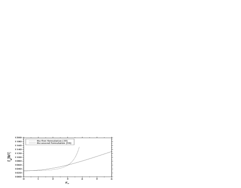
Figure 1: The total energy as a function of $g_{\omega}$ in the formalisms of Refs.Goeke and Alkofer . In the formalism of Ref.Goeke , the solution does not exist for $g_{\omega}\gtrsim 3.8$. $g_{\omega}\sim 4.6$ is predicted in the chiral perturbation analysis (see Sec.5).

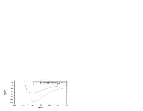
Figure 2: The binding energy in the formalisms of Refs.Goeke and Alkofer , where $g_{\omega}$=2.7 is used for the former and $g_{\omega}\sim 4.6$ for the latter.

In the second method, Eq. (26) is solved directly. Then the real and imaginary part of the one particle energy eigenvalue are derived as Alkofer .

$$\epsilon_{\mu}^{R} = \frac{1}{2}(\langle\Psi_{\mu}^{*}\mid H\mid\Psi_{\mu}\rangle+\langle\Psi_{\mu}\mid H\mid\Psi_{\mu}^{*}\rangle)$$

$$= \langle\Psi_{\mu}^{R}\mid H_{\Theta}\mid\Psi_{\mu}^{R}\rangle-\langle\Psi_{\mu}^{I}\mid H_{\Theta}\mid\Psi_{\mu}^{I}\rangle$$

$$- \langle\Psi_{\mu}^{I}\mid\omega\mid\Psi_{\mu}^{R}\rangle-\langle\Psi_{\mu}^{R}\mid\omega\mid\Psi_{\mu}^{I}\rangle,$$

$$\epsilon_{\mu}^{I} = \frac{1}{2}(\langle\Psi_{\mu}^{*}\mid H\mid\Psi_{\mu}\rangle-\langle\Psi_{\mu}\mid H\mid\Psi_{\mu}^{*}\rangle)$$ (34)

$$= \langle\Psi_{\mu}^{R}\mid\omega\mid\Psi_{\mu}^{R}\rangle-\langle\Psi_{\mu}^{I}\mid\omega\mid\Psi_{\mu}^{I}\rangle$$

$$+ \langle\Psi_{\mu}^{I}\mid H_{\Theta}\mid\Psi_{\mu}^{R}\rangle+\langle\Psi_{\mu}^{R}\mid H_{\Theta}\mid\Psi_{\mu}^{I}\rangle$$

where we employed the decomposition $\mid\Psi_{\mu}\rangle=\mid\Psi_{\mu}^{R}\rangle+i\mid\Psi_{\mu}^{I}\rangle$ and $\langle\Psi_{\mu}^{*}\mid=\langle\Psi_{\mu}^{R}\mid+i\langle\Psi_{\mu}^{I}\mid$. The valence quark energy is given by the same form as in the first method

$$E_{\rm val}^{R}=N_{c}\sum_{\nu}n_{\nu}|\epsilon_{\nu}^{R}|,\,E_{\rm val}^{I}=N_{c}\sum_{\nu}n_{\nu}{\rm sign}(\epsilon_{\nu}^{R})|\epsilon_{\nu}^{I}|.$$ (35)

The total energy in Euclidean space is

$$E_{\rm tot}[F,\omega,G]=E_{\rm val}^{R}+E_{\rm vac}^{R}+i(E_{\rm val}^{I}+E_{\rm vac}^{I})+E_{m}.$$ (36)

Thereby the total energy in Minkowski space is interpreted as

$$E_{\rm tot}[F,\omega,G]=E_{\rm val}^{R}+E_{\rm val}^{I}+E_{\rm vac}^{R}+E_{\rm vac}^{I}+E_{m}.$$ (37)

The equation of motion takes the form in (25) with the replacement of $\rho(\mbox{\boldmath$x$},\mbox{\boldmath$y$})$ and $\rho(\mbox{\boldmath$x$},\mbox{\boldmath$y$})$ by

$$\rho(\mbox{\boldmath$x$},\mbox{\boldmath$y$})=\rho_{R}^{\rm val}+\rho_{I}^{\rm val}+\rho_{R}^{\rm vac}+\rho_{i}^{\rm vac},$$ (38)

$$\rho_{R}^{\rm val}(\mbox{\boldmath$x$},\mbox{\boldmath$y$})+\rho_{R}^{\rm vac}(\mbox{\boldmath$x$},\mbox{\boldmath$y$})$$

$$~{}~{}=\sum_{\nu}\left[\psi_{\nu}^{R}(\mbox{\boldmath$x$})\bar{\psi}_{\nu}^{R}(\mbox{\boldmath$y$})-\psi_{\nu}^{I}(\mbox{\boldmath$x$})\bar{\psi}_{\nu}^{I}(\mbox{\boldmath$y$})\right](n_{\nu}+f_{\nu}^{R}),$$

$$\rho_{I}^{\rm val}(\mbox{\boldmath$x$},\mbox{\boldmath$y$})+\rho_{I}^{\rm vac}(\mbox{\boldmath$x$},\mbox{\boldmath$y$})$$

$$~{}~{}=\sum_{\nu}\left[\psi_{\nu}^{R}(\mbox{\boldmath$x$})\bar{\psi}_{\nu}^{I}(\mbox{\boldmath$y$})+\psi_{\nu}^{I}(\mbox{\boldmath$x$})\bar{\psi}_{\nu}^{R}(\mbox{\boldmath$y$})\right](n_{\nu}+f_{\nu}^{I}),$$

(39)

$$b(\mbox{\boldmath$x$},\mbox{\boldmath$y$})=b_{R}^{\rm val}+b_{I}^{\rm val}+b_{R}^{\rm vac}+b_{i}^{\rm vac},$$ (40)

$$b_{R}^{\rm val}(\mbox{\boldmath$x$},\mbox{\boldmath$y$})+b_{R}^{\rm vac}(\mbox{\boldmath$x$},\mbox{\boldmath$y$})$$

$$~{}~{}=\sum_{\nu}\left[\psi_{\nu}^{R}(\mbox{\boldmath$x$})\psi_{\nu}^{R\dagger}(\mbox{\boldmath$y$})-\psi_{\nu}^{I}(\mbox{\boldmath$x$})\psi_{\nu}^{I\dagger}(\mbox{\boldmath$y$})\right](n_{\nu}+f_{\nu}^{I}),$$

$$b_{I}^{\rm val}(\mbox{\boldmath$x$},\mbox{\boldmath$y$})+b_{I}^{\rm vac}(\mbox{\boldmath$x$},\mbox{\boldmath$y$})$$

$$~{}~{}=-\sum_{\nu}\left[\psi_{\nu}^{R}(\mbox{\boldmath$x$})\psi_{\nu}^{I\dagger}(\mbox{\boldmath$y$})+\psi_{\nu}^{I}(\mbox{\boldmath$x$})\bar{\psi}_{\nu}^{R\dagger}(\mbox{\boldmath$y$})\right](n_{\nu}+f_{\nu}^{R}),$$

(41)

where $f_{R}$ and $f_{I}$ are the imaginary part of the reguralized action written by

$$f_{\nu}^{R} = {\rm sign}(\epsilon_{\nu}^{R}){\mathcal{N}}_{\nu}+\frac{1}{\sqrt{\pi}}(\epsilon_{\nu}^{I}/\Lambda)\exp(-(\epsilon_{\nu}^{R}/\Lambda)^{2}),$$

$$f_{\nu}^{I} = {\rm sign}(\epsilon_{\nu}^{R}){\mathcal{N}}_{\nu}.$$

Figure 3: The profile functions of the chiral fields for $R$=0.75,1,1.5,2fm and the free ($R\to\infty$) solution.

IV The coupling constants of the vector mesons

In this section, we derive the coupling constants for the vector mesons. Expanding the real part of the effective action (8) up to second order in the heat-kernel expansion ebert86 , one obtains

$$S_{f}^{R(2)}=\frac{N_{c}}{16\pi^{2}}\int d^{4}x\Gamma\left(0,\left(\frac{M}{\Lambda}\right)^{2}\right)$$

$$\times{\rm tr}\left(M^{2}\partial_{\mu}U\partial^{\mu}U^{\dagger}+\frac{1}{3}F_{\mu\nu}^{k}F^{\mu\nu}_{k}+\frac{1}{3}F_{\mu\nu}^{0}F^{\mu\nu}_{0}\right),~{}~{}$$ (42)

where

$$F_{\mu\nu}^{k} = \partial_{\mu}V^{k}_{\nu}-\partial_{\nu}V^{k}_{\mu}+[V_{\mu}^{k},V_{\nu}^{k}],$$

$$F_{\mu\nu}^{0} = \partial_{\mu}V^{0}_{\nu}-\partial_{\nu}V^{0}_{\mu}+[V_{\mu}^{0},V_{\nu}^{0}].$$

We renormarize the vector meson fields $V_{\mu}^{k}=-ig_{\rho}\tilde{V}_{\mu}^{k},\ V_{\mu}^{0}=-ig_{\omega}\tilde{V}_{\mu}^{0}$ for later convenience. Then the total Lagrangian is given by

$$L^{R(2)} = \frac{N_{c}}{16\pi^{2}}\Gamma\left(0,\left(\frac{M}{\Lambda}\right)^{2}\right){\rm tr}\biggl{[}M^{2}\partial_{\mu}U\partial^{\mu}U^{\dagger}$$ (43)

$$+ \frac{g_{\rho}^{2}}{3}F_{\mu\nu}^{k}F^{\mu\nu}_{k}+\frac{g_{\omega}^{2}}{3}F_{\mu\nu}^{0}F^{\mu\nu}_{0}\biggl{]}$$

$$+ \frac{1}{2}\left(\frac{g_{\rho}^{2}}{4g_{1}}\right)(\tilde{V}^{k})^{2}+\frac{1}{2}\left(\frac{g_{\omega}^{2}}{4g_{2}}\right)(\tilde{V}^{0})^{2}$$

where

$$\tilde{F}_{\mu\nu}^{k} = \partial_{\mu}\tilde{V}^{k}_{\nu}-\partial_{\nu}\tilde{V}^{k}_{\mu}+g_{\rho}[\tilde{V}_{\mu}^{k},\tilde{V}_{\nu}^{k}],$$

$$\tilde{F}_{\mu\nu}^{0} = \partial_{\mu}\tilde{V}^{0}_{\nu}-\partial_{\nu}\tilde{V}^{0}_{\mu}+g_{\omega}[\tilde{V}_{\mu}^{0},\tilde{V}_{\nu}^{0}].$$ (44)

Comparing Eq. (43) with the massive Yang-Mills Lagrangian, the following relations for the parameters are obtained,

$$f_{\pi}^{2} = \frac{N_{c}M^{2}}{4\pi^{2}}\Gamma\left(0,\left(\frac{M}{\Lambda}\right)^{2}\right),$$ (45)

$$g_{\rho}^{2} = \frac{6M^{2}}{f_{\pi}^{2}},\ g_{\omega}^{2}=\frac{6M^{2}}{4f_{\pi}^{2}},$$ (46)

$$M_{\rho}^{2} = \frac{g_{\rho}^{2}}{4g_{1}},\ M_{\omega}^{2}=\frac{g_{\omega}^{2}}{4g_{2}}.$$ (47)

The experimental values are $f_{\pi}$=93MeV, $M$=350MeV, $M_{\rho}$=770MeV, $M_{\omega}$=783MeV, and hence

$$\Lambda=649{\rm MeV},~{}g_{1}=1.39,~{}g_{2}=0.34,$$

$$\hskip 28.45274ptg_{\rho}=9.22,~{}g_{\omega}=4.61.$$ (48)

As a reference, let us note that in Ref. saito94 ,

$$g_{\rho}=8.32\,,~{}g_{\omega}=4.41$$ (49)

are adopted for the MIT bag model.

Figure 4: The profile functions of $\rho$ meson for $R$=0.75,1,1.5,2fm and the free ($R\to\infty$) solution.

V The nuclear matter formulation

In this section we describe the numerical method of eigenproblem of the Hamiltonian (17). The Hamiltonian with hedgehog ansatz commutes with the parity and the grandspin operator given by

$$\bm{K}=\bm{j}+\bm{\tau}/2=\bm{l}+\bm{\sigma}/2+\bm{\tau}/2,$$

where $\bm{j},\bm{l}$ are respectively total angular momentum and orbital angular momentum. Accordingly, the angular basis can be written as

$$|(lj)KM\rangle=\sum_{j_{3}\tau_{3}}C^{KM}_{jj_{3}\frac{1}{2}\tau_{3}}\Bigl{(}\sum_{m\sigma_{3}}C^{jj_{3}}_{lm\frac{1}{2}\sigma_{3}}|lm\rangle|\frac{1}{2}\sigma_{3}\rangle\Bigr{)}|\frac{1}{2}\tau_{3}\rangle\,.$$

For $B=1$ solution, following states are possible

$$|0\rangle=|(K~{}K+\frac{1}{2})KM\rangle\,,$$

$$|1\rangle=|(K~{}K-\frac{1}{2})KM\rangle\,,$$

$$|2\rangle=|(K+1K+\frac{1}{2})KM\rangle\,,$$

$$|3\rangle=|(K-1K-\frac{1}{2})KM\rangle\,.$$

With this angular basis, the normalized eigenstates of the free Hamiltonian in a spherical box with radius $R$ can be constructed as follows:

$$u^{(a)}_{KM}=N_{k}\left(\begin{array}[]{c}i\omega^{+}_{\epsilon_{k}}j_{K}(kr)|0\rangle\\ \omega^{-}_{\epsilon_{k}}j_{K+1}(kr)|2\rangle\end{array}\right),$$ (53)

$$u^{(b)}_{KM}=N_{k}\left(\begin{array}[]{c}i\omega^{+}_{\epsilon_{k}}j_{K}(kr)|1\rangle\\ -\omega^{-}_{\epsilon_{k}}j_{K-1}(kr)|3\rangle\end{array}\right),$$ (56)

$$v^{(a)}_{KM}=N_{k}\left(\begin{array}[]{c}i\omega^{+}_{\epsilon_{k}}j_{K+1}(kr)|2\rangle\\ -\omega^{-}_{\epsilon_{k}}j_{K}(kr)|0\rangle\end{array}\right),$$ (59)

$$v^{(b)}_{KM}=N_{k}\left(\begin{array}[]{c}i\omega^{+}_{\epsilon_{k}}j_{K-1}(kr)|3\rangle\\ \omega^{-}_{\epsilon_{k}}j_{K}(kr)|1\rangle\end{array}\right),$$ (62)

with

$$N_{k}=\biggl{[}\frac{1}{2}R^{3}\Bigl{(}j_{K+1}(kR)\Bigr{)}^{2}\biggr{]}^{-1/2}$$ (63)

and $\omega^{+}_{\epsilon_{k}>0},\omega^{-}_{\epsilon_{k}<0}={\rm sgn}(\epsilon_{k}),\omega^{-}_{\epsilon_{k}>0},\omega^{+}_{\epsilon_{k}<0}=k/(\epsilon_{k}+M)$. The $u$ and $v$ correspond to the “natural” and “unnatural” components of the basis which stand for parity $(-1)^{K}$ and $(-1)^{K+1}$ respectively. The momenta are discretized by the boundary conditions $j_{K}(k_{i}R)=0$. The orthogonality of the basis is then satisfied by

$$\int^{R}_{0}drr^{2}j_{K}(k_{i}r)j_{K}(k_{j}r)$$

$$=\int^{R}_{0}drr^{2}j_{K\pm 1}(k_{i}r)j_{K\pm 1}(k_{j}r)$$

$$=\delta_{ij}\frac{R^{3}}{2}[j_{K\pm 1}(k_{i}R)]^{2}\,.$$ (64)

Figure 5: The profile functions of $\omega$ meson for $R$=0.75,1,1.5,2fm and the free ($R\to\infty$) solution.

Let us examine the boundary conditions for the Dirac and chiral fields to construct the nuclear matter solution in the Wigner-Seitz approximation. When the background chiral fields are periodic with lattice vector $\bm{a}$, the quark fields would be replaced by Bloch wave functions as $\psi(\bm{r}+\bm{a})=e^{i\bm{k}\cdot\bm{a}}\psi(\bm{r})$. In the Wigner-Seitz approximation, however, the soliton is put on the center of the spherical unit cell with the radius $R$ ($a=2R$) and the dispersion $\bm{k}$ is assumed to be zero. Then, $R$ is related to the baryon density through the relation

$$\rho_{\rm B}=\frac{3}{4\pi R^{3}}.$$ (65)

For the Dirac eigenstates, modification in the basis is needed. For odd number of $K$, the boundary condition is same as the free case with

$$j_{K}(k_{i}R)=0\,.$$ (66)

For even $K$, the following conditions must be satisfied

$$j_{K+1}(k^{(a)}_{i}R)=0,~{}~{}{\rm for}~{}~{}u^{(a)}_{KM},v^{(a)}_{KM}\,,$$

$$j_{K-1}(k^{(b)}_{i}R)=0,~{}~{}{\rm for}~{}~{}u^{(b)}_{KM},v^{(b)}_{KM}\,.$$ (67)

From the conditions (67) together with the equations of motion (25), we find the following boundary conditions for the profile function $F(r)$

$$\left.\begin{array}[]{c}~{}\sigma^{\prime}(0)=\sigma^{\prime}(R)=0\\ \pi(0)=\pi(R)=0\end{array}\right\}\Rightarrow F(0)=-\pi,F(R)=0\,,$$ (70)

which guarantees the periodicity and the unit topological charge inside the cell. Also, for vector meson profiles $\omega(r),G(r)$ we find the conditions instead of Eq.(16)

$$\omega^{\prime}(0) = 0,\,\,\omega^{\prime}(R)=0,$$ (71)

$$G(0) = 0,\,\,G(R)=0.$$ (72)

We solve (25) selfconsistently with boundary conditions (67)-(72) for varying $R$, from infinity (isolate the soliton) to origin (infinite density matter).

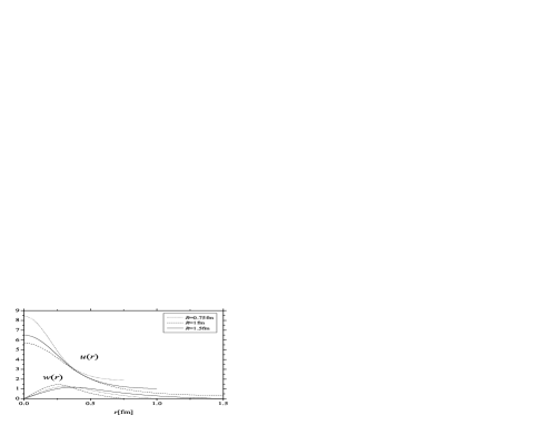
Figure 6: The “upper” $u(r)$ and the “lower” $w(r)$ positive component of valence quark wave functions for various cell radius $R$ with the boundary condition $w(R)=0$.

VI The numerical results

Since the equations of motion for mesons (25) and the Dirac equations for quarks (26) are highly non-linear, we solve these equations numerically by selfconsistent analysis. Using trial profiles for $\pi,\rho$ and $\omega$ mesons which satisfy the appropriate boundary conditions, we solve the Dirac equation (26). From Eq.(25), the profile functions $F(r)$, $G(r)$ and $\omega(r)$ are uniquely determined by using the eigenstates of Eq.(26). The new profiles produce new eigenstates. These procedures are repeated until selfconsistency is attained. We chose he quark mass $M=350$MeV which is mostly used and turned out to be the best choice for obtaining the various experimental observables christov96 ; alkofer96 . We performed the computation from $R$=5 (infinity) upto the value where the soliton solution breaks. The most dense solution is obtained for $R$=0.5fm which corresponds to the density $\rho$=1.91${\rm fm}^{-3}\sim 11\rho_{N}$. Note that $\rho_{N}$=0.17${\rm fm}^{-3}$ is the standard saturation density.

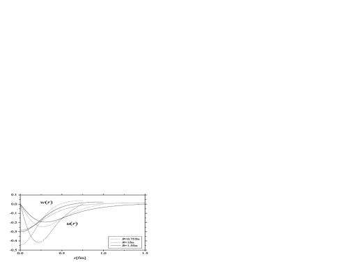
Figure 7: The negative component of valence quark wave functions. The label is as same as Fig. 6.

In Fig. 2, the binding energies computed in the two methods are shown. In the first method, the binding energy is too large, and the solutions disappear at relatively lower densities. Therefore, we focus our attention to the numerical results obtained in the second formalism hereafter.

Fig. 3 shows the self-consistent profile functions for free ($R\to\infty$) and for the various values of the cell radius $R$. Figs. 4, 5 show meson profile functions of $G(r),\omega(r)$ respectively. Fig. 6 shows the real part of the quark wave functions. Nonvanishing values of the upper component at the cell boundary $u(R)$ come from the zero-mode elements in the basis. The imaginary part of the quark wave functions derived in the second formulation is shown in Fig. 7.

In Fig. 8, we present the results of the total energy of the soliton as a function of $R$, for various values of the meson couplings. For only the pion coupling, the saturation can not be observed and the soliton disappears at very low density. Adding the $\rho$ meson, the soliton survives at higher density, but no saturation is observed. In the case of $\pi-\omega$, the total energy is enhanced and the soliton disappears at low density. The behavior is similar to the case of the pion coupling only. The saturation can be observed only when all the meson couplings are incorporated. The saturation point is at $R$=1.0fm corresponding to the density $\rho=0.24{\rm fm}^{-3}$ and the binding energy 53MeV. The density is very close to the experimental value for nuclear matter which is $R$=1.1fm corresponding to the density $\rho=0.17{\rm fm}^{-3}$. The binding energy is deeper compared to its empirical value, 16MeV. In Fig. 9 we show the binding energy for varying the constituent quark mass, which is the only free parameter in our model. The soliton survives for the constituent quark mass in the range 300MeV $\leq M\leq$ 440MeV. As $M$ increases, the saturation point moves to the lower density and the binding energy becomes shallower. For $M$=350MeV, the solution reaches to the highest density.

Let us estimate the nuclear incompressibility since it gives an important information for the saturation property of the matter. In Ref. barnea00 , the authors studied the soliton matter in the Friedberg-Lee model with quark-meson coupling using the Wigner-Seitz approximation. They estimated the incompressibility $K$ with the formula

$$K=R^{2}\frac{d^{2}E_{\rm B}}{dR^{2}}$$ (73)

and obtained $K\sim 1170$MeV. The experiment predicts $K$=100-500MeV and generally $K\sim 200$MeV. In our previous analysis nagai06 with only $\pi$ mesons, we obtained $K\sim 400$MeV. Our new result predicts $K\sim 270$MeV.

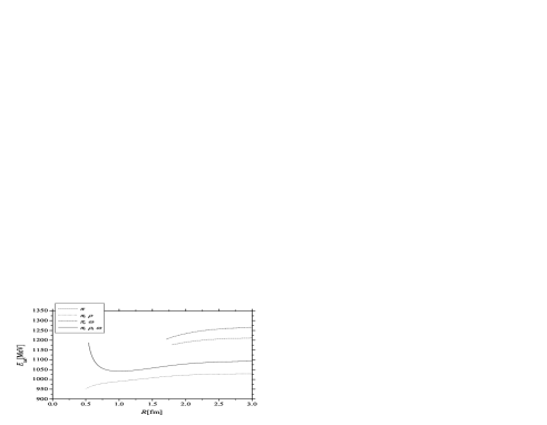
Figure 8: The total energy of soliton for the various combinations of the mesons.

VII Summary

In this paper we studied the nuclear matter solutions in the chiral quark soliton model. We adopted Wigner-Seitz approximation and investigated the saturation property of the matter solutions. To improve the qualitative behavior at the saturation point, we introduced the $\rho,\omega$ mesons in the model. The $\rho$ meson can be incorporated in a straightforward manner. On the other hand, Incorporating the $\omega$ meson makes the Hamiltonian complex-valued and requires some technique. We tested two distinct formulations proposed in Refs.Goeke ; Alkofer to solve the non-Hermitian eigenvalue problem. It turned out that the latter method produces the better behavior of solutions especially at high-density region. We performed the chiral perturbation analysis to determine the meson properties, i.e., the coupling constants and the cutoff parameter. We found that stable nuclear matter solutions exist when $\pi,\rho,\omega$ mesons are included with $330\leq M\leq 420$[MeV].

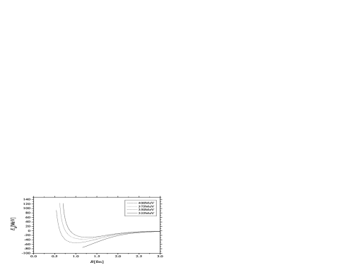
Figure 9: The total energy varying the constituent quark mass $M$.

From Fig. 8, one can speculate that the attractive property of the $\rho$ meson makes the total energy smaller and allows the solution to survive at the high density regime. The repulsive property of the $\omega$ meson makes the total energy larger and creates a short range (high density) core. Thus, the model having both effects can produce a stable nuclear matter.

Table 1: We present the $\rho$, $\omega$ coupling constant $g_{\rho}$, $g_{\omega}$, the total energy of the free nucleon $E_{\rm tot}^{\rm free}$ (its the experimental value is 939MeV), the binding energy $E_{\rm B}$ (16MeV), the saturation density $\rho_{s}$ (0.17${\rm fm}^{-3}$) and the incompressibility $K$ (210$\pm$30MeV) for the constituent quark mass $M$=350, 375, 400MeV.

$M[{\rm MeV}]$	$g_{\rho}$	$g_{\omega}$	$E_{\rm tot}^{\rm free}[{\rm MeV}]$	$E_{\rm B}[{\rm MeV}]$	$\rho_{s}[{\rm fm}^{-3}]$	$K$[MeV]
350	9.22	4.61	1095	53	0.24	271
375	9.88	4.94	1070	36	0.13	242
400	10.54	5.27	1044	29	0.11	274

Although our formulation realizes a improved nuclear saturation property, the binding energy is still large. Throughout the calculation, we set the constituent quark mass $M$=350MeV, in which the solution survives at highest density. By varying the value of $M$ in a few ten MeV, the saturation property should be improved (see Fig. 9). TABLE 1 shows the computed saturation properties for $M$=350, 375, 400MeV. $M$=375MeV seems to be the best choice, but the binding energy is still large. Another attempt to improve the binding energy may be to introduce heavier mesons, like axial vector meson $a_{1}$ ($\pi,\sigma,\rho,\omega$ and $a_{1}$ are the mesons which do not vanish for hedgehogs Goeke ). It is known that $a_{1}$ meson has attractive property like $\rho$ meson and then it would make the matter softer. Taking account the Fermi motion would also make the saturation energy shallower.

Acknowledgements

We are grateful to Kouichi Saito for fruitful discussions and comments.

References

• (1) Igor Klebanov, Nucl. Phys. B 262, 133 (1985).
• (2) E. Wüst, B. E. Brown and A. D. Jackson, Nucl. Phys. A 468, 450 (1987).
• (3) Alfred S. Goldhaber and N. S. Manton, Phys. Lett. B 19, 231 (1987).
• (4) L. Castillejo, P. S. Jones, A. D. Jackson, J. J. M. Verbaarschot and A. Jackson, Nucl. Phys. A 501, 450 (1987).
• (5) M. Kugler and S. Shtrikman, Phys. Rev. D 40, 3421 (1989).
• (6) Byung-Yoon Park, Dong-Pil Min, Mannque Rho and Vincente Vento, Nucl. Phys. A 707, 381 (2002).
• (7) Joachim Achtzehnter, Werner Scheid and Lawrence Wilets, Phys. Rev. D 32, 2414 (1985).
• (8) B. Banerjee, N. K. Glendenning and V. Soni, Phys. Lett. B 155, 213 (1985).
• (9) N. K. Glendenning and B. Banerjee, Phys. Rev. C 34, 1072 (1986).
• (10) Detlev Hahn and Norman K. Glendenning, Phys. Rev. C 36, 1181 (1987).
• (11) Urban Weber and Judith A. McGovern, Phys. Rev. C 57, 3376 (1998).
• (12) H. Reinhardt, B. V. Dang, and H. Schulz, Phys. Lett. B 159, 161 (1985).
• (13) M. C. Birse, J. J. Rehr and L. Wilets, Phys. Rev. C 38, 359 (1988).
• (14) Nir Barnea, Timothy S. Walhout, Nucl. Phys. A 677, 367 (2000).
• (15) M. Kutschera, C. J. Pethick and D. G. Ravenhall, Phys. Rev. Lett. 53, 1041 (1984).
• (16) D. I. Diakonov, V. Yu. Petrov, and P. V. Pobylitsa, Nucl. Phys. B 306, 809 (1988).
• (17) H. Reinhardt and R. Wünsch , Phys. Lett. B 215, 577 (1988).
• (18) Th. Meissner, F. Grümmer, and K. Goeke, Phys. Lett. B 227, 296 (1989).
• (19) M. Wakamatsu and H. Yoshiki, Nucl. Phys. A 524, 561 (1991).
• (20) Chr. V. Christov, A. Blotz, H.-C.Kim, P. Pobylitsa, T. Watabe, Th. Meissner, E. Ruiz Arriola, K. Goeke, Prog. Part. Nucl. Phys. 37, 91 (1996).
• (21) R. Alkofer, H. Reinhardt and H. Weigel, Phys. Rept. 265, 139 (1996)
• (22) P. Amore and A. De Pace, Phys. Rev. C 61, 055201 (2000).
• (23) I. Adjali, I. J. Aitchison, and J. A. Zuk, Nucl. Phys. A 537, 457 (1992).
• (24) S.Nagai, N.Sawado and N.Shiiki, Phys. Lett. B 632, 644 (2006).
• (25) C. Schüren, F. Döring, E. Ruiz Arriola, K. Goeke, Nucl. Phys. A 565, 687 (1993).
• (26) R. Alkofer, H. Reinhardt and H. Weigel, Nucl. Phys. A 570, 445 (1994)
• (27) S. Kahana and G. Ripka, Nucl. Phys. A 429, 462 (1984).
• (28) D. Ebert, H. Reinhardt, Nucl. Phys. B 271, 188 (1986).
• (29) K.Saito and A.W.Thomas, Phys. Lett. B 327, 9 (1994).