Ordinary muon capture on a proton in manifestly Lorentz invariant baryon chiral perturbation theory

Abstract

The amplitude for ordinary muon capture on the proton is evaluated, through the first four orders in the expansion parameter, in a manifestly Lorentz invariant form of baryon chiral perturbation theory. Expressions for the low energy constants in terms of physical quantities are obtained in each of the several renormalization schemes which have been proposed for forcing the relativistic approach to obey the same counting rules as obtained in heavy baryon chiral perturbation theory. The advantages and disadvantages of these schemes are discussed, using the muon capture results as an example, with the aim of gaining insight as to which scheme is preferable for practical calculations.

I Introduction

Ordinary, or non radiative, muon capture (OMC) has always been an interesting process because, unlike beta decay, there is a sufficiently high momentum transfer to explore weak-nucleon form factors away from $q^{2}=0$, where $q^{\mu}$ is the four momentum transfer between lepton and hadron currents. The induced pseudoscalar form factor, $G_{P}$, has been of particular interest and OMC is the main source of information on this form factor, see, e. g., Refs. Gorrev ; bem-jpg02 ; m-pr01 . Originally the amplitude for OMC was written down as the most general form of the current and OMC was simply an empirical way to determine the coefficients of this most general current. More recently it has become possible to calculate these form factors from a more fundamental point of view using an effective Lagrangian of chiral perturbation theory (ChPT) which incorporates the symmetries of QCD w-pa79 . Such calculations for OMC fear97 ; amk-prc01 ; bhm-npa01 or for the electromagnetic form factors of the nucleon bfhm-npa98 have been carried out in so called heavy baryon ChPT (HBChPT) which involves a Foldy-Wouthuysen-like expansion of the Lagrangian in powers of the inverse nucleon mass. A comprehensive, modern review with references to earlier work can be found in Srev .

The possibility of a fully relativistic ChPT approach to OMC, or any other process, has been elusive until recently. However there now have been several suggestions fuchs03 ; Sch04 ; BL ; et-prc98 ; geg03 for relativistic approaches footnote1 . The difficulty with relativistic theories has been the fact, as pointed out by Gasser, et al. Gasser , that they do not obey a counting procedure which would allow one to associate multiple loop diagrams with higher powers in an expansion in a small parameter. In fact in the relativistic approach these multiple loop diagrams, specifically those involving the relativistic nucleon propagator, can contribute to lower orders and so there is not a well defined prescription for deciding what diagrams to keep. One solution to this problem was the HBChPT approach in which diagrams involving more and more loops contribute at higher and higher orders in an expansion of the amplitude in powers of a typical momentum scale divided by the nucleon mass. While this approach works, it has the disadvantage of not being manifestly Lorentz invariant and of requiring increasingly complicated vertices as the order increases. The recent proposals for relativistic ChPT resolve this problem in a different way by showing that it is possible to define renormalization procedures for a manifestly Lorentz invariant theory which generate the same type of counting scheme which is present in HBChPT.

This paper thus has a number of aims. OMC is one of the simplest non trivial processes, and so we want to use it as laboratory to understand how the relativistic approach and the various renormalization schemes are applied to a practical case. We also want to compare and contrast the various proposed schemes to see if one is preferable for detailed calculations or if there are alternative methods which achieve the same result but which are easier to use.

We also want to obtain the muon capture amplitude and expressions for the low energy constants (LEC’s) in a unified and consistent approach. In the relativistic approach one can obtain these quantities to one higher order than is easily possible in HBChPT. This results from the fact that the Lagrangian, and the vertex operators originating from it, increases in complexity with increasing order much more rapidly for HBChPT than for the relativistic approach.

The OMC amplitude accesses the weak nucleon currents, vector and axial vector, the former being essentially the same as the electromagnetic current. There is enough information available to determine all of the LEC’s which appear. However, just as in HBChPT, the only unused information, once the LEC’s are determined, serves only to give the well known expression for $G_{P}$ in terms of the pion-nucleon coupling and the axial radius. Thus this evaluation of the OMC amplitude is mainly a way of determining the LEC’s and does not provide a ’new’ number for the rate.

Although many of the pieces have been obtained before in separate calculations, Gasser ; BLpiN ; fgs-jpg04 ; Fuchsthesis ; km-npa01 ; Schwthesis the results for the LEC’s depend on the details of the calculation and it becomes dangerous to lift these values for the LEC’s from disparate calculations and use them for other processes. Therefore it is important to have a consistent, consolidated and practical approach as this will provide the basis for determining the LEC’s which will be necessary for future calculations. Thus we see this calculation as a basis or starting point for planned similar consistent applications of this approach to processes such as $\pi p\rightarrow n\gamma$ where there are puzzles in the HBChPT approach arising from the appearance of unnaturally large LEC’s Fearpirad . It is also intended to be a starting point for a similar calculation of radiative muon capture, $\mu+p\rightarrow n+\nu+\gamma$, mmk-plb98 ; am-plb98 , where there are still unresolved problems relative to the extraction of $G_{P}$ Gorrev ; afm-prc01 ; tk-prc02 ; amk-prc02 .

II Weak form factors of the nucleon current

The S-matrix amplitude for the OMC process, $\mu+p\to n+\nu$, with momenta defined by $p_{\mu}+p_{i}=p_{f}+p_{\nu}$, is given in the notation of BjD by

$${\cal M}=\frac{-iG_{F}V_{ud}}{\sqrt{2}}\overline{u}(p_{\nu})\gamma_{\alpha}(1-\gamma_{5})u(p_{\mu})\overline{u}(p_{f})\tau_{-}\left[V^{\alpha}-A^{\alpha}\right]u(p_{i})$$ (1)

where the vector and axial vector nucleon current operators are given by

$$V^{\alpha} = G_{V}(q^{2})\gamma^{\alpha}+\frac{iG_{M}(q^{2})}{2m_{N}}\sigma^{\alpha\beta}q_{\beta}\,,$$

$$A^{\alpha} = G_{A}(q^{2})\gamma^{\alpha}\gamma_{5}+\frac{G_{P}(q^{2})}{m_{\mu}}q^{\alpha}\gamma_{5}\,.$$ (2)

Here $G_{F}$ is the Fermi constant as obtained from muon decay, $V_{ud}$ is an element of the CKM matrix, $m_{\mu}$ is the physical muon mass, $m_{N}$ is the average of physical neutron and proton masses, $m_{N}=(m_{n}+m_{p})/2$, and $\tau_{-}$ is the isospin lowering operator, $<n|\tau_{-}|p>=1$. Here we do not include radiative corrections aetal-plb04 and have neglected possible second class currents.

$G_{V}(q^{2})$, $G_{M}(q^{2})$, $G_{A}(q^{2})$ and $G_{P}(q^{2})$ are the weak form factors of interest, with the four momentum transfer $q^{\mu}=p_{f}^{\mu}-p_{i}^{\mu}$. The vector and weak magnetism form factors, $G_{V}$ and $G_{M}$ respectively, are related to the isovector electromagnetic form factors of the nucleon. The axial form factor at $q^{2}=0$, $G_{A}(0)$, is most accurately determined from neutron beta decay and $G_{P}$ is the induced pseudoscalar form factor which is accurately predicted by chiral symmetry. All of these form factors are functions of the four momentum transfer $q^{2}$ which for OMC on the proton is given by

$$q^{2}\rightarrow\frac{-m_{\mu}(m_{p}^{2}-m_{n}^{2}+m_{\mu}m_{p})}{m_{p}+m_{\mu}}=-0.88m_{\mu}^{2}.$$ (3)

Note that we have normalized these form factors using the physical masses $m_{\mu}$ and $m_{N}$ and that we have used the ChPT sign convention for $G_{A}$ and $G_{P}$, which makes them positive, in contrast to the convention which has been used historically and which is still used in the Particle Data Group listings PDG .

III Effective chiral Lagrangian

III.1 Effective Lagrangian

In the usual ChPT approach the effective Lagrangian is expanded in powers of a typical momentum - for this problem the muon mass $m_{\mu}$, the pion mass $m_{\pi}$, or the four momentum transfer squared $q^{2}$ - divided by a typical hadronic scale which we take as the physical nucleon mass. At each order the most general Lagrangian satisfying the symmetries of QCD is determined.

For this calculation we work in SU(2)$\times$SU(2) and use for the chiral Lagrangian ${\cal L}_{\chi}={\cal L}_{\pi N}+{\cal L}_{\pi}$ where ${\cal L}_{\pi N}$ and ${\cal L}_{\pi}$ are respectively the Lagrangians in the pion-nucleon and pion sectors. The pion-nucleon Lagrangian is expanded in terms of small quantities,

$${\cal L}_{\pi N}={\cal L}_{\pi N}^{(1)}+{\cal L}_{\pi N}^{(2)}+{\cal L}_{\pi N}^{(3)}+{\cal L}_{\pi N}^{(4)}+\cdots\,,$$ (4)

where the ellipsis represents the higher order terms and the superscript denotes the order of the Lagrangian.

The lowest order Lagrangian is given by the standard form

$${\cal L}_{\pi N}^{(1)}=\overline{\Psi}(i\not\!D-m+\frac{1}{2}g_{A}\not\!u\gamma_{5})\Psi\,.$$ (5)

Here the pion and nucleon fields are collected as

$$u^{2}=U=e^{i\vec{\tau}\cdot\vec{\pi}/F_{0}},\quad\quad\Psi=\left(\begin{array}[]{c}p\\ n\end{array}\right)\,.$$ (6)

The covariant derivative $D_{\mu}$, when acting on things transforming as nucleon fields, is defined as

$$D_{\mu}\Psi=(\partial_{\mu}+\Gamma_{\mu})\Psi\,,$$ (7)

with

$$\Gamma_{\mu}=\frac{1}{2}[u^{\dagger}(\partial_{\mu}-ir_{\mu})u+u(\partial_{\mu}-i\ell_{\mu})u^{\dagger}]$$ (8)

and with $\ell_{\mu}$ and $r_{\mu}$ constructed from the external vector and axial vector currents as $\ell_{\mu}=v_{\mu}-a_{\mu}$ and $r_{\mu}=v_{\mu}+a_{\mu}$. We also have

$$u_{\mu}=i[u^{\dagger}(\partial_{\mu}-ir_{\mu})u-u(\partial_{\mu}-i\ell_{\mu})u^{\dagger}]\,.$$ (9)

The parameters appearing in this lowest order Lagrangian, $m,F_{0},g_{A}$ are respectively the ’bare’ or unrenormalized values of the nucleon mass, the pion decay coupling and $G_{A}(0)$ and the fields are the ’bare’ fields.

The higher order Lagrangians are given by

$${\cal L}_{\pi N}^{(2)}=\sum_{i=1}^{7}c_{i}\overline{\Psi}{\cal O}_{i}\Psi\,,\ \ \ {\cal L}_{\pi N}^{(3)}=\sum_{i=1}^{23}d_{i}\overline{\Psi}{\cal O}_{i}\Psi\,,\ \ \ {\cal L}_{\pi N}^{(4)}=\sum_{i=1}^{118}e_{i}\overline{\Psi}{\cal O}_{i}\Psi\,,$$ (10)

where the $c_{i},d_{i},e_{i}$ are the LEC’s and where the basis functions ${\cal O}_{i}$ are given in Ref. Fettes00 Tables III, IV and V. Note however that we always normalize the LEC’s to the physical mass $m_{N}$ rather than to $m$.

We will also need the Lagrangian in the purely meson sector, as the results depend on that choice as well. We will take the standard one

$${\cal L}_{\pi}={\cal L}_{\pi}^{(2)}+{\cal L}_{\pi}^{(4)}+\cdots\,,$$ (11)

where the lowest order Lagrangian is given by

$${\cal L}_{\pi}^{(2)}=\frac{F_{0}^{2}}{4}<D_{\mu}U(D^{\mu}U)^{\dagger}>+\frac{F_{0}^{2}}{4}<\chi U^{\dagger}+U\chi^{\dagger}>.$$ (12)

Here the covariant derivative acting on quantities transforming as $U$ is given by

$$D_{\mu}U=\partial_{\mu}U-ir_{\mu}U+iU\ell_{\mu}\,.$$ (13)

We also have

$$\chi=2B_{0}(s+ip)\,,$$ (14)

where $s$ and $p$ are the external scalar and pseudoscalar current and the chiral symmetry breaking is introduced as usual by taking $p=0$ and $s=\hat{m}$ with $\hat{m}=(m_{u}+m_{d})/2$ the average of up and down quark masses. The parameter $B_{0}$ is given in terms of the lowest order pion mass $m_{0\pi}$ (cf. Eq. (140)) by $2B_{0}\hat{m}=m_{0\pi}^{2}$. For the fourth order Lagrangian we take the Gasser-Sainio-Švarc Gasser form of the Gasser-Leutwyler Lagrangian GL given explicitly for example by Eq. (D.13) of Ref. Srev .

III.2 Counting rules and ’non counting’ terms from loop diagrams

In the usual HBChPT approach the Lagrangians ${\cal L}_{\pi N}^{(1)},{\cal L}_{\pi N}^{(2)},{\cal L}_{\pi N}^{(3)},{\cal L}_{\pi N}^{(4)}$, or more precisely the HBChPT expansions of these Lagrangians, contribute tree level diagrams respectively of order $p,p^{2},p^{3},p^{4}$ where we mean by $p$ the generic small expansion parameter, e.g., $m_{\pi}/m_{N}$. As a consequence of using the dimensional regularization procedure for regularizing the integrals, Djuk05 the one loop graphs containing only vertices from ${\cal L}_{\pi N}^{(1)}$ contribute at ${\cal O}(p^{3})$ and those containing one vertex from ${\cal L}_{\pi N}^{(2)}$ contribute at ${\cal O}(p^{4})$. Two or more loop graphs contribute only at ${\cal O}(p^{5})$ or higher.

In the relativistic approach however the counting breaks down, with multi-loop graphs contributing to lower orders, ${\cal O}(p^{2})$, ${\cal O}(p^{3})$, etc. Gasser , than that obtained in HBChPT. Thus one needs to develop some different scheme for ordering the various contributions and determining which to keep.

From a purely practical point of view it is rarely possible, or necessary, to consider more than one loop. Furthermore one of the most important general results of Becher and Leutwyler BL or more particularly Fuchs, et al. fuchs03 is that it is always possible to absorb into the LEC’s those terms from multi-loop diagrams which do not obey the HBChPT counting rules. Thus we will here consider only one loop diagrams and assume that all contributions from multi-loop diagrams are either ${\cal O}(p^{5})$ or, in accord with the general result, have been absorbed in the LEC’s in the original Lagrangians as defined in Eqs. (5) and (10).

We note also, as will be seen from the explicit expressions below, that associated with each loop is the factor $1/(4\pi F_{0})^{2}$. By neglecting multi-loop diagrams we are neglecting terms containing higher powers of this factor, e.g. $1/(4\pi F_{0})^{4}$. Such higher powers will also arise from the expansion of unrenormalized quantities in one loop diagrams about renormalized values. We will always drop such higher powers of $1/(4\pi F_{0})^{2}$, arguing that such approximation is consistent with our neglect of multi-loop diagrams.

Thus to summarize, we will work consistently to one loop, and to ${\cal O}(p^{4})$. This means that we will keep all terms of ${\cal O}(p^{4})$ or lower except for those originating in multi-loop diagrams, which we assume to have been absorbed in the LEC’s. We also drop terms involving $1/(4\pi F_{0})$ to the fourth or higher power, an approximation which is consistent with the neglect of multi-loop contributions, which have these same factors. Note also that those one loop diagrams which have higher order Lagrangians at the vertices and thus which are of ${\cal O}(p^{5})$ or higher in the HBChPT sense will also be dropped, again assuming that any lower order terms from these diagrams which do not obey this counting have been absorbed in the LEC’s.

This choice of diagrams and terms to keep is to some extent dictated by the practicalities of doing such calculations. Two loop diagrams and those with many higher order vertices are difficult to handle, and normally would be considered only if there were some special circumstance which suggests that they would be large. Perhaps the most important result arising from the work of Refs. BL ; fuchs03 is that this is a consistent procedure, i.e. that lower order contributions which originate in these higher order diagrams which we must neglect can in fact be absorbed in the LEC’s in a way that preserves the usual HBChPT counting procedures.

In the relativistic approach there will also be terms, a finite number of them, coming from the one loop diagrams we keep, which do not obey HBChPT counting, e.g. those of ${\cal O}(p^{2})$. We will flag these terms, but for now keep all of them explicitly, until we discuss the various renormalization schemes which have been proposed, as these schemes differ primarily in how they treat these ’non counting’ terms.

IV Evaluation of the NN 3-point vertex : vector and axial vector currents

IV.1 Preliminaries

We now proceed to evaluate the amplitude of Eq. (1). The amplitude originates in the usual current-current interaction which couples the lepton current to the weak nucleon current. The lepton current is given by the relativistic tree-level current, $l_{\alpha}=\bar{u}_{\nu}\gamma_{\alpha}(1-\gamma_{5})u_{\mu}$. The $(V-A)$ weak nucleon current is calculated from the effective Lagrangian using the approach described above.

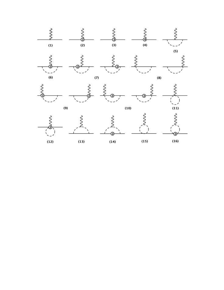
Figure 1: Diagrams which contribute to the coupling of external vector and axial vector currents to the nucleon. The solid, dashed, and wiggly lines correspond respectively to nucleons, pions, and external vector or axial vector fields. The unlabeled vertices come from ${\cal L}_{\pi N}^{(1)}$ whereas the ones labeled 2,3,4 come respectively from ${\cal L}_{\pi N}^{(2)}$, ${\cal L}_{\pi N}^{(3)}$ and ${\cal L}_{\pi N}^{(4)}$.

There are three contributions to the weak-nucleon-nucleon vertex. The first two of these involve coupling of the nucleons to an external vector field and to an external axial field. The diagrams which contribute to these two contributions are given in Fig. 1. The third contribution, to be discussed in the next section, involves coupling to the pion, which by virtue of its coupling to the leptonic current contributes to the overall axial weak nucleon current.

We take for the external vector current $v_{\mu}\rightarrow v_{\mu}^{(s)}+\vec{\tau}\cdot\vec{v}_{\mu}$, i.e., we divide the current into isoscalar and isovector part. Only the isovector part contributes to the weak current, but we will keep both for completeness, and to allow evaluation of some of the LEC’s via a connection to the isoscalar electromagnetic form factors of the nucleon. Similarly we take $a_{\mu}\rightarrow a_{\mu}^{(s)}+\vec{\tau}\cdot\vec{a}_{\mu}$, but in this case will drop the isoscalar axial current $a_{\mu}^{(s)}$.

IV.2 Tree level diagrams

The tree level contributions to the amplitude correspond to diagrams 1-4 in Fig. 1 and are given by

$$M_{1V} = i\sqrt{Z_{N}}\overline{\Psi}_{f}(v_{\mu}^{(s)}+\vec{\tau}\cdot\vec{v}_{\mu})\gamma^{\mu}\Psi_{i}\sqrt{Z_{N}}\,,$$ (15)

$$M_{1A} = ig_{A}\sqrt{Z_{N}}\overline{\Psi}_{f}\vec{\tau}\cdot\vec{a}_{\mu}\gamma^{\mu}\gamma_{5}\Psi_{i}\sqrt{Z_{N}}\,,$$ (16)

$$M_{2V} = i\sqrt{Z_{N}}\overline{\Psi}_{f}\frac{i\sigma^{\mu\nu}q_{\nu}}{2m_{N}}[(c_{6}+2c_{7})v_{\mu}^{(s)}+c_{6}\vec{\tau}\cdot\vec{v}_{\mu}]\Psi_{i}\sqrt{Z_{N}}\,,$$ (17)

$$M_{2A} = 0\,,$$ (18)

$$M_{3V} = i\overline{\Psi}_{f}(q^{\mu}q^{\nu}-q^{2}g^{\mu\nu})(p_{i}+p_{f})_{\nu}(\frac{2d_{7}}{m_{N}}v_{\mu}^{(s)}+\frac{d_{6}}{m_{N}}\vec{\tau}\cdot\vec{v}_{\mu})\Psi_{i}\,,$$ (19)

$$M_{3A} = i\overline{\Psi}_{f}\gamma^{\mu}\gamma_{5}[4m_{0\pi}^{2}d_{16}\vec{\tau}\cdot\vec{a}_{\mu}+d_{22}(q^{2}g_{\mu\nu}-q_{\mu}q_{\nu})\vec{\tau}\cdot\vec{a}^{\nu}]\Psi_{i}\,,$$ (20)

$$M_{4V} = i\overline{\Psi}_{f}i\sigma^{\mu\nu}q_{\nu}[4(q^{2}e_{54}-4m_{0\pi}^{2}e_{105})v_{\mu}^{(s)}+2(q^{2}e_{74}-4m_{0\pi}^{2}e_{106})\vec{\tau}\cdot\vec{v}_{\mu}]\Psi_{i}\,,$$ (21)

$$M_{4A} = 0\,.$$ (22)

Here the subscript $V$ or $A$ refers to coupling to vector or axial current respectively and the number refers to the particular diagram in Fig. 1. For these and subsequent amplitude expressions $\overline{\Psi}_{f}$ and $\Psi_{i}$ are to be interpreted as wave functions, rather than the fields of the original Lagrangian. That is, they are still two component objects in isospin space, but made up of spinors $\overline{u}(p_{f})$ and $u(p_{i})$ rather than fields. In the HBChPT counting system these tree level diagrams contribute to ${\cal O}(p)$, ${\cal O}(p^{2})$, ${\cal O}(p^{3})$,${\cal O}(p^{4})$ respectively. Note that the nucleon wave function renormalization factor $Z_{N}$ appears only in the $M_{1}$ and $M_{2}$ amplitudes which is a consequence of the fact, as shown in Eq. (160) of Appendix B, that the leading corrections to $Z_{N}$ are two orders higher, $Z_{N}=1+{\cal O}(p^{2})$.

IV.3 Leading one loop diagrams

The next set of diagrams consists of those one loop diagrams with all vertices coming from ${\cal L}_{\pi N}^{(1)}$. In the HBChPT sense these all contribute first at ${\cal O}(p^{3})$ , but in the relativistic approach they will also contribute some ’non counting’ terms of ${\cal O}(p^{2})$ as well as relativistic corrections of ${\cal O}(p^{4})$ and higher.

We express these amplitudes in terms of a general loop integral $I_{\pi\pi....NN....}$ which is defined in detail in Appendix A. For present purposes it is sufficient to note that $I_{\pi\pi....NN....}[k_{i},....p_{j},...,A]$ refers to a loop integral which contains a pion propagator for each subscript $\pi$ with momenta of the form $k_{i}+\ell$ and a nucleon propagator denominator for each subscript $N$ with momenta of the form $p_{j}+\ell$. The loop integration variable $\ell$ footnote2 is chosen so that the first pion momentum $k_{1}$ is zero and that argument is normally not put in explicitly. $A$ is whatever is in the numerator.

In terms of these loop integrals the lowest order one loop amplitudes are given by

$$M_{5V} = \frac{ig_{A}^{2}}{4F_{0}^{2}}\overline{\Psi}_{f}(3v_{\mu}^{(s)}-\vec{\tau}\cdot\vec{v}_{\mu})I_{\pi NN}[p_{i},p_{f},\not\!\ell\gamma_{5}(\not\!p_{f}+\not\!\ell+m)\gamma^{\mu}(\not\!p_{i}+\not\!\ell+m)\not\!\ell\gamma_{5}]\Psi_{i}\,,$$ (23)

$$M_{5A} = -\frac{ig_{A}^{3}}{4F_{0}^{2}}\overline{\Psi}_{f}\vec{\tau}\cdot\vec{a}_{\mu}I_{\pi NN}[p_{i},p_{f},\not\!\ell\gamma_{5}(\not\!p_{f}+\not\!\ell+m)\gamma^{\mu}\gamma_{5}(\not\!p_{i}+\not\!\ell+m)\not\!\ell\gamma_{5}]\Psi_{i}\,,$$ (24)

$$M_{8V} = \frac{ig_{A}^{2}}{F_{0}^{2}}\overline{\Psi}_{f}\vec{\tau}\cdot\vec{v}_{\mu}\{I_{\pi N}[p_{f},\not\!\ell\gamma_{5}(\not\!p_{f}+\not\!\ell+m)\gamma^{\mu}\gamma_{5}]$$ (25)

$$\quad\quad\quad+I_{\pi N}[p_{i},\gamma^{\mu}\gamma_{5}(\not\!p_{i}+\not\!\ell+m)\not\!\ell\gamma_{5}]\}\Psi_{i}\,,$$

$$M_{8A} = \frac{ig_{A}}{F_{0}^{2}}\overline{\Psi}_{f}\vec{\tau}\cdot\vec{a}_{\mu}\{I_{\pi N}[p_{f},\not\!\ell\gamma_{5}(\not\!p_{f}+\not\!\ell+m)\gamma^{\mu}]+I_{\pi N}[p_{i},\gamma^{\mu}(\not\!p_{i}+\not\!\ell+m)\not\!\ell\gamma_{5}]\}\Psi_{i}\,,$$ (26)

$$M_{11V} = -\frac{i}{F_{0}^{2}}\overline{\Psi}_{f}\vec{\tau}\cdot\vec{v}_{\mu}\gamma^{\mu}\Psi_{i}I_{\pi}[1]\,,$$ (27)

$$M_{11A} = -\frac{ig_{A}}{F_{0}^{2}}\overline{\Psi}_{f}\vec{\tau}\cdot\vec{a}_{\mu}\gamma^{\mu}\gamma_{5}\Psi_{i}I_{\pi}[1]\,,$$ (28)

$$M_{13V} = -\frac{ig_{A}^{2}}{F_{0}^{2}}\overline{\Psi}_{f}\vec{\tau}\cdot\vec{v}_{\mu}I_{\pi\pi N}[-q,p_{i},(2\ell-q)^{\mu}(\not\!\ell-\not\!q)\gamma_{5}(\not\!p_{i}+\not\!\ell+m)\not\!\ell\gamma_{5}]\Psi_{i}\,,$$ (29)

$$M_{13A} = 0\,,$$ (30)

$$M_{15V} = \frac{i}{2F_{0}^{2}}\overline{\Psi}_{f}\vec{\tau}\cdot\vec{v}_{\mu}I_{\pi\pi}[-q,(2\ell-q)^{\mu}(2\not\!\ell-\not\!q)]\Psi_{i}\,,$$ (31)

$$M_{15A} = 0\,.$$ (32)

IV.4 Further one loop diagrams

The next class of one loop diagrams consists of those with one vertex from ${\cal L}_{\pi N}^{(2)}$ with all others from ${\cal L}_{\pi N}^{(1)}$. In the HBChPT sense these would be of ${\cal O}(p^{4})$, but again in the relativistic formulation they will have ’non counting’ terms of lower order.

These amplitudes are given by

$$M_{6V} = \frac{ig_{A}^{2}}{4F_{0}^{2}}\overline{\Psi}_{f}[3(c_{6}+2c_{7})v_{\mu}^{(s)}-c_{6}\vec{\tau}\cdot\vec{v}_{\mu}]$$ (33)

$$\quad\quad\quad\times I_{\pi NN}[p_{i},p_{f},\not\!\ell\gamma_{5}(\not\!p_{f}+\not\!\ell+m)\frac{i\sigma^{\mu\nu}q_{\nu}}{2m_{N}}(\not\!p_{i}+\not\!\ell+m)\not\!\ell\gamma_{5}]\Psi_{i}\,,$$

$$M_{6A} = 0\,,$$ (34)

$$M_{9V} = 0\,,$$ (35)

$$M_{9A} = -\frac{ig_{A}}{4F_{0}^{2}}\overline{\Psi}_{f}\vec{\tau}\cdot\vec{a}_{\mu}\left\{I_{\pi N}[p_{f},\not\!\ell\gamma_{5}(\not\!p_{f}+\not\!\ell+m)[\frac{4c_{2}}{m_{N}^{2}}(p_{i}^{\mu}p_{i}\cdot\ell+(p_{f}+\ell)^{\mu}(p_{f}+\ell)\cdot\ell)\right.$$ (36)

$$+ \left.8c_{3}\ell^{\mu}-2i\sigma^{\mu\nu}(4c_{4}\ell_{\nu}+\frac{c_{6}}{m_{N}}q_{\nu})]]\right.$$

$$+ \left.I_{\pi N}[p_{i},[\frac{4c_{2}}{m_{N}^{2}}(p_{f}^{\mu}p_{f}\cdot\ell+(p_{i}+\ell)^{\mu}(p_{i}+\ell)\cdot\ell)+8c_{3}\ell^{\mu}\right.$$

$$+ \left.2i\sigma^{\mu\nu}(4c_{4}\ell_{\nu}-\frac{c_{6}}{m_{N}}q_{\nu})](\not\!p_{i}+\not\!\ell+m)\not\!\ell\gamma_{5}]\right\}\Psi_{i}\,,$$

$$M_{12V} = \frac{3ic_{2}}{F_{0}^{2}m_{N}^{2}}\overline{\Psi}_{f}(v_{\mu}^{(s)}+\vec{\tau}\cdot\vec{v}_{\mu})(p_{i}+p_{f})_{\nu}I_{\pi}[\ell^{\mu}\ell^{\nu}]\Psi_{i}+\frac{c_{6}}{2F_{0}^{2}m_{N}}\overline{\Psi}_{f}\sigma^{\mu\nu}q_{\nu}\vec{\tau}\cdot\vec{v}_{\mu}\Psi_{i}I_{\pi}[1]\,,$$ (37)

$$M_{12A} = 0\,,$$ (38)

$$M_{16V} = -\frac{2c_{4}}{F_{0}^{2}}\overline{\Psi}_{f}\sigma^{\mu\nu}q_{\nu}\vec{\tau}\cdot\vec{v}_{\alpha}I_{\pi\pi}[-q,(2\ell-q)^{\alpha}\ell_{\mu}]\Psi_{i}\,,$$ (39)

$$M_{16A} = 0\,.$$ (40)

IV.5 Mass insertion terms

The final set of amplitudes arises from the mass insertions on internal nucleon lines. These insertions come from the NN two point term in ${\cal L}_{\pi N}^{(2)}$, namely $\overline{\Psi}_{f}4c_{1}m_{0\pi}^{2}\Psi_{i}$. The relevant amplitudes, those for diagrams 7,10,14 of Fig. 1, can be obtained from the underlying diagrams 5,8,13 respectively by the substitution for each nucleon propagator in turn

$$\frac{i}{\not\!p-m+i\epsilon}\rightarrow\frac{i}{\not\!p-m+i\epsilon}(4ic_{1}m_{0\pi}^{2})\frac{i}{\not\!p-m+i\epsilon}.$$ (41)

An alternative procedure is to observe that $m$ appears in the loop integrals only in the propagators, since we normalized all the constants in the Lagrangian to $m_{N}$ not $m$. Thus we can use the fact that

$$i(4ic_{1}m_{0\pi}^{2})\frac{\partial}{\partial m}(\frac{i}{\not\!p-m+i\epsilon})=\frac{i}{\not\!p-m+i\epsilon}(4ic_{1}m_{0\pi}^{2})\frac{i}{\not\!p-m+i\epsilon}.$$ (42)

This allows us to obtain the amplitudes with mass insertions by taking derivatives of the corresponding amplitudes without insertions. As detailed in Appendix A this approach, while exact, may not be as useful as one might expect because the derivative in effect reduces the power of small expansion parameter. Thus in some cases one has to expand the initial integral to higher order than needed for it alone so as to get the mass insertion diagrams to the appropriate order. We actually calculated these mass insertion diagrams explicitly and used this derivative procedure to check the results.

Another approach is to observe that (see Appendix B) the ’bare’ nucleon mass which appears in the original Lagrangian is related to the physical mass by the relation

$$m_{N}=m-4c_{1}m_{0\pi}^{2}+{\cal O}(p^{4}).$$ (43)

Thus a propagator with mass $m\rightarrow m_{N}$ can be expanded as

$$\frac{i}{\not\!p-m_{N}+i\epsilon}\rightarrow\frac{i}{\not\!p-m+i\epsilon}+\frac{i}{\not\!p-m+i\epsilon}(4ic_{1}m_{0\pi}^{2})\frac{i}{\not\!p-m+i\epsilon}+...\,.$$ (44)

Thus if we replace $m\rightarrow m_{N}$ in the propagators in the one loop diagrams we effectively include the mass insertion diagrams 7,10,14 of Fig. 1. At the same time we reduce the number of separate diagrams to be calculated and reduce by one the maximum number of propagators involved in the loop integrals which must be calculated. Both of these offer significant calculational advantages. However this expansion only works to first order, so one must keep only terms in the expansion of the propagators which are linear in $c_{1}$. This requires extreme care since $c_{1}$ appears also in other places in the amplitudes so that in general there are legitimate terms involving $c_{1}^{2}$ which must be kept.

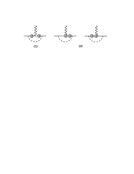
Figure 2: Diagrams which are higher order and which would not be included in an explicit calculation. However parts of these diagrams would be included implicitly by using the physical mass $m_{N}$ in the propagators of loop integrals.

Note that simply replacing $m\rightarrow m_{N}$ in all the propagators is not exactly equivalent to the direct calculation of the mass insertion diagrams. The expansion of Eq. (44) only works to lowest order, so with such a substitution there will be some spurious higher order terms implicitly included. Also implicitly included will be diagrams like those of Fig. 2 which involve two mass insertions or which involve one mass insertion plus a vertex from ${\cal L}_{\pi N}^{(2)}$. These would not have been included in a direct calculation of the mass insertion diagrams as they would have been nominally of too high order. To the order we are considering most of these extra terms can be neglected. In fact in HBChPT all would be of higher order. However in the relativistic approach there will be a few terms arising from the ’non counting’ terms from diagrams such as those of Fig. 2 which will appear in the amplitude in this approximation and not in the explicit calculation.

To repeat, our approach was to calculate the mass insertion diagrams explicitly and thus our results may differ from calculations which use one of the above approximations.

IV.6 Summary

By summing all of the amplitudes given above we obtain the complete weak nucleon-nucleon amplitude arising from interaction with external vector and axial vector fields.

V Evaluation of the NN 3-point vertex : pion terms

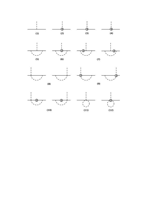
Figure 3: Diagrams which contribute to the $\pi$NN vertex.

The third contribution which must be evaluated comes from the pion-nucleon-nucleon vertex and will contribute to the axial current. The diagrams which are needed are given in Fig. 3 and the amplitudes associated with those diagrams are given by

$$M_{1\pi} = -\frac{g_{A}}{2F_{0}}\sqrt{Z_{N}}\overline{\Psi}_{f}\vec{\tau}\cdot\vec{\pi}\not\!q\gamma_{5}\Psi_{i}\sqrt{Z_{N}}\sqrt{Z_{\pi}}\,,$$ (45)

$$M_{2\pi} = 0\,,$$ (46)

$$M_{3\pi} = \frac{m_{0\pi}^{2}}{F_{0}}(d_{18}-2d_{16})\overline{\Psi}_{f}\vec{\tau}\cdot\vec{\pi}\not\!q\gamma_{5}\Psi_{i}\,,$$ (47)

$$M_{4\pi} = 0\,,$$ (48)

$$M_{5\pi} = \frac{g_{A}^{3}}{8F_{0}^{3}}\overline{\Psi}_{f}\vec{\tau}\cdot\vec{\pi}I_{\pi NN}[p_{i},p_{f},\not\!\ell\gamma_{5}(\not\!p_{f}+\not\!\ell+m)\not\!q\gamma_{5}(\not\!p_{i}+\not\!\ell+m)\not\!\ell\gamma_{5}]\Psi_{i}\,,$$ (49)

$$M_{6\pi} = 0\,,$$ (50)

$$M_{8\pi} = -\frac{g_{A}}{4F_{0}^{3}}\overline{\Psi}_{f}\vec{\tau}\cdot\vec{\pi}\left\{I_{\pi N}[p_{f},\not\!\ell\gamma_{5}(\not\!p_{f}+\not\!\ell+m)(\not\!q-\not\!\ell)]\right.$$ (51)

$$+\left.I_{\pi N}[p_{i},(\not\!q+\not\!\ell)(\not\!p_{i}+\not\!\ell+m)\not\!\ell\gamma_{5}]\right\}\Psi_{i}\,,$$

$$M_{9\pi} = -\frac{g_{A}}{2F_{0}^{3}}\overline{\Psi}_{f}\vec{\tau}\cdot\vec{\pi}\{I_{\pi N}[p_{f},\not\!\ell\gamma_{5}(\not\!p_{f}+\not\!\ell+m)[-4c_{1}m_{0\pi}^{2}$$ (52)

$$-\frac{c_{2}}{m_{N}^{2}}((p_{f}+\ell)\cdot\ell(p_{f}+\ell)\cdot q+p_{i}\cdot\ell p_{i}\cdot q)-2c_{3}\ell\cdot q-2ic_{4}\sigma^{\mu\nu}\ell_{\mu}q_{\nu}]]$$

$$-I_{\pi N}[p_{i},[-4c_{1}m_{0\pi}^{2}+\frac{c_{2}}{m_{N}^{2}}((p_{i}+\ell)\cdot\ell(p_{i}+\ell)\cdot q+p_{f}\cdot\ell p_{f}\cdot q)+2c_{3}\ell\cdot q$$

$$-2ic_{4}\sigma^{\mu\nu}\ell_{\mu}q_{\nu}](\not\!p_{i}+\not\!\ell+m)\not\!\ell\gamma_{5}]\}\Psi_{i}\,,$$

$$M_{11\pi} = \frac{g_{A}}{6F_{0}^{3}}\overline{\Psi}_{f}\vec{\tau}\cdot\vec{\pi}\not\!q\gamma_{5}\Psi_{i}I_{\pi}[1]\,,$$ (53)

$$M_{12\pi} = 0\,.$$ (54)

Again the mass insertion diagrams 7 and 10 are obtained by making the replacement of Eq. (41) in diagrams 5 and 8.

To get the contribution to the weak nucleon-nucleon axial current from this $\pi NN$ amplitude we make the replacement (for $q^{2}\neq m_{\pi}^{2}$) $\vec{\tau}\cdot\vec{\pi}\rightarrow 2iF_{\pi}q^{\mu}\vec{\tau}\cdot\vec{a}_{\mu}/(q^{2}-m_{\pi}^{2})$. This arises from the addition of a pion propagator and pion decay vertex to the $\pi NN$ vertex. Note that the parameters $F_{\pi}$ and $m_{\pi}$ are the physical ones. Since we have associated a $\sqrt{Z_{\pi}}$ with the amplitude $M_{1\pi}$ so that it is renormalized, we need to use here the renormalized propagator and renormalized pion decay vertex to make the overall amplitude renormalized.

VI Evaluation, regularization and renormalization

The first step in evaluating these amplitudes is to reduce the numerators of the loop integrals. This is done using the standard algebra of Dirac matrices and the usual tensor decomposition of integrals with $\ell^{\mu},\ell^{\mu}\ell^{\nu},...$ in the numerator. The end result is that the full amplitude can be expressed in terms of the following loop integrals with unit numerator: $I_{\pi}[1],I_{\pi N}[p,1],I_{NN}[p_{i},p_{f},1],I_{\pi\pi}[q,1],I_{\pi NN}[p_{i},p_{f},1],I_{\pi\pi N}[-q,p,1]$, where $p$ can be $p_{i}$ or $p_{f}$. For the diagrams with the mass insertion put in explicitly we need the additional integrals $I_{\pi NN}[p_{i},p_{i},1],I_{NN}[p_{i},p_{i},1],I_{NNN}[p_{i},p_{i},p_{f},1],I_{\pi\pi NN}[-q,p_{i},p_{i},1]$ plus the corresponding ones with the roles of $p_{i}$ and $p_{f}$ interchanged.

In HBChPT these integrals are evaluated using dimensional regularization to extract the divergences, which are then absorbed in the renormalization of the LEC’s. In the relativistic approach this procedure works in the same way for integrals involving only pion propagators. Thus for example we have in standard fashion for dimension $d\simeq 4$

$$I_{\pi}[1]=\frac{m_{0\pi}^{2}}{(4\pi)^{2}}[R+{\rm ln}(\frac{m_{0\pi}^{2}}{\mu^{2}})]$$ (55)

where

$$R=-\frac{1}{\epsilon}+\gamma-1-{\rm ln}(4\pi),\quad\epsilon=\frac{4-d}{2}$$ (56)

with $\gamma=-\Gamma^{\prime}(1)=0.577....$.

In the relativistic approach the same procedure applied to integrals containing nucleon propagators leads to the $\widetilde{MS}$ scheme in which the $R$’s are all absorbed in the LEC’s. The amplitudes however still contain finite terms which do not obey the usual counting rules of HBChPT. Thus for example one loop diagrams which are nominally ${\cal O}(p^{3})$ may contain contributions at ${\cal O}(p^{2})$ and likewise those nominally ${\cal O}(p^{4})$ may contain also terms of ${\cal O}(p^{2})$ and ${\cal O}(p^{3})$. There have been two somewhat different, but similar, methods proposed to resolve this problem. In the ’Infrared Renormalization’ (IR) scheme proposed by Becher and Leutwyler BL the loop integrals are divided into two parts. An ’infrared singular’ part contains non integer powers of the small expansion parameter and a ’regular’ part contains only integer powers. They then renormalize the integrals by dropping the regular part and absorbing the infinities of the singular part, i.e. the terms proportional to $R$, in a renormalization of the LEC’s. Note that ’drop’ means ’absorb in the LEC’s’ or equivalently ’cancel via counterterms in the Lagrangian’. Thus in this approach the infinities which appear in both singular and regular parts are in effect combined and absorbed in the LEC’s in the same way as would be done in the $\widetilde{MS}$ scheme. The difference arises in that in the IR scheme additional regular polynomial terms, including all those which do not satisfy usual HBChPT counting, are also absorbed in the LEC’s.

The other approach, the Extended On Mass Shell (EOMS) scheme of the Mainz group fuchs03 , first uses the usual dimensional regularization to extract the terms proportional to $R$, which are then absorbed in renormalizations of the LEC’s in exactly the same fashion as in the $\widetilde{MS}$ scheme. In the second step the amplitude for each individual diagram is examined and those terms, all polynomials in the expansion parameter, which do not obey the counting rules, as used in HBChPT, are determined. This finite set of terms, the ’non-counting’ terms, are then dropped, i.e. absorbed into the LEC’s. This approach thus eliminates a somewhat smaller set of terms than does the IR approach.

In practical applications the EOMS approach involves a number of subtleties. These subtleties, basically amounting to choices of conventions, affect the specific terms absorbed in the LEC’s and thus make little difference as long as one is considering just one process. They simply change slightly the numerical values of the LEC’s. However if one wants a consistent scheme to be applied to a variety of processes, as is our intent here, it is necessary to discuss the various choices and to define exactly what conventions we take, as one must use the same conventions in subsequent calculations or when using values of the LEC’s extracted by others.

First, when extracting the non-counting terms from each diagram it makes a difference whether one first expresses the amplitudes as a function of the original mass $m$ appearing in the Lagrangian, the mass in the chiral limit $\stackrel{{\scriptstyle\circ}}{{m}}$, or the physical mass $m_{N}$. Differences are ${\cal O}(m_{\pi}^{2})$ and would thus be higher order corrections in the HBChPT scheme. In the relativistic approach however such corrections to, say, ${\cal O}(p^{2})$ non-counting terms can enter as ${\cal O}(p^{4})$ terms which are kept. Thus absorbing a non-counting term expressed as a function of $m$ leads to a slightly different renormalization than would be obtained by absorbing the equivalent term expressed as a function of $m_{N}$. Here we always express the amplitudes in terms of the physical mass $m_{N}$ before isolating the non-counting terms.

Similarly the log terms in the amplitudes can be expressed as ${\rm ln}(m^{2}/\mu^{2})$ which makes $\mu=m$ the logical choice, since then these terms vanish, or as ${\rm ln}(m_{N}^{2}/\mu^{2})$ which makes $\mu=m_{N}$ the logical choice. We have kept the scale parameter $\mu$ explicit until the end, but have used $m_{N}$ in the amplitudes and eventually for $\mu$.

An essentially similar effect arises in the approach used for including the diagrams with mass insertions on internal nucleon lines. We evaluated each diagram explicitly so that for each of the ${\cal O}(p^{3})$ diagrams with an internal nucleon line, i. e., Fig. 1 diagrams 5,8,13 and Fig. 3 diagrams 5,8, there is an associated diagram of ${\cal O}(p^{4})$, Fig. 1 diagrams 7,10,14 and Fig. 3 diagrams 7,10 respectively. We then looked at each diagram in the two sets to determine the non-counting terms for each. An alternative approach used in fgs-jpg04 replaces $m\rightarrow m_{N}$ in the ${\cal O}(p^{3})$ diagrams and then later expands to first order in the difference to get the mass insertion contributions. In this approach a term of ${\cal O}(p^{2})$ before expansion would be dropped, as the original diagrams are nominally of ${\cal O}(p^{3})$. However had the expansion been done first, the expansion of such terms would give pieces of ${\cal O}(p^{4})$ which one would keep, and which in fact are some of those arising in the diagrams with explicit mass insertions.

Finally observe that, although the EOMS scheme is based on extracting from each individual diagram those terms which do not obey the nominal counting rules and absorbing those terms in LEC’s, that procedure does not ensure that each individual diagram obeys the counting rules. The exact same statement can be made for the IR scheme and a very similar statement can be made for the $\widetilde{MS}$ scheme, where the renormalization of the LEC’s to remove the infinities ensures that the amplitude is finite, but not that each individual diagram is finite. In all these cases the situation occurs because in general there are not always LEC’s available to absorb terms from individual diagrams. The simplest example of this can be seen in the calculation of the $q^{2}=0$ limit of $G_{V}$. In the EOMS scheme explicit calculation shows that the diagrams 7,8,10,13, and 14 of Fig. 1 all contribute non-counting terms. Many of these are removed by the renormalization provided by $Z_{N}$ (appearing in the tree level diagrams 1 and 2) as given in Eq. (160) of Appendix B. However two contributions remain, those from diagrams 8 and 13. There are no LEC’s available here and so no way to absorb these as individual terms. Instead what happens is that these two contributions cancel each other so that the sum of the amplitudes from all individual diagrams contains no non-counting terms.

Similarly in the $\widetilde{MS}$ scheme diagrams 5,7,8,10,11,13,14, and 15 of Fig. 1 all contain infinite terms proportional to $R$. Again $Z_{N}$ renormalizes some of these away, but there are a number of terms left and no available LEC’s to absorb them. Instead they cancel among themselves.

Naively it is perhaps obvious that this happens as individual diagrams are not physically measurable quantities and thus do not necessarily satisfy physically relevant constraints such as counting or finiteness. More precisely, the argument that the finite number of non-counting terms, or the infinities, can be absorbed in the LEC’s (or in counterterms) relies on the fact that the Lagrangian contains all possible counterterms allowed by the symmetries. In this case the relevant symmetry is current conservation which, as is well known, ensures that the weak vector coupling (or the isovector electromagnetic coupling $F_{1}$) is not renormalized by the strong interactions. This symmetry is obeyed by the full amplitude, but not by individual diagrams. Thus it perhaps should not be a surprise that terms are generated for individual diagrams which cannot individually be absorbed in counterterms. The fact that the sum cancels as required however is a clear check on the correctness of the calculation.

Thus to summarize we consider three approaches, the $\widetilde{MS}$, IR and EOMS schemes. In all three one first regularizes the integrals using dimensional regularization and renormalizes the LEC’s to remove all infinities in the usual way. For IR and EOMS additional sets of finite terms are extracted and absorbed in the LEC’s so as to preserve counting. The difference between the two is simply in the explicit terms extracted.

Note that these three approaches will not lead to any different predictions for measurable quantities. The formulas for such quantities in terms of the LEC’s will be different, but that will be compensated by different formulas for the LEC’s in terms of unrenormalized quantities and different numerical values for the LEC’s.

VII Results

We thus proceed as outlined above, i.e. we extract $R$ from each of the remaining loop integrals using the standard dimensional regularization as in Appendix A. The integrals are first separated into two parts according to the IR prescription. The parts involving $R$ are recombined and the renormalization of the LEC’s to absorb $R$ proceeds just as in the usual $\widetilde{MS}$ scheme. Thus the original LEC’s in the Lagrangian, $x$, where $x$ stands for any of the LEC’s, are eliminated in favor of their $\widetilde{MS}$ renormalized values $x^{r}$. The finite parts are then expanded in powers of the small parameter and terms through ${\cal O}(p^{4})$ are kept. We flag those terms originating in the infrared regular part of the integral with a parameter $\beta^{IR}$, as detailed in Appendix A. We assume that $q^{2}/m_{\pi}^{2}\leq 1$, but not necessarily very small, but for simplicity keep only terms linear in $q^{2}$ in the final results. We also replace the original parameters of the Lagrangian, $m,m_{0\pi},F_{0}$ with their physical values as determined in Appendix B. Then the contribution of each diagram is examined and those terms which do not obey counting and which would be dropped in the EOMS scheme are flagged with a parameter $\beta^{EOMS}$.

The full amplitude is then evaluated and put in the form of Eq. (1) which gives the vector and axial vector weak nucleon currents, $V^{\mu},A^{\mu}$, appropriate for muon capture and allows us to extract explicit expressions for the various form factors in the equation. Two further renormalizations are then performed. The first expresses $x^{r}$ in terms of the EOMS renormalized quantities $x^{EOMS}$ and is determined by requiring that all terms flagged by $\beta^{EOMS}$ must be absorbed. The second expresses $x^{EOMS}$ in terms of the IR renormalized LEC’s $x^{IR}$ and removes all the remaining terms proportional to $\beta^{IR}$. The expressions for the renormalizations seem to be unique, except for the few cases where only a combination of LEC’s appears, as long as each renormalization involves only terms with the same power of $m_{\pi}$.

The weak form factors expressed in terms of the IR renormalized LEC’s are given by the following. In these relations we have always used physically measurable masses, $m_{N},m_{\pi}$ and coupling $F_{\pi}$, have taken the scale factor $\mu\rightarrow m_{N}$, and have kept only terms linear in $q^{2}$, but otherwise have kept all terms consistent with an expansion of the amplitude to fourth order in the expansion in the small parameter.

$$G_{V}(q^{2}) = 1+q^{2}\left(-2d_{6}^{IR}-\frac{1}{96F_{\pi}^{2}\pi^{2}}(7g_{A}^{2}+1+(5g_{A}^{2}+1){\rm ln}(\frac{m_{\pi}^{2}}{m_{N}^{2}}))\right.$$ (57)

$$+\left.\frac{35g_{A}^{2}m_{\pi}}{192F_{\pi}^{2}\pi m_{N}}\right)\,,$$

$$G_{M}(q^{2}) = c_{6}^{IR}-\frac{g_{A}^{2}m_{N}m_{\pi}}{4F_{\pi}^{2}\pi}-16e_{106}^{IR}m_{N}m_{\pi}^{2}-\frac{g_{A}^{2}m_{\pi}^{2}}{32F_{\pi}^{2}\pi^{2}}(4c_{6}+8)$$ (58)

$$-\frac{m_{\pi}^{2}}{16F_{\pi}^{2}\pi^{2}}(c_{6}+2c_{6}g_{A}^{2}+7g_{A}^{2}-4c_{4}m_{N}){\rm ln}(\frac{m_{\pi}^{2}}{m_{N}^{2}})$$

$$+q^{2}\left(2d_{6}^{IR}+4e_{74}^{IR}m_{N}+\frac{m_{N}g_{A}^{2}}{48F_{\pi}^{2}\pi m_{\pi}}-\frac{c_{4}m_{N}}{24F_{\pi}^{2}\pi^{2}}(1+{\rm ln}(\frac{m_{\pi}^{2}}{m_{N}^{2}}))\right.$$

$$+\left.\frac{g_{A}^{2}}{48F_{\pi}^{2}\pi^{2}}(7+6{\rm ln}(\frac{m_{\pi}^{2}}{m_{N}^{2}}))\right)\,,$$

$$G_{A}(q^{2}) = g_{A}^{IR}+4d_{16}^{IR}m_{\pi}^{2}-\frac{g_{A}m_{\pi}^{2}}{16F_{\pi}^{2}\pi^{2}}(g_{A}^{2}+(2g_{A}^{2}+1){\rm ln}(\frac{m_{\pi}^{2}}{m_{N}^{2}}))$$ (59)

$$+\frac{m_{\pi}^{3}g_{A}}{6F_{\pi}^{2}\pi}(2c_{4}-c_{3})+\frac{m_{\pi}^{3}g_{A}}{8F_{\pi}^{2}\pi m_{N}}(g_{A}^{2}+1)+q^{2}d_{22}^{IR}\,,$$

$$G_{P}(q^{2}) = \frac{2F_{\pi}G_{\pi NN}(m_{\pi}^{2})}{m_{\pi}^{2}-q^{2}}-2m_{N}d_{22}^{IR}\,.$$ (60)

The correction terms needed to renormalize the LEC’s and other parameters are all proportional to $1/F_{\pi}^{2}$. Thus in terms already containing this factor it doesn’t matter which of the various renormalizations are used as we have consistently neglected terms of order $1/F_{\pi}^{4}$. Thus to simplify the notation in the above, and also the equations below, we have left off the superscript, $r,IR$, or $EOMS$, on $g_{A}$ and the various LEC’s when they appear in terms already containing a $1/F_{\pi}^{2}$. Note however that for numerical work we will always use the appropriate LEC wherever it appears, i.e., when working in the IR scheme, all LEC’s will be the IR values, and similarly for the other schemes.

Since we kept the isoscalar component of the external vector field we can also obtain the isoscalar electromagnetic form factors of the nucleon. (The isovector form factors are of course the same as $G_{V}$ and $G_{M}$.)

$$F_{1}^{(s)}(q^{2}) = 1-4q^{2}d_{7}^{IR}\,,$$ (61)

$$F_{2}^{(s)}(q^{2}) = c_{6}^{IR}+2c_{7}^{IR}-32e_{105}^{IR}m_{\pi}^{2}m_{N}-\frac{3g_{A}^{2}m_{\pi}^{2}}{16F_{\pi}^{2}\pi^{2}}{\rm ln}(\frac{m_{\pi}^{2}}{m_{N}^{2}})(c_{6}+2c_{7}+1)$$ (62)

$$+4q^{2}(d_{7}^{IR}+2e_{54}^{IR}m_{N})\,.$$

Finally the pion-nucleon-nucleon coupling $G_{\pi NN}(q^{2})$ is obtained by identifying the $\pi$NN amplitude of Eqs. (45)-(54) with the defining relation

$$-G_{\pi NN}(q^{2})\overline{\Psi}_{f}\vec{\tau}\cdot\vec{\pi}\gamma_{5}\Psi_{i}\,,$$ (63)

and is

$$G_{\pi NN}(m_{\pi}^{2}) = \frac{m_{N}}{F_{\pi}}(G_{A}(0)-2m_{\pi}^{2}d_{18}^{IR})\,.$$ (64)

The IR renormalized LEC’s, expressed in terms of the EOMS renormalized LEC’s are given by:

$$g_{A}^{IR} = g_{A}^{EOMS}\,,$$ (65)

$$c_{6}^{IR} = c_{6}^{EOMS}\,,$$ (66)

$$c_{7}^{IR} = c_{7}^{EOMS}\,,$$ (67)

$$d_{6}^{IR} = d_{6}^{EOMS}+\frac{9g_{A}^{2}}{128F_{\pi}^{2}\pi^{2}}\,,$$ (68)

$$d_{7}^{IR} = d_{7}^{EOMS}-\frac{3g_{A}^{2}}{256F_{\pi}^{2}\pi^{2}}\,,$$ (69)

$$d_{16}^{IR} = d_{16}^{EOMS}-\frac{g_{A}}{32F_{\pi}^{2}\pi^{2}}(1+g_{A}^{2})+\frac{c_{1}g_{A}m_{N}}{16F_{\pi}^{2}\pi^{2}}(4-g_{A}^{2})\,,$$ (70)

$$d_{18}^{IR} = d_{18}^{EOMS}-\frac{g_{A}^{3}}{192F_{\pi}^{2}\pi^{2}}\,,$$ (71)

$$d_{22}^{IR} = d_{22}^{EOMS}+\frac{g_{A}^{3}}{192F_{\pi}^{2}\pi^{2}}\,,$$ (72)

$$e_{54}^{IR} = e_{54}^{EOMS}+\frac{g_{A}^{2}}{512F_{\pi}^{2}\pi^{2}m_{N}}(1-2c_{6}-4c_{7})\,,$$ (73)

$$e_{74}^{IR} = e_{74}^{EOMS}-\frac{g_{A}^{2}}{768F_{\pi}^{2}\pi^{2}m_{N}}(1-2c_{6})\,,$$ (74)

$$e_{105}^{IR} = e_{105}^{EOMS}+\frac{3c_{1}g_{A}^{2}}{128F_{\pi}^{2}\pi^{2}}(c_{6}+2c_{7})+\frac{3g_{A}^{2}}{1024F_{\pi}^{2}\pi^{2}m_{N}}(4+3c_{6}+6c_{7})\,,$$ (75)

$$e_{106}^{IR} = e_{106}^{EOMS}-\frac{g_{A}^{2}}{512F_{\pi}^{2}\pi^{2}m_{N}}(4-c_{6})-\frac{5c_{1}c_{6}g_{A}^{2}}{64F_{\pi}^{2}\pi^{2}}\,.$$ (76)

The EOMS renormalized LEC’s, expressed in terms of the $\widetilde{MS}$ renormalized LEC’s are given by:

$$g_{A}^{EOMS} = g_{A}^{r}-\frac{g_{A}^{3}m_{N}^{2}}{16F_{\pi}^{2}\pi^{2}}+\frac{g_{A}m_{N}^{3}}{576F_{\pi}^{2}\pi^{2}}(9c_{2}+32c_{3}+32c_{4})\,,$$ (77)

$$c_{6}^{EOMS} = c_{6}^{r}+\frac{g_{A}^{2}m_{N}^{2}}{16F_{\pi}^{2}\pi^{2}}(c_{6}+5)\,,$$ (78)

$$c_{7}^{EOMS} = c_{7}^{r}-\frac{g_{A}^{2}m_{N}^{2}}{16F_{\pi}^{2}\pi^{2}}(4+2c_{6}+3c_{7})\,,$$ (79)

$$d_{6}^{EOMS} = d_{6}^{r}+\frac{c_{6}g_{A}^{2}}{128F_{\pi}^{2}\pi^{2}}\,,$$ (80)

$$d_{7}^{EOMS} = d_{7}^{r}-\frac{3g_{A}^{2}}{256F_{\pi}^{2}\pi^{2}}(c_{6}+2c_{7})\,,$$ (81)

$$d_{16}^{EOMS} = d_{16}^{r}+\frac{c_{1}m_{N}g_{A}^{3}}{16F_{\pi}^{2}\pi^{2}}+\frac{m_{N}g_{A}}{288F_{\pi}^{2}\pi^{2}}(c_{2}+18c_{3}-18c_{4}-72c_{1})$$ (82)

$$+\frac{c_{1}m_{N}^{2}g_{A}}{1152F_{\pi}^{2}\pi^{2}}(41c_{2}+32c_{3}+1184c_{4})\,,$$

$$d_{18}^{EOMS} = d_{18}^{r}-\frac{g_{A}m_{N}}{144F_{\pi}^{2}\pi^{2}}(c_{2}-c_{3}-c_{4})\,,$$ (83)

$$d_{22}^{EOMS} = d_{22}^{r}\,,$$ (84)

$$e_{54}^{EOMS} = e_{54}^{r}+\frac{3g_{A}^{2}}{512F_{\pi}^{2}\pi^{2}m_{N}}(c_{6}+2c_{7})\,,$$ (85)

$$e_{74}^{EOMS} = e_{74}^{r}-\frac{c_{6}g_{A}^{2}}{256F_{\pi}^{2}\pi^{2}m_{N}}\,,$$ (86)

$$e_{105}^{EOMS} = e_{105}^{r}+\frac{3c_{1}g_{A}^{2}}{128F_{\pi}^{2}\pi^{2}}(c_{6}+2c_{7})\,,$$ (87)

$$e_{106}^{EOMS} = e_{106}^{r}+\frac{3c_{1}c_{6}g_{A}^{2}}{64F_{\pi}^{2}\pi^{2}}\,.$$ (88)

We find for the $\widetilde{MS}$ renormalized LEC’s expressed in terms of the LEC’s of the original Lagrangian:

$$g_{A}^{r} = g_{A}+\frac{g_{A}m_{N}^{2}R}{16F_{\pi}^{2}\pi^{2}}(2-g_{A}^{2})-\frac{g_{A}m_{N}^{3}R}{96F_{\pi}^{2}\pi^{2}}(3c_{2}+8c_{3}-40c_{4})\,,$$ (89)

$$c_{6}^{r} = c_{6}+\frac{g_{A}^{2}m_{N}^{2}R}{32F_{\pi}^{2}\pi^{2}}c_{6}\,,$$ (90)

$$c_{7}^{r} = c_{7}-\frac{g_{A}^{2}m_{N}^{2}R}{32F_{\pi}^{2}\pi^{2}}(2c_{6}+3c_{7})\,,$$ (91)

$$d_{6}^{r} = d_{6}+(1-g_{A}^{2})\frac{R}{192F_{\pi}^{2}\pi^{2}}\,,$$ (92)

$$d_{7}^{r} = d_{7}\,,$$ (93)

$$d_{16}^{r} = d_{16}+\frac{R}{192F_{\pi}^{2}\pi^{2}}\left[3g_{A}(1-g_{A}^{2})-m_{N}g_{A}(c_{2}+6c_{3}-18c_{4})\right.$$ (94)

$$\left.-g_{A}m_{N}^{2}c_{1}(35c_{2}+56c_{3}-232c_{4})\right]\,,$$

$$d_{18}^{r} = d_{18}-\frac{R}{192F_{\pi}^{2}\pi^{2}}g_{A}m_{N}(24c_{1}+c_{2}-4c_{3}-4c_{4})\,,$$ (95)

$$d_{22}^{r} = d_{22}\,,$$ (96)

$$e_{54}^{r} = e_{54}\,,$$ (97)

$$e_{74}^{r} = e_{74}+\frac{R}{384F_{\pi}^{2}\pi^{2}m_{N}}(g_{A}^{2}-1-4c_{4}m_{N})\,,$$ (98)

$$e_{105}^{r} = e_{105}+\frac{3Rg_{A}^{2}}{1024F_{\pi}^{2}\pi^{2}m_{N}}(c_{6}+2c_{7})(1+10c_{1}m_{N})\,,$$ (99)

$$e_{106}^{r} = e_{106}+\frac{R}{512F_{\pi}^{2}\pi^{2}m_{N}}(2c_{6}-8m_{N}c_{4}+c_{6}g_{A}^{2}(1-10m_{N}c_{1}))\,.$$ (100)

Note that the renormalizations of $g_{A}$ given in Eqs. (65), (77), and (89) originate from terms that survive in the chiral limit and thus they renormalize the original $g_{A}$ appearing in the Lagrangian to $g_{A}$ in the chiral limit, $\stackrel{{\scriptstyle\circ}}{{g}}_{A}$. Just as discussed for the mass in Appendix B, very often a counterterm to perform this renormalization is included in the original Lagrangian and $g_{A}$ is assumed from the beginning to be $g_{A}$ in the chiral limit.

VIII Numerical evaluation of LEC’s

In the preceding sections we have obtained the result for the complete amplitude for OMC as expressed in Eq. (1) using the values for the couplings from Eqs. (57)-(60). This amplitude is expressed in terms of the physical masses, the pion decay constant $F_{\pi}=92.4$ MeV, the external parameters $c_{1},c_{2},c_{3},c_{4}$ and the sets of LEC’s $x^{r}$, $x^{IR}$, or $x^{EOMS}$, depending on the case being considered, where $x$ stands for $g_{A},c_{6},c_{7},d_{6},d_{7},d_{16},d_{18},d_{22},e_{54},e_{74},e_{105},e_{106}$. To determine these parameters we use available data from measurements of weak and electromagnetic form factors.

For the vector current we have information on the isovector form factors $F_{1}^{(v)}$ and $F_{2}^{(v)}$, equivalent to $G_{V}$ and $G_{M}$, and on the isoscalar form factors $F_{1}^{(s)}$ and $F_{2}^{(s)}$. The static values of the magnetic form factors are given by $F_{2}^{(v)}(0)=\kappa_{p}-\kappa_{n}$ and $F_{2}^{(s)}(0)=\kappa_{p}+\kappa_{n}$, where the proton and neutron anomalous magnetic moments are taken as $\kappa_{p}=1.7928$ and $\kappa_{n}=-1.9130$. We define the slopes of the various form factors in the usual way

$$F(q^{2})=F(0)(1+\frac{q^{2}}{6}<r^{2}>)$$ (101)

where $q^{2}$ is the square of the four-vector momentum transfer and $<r^{2}>$ is the rms radius. We take the values of the rms radii for $F_{1},F_{2}$ in the isoscalar and isovector cases from Mergell, et al. Mergell and thus use $<r^{2(v)}_{1}>=(0.765{\rm fm})^{2},<r^{2(v)}_{2}>=(0.893{\rm fm})^{2},<r^{2(s)}_{1}>=(0.782{\rm fm})^{2},<r^{2(s)}_{2}>=(0.845{\rm fm})^{2}$.

Information on the axial current comes from neutron beta decay which gives $G_{A}(0)=1.2695\pm 0.0029$ PDG and from antineutrino-nucleon scattering Ahrens which gives the axial rms radius $<r_{A}^{2}>=0.42\pm 0.04{\rm fm}^{2}$. We use for the pion-nucleon coupling constant $G_{\pi NN}(m_{\pi}^{2})=13.0\pm 0.1$ Stoks .

There is one remaining unused equation, Eq. (60), which gives the well known expression for $G_{P}(q^{2})$ in terms of $G_{\pi NN}(m_{\pi}^{2})$ and $d_{22}$, which can be determined from $<r_{A}^{2}>$. In principle, if $G_{P}$ were well measured, this could be used as an alternative to one of the equations to determine the LEC’s. In view of the uncertainties in the experimental value of $G_{P}$ Gorrev however this is best used to predict $G_{P}$ or simply as a consistency check.

Finally we need the external parameters $c_{1},c_{2},c_{3},c_{4}$ which can be obtained from pion nucleon scattering. One should in principle evaluate these via a complete calculation of pion-nucleon scattering consistent in order and in its details with the calculation here. That is beyond the scope of the present paper. So for present purposes we will simply take the results of a tree level fit obtained by Becher and Leutwyler BLpiN , namely, $c_{1}=-0.9m_{N}^{-1},c_{2}=2.5m_{N}^{-1},c_{3}=-4.2m_{N}^{-1},c_{4}=2.3m_{N}^{-1}$. These parameters appear only in higher order terms, so this approximation is probably sufficient.

We have identified above nine bits of experimental data to be used to evaluate the parameters. However there are twelve unknown parameters. Note however that at least for the IR and EOMS schemes at leading order only certain combinations appear. Thus we define

$$\tilde{g}_{A}^{IR} = g_{A}^{IR}+4m_{\pi}^{2}d_{16}^{IR}\,,$$

$$\tilde{c}_{6}^{IR} = c_{6}^{IR}-16m_{\pi}^{2}m_{N}e_{106}^{IR}\,,$$

$$\tilde{c}_{7}^{IR} = c_{7}^{IR}-8m_{\pi}^{2}m_{N}(2e_{105}^{IR}-e_{106}^{IR})\,,$$ (102)

with an analogous definition for the EOMS and $\widetilde{MS}$ schemes. For the IR and EOMS schemes, which obey counting, the $m_{\pi}^{2}$ coefficient in these definitions means that we can replace all $g_{A},c_{6},c_{7}$ appearing in higher order terms with $\tilde{g}_{A},\tilde{c}_{6},\tilde{c}_{7}$. Thus we eliminate all instances of $d_{16},e_{105},$ and $e_{106}$, and so have enough input data to solve uniquely for the nine parameters.

For the $\widetilde{MS}$ scheme however this doesn’t work. Because of the non counting terms the replacement $g_{A},c_{6},c_{7}\rightarrow\tilde{g}_{A},\tilde{c}_{6},\tilde{c}_{7}$ leaves some instances of $d_{16},e_{105},$ and $e_{106}$ which are not of higher order. Thus we need to assign values to these LEC’s in order to solve for the others. Since there is not enough experimental information available we will simply try a couple of arbitrary cases to get a feel for the sensitivity of the results to these LEC’s. In particular we will take, for a case $\widetilde{MS}$-a, $d_{16}=e_{105}=e_{106}=0$. As an alternative we will take for case $\widetilde{MS}$-b, $d_{16}=e_{105}=e_{106}=1$, expressed in appropriate units. This latter choice is arbitrary, but should correspond to a ’natural’ size for these LEC’s.

To actually solve for the LEC’s for say the IR case we take Eqs. (57)-(59),(61),(62) and (64) and express all of the LEC’s in terms of their IR forms, so that the equations are expressed purely in terms of IR quantities. We then solve these equations self consistently, using the experimental input given above, for all the LEC’s. In particular this means that we solve the cubic equation for $\tilde{g}_{A}^{IR}$ and use that value in the other equations to solve for the other LEC’s. To get the EOMS case we use Eqs. (65)-(76) to replace the IR LEC’s with their EOMS forms, dropping higher order terms as appropriate, so that the equations are given entirely in terms of EOMS quantities, and then repeat the solution procedure. Note that this procedure corresponds to what one would do if one were using the EOMS scheme from the beginning. It is not quite the same as simply using Eqs. (65)-(76) to get the EOMS LEC’s from the IR results because of the numerical consequences of higher order terms which would be treated slightly differently in those two approaches. Finally one gets the $\widetilde{MS}$ results in analogous way, though here as noted above, for that case we have to choose values for $d_{16},e_{105},$ and $e_{106}$.

The results for the LEC’s obtained as described above by consistently solving all the relations available from the OMC amplitude are given in Table 1, together with available results obtained by others.

Table 1: Results for $\tilde{g}_{A}$ and the various LEC’s in each of the renormalization schemes discussed in this work. Given for comparison are results from km-npa01 and fgs-jpg04 converted to account for the normalization, to $m_{N}$ vs $m$, which we use, and in the case of Refs. fgs-jpg04 ,Fuchsthesis for the different combinations of $\tilde{c}_{6}$ and $\tilde{c}_{7}$ they use. The parameters $\tilde{g}_{A}$, $\tilde{c}_{6}$, and $\tilde{c}_{7}$ are dimensionless, and the $d_{i}$ and $e_{i}$ have respectively units of GeV^-2 and GeV^-3. The cases labeled $\widetilde{MS}$-a and $\widetilde{MS}$-b involve arbitrary choices of $d_{16},e_{105},$ and $e_{106}$ as described in the text.

		$\tilde{g_{A}}$	$\tilde{c_{6}}$	$\tilde{c_{7}}$	$d_{6}$	$d_{7}$	$d_{18}$	$d_{22}$	$e_{54}$	$e_{74}$	$d_{16}$	$e_{105}$	$e_{106}$
	IR	0.9568	4.45	-2.34	0.07	-0.65	-0.25	2.28	0.30	2.16	-	-	-
This	EOMS	1.1030	6.35	-3.26	-0.57	-0.49	-0.17	2.20	0.26	1.62	-	-	-
work	$\widetilde{MS}$-a	-0.6244	2.52	-0.49	-1.01	-0.52	-0.49	2.30	0.28	2.72	0.0	0.0	0.0
	$\widetilde{MS}$-b	-0.5810	2.29	0.66	-1.01	-0.44	-0.48	2.29	0.26	2.77	1.0	1.0	1.0
Ref. km-npa01	IR	1.26	5.18	-2.77	0.80	-0.75	-	-	0.26	1.65	-	-	-
Ref. fgs-jpg04 ,Fuchsthesis	IR	1.267	4.73	-2.54	0.59	-0.79	-	-	0.25	1.93	-	-	-
	EOMS	1.267	4.73	-2.49	-0.75	-0.54	-	-	0.19	1.59	-	-	-

First we should comment on the comparison with previous results. There have been two previous calculations of the electromagnetic form factors and the corresponding LEC’s in relativistic formulations, Refs. km-npa01 ,fgs-jpg04 . While our results are qualitatively the same, there are differences in detail.

Perhaps the main difference in principle is the value of $g_{A}$ used. In both of these previous works $g_{A}$ was taken to be $g_{A}\simeq G_{A}(0)=1.26$ which is the lowest order result of Eq. (59). Also since $d_{16}$ doesn’t appear explicitly in the vector current it was not necessary there to distinguish between $g_{A}$ and $\tilde{g}_{A}$. We however expressed everything in terms of $\tilde{g}_{A}$ and solved Eq. (59) consistently to the order of the calculation to obtain a value of $\tilde{g}_{A}$. Since $g_{A}$ appears in many places, and in particular in the corrections to all the other LEC’s, this made a difference, significant in some cases, in the values of the LEC’s obtained. In a purely formal sense the corrections to $g_{A}$, i. e. the differences between $g_{A}$, $\tilde{g}_{A}$, and the lowest order approximation 1.26 are all of higher order. Thus in principle the use of any of these three interchangeably in the formulas for the LEC’s would be consistent with our other approximations. The fact that it makes a difference simply reflects the fact the the higher order terms are not always small, i. e. that the expansion doesn’t always converge well. However since we have the information, via Eq. (59), to calculate the corrections to $g_{A}$, it seems appropriate and preferable to use that information consistently in obtaining the other LEC’s. Finally note that some further differences arise because in our self consistent solution for $\tilde{g}_{A}$ the results are different for the IR and EOMS cases, because $d_{16}$ is different for those cases.

Additional smaller differences arise because we used the rms radii appropriate to the Dirac and Pauli form factors $F_{1},F_{2}$ which were the form factors calculated directly, rather than converting to radii appropriate for the Sachs form factors. This affects some of higher order terms and seems to affect $d_{6}$ particularly. Also, as discussed above, there are different options for including mass insertions and for expanding to get the non counting terms and we did not always use the same conventions as in previous work. The value of $c_{4}$ used was slightly different than the one in Ref. km-npa01 . Finally we expressed everything in terms of the physical mass $m_{N}$ instead of $m$. Again formally these should be interchangeable, but numerically it made a difference in some cases.

While we think the use of the self consistent value of $\tilde{g}_{A}$ is a definite improvement in principle over previous works, the other differences are really just differences in the details of the calculation. The fact that they make a numerical difference in the values of the LEC’s just reinforces the statement made at the beginning. Namely, if one wants values of the LEC’s which can be used in further calculations one must be sure that the same approach and the same conventions and approximations are made. Otherwise it is dangerous to simply lift results from one calculation to use in another.

Now let’s look more carefully at the results of Table 1. Note that $\tilde{g}_{A},\tilde{c}_{6},\tilde{c}_{7}$ differ for the IR and EOMS cases. Since the underlying parameters $g_{A},c_{6},c_{7}$ don’t change (cf. Eqs. (65), (66), and (67)) these differences must be due to differences in $d_{16},e_{105},e_{106}$ as given in Eqs. (70), (75), and (76). The LEC $d_{6}$ is very different for IR and EOMS schemes, and also varies from previous results. this is apparently because of strong cancellations among terms, which make it very sensitive to the small corrections. Our value of $\tilde{c}_{6}$ for the EOMS case differs significantly from that of Ref. fgs-jpg04 apparently because of the $c_{1}c_{6}$ and $c_{1}c_{7}$ terms we have (cf. Eqs. (75) and (76)) which they have not kept. These terms seem to originate in the different way of including the mass insertions which we used.

In the $\widetilde{MS}$ scheme the parameters $\tilde{g}_{A},\tilde{c}_{6},\tilde{c}_{7}$, and $d_{6}$ change fairly dramatically as compared with values obtained in the IR or EOMS schemes. Apparently $d_{6}$ is still sensitive to cancellations and the other three contain large non counting terms, which also do not vanish in the chiral limit. Had we adopted the common procedure of first adding a counterterm to the Lagrangian to renormalize $g_{A}$ to the chiral limit, such large terms would not be there for $g_{A}$, and presumedly it would be the same as for the IR and EOMS schemes. However such large terms would still be present for $c_{6}$ and $c_{7}$ and would still affect $\tilde{g}_{A},\tilde{c}_{6},\tilde{c}_{7}$ via the values of $d_{16},e_{105},e_{106}$ buried in them.

Note that all the results for the $\widetilde{MS}$ scheme are dependent on the somewhat arbitrary choices made for $d_{16},e_{105},e_{106}$. The two illustrative cases correspond to values of zero for these LEC’s and values of unity in natural units. Many of the LEC’s are similar for the two cases but a few, particularly $\tilde{c}_{7}$, change a lot. Clearly if one wants to seriously use the $\widetilde{MS}$ scheme, it will be necessary to pin down $d_{16},e_{105},e_{106}$ from some other process.

Finally we should make a few general remarks. All three of these schemes, since they differ only in how they absorb or do not absorb the finite non counting terms in the LEC’s will give the same values for the amplitudes. One might hope that one scheme or another would, say, lead to all small LEC’s which could be neglected. This does not seem to be the case and there does not seem to be any general pattern emerging when we compare the three schemes. The parameters $\tilde{g}_{A},\tilde{c}_{6},\tilde{c}_{7}$ are perhaps a bit smaller in the $\widetilde{MS}$ scheme than in the others, indicating that the specific non counting terms which are kept explicit in the $\widetilde{MS}$ scheme but absorbed in the LEC’s in the other schemes are large. However this does not persist for the $d$’s or $e$’s which are of the same size, or maybe smaller, in the IR and EOMS schemes as in the $\widetilde{MS}$ scheme.

IX Discussion of different approaches

In previous sections we have described an explicit calculation - that of the amplitude for OMC - carried out in three different schemes for Lorentz invariant chiral perturbation theory. In this section we want to compare and contrast these schemes, particularly from the point of view of how best to do a practical calculation.

First, as a matter of principle the IR and EOMS schemes are major advances in our understanding of how to handle Lorentz invariant ChPT calculations. Such approaches show that in general it is possible to rewrite relativistic ChPT so that it obeys the same counting rules as HBChPT, which thus solves the problem with such theories raised in Gasser . It was also shown, particularly in BL that, unlike HBChPT, these schemes preserved the correct analytic structure of the amplitudes. That feature has not been important for the OMC calculation, but can be for other processes.

Thus we now know that in a relativistic theory the choice of number of loops and the choice of the order of the Lagrangian to use at each vertex can be made in a rigorous way that preserves HBChPT counting, and that low order contributions from higher order diagrams can all be absorbed in a consistent way in the LEC’s. From the point of view of a practical calculation that means that the choice of diagrams and vertices can be made essentially as in HBChPT.

Once that choice is made however, from a practical point of view, one has options. We have considered three possibilities for renormalization: IR, EOMS and $\widetilde{MS}$. All three treat the infinities, i. e. the $R$ terms in the same way. They differ only in which subset of the set of finite terms which do not obey counting are absorbed in the LEC’s. Thus the LEC’s will have different numerical values in the three schemes and the formulas for measurable quantities will look different. But all three will give the same predictions for measurable results. Once the general principles have been used to choose the diagrams to be considered, any one of the three schemes could be used consistently for practical calculations and would give equivalent results.

We can discuss however some of the pros and cons of the three schemes, relative to practical calculations.

Consider first the IR approach. It absorbs the largest number of terms in the LEC’s and as a consequence the formulas tend to look simpler. However one might be hiding known physics by absorbing such terms. This approach is probably the simplest of the three as long as one does not need to work out the exact formulas for renormalization of each of the LEC’s. This is because if one just ’drops’ the terms which would later be absorbed one can drop a lot of integrals - all with only nucleon propagators - and thus reduce the number of diagrams to be calculated. If one calculates explicit formulas for the renormalization of the LEC’s, which we have done here, though it would not normally be really necessary, then all diagrams have to be calculated for all three schemes.

In contrast the $\widetilde{MS}$ scheme absorbs none of the finite terms. It is thus closest to the historical approach of describing a process by a set of Feynman diagrams. Some non counting terms will appear, but may be considered to have physical significance. An example of this can be seen in the classical approaches to radiative corrections to neutron beta decay where certain terms, which in the relativistic ChPT approach seem to originate as non counting contributions from diagrams too high order to keep aetal-plb04 , appear explicitly in the standard Feynman diagram approach Sirlin , have been discussed individually MarcSir , and are considered relevant.

The $\widetilde{MS}$ scheme requires more effort than the IR scheme, if explicit formulas for the renormalization are not required, as one must always calculate all diagrams. Since there are non counting terms still present, the grouping of LEC’s to reduce the number of independent quantities to be fitted to experiment, as done in Eq. (VIII), will not necessarily work, as we saw for the present calculation. This is a serious disadvantage for a single calculation as it increases the number of LEC’s to be evaluated from data. It might be less of a problem for a series of calculations as it is unlikely that the same grouping will work for all processes and so in that case for all the schemes one probably has to evaluate all LEC’s individually anyway.

The EOMS scheme is somewhere in between the other two. It absorbs the minimum number of terms necessary to get counting. It thus may preserve some of the good things about the $\widetilde{MS}$ scheme while still solving the counting problem. It however requires the most work of all as every diagram must be evaluated and then one must look at each diagram individually to determine which terms to subtract. It also requires a careful statement of conventions, as discussed above.

In a general sense the LEC’s absorb our ignorance, so it would seem that one would want to leave explicit as much known physics as possible, and absorb as little as possible into the LEC’s. Ideally the LEC’s representing unknown physics would then get small. This is the general philosophy behind attempts to include explicitly additional degrees of freedom, such as the $\Delta$ hacker ; bern03 or vector mesons schlin05 ; km-npa01 . Thus smallness of the LEC’s might be a criterion for the choice of scheme. One has no knowledge of the size or sign of the sum of terms contributing to an LEC from higher order diagrams however. Also, in the present example, OMC, there is no obvious choice leading to small LEC’s, so it is not clear how to implement this criterion.

X Conclusions

We can thus summarize as follows. We have evaluated the OMC amplitude through ${\cal O}(p^{4})$ in the three schemes, $\widetilde{MS}$, EOMS and IR. Using available data we have solved self consistently for the nine LEC’s which appear in the IR or EOMS schemes. The $\widetilde{MS}$ scheme requires three additional LEC’s, for which further data would be required. Similar evaluations of the LEC’s for the vector current have been done before, and our results differ from these primarily because we have self consistently solved the equations coming from the axial current for $g_{A}$ and have used that value, rather than the lowest order result used in previous work. Many subtleties and details of the calculation also affect the numerical values of the LEC’s, which indicates that before using these or other values of the LEC’s to calculate new processes it will always be necessary to make sure that the new calculation is done in exactly the same way as that used to extract the LEC’s.

Appendix A Loop integrals

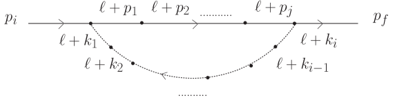
Figure 4: The general loop integral

We will define the general loop integral in $d$ dimensions containing $i$ pion propagators and $j$ nucleon propagators and corresponding to the momenta as in Fig. 4 as

$$I_{\pi\pi...\pi NN...N}[k_{1},k_{2},...,k_{i},p_{1},p_{2},...p_{j},A]=i\mu^{4-d}\int\frac{d^{d}\ell}{(2\pi)^{d}}\frac{A}{D_{\pi}(k_{1})...D_{\pi}(k_{i})D_{N}(p_{1})...D_{N}(p_{j})}\,.$$ (103)

Here $\mu$ is a scale factor and $A$ is the numerator function, which may contain anything. $D_{\pi}(k)=(\ell+k)^{2}-m_{0\pi}^{2}+i\epsilon$ and $D_{N}(p)=(\ell+p)^{2}-m^{2}+i\epsilon$ are respectively the pion and nucleon propagator denominators. $m_{0\pi}$ and $m$ are the unrenormalized pion and nucleon masses appearing in the original Lagrangian. Thus the number of subscripts $\pi$ and $N$ correspond to the number of pion and nucleon propagators respectively. We will always redefine the integration variable $\ell$ so as to make the first pion momentum $k_{1}=0$ and will drop it from the argument list.

In general we can always reduce $A$ to factors which can be removed from the integral or to powers of $\ell^{\mu}$, which at the one loop level can be reduced out using standard tensor expansions. Thus the only integrals which need to be evaluated explicitly have $A=1$.

For the basic calculation we need the integrals $I_{\pi}[1]$, $I_{\pi\pi}[q,1]$, $I_{N}[p,1]$, $I_{NN}[p_{i},p_{f},1]$, $I_{\pi N}[p,1]$, $I_{\pi NN}[p_{i},p_{f},1]$, $I_{\pi\pi N}[-q,p_{i},1]$. For those diagrams with a mass insertion on an internal nucleon diagram, which duplicates one of the nucleon propagators, we require the additional integrals $I_{NN}[p,p,1]$, $I_{NNN}[p_{i},p_{f},p_{f},1]$, $I_{NNN}[p_{i},p_{i},p_{f},1]$, $I_{\pi NN}[p,p,1]$, $I_{\pi NNN}[p_{i},p_{f},p_{f},1]$, $I_{\pi\pi NN}[-q,p_{i},p_{i},1]$, where $p$ can be either $p_{i}$ or $p_{f}$ and where $q=p_{f}-p_{i}$.

The evaluation of these integrals in the form needed for the IR or EOMS schemes proceeds in the standard fashion, as described for example in BL . The meson and nucleon propagators are separately combined using the Feynman parameter approach. The two pieces are then combined and the infinities extracted using standard dimensional regularization formalism. The results can then be expressed in $d$ dimensions in terms of the $R$ and $\epsilon=(4-d)/2$ of Eq. (56) and of relatively simple integrals over the Feynman parameters. This approach however leads, as discussed in the main text, to results which do not obey the usual HBChPT counting rules.

Becher and Leutwyler BL modify this procedure by dividing the integrals into two parts, one containing the infrared singularities and the other a regular polynomial in the expansion parameter. The regular part is then ’dropped’, i.e. in a formal sense absorbed in the LEC counterterms.

In order to discuss both the standard and the Becher-Leutwyler approach simultaneously we define a parameter $\beta^{IR}$ which flags the terms to be dropped in the Becher-Leutwyler procedure. Thus integrals involving only nucleons obtain an overall $\beta^{IR}$ in accord with the result that they are regular. Integrals with only pions are evaluated in the standard approach and so contain no $\beta^{IR}$. For those integrals involving both pions and nucleon propagators the basic integral on the parameter $z$ is divided into two parts and evaluated in accord with BL ; Sch04 as

$$\int_{0}^{1}dz\rightarrow\int_{0}^{\infty}dz\,-\,\beta^{IR}\int_{1}^{\infty}dz\,.$$ (104)

As discussed above, the singular terms proportional to $R$, which appear in both regular and infrared parts, can be recombined (i.e we eventually put $\beta^{IR}R\rightarrow R$) and the renormalization of the LEC’s carried out in the usual way. Thus $\beta^{IR}$ will serve to flag the regular terms which would be dropped in the Becher-Leutwyler procedure.

With these preliminaries recorded we can list the results for the integrals we need in this calculation.

$I_{\pi}[1]$, $I_{\pi\pi}[q,1]$, $I_{N}[p,1]$, and $I_{NN}[p_{i},p_{f},1]$ are standard and the results are given here for completeness only:

For $I_{\pi}[1]$

$$I_{\pi}[1]=\frac{m_{0\pi}^{2}}{(4\pi)^{2}}(R+{\rm ln}(\frac{m_{0\pi}^{2}}{\mu^{2}}))\,.$$ (105)

For $I_{\pi\pi}[q,1]$

$$I_{\pi\pi}[q,1]=\frac{1}{(4\pi)^{2}}(R+1+{\rm ln}(\frac{m_{0\pi}^{2}}{\mu^{2}}))+W_{\pi\pi}[q^{2}]\,,$$ (106)

with

$$W_{\pi\pi}[q^{2}] = \frac{1}{(4\pi)^{2}}\int_{0}^{1}dz\>{\rm ln}(D-i\eta)$$ (107)

$$= -\frac{q^{2}}{96\pi^{2}m_{0\pi}^{2}}-\frac{q^{4}}{960\pi^{2}m_{0\pi}^{4}}+....$$ (108)

where here

$$D=1-\frac{q^{2}}{m_{0\pi}^{2}}z(1-z)\,.$$ (109)

For $I_{N}[p,1]$

$$I_{N}[p,1]=I_{N}[0,1]=\beta^{IR}\frac{m^{2}}{(4\pi)^{2}}(R+{\rm ln}(\frac{m^{2}}{\mu^{2}}))\,.$$ (110)

For $I_{NN}[p_{i},p_{f},1]$

$$I_{NN}[p_{i},p_{f},1] = \beta^{IR}\frac{1}{(4\pi)^{2}}(R+1+{\rm ln}(\frac{m^{2}}{\mu^{2}}))+W_{NN}[q^{2}]\,,$$ (111)

$$I_{NN}[p,p,1] = I_{NN}[0,0,1]\ =\beta^{IR}\frac{1}{(4\pi)^{2}}(R+1+{\rm ln}(\frac{m^{2}}{\mu^{2}}))\,,$$ (112)

$$I_{NNN}[p_{i},p_{f},p_{f},1] = I_{NNN}[p_{i},p_{i},p_{f},1]=W_{NNN}[q^{2}]\,,$$ (113)

with

$$W_{NN}[q^{2}] = \beta^{IR}\frac{1}{(4\pi)^{2}}\int_{0}^{1}dz\>{\rm ln}(D-i\eta)$$ (114)

$$= \beta^{IR}(-\frac{q^{2}}{96\pi^{2}m_{N}^{2}}+\frac{\delta_{m}q^{2}m_{0\pi}^{2}}{96\pi^{2}m_{N}^{4}}-\frac{q^{4}}{960\pi^{2}m_{N}^{4}}+....)\,,$$ (115)

$$W_{NNN}[q^{2}] = \frac{\beta^{IR}}{(4\pi)^{2}m^{2}}\int_{0}^{1}\frac{dz}{D-i\eta}$$ (116)

$$= \beta^{IR}(\frac{1}{32\pi^{2}m_{N}^{2}}-\frac{\delta_{m}m_{0\pi}^{2}}{32\pi^{2}m_{N}^{4}}+\frac{q^{2}}{192\pi^{2}m_{N}^{4}}+....)$$ (117)

where here

$$D=1-\frac{q^{2}}{m^{2}}z(1-z)\quad{\rm and}\quad\delta_{m}=\frac{m^{2}-m_{N}^{2}}{m_{0\pi}^{2}}\,.$$ (118)

For simplicity we have given only the first few terms in the expansions of the $W$’s above, as the full expressions used are quite lengthy. In the actual calculations we kept more terms, as many as necessary to obtain the final amplitude through the first four orders in the expansion parameter.

The remaining integrals involve both pion and nucleon propagators. For those we follow and generalize the procedure used in BL for $I_{\pi N}$.

For $I_{\pi N}[p,1]$ we find, after combining denominators and evaluating via dimensional regularization,

$$I_{\pi N}[p,1]=-\frac{1}{(4\pi)^{2}}(R-1+{\rm ln}(\frac{m^{2}}{\mu^{2}}))(2\epsilon-1)\int_{0}^{1}\frac{dz}{(C-i\eta)^{\epsilon}}\,.$$ (119)

Here $C=C_{0}+C_{1}(z-z_{0})^{2}$. For this case $C_{1}=1+2\alpha\Omega+\alpha^{2}$, $C_{0}=\alpha^{2}(1-\Omega^{2})/C_{1}$ and $z_{0}=\alpha(\alpha+\Omega)/C_{1}$. Here (and below) $\alpha=m_{0\pi}/m$ and $\Omega=(p^{2}-m^{2}-m_{0\pi}^{2})/(2mm_{0\pi})$. These integrals depend on the square of the four momentum $p^{2}$ but we will need them only at the physical on shell point $p^{2}=m_{N}^{2}$. We must account for the fact that $m\neq m_{N}$ and hence as above use $m^{2}-m_{N}^{2}\equiv\delta_{m}m_{0\pi}^{2}$ where $\delta_{m}$ is a dimensionless parameter presumedly of order one. In fact, from Appendix B we have $\delta_{m}=8c_{1}m_{N}+...$. This allows us to expand in powers of $m_{0\pi}$ about the physical mass $m_{N}$. The integral can be done analytically, basically by integrating by parts, as in BL and we obtain

$$I_{\pi N}[p,1]=\frac{R}{(4\pi)^{2}}(\beta^{IR}-\frac{m_{0\pi}^{2}}{2m_{N}^{2}}(\beta^{IR}-1)(1-\delta_{m}))+W_{\pi N}[p^{2},m^{2},m_{0\pi}^{2}]\,,$$ (120)

where on shell

$$W_{\pi N}[m_{N}^{2},m^{2},m_{0\pi}^{2}] = \frac{\beta^{IR}}{16\pi^{2}}({\rm ln}(\frac{m_{N}^{2}}{\mu^{2}})-1)+\frac{m_{0\pi}}{16\pi m_{N}}+\frac{m_{0\pi}^{2}}{32\pi^{2}m_{N}^{2}}(1-3\beta^{IR}$$ (121)

$$+\delta_{m}(\beta^{IR}-1)+(1-\delta_{m})({\rm ln}(\frac{m_{0\pi}^{2}}{\mu^{2}})-\beta^{IR}{\rm ln}(\frac{m_{N}^{2}}{\mu^{2}})))+....\,.$$

In a similar fashion we find for $I_{\pi NN}[p_{i},p_{f},1]$,$I_{\pi NNN}[p_{i},p_{f},p_{f},1]$, and $I_{\pi NNN}[p_{i},p_{i},p_{f},1]$

$$I_{\pi NN}[p_{i},p_{f},1] = -\frac{1}{2m^{2}(4\pi)^{2}}(R+1+{\rm ln}(\frac{m^{2}}{\mu^{2}}))(2\epsilon)\int_{0}^{1}dy\int_{0}^{1}\frac{z\>dz}{(C-i\eta)^{1+\epsilon}}\,,$$ (122)

$$I_{\pi NNN}[p_{i},p_{f},p_{f},1] = I_{\pi NNN}[p_{i},p_{i},p_{f},1]$$ (123)

$$= -\frac{1}{m^{4}(4\pi)^{2}}(1+2\epsilon)\int_{0}^{1}ydy\int_{0}^{1}\frac{z^{2}dz}{(C-i\eta)^{2+\epsilon}}\,,$$

where now on shell with $p_{i}^{2}=p_{f}^{2}=m_{N}^{2}$, $C_{1}=1+2\alpha\Omega+\alpha^{2}-y(1-y)q^{2}/m^{2}$, $C_{0}=\alpha^{2}(1-\Omega^{2}-y(1-y)q^{2}/m^{2})/C_{1}$ and $z_{0}=\alpha(\alpha+\Omega)/C_{1}$. The integrals on $z$ can be obtained analytically by generalizing the procedure of BL . This result is then expanded in powers of the small parameter and integrated term by term on $y$. We thus obtain

$$I_{\pi NN}[p_{i},p_{f},1] = W_{\pi NN}[p_{i}^{2},p_{f}^{2},q^{2},m^{2},m_{0\pi}^{2}]\,,$$ (124)

$$I_{\pi NNN}[p_{i},p_{f},p_{f},1] = I_{\pi NNN}[p_{i},p_{i},p_{f},1]=\frac{1}{m_{0\pi}}W_{\pi NNN}[p_{i}^{2},p_{f}^{2},q^{2},m^{2},m_{0\pi}^{2}]\,,$$ (125)

where on shell

$$W_{\pi NN}[m_{N}^{2},m_{N}^{2},q^{2},m^{2},m_{0\pi}^{2}] = \frac{\beta^{IR}-1}{32\pi^{2}m_{N}^{2}}+\frac{1}{32\pi^{2}m_{N}^{2}}(\beta^{IR}{\rm ln}(\frac{m_{N}^{2}}{\mu^{2}})-{\rm ln}(\frac{m_{\pi}^{2}}{m_{N}^{2}}))$$ (126)

$$+ \frac{m_{0\pi}}{64\pi m_{N}^{3}}(1-\delta_{m})+\frac{m_{0\pi}^{2}}{64\pi^{2}m_{N}^{4}}(1-2\beta^{IR})(1-2\delta_{m})$$

$$+ \frac{m_{0\pi}^{2}\delta_{m}^{2}}{64\pi^{2}m_{N}^{4}}-\frac{q^{2}}{192\pi^{2}m_{N}^{4}}(1+{\rm ln}(\frac{m_{\pi}^{2}}{m_{N}^{2}})$$

$$- \beta^{IR}{\rm ln}(\frac{m_{N}^{2}}{\mu^{2}}))+.....\,,$$

$$W_{\pi NNN}[m_{N}^{2},m_{N}^{2},q^{2},m^{2},m_{0\pi}^{2}] = -\frac{1}{128\pi m_{N}^{3}}-\frac{m_{0\pi}}{64\pi^{2}m_{N}^{4}}(1-2\beta^{IR}-\delta_{m})$$ (127)

$$- \frac{3m_{0\pi}^{2}}{1024\pi m_{N}^{5}}(1-6\delta_{m}+\delta_{m}^{2})-\frac{q^{2}}{512\pi m_{N}^{5}}+...\,.$$

The $\pi NN$ integral with duplicate nucleon propagators can be obtained by taking $q^{2}\rightarrow 0$ in $I_{\pi NN}[p_{i},p_{f},1]$, namely

$$I_{\pi NN}[p,p,1]=W_{\pi NN}[m_{N}^{2},m_{N}^{2},0,m^{2},m_{0\pi}^{2}]\,.$$ (128)

Finally

$$I_{\pi\pi N}[-q,p_{i},1] = -\frac{1}{2m^{2}(4\pi)^{2}}(R+1+{\rm ln}(\frac{m^{2}}{\mu^{2}}))(2\epsilon)\int_{0}^{1}dx\int_{0}^{1}\frac{(1-z)dz}{(C-i\eta)^{1+\epsilon}}\,,$$ (129)

$$I_{\pi\pi NN}[-q,p_{i},p_{i},1] = -\frac{1}{m^{4}(4\pi)^{2}}(1+2\epsilon)\int_{0}^{1}dx\int_{0}^{1}\frac{(1-z)zdz}{(C-i\eta)^{2+\epsilon}}\,,$$ (130)

where we now have on shell with $p_{i}^{2}=m_{N}^{2}$, $C_{1}=1+2\alpha\Omega+\alpha^{2}-x(1-x)q^{2}/m^{2}$, $C_{0}=\alpha^{2}-C_{1}z_{0}^{2}-x(1-x)q^{2}/m^{2}$ and $z_{0}=\alpha(\alpha+\Omega)/C_{1}-x(1-x)q^{2}/(m^{2}C_{1})$. footnote3 Again we can do the $z$ integration analytically and then expand in powers of the small parameter and do the $x$ integration term by term. We then obtain

$$I_{\pi\pi N}[-q,p_{i},1] = \frac{1}{m_{0\pi}}W_{\pi\pi N}[p_{i}^{2},p_{f}^{2},q^{2},m^{2},m_{0\pi}^{2}]\,,$$ (131)

$$I_{\pi\pi NN}[-q,p_{i},p_{i},1] = \frac{1}{m_{0\pi}^{2}}W_{\pi\pi NN}[p_{i}^{2},p_{f}^{2},q^{2},m^{2},m_{0\pi}^{2}]\,,$$ (132)

where on shell

$$W_{\pi\pi N}[m_{N}^{2},m_{N}^{2},q^{2},m^{2},m_{0\pi}^{2}] = \frac{1}{32\pi m_{N}}(1+\frac{q^{2}}{12m_{0\pi}^{2}})$$ (133)

$$+ \frac{m_{0\pi}}{32\pi^{2}m_{N}^{2}}(2-\delta_{m}-3\beta^{IR}+{\rm ln}(\frac{m_{\pi}^{2}}{m_{N}^{2}})-\beta^{IR}{\rm ln}(\frac{m_{N}^{2}}{\mu^{2}}))$$

$$- \frac{q^{2}}{192\pi^{2}m_{N}^{2}m_{0\pi}}(1+\delta_{m})+.....\,,$$

$$W_{\pi\pi NN}[m_{N}^{2},m_{N}^{2},q^{2},m^{2},m_{0\pi}^{2}] = -\frac{1}{32\pi^{2}m_{N}^{2}}(1+\frac{q^{2}}{6m_{0\pi}^{2}})+\frac{m_{0\pi}}{128\pi m_{N}^{3}}(1+\delta_{m})$$ (134)

$$+ \frac{q^{2}}{1536\pi m_{N}^{3}m_{0\pi}}(1+3\delta_{m})+....\,.$$

Finally we observe that there is an alternative method for obtaining the loop integrals involving two nucleon propagators of the same momentum. It follows from the relations

$$\frac{\partial}{\partial m^{2}}\{\frac{1}{p^{2}-m^{2}}\}=\{\frac{1}{p^{2}-m^{2}}\}^{2},\quad\quad\frac{\partial}{\partial m^{2}}=\frac{1}{m_{0\pi}^{2}}\frac{\partial}{\partial\delta_{m}}$$ (135)

that one can get a loop integral with a duplicate propagator by taking derivatives, namely

$$\frac{1}{m_{0\pi}^{2}}\frac{\partial}{\partial\delta_{m}}I_{\pi N}[p,1] = I_{\pi NN}[p,p,1]\,,$$ (136)

$$\frac{1}{m_{0\pi}^{2}}\frac{\partial}{\partial\delta_{m}}I_{NN}[p_{i},p_{f},1] = I_{NNN}[p_{i},p_{f},p_{f},1]+I_{NNN}[p_{i},p_{i},p_{f},1]\,,$$ (137)

$$\frac{1}{m_{0\pi}^{2}}\frac{\partial}{\partial\delta_{m}}I_{\pi NN}[p_{i},p_{f},1] = I_{\pi NNN}[p_{i},p_{f},p_{f},1]+I_{\pi NNN}[p_{i},p_{i},p_{f},1]\,,$$ (138)

$$\frac{1}{m_{0\pi}^{2}}\frac{\partial}{\partial\delta_{m}}I_{\pi\pi N}[-q,p_{i},1] = I_{\pi\pi NN}[-q,p_{i},p_{i},1]\,.$$ (139)

We have checked that our results satisfy these relations. Note that to obtain $I_{\pi NN}[p,p,1]$ for example to ${\cal O}(m_{\pi}^{4})$ we need $I_{\pi N}[p,1]$ to ${\cal O}(m_{\pi}^{6})$ because of the $m_{\pi}^{2}$ introduced in the denominator by the derivative. This somewhat lessens the utility of this method for actually calculating the integrals with duplicate propagators.

Appendix B Mass and wave function renormalization

In the meson sector the pion mass and wave function renormalizations are calculated in standard fashion and are given in a number of sources, for example, fear97 . In our conventions and notation we have

$$m_{\pi}^{2}=m_{0\pi}^{2}\left[1+\frac{2m_{\pi}^{2}}{F_{\pi}^{2}}\left(l_{3}^{r}(\mu)+\frac{1}{4(4\pi)^{2}}{\rm ln}\left(\frac{m_{\pi}^{2}}{\mu^{2}}\right)\right)\right],$$ (140)

and

$$Z_{\pi}=1-\frac{2m_{\pi}^{2}}{F_{\pi}^{2}}\left[l_{4}^{r}(\mu)+\frac{2}{3(4\pi)^{2}}R-\frac{1}{3(4\pi)^{2}}{\rm ln}\left(\frac{m_{\pi}^{2}}{\mu^{2}}\right)\right]~{}.$$ (141)

where the LEC’s have been renormalized as

$$l_{3}^{r}(\mu) = l_{3}+\frac{R}{4(4\pi)^{2}}\,,$$ (142)

$$l_{4}^{r}(\mu) = l_{4}-\frac{R}{(4\pi)^{2}}\,.$$ (143)

The renormalization of the pion decay constant is also standard and given from fear97 by

$$F_{\pi}=F_{0}\left[1+\frac{m_{\pi}^{2}}{F_{\pi}^{2}}\left(l_{4}^{r}(\mu)-\frac{1}{(4\pi)^{2}}{\rm ln}\left(\frac{m_{\pi}^{2}}{\mu^{2}}\right)\right)\right]~{}.$$ (144)

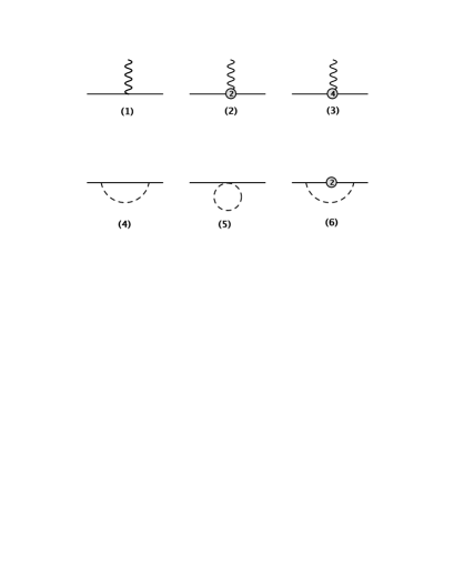
Figure 5: Diagrams contributing to the nucleon self energy

In the pion-nucleon sector the nucleon mass and wave function renormalizations must be calculated in a fashion consistent with the rest of the calculation. The appropriate diagrams contributing to the nucleon self energy are given in Fig. 5 and the amplitudes corresponding to those figures are given by

$$M_{1NN} = i\overline{\Psi}(\not\!p-m)\Psi\,,$$ (145)

$$M_{2NN} = i\overline{\Psi}(4c_{1}m_{0\pi}^{2})\Psi\,,$$ (146)

$$M_{3NN} = i\overline{\Psi}(2m_{0\pi}^{4}(8e_{38}+e_{115}+e_{116}))\Psi\,,$$ (147)

$$M_{4NN} = -\frac{3ig_{A}^{2}}{4F_{0}^{2}}\overline{\Psi}I_{\pi N}[p,\not\!\ell\gamma_{5}(\not\!p+\not\!\ell+m)\not\!\ell\gamma_{5})]\Psi\,,$$ (148)

$$M_{5NN} = -\frac{3im_{0\pi}^{2}}{F_{0}^{2}}\overline{\Psi}(2c_{1}-c_{3}-\frac{c_{2}p^{2}}{dm_{N}^{2}})\Psi I_{\pi}[1]\,,$$ (149)

$$M_{6NN} = -\frac{3ig_{A}^{2}}{4F_{0}^{2}}(-4c_{1}m_{0\pi}^{2})\overline{\Psi}I_{\pi NN}[p,p,\not\!\ell\gamma_{5}(\not\!p+\not\!\ell+m)(\not\!p+\not\!\ell+m)\not\!\ell\gamma_{5}]\Psi\,.$$ (150)

We evaluate these amplitudes using standard dimensional regularization and expand the integrals in powers of the small momentum, keeping for now the finite terms which do not obey counting. As discussed above those finite terms which would be dropped in the Becher-Leutwyler procedure are flagged with the symbol $\beta^{IR}$. Likewise we flag terms from each diagram which would be dropped in the EOMS procedure with $\beta^{EOMS}$.

A first renormalization of the low energy constants is required to ensure that the difference between the physical nucleon mass $m_{N}$ and the nucleon mass in the chiral limit $\stackrel{{\scriptstyle\circ}}{{m_{N}}}$ is finite. In particular we take

$$c_{1}^{r} = c_{1}+\frac{3g_{A}^{2}m_{N}R}{128F_{\pi}^{2}\pi^{2}}(1-12c_{1}m_{N})\,,$$ (151)

$$e_{115}^{r}+e_{116}^{r}+8e_{38}^{r} = e_{115}+e_{116}+8e_{38}+\frac{3R}{128F_{\pi}^{2}\pi^{2}}(c_{2}-8c_{1}+4c_{3}-168c_{1}^{2}m_{N}g_{A}^{2})\,.$$ (152)

The finite renormalizations required read

$$c_{1}^{IR} = c_{1}^{EOMS}\,,$$ (153)

$$e_{115}^{IR}+e_{116}^{IR}+8e_{38}^{IR} = e_{115}^{EOMS}+e_{116}^{EOMS}+8e_{38}^{EOMS}-\frac{3{c_{1}}^{2}m_{N}g_{A}^{2}}{16F_{\pi}^{2}\pi^{2}}(28+15{\rm ln}(m_{N}^{2}/\mu^{2}))$$ (154)

$$-\frac{3g_{A}^{2}}{128F_{\pi}^{2}\pi^{2}m_{N}}(3+{\rm ln}(m_{N}^{2}/\mu^{2}))\,,$$

and

$$c_{1}^{EOMS} = c_{1}^{r}-\frac{3m_{N}g_{A}^{2}}{128F_{\pi}^{2}\pi^{2}}(1+8c_{1}m_{N}-(1-12c_{1}m_{N}){\rm ln}(m_{N}^{2}/\mu^{2}))\,,$$ (155)

$$e_{115}^{EOMS}+e_{116}^{EOMS}+e_{38}^{EOMS} = e_{115}^{r}+e_{116}^{r}+8e_{38}^{r}-\frac{3{c_{1}}^{2}m_{N}g_{A}^{2}}{8F_{\pi}^{2}\pi^{2}}(8+3{\rm ln}(m_{N}^{2}/\mu^{2}))\,.$$ (156)

This leads to

$$m_{N} = \left[m-\frac{3g_{A}^{2}m^{3}}{32F_{\pi}^{2}\pi^{2}}(R+{\rm ln}(m^{2}/\mu^{2}))\right]-4m_{\pi}^{2}c_{1}^{IR}-2m_{\pi}^{4}(e_{115}^{IR}+e_{116}^{IR}+8e_{38}^{IR})$$ (157)

$$-\frac{3g_{A}^{2}m_{\pi}^{3}}{32F_{\pi}^{2}\pi}-\frac{3g_{A}^{2}m_{\pi}^{4}}{64F_{\pi}^{2}\pi^{2}m_{N}}(1+{\rm ln}(m_{\pi}^{2}/\mu^{2}))+\frac{3c_{2}m_{\pi}^{4}}{128F_{\pi}^{2}\pi^{2}}$$

$$-\frac{m_{\pi}^{4}}{64F_{\pi}^{2}\pi^{2}}(3c_{2}-32c_{1}+12c_{3}){\rm ln}(m_{\pi}^{2}/\mu^{2})+\frac{8c_{1}m_{\pi}^{4}}{F_{\pi}^{2}}l_{3}^{r}(\mu)\,.$$

Observe that all of the terms in the above formula which are proportional to $1/F_{\pi}^{2}$ do not contribute to any physical amplitude we calculate here. They would lead to $1/F_{\pi}^{4}$ corrections to loop diagrams, the same order as two loop contributions which we are neglecting. Furthermore the tree level diagrams do not contain nucleon masses for which these terms are relevant. Thus for practical purposes we can take

$$m\rightarrow m_{N}+4c_{1}m_{\pi}^{2}+2m_{\pi}^{4}(e_{115}+e_{116}+8e_{38})\,,$$ (158)

where we have dropped all terms with $1/F_{\pi}^{2}$, which also allows $\{c_{1}^{IR},e_{115}^{IR},e_{116}^{IR},e_{38}^{IR}\}\rightarrow\{c_{1},e_{115},e_{116},e_{38}\}$.

Note also that in the chiral limit only the $R$ term survives, i.e. we obtain

$$\stackrel{{\scriptstyle\circ}}{{m_{N}}}=m-\frac{3g_{A}^{2}m^{3}}{32F_{\pi}^{2}\pi^{2}}(R+{\rm ln}(m^{2}/\mu^{2}))\,.$$ (159)

It is common to introduce explicitly or implicitly a counterterm in the Lagrangian to eliminate the correction term in this formula and thus to interpret $m$ from the beginning as the nucleon mass in the chiral limit, $\stackrel{{\scriptstyle\circ}}{{m_{N}}}$, rather than as a ’bare’ mass as we have done.

Finally the nucleon wave function renormalization becomes

$$Z_{N} = 1-\frac{3m_{\pi}^{2}g_{A}^{2}}{64F_{\pi}^{2}\pi^{2}}\left(2(1+\beta^{IR})+(3-2\beta^{IR})R+16c_{1}m_{N}\beta^{IR}(\beta^{EOMS}-1)\right.$$ (160)

$$+\left.3{\rm ln}(\frac{m_{\pi}^{2}}{\mu^{2}})-2\beta^{IR}(1-6c_{1}m_{N}(1-\beta^{EOMS})){\rm ln}(\frac{m_{N}^{2}}{\mu^{2}})-\frac{3m_{\pi}\pi}{m_{N}}\right)$$

If we reexpress the formulas for $m_{N}$ and $Z_{N}$ in terms of $m$ and $m_{0\pi}$ and take $\mu=m$ and take $\beta^{IR}=0$ then these results agree with those of Ref. BL . Note however that there are no LEC’s or counterterms available to absorb the $\beta^{IR}$ or $\beta^{EOMS}$ terms in $Z_{N}$, i.e. those terms which are to be dropped in the IR or EOMS schemes. Instead what happens is that these terms enter the amplitudes via the $\sqrt{Z_{N}}$ terms which appear in Eqs. (15),(16),(17),(45) and are absorbed in LEC’s elsewhere in the calculation.

References

- (1) T. Gorringe and H. W. Fearing, Rev. Mod. Phys. 76, 31 (2004).
- (2) V. Bernard, L. Elouadrhiri, and U.-G. Meißner, J. Phys. G 28, R1 (2002).
- (3) D. F. Measday, Phys. Rep. 354, 243 (2001).
- (4) S. Weinberg, Physica A 96, 327 (1979).
- (5) H. W. Fearing, R. Lewis, N. Mobed, and S. Scherer, Phys. Rev. D 56, 1783 (1997).
- (6) S. Ando, F. Myhrer, and K. Kubodera, Phys. Rev. C 63, 015203 (2001).
- (7) V. Bernard, T. R. Hemmert, and U.-G. Meißner, Nucl. Phys. A 686, 290 (2001).
- (8) V. Bernard, H. W. Fearing, T. R. Hemmert, and U.-G. Meissner, Nucl. Phys. A635, 121 (1998); (E) A642, 563 (1998).
- (9) S. Scherer, in Advances in Nuclear Physics, Vol. 27, edited by J. W. Negele and E. W. Vogt (Kluwer Academic/Plenum Publishers, New York, 2003).
- (10) T. Fuchs, J. Gegelia, G. Japaridze, and S. Scherer, Phys. Rev. D 68 056005 (2003).
- (11) M. R. Schindler, J. Gegelia, S. Scherer, Phys. Lett. B586, 258 (2004).
- (12) T. Becher and H. Leutwyler, Eur. Phys. J. C9, 643 (1999).
- (13) P. J. Ellis and H.-B. Tang, Phys. Rev. C 57, 3356 (1998).
- (14) J. Gegelia, G. Japaridze, and X. Q. Wong, J. Phys. G 29, 2309 (2003).
- (15) Strictly speaking these are manifestly Lorentz invariant theories rather than fully relativistic. They use relativistic propagators and the full machinery of Dirac algebra, but they do not include antiparticles as explicit degrees of freedom and in particular do not include nucleon or anti nucleon loops. We will refer to these theories somewhat imprecisely as ’relativistic’ or ’manifestly Lorentz invariant’ ChPT or as ’relativistic baryon ChPT’, or simply ’baryon ChPT’ (BChPT).
- (16) J. Gasser, M. E. Sainio, and A. Švarc, Nucl. Phys. B 307, 779 (1988).
- (17) T. Becher and H. Leutwyler, J. High Energy Phys. JHEP06, 017 (2001).
- (18) T. Fuchs, J. Gegelia, and S. Scherer, J. Phys. G 30, 1407 (2004).
- (19) T. Fuchs, Formfaktoren des Nukleons in relativistischer chiraler Störungstheorie, Ph.D Thesis, J. G. Universität Mainz, 2002.
- (20) B. Kubis and U.-G. Meißner, Nucl. Phys. A 679, 698 (2001).
- (21) J. Schweizer, Low Energy Representation for the Axial Form Factor of the Nucleon, Diplomarbeit, Universität Bern, 2000.
- (22) H. W. Fearing, T. R. Hemmert, R. Lewis, and C. Unkmeir, Phys. Rev. C 62, 054006 (2000); H. W. Fearing, T. R. Hemmert, R. Lewis, and C. Unkmeir, Chiral Dynamics: Theory and Experiment III, ed. by A. M. Bernstein, J. L. Goity and Ulf-G. Meissner, World Scientific, (2001) 380; H. W. Fearing, T. R. Hemmert, R. Lewis, and C. Unkmeir, Nucl. Phys. A684, 377 (2001).
- (23) T. Meissner, F. Myhrer, and K. Kubodera, Phys. Lett. B 416, 36 (1998).
- (24) S. Ando and D.-P. Min, Phys. Lett. B 417, 177 (1998).
- (25) S. Ando, H. W. Fearing, and D.-P. Min, Phys. Rev. C 65, 015502 (2002).
- (26) E. Truhlík and F. C. Khanna, Phys. Rev. C 65, 045504 (2002).
- (27) S. Ando, F. Myhrer, and K. Kubodera, Phys. Rev. C 65, 048501 (2002).
- (28) J. D. Bjorken and S. D. Drell, Relativistic Quantum Mechanics, (McGraw-Hill, N.Y.), 1964.
- (29) S. Ando et al., Phys. Lett. B 595, 250 (2004).
- (30) Particle Data Group, J. Phys. G 33, 1 (2006).
- (31) N. Fettes, U.-G. Meißner, M. Mojžiš, S. Steininger, Annals Phys. 283, 273 (2000); Erratum ibid 288, 249 (2001).
- (32) J. Gasser and H. Leutwyler, Ann. Phys. (N.Y.) 158, 142 (1984).
- (33) D. Djukanovic, M. R. Schindler, J. Gegelia, and S. Scherer, Phys. Rev. D 72, 045002 (2005).
- (34) It should be always be clear from context that the integration variable is different from the current defined earlier.
- (35) P. Mergell, Ulf-G. Meissner, and D. Drechsel, Nucl. Phys. A 596, 367 (1996).
- (36) L. A. Ahrens et al., Phys. Lett. B 202, 284 (1988).
- (37) V. Stoks, R. Timmermans, and J. J. de Swart, Phys. Rev. C 47, 512 (1993).
- (38) A. Sirlin, Phys. Rev. 164, 1767 (1967).
- (39) W. J. Marciano and A. Sirlin, Phys. Rev. Lett. 56, 22 (1986).
- (40) C. Hacker, N. Wies, J. Gegelia, S. Scherer, Phys. Rev. C 72, 055203 (2005).
- (41) V. Bernard, T. Hemmert, and Ulf-G. Meissner, Phys. Lett. B565, 137 (2003).
- (42) M. R. Schindler, J. Gegelia, S. Scherer, Eur. Phys. J. A26, 1 (2005).
- (43) D. Binosi and L. Theussl, Computer Physics Communications, 161, 76 (2004).
- (44) To obtain or , which are not actually needed for this calculation, one must take in these formulas, but also in and . This latter change results because are not all independent parameters, but are related via .