$B_{s}^{0}$-$\bar{B}_{s}^{0}$ MIXING IN THE MSSM WITH LARGE $\tan\beta$

Abstract

The $B_{s}$-$\bar{B}_{s}$ mixing parameter $\Delta M_{s}$ is studied in the MSSM with large $\tan\beta$. The recent Tevatron measurement of $\Delta M_{s}$ is used to constrain the MSSM parameter space. From this analysis the often neglected contribution to $\Delta M_{s}$ from the operator $Q^{SLL}_{1}$ is found to be significant.

Received 11 October 2006

PACS Nos.: 14.40.Nd, 12.60.Jv

1 Introduction

In the Standard Model(SM) flavour changing neutral current(FCNC) processes are absent at tree-level and only enter at higher orders. In extensions of the SM there exist numerous additional sources of FCNC. A clear example comes from the mixings present in the squark sector of the Minimal Supersymmetric Standard Model(MSSM). These mixings will also contribute to FCNCs at the one-loop level and could even be larger than their SM counterparts. An example that we shall study in this work is the flavour changing couplings of neutral Higgs bosons and the neutral Higgs penguin contribution to such decays as $B_{s}^{0}\to\mu^{+}\mu^{-}$ and $B_{s}^{0}\!-\!\bar{B}_{s}^{0}$ mixing. It is clear that such FCNC processes are an ideal place to search for physics beyond the Standard Model. Since the recent measurement of $\Delta M_{s}$ at the Tevatron[1, 2] its consequences have been studied model independently[3, 4, 5], in the MSSM[6, 7, 8, 9, 10], with minimal flavour violation[11], in GUTs[12, 13], in $Z^{\prime}$ models[14, 15, 16], with R-parity violation[17, 18, 19], two Higgs doublet models[20] and warped extra dimensions[21].

In this work $B_{s}$-$\bar{B}_{s}$ mixing is studied via two methods. The first analysis is based on the simple SUSY SU(5) model studied recently[22]. The second case is that of the MSSM Higgs sector making use of the FeynHiggs numerical package.

1.1 $\Delta M_{s}$ in the large $\tan\beta$ limit

It has been pointed out that Higgs mediated FCNC processes could be among the first signals of supersymmetry(SUSY)[23, 24, 25]. In the MSSM radiatively induced couplings between the up Higgs, $H_{u}$, and down-type quarks may result in flavour changing Higgs couplings. In turn this will lead to large FCNC decay rates for such process as $B_{s}\to\mu^{+}\mu^{-}$ and $B_{s}^{0}\!-\!\bar{B}_{s}^{0}$ mixing.

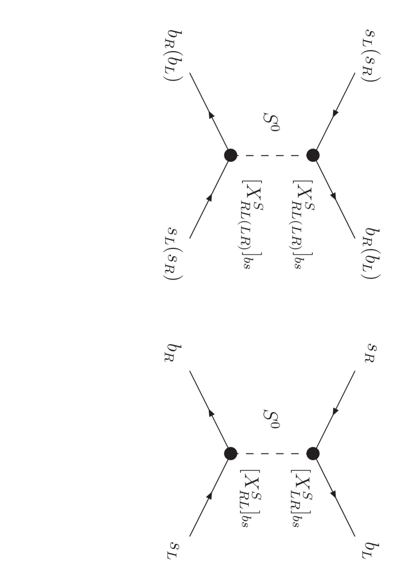
Figure 1: Higgs Penguin contributions to $\Delta M_{s}$ via the operators $Q_{1}^{SLL}(Q_{1}^{SRR})$ and $Q_{2}^{LR}$.

In the MSSM, loop diagrams will induce flavour changing couplings of the form, $b^{c}sH_{u}^{0*}$. Similar diagrams with Higgs fields replaced by their VEVs will also provide down quark mass corrections and will lead to sizeable corrections to the mass eigenvalues[26, 27, 28] and mixing matrices[29]. As a result the 3-point coupling and mass matrix can not be simultaneously diagonalised[30] and hence beyond tree-level we shall have flavour changing Higgs couplings in the mass eigenstate basis. Such flavour changing Higgs couplings can be summarized as,

$${\mathcal{L}}_{FCNC}\;=\;-\overline{d}_{R\,i}\left[X^{S}_{RL}\right]_{ij}d_{L\,j}\,S^{0}-\overline{d}_{L\,i}\left[X^{S}_{LR}\right]_{ij}d_{R\,j}\,S^{0}\,.$$ (1)

These flavour changing couplings can in fact be related in a simple way to the finite non-logarithmic mass matrix corrections[31],

$$\left[X^{S}_{RL}\right]_{ij}=\frac{1}{\sqrt{2}}\frac{1}{c_{\beta}}\left(\frac{\delta m_{d}^{finite}}{v_{u}}\right)_{ij}\,A_{S^{0}}$$ (2)

where, $A_{S^{0}}=\left(s_{\alpha-\beta},\,c_{\alpha-\beta},\,-i\right)$, for $S^{0}=\left(H^{0},\,h^{0},\,A^{0}\right)$. It is clear that the FCNC couplings are related as, $\left[X_{RL}\right]=\left[X_{LR}\right]^{\dagger}$. In general we should also notice that, $\left[X_{RL}\right]_{ij}\approx\frac{m_{i}}{m_{j}}\left[X_{RL}\right]_{ji}$. Hence, in the case of, $(i,\,j)=(b,\,s)$, we have $\left[X_{RL}\right]_{bs}\approx\frac{m_{b}}{m_{s}}\left[X_{LR}\right]_{bs}$.

In the MSSM with large $\tan\beta$ the dominant contribution to $B_{s}\to\ell^{+}\ell^{-}$ comes from the penguin diagram where the dilepton pair is produced from a virtual Higgs state. The Higgs Double Penguin(DP) contribution to $B_{s}^{0}\!-\!\bar{B}_{s}^{0}$ mixing, shown in fig. 1 is also the dominant SUSY contribution in the large $\tan\beta$ limit[32, 33]. Following the notation of eq. (1), we can write the neutral Higgs contribution to the $\Delta B=\Delta S=2$ effective Hamiltonian as,

$${\mathcal{H}}_{\sf eff}^{\Delta B=\Delta S=2} = \frac{1}{2}\sum_{S}\,\frac{[X^{S}_{RL}]_{bs}[X^{S}_{RL}]_{bs}}{-M_{S}^{2}}\,\,Q_{1}^{SLL}+\frac{1}{2}\sum_{S}\,\frac{[X^{S}_{LR}]_{bs}[X^{S}_{LR}]_{bs}}{-M_{S}^{2}}\,\,Q_{1}^{SRR}$$ (3)

$$\,\,\,\,+\sum_{S}\,\frac{[X^{S}_{RL}]_{bs}[X^{S}_{LR}]_{bs}}{-M_{S}^{2}}\,\,Q_{2}^{LR}$$

where we have defined the operators,

$$Q_{1}^{SLL} = (\overline{b}P_{L}s)\,(\overline{b}P_{L}s)$$

$$Q_{1}^{SRR} = (\overline{b}P_{R}s)\,(\overline{b}P_{R}s)$$ (4)

$$Q_{2}^{LR} = (\overline{b}P_{L}s)\,(\overline{b}P_{R}s)$$

The Higgs sum in eq. (3) leads to a factor, ${\mathcal{F}}^{\pm}=\left(\frac{s_{\alpha-\beta}^{2}}{M_{H}^{2}}+\frac{c_{\alpha-\beta}^{2}}{M_{h}^{2}}\pm\frac{1}{M_{A}^{2}}\right)$. The operators $Q_{1}^{SLL,SRR}$ receive the factor ${\mathcal{F}}^{-}$, while $Q_{2}^{LR}$ receives ${\mathcal{F}}^{+}$. The additional minus sign leads to a suppression of the $Q_{1}^{SLL,SRR}$ operators relative to $Q_{2}^{LR}$. At this point it is common to assume that the $Q_{1}^{SLL,SRR}$ contributions are negligible. Recalling that, $[X_{LR}]_{bs}\sim\frac{1}{40}[X_{RL}]_{bs}$, even for a suppression of ${\mathcal{F}}^{-}/{\mathcal{F}}^{+}\sim 1/100$, it may be possible for the $Q_{1}^{SLL}$ contribution to give a significant effect. On the other hand, the contribution to $Q_{1}^{SRR}$ is highly suppressed.

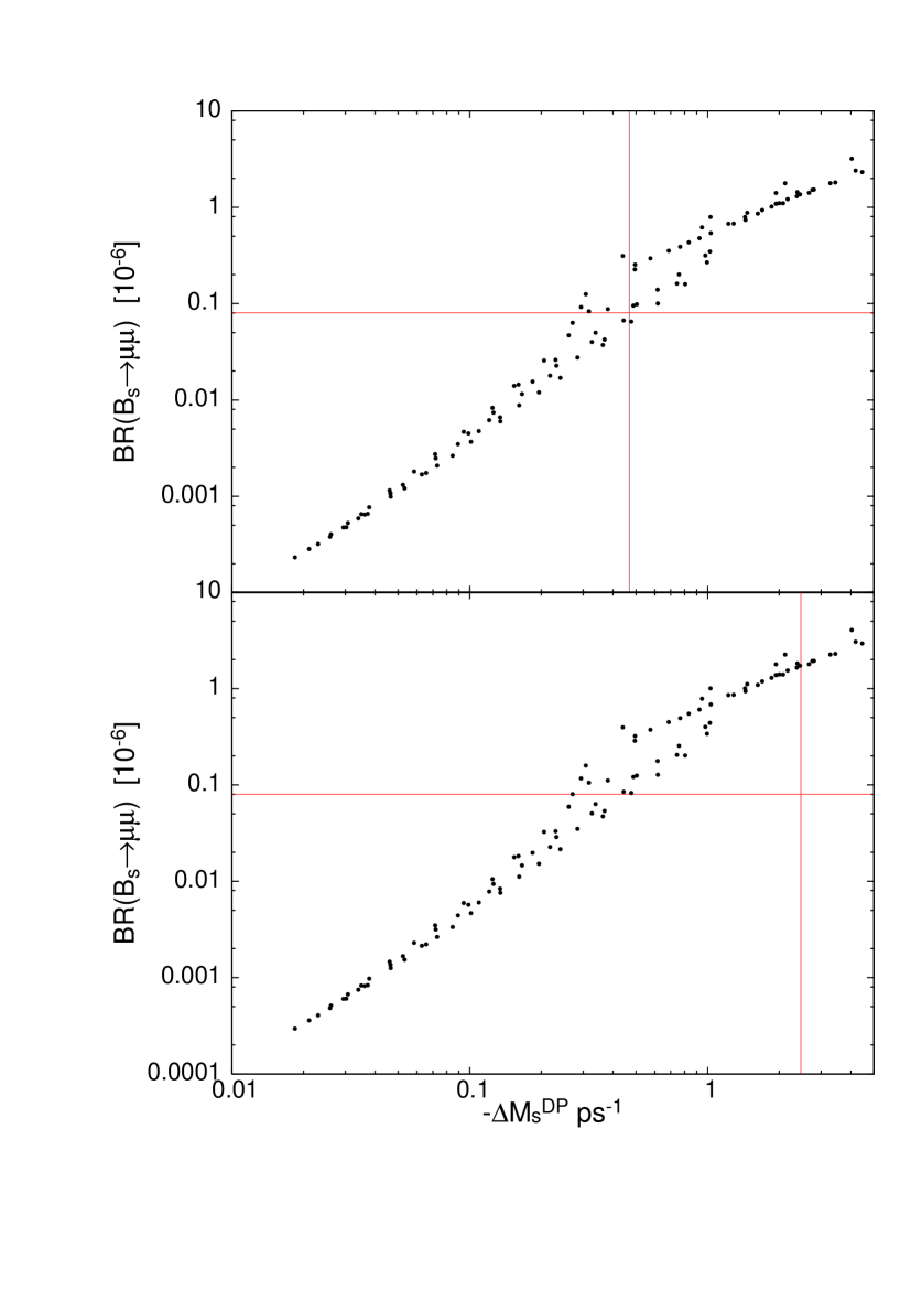
Figure 2: The correlation of Br$(B_{s}\to\mu^{+}\mu^{-})$ and $\Delta M_{s}^{DP}$ using $f_{B_{s}}=230$ MeV(upper panel) and $f_{B_{s}}=259$ MeV(lower panel). The horizontal and vertical lines show the present 90% C.L. upper bound[34] Br$(B_{s}\to\mu^{+}\mu^{-})<0.8\times 10^{-7}$ and the central value of the difference $(\Delta M_{s}^{CDF}\!\!-\!\Delta M_{s}^{SM})$ repectively.

Following the above conventions we can write the double penguin contribution to $\Delta M_{s}$ as,

$$\Delta M_{s}^{DP} \equiv 2{Re}\langle{\mathcal{H}}_{\sf eff}^{\Delta B=\Delta S=2}\rangle=\Delta M_{s}^{LL}+\Delta M_{s}^{LR}$$

$$= -\frac{1}{3}M_{B_{s}}f_{B_{s}}^{2}P_{1}^{SLL}\,\sum_{S}\,\frac{[X^{S}_{RL}]_{bs}[X^{S}_{RL}]_{bs}+[X^{S}_{LR}]_{bs}[X^{S}_{LR}]_{bs}}{M_{S}^{2}}$$

$$-\frac{2}{3}M_{B_{s}}f_{B_{s}}^{2}P_{2}^{LR}\,\sum_{S}\,\frac{[X^{S}_{RL}]_{bs}[X^{S}_{LR}]_{bs}}{M_{S}^{2}}$$

In eq. (1.1) we have defined $\Delta M_{s}^{LL}$ as the contribution from $Q^{SLL,SRR}_{1}$ and $\Delta M_{s}^{LR}$ from $Q^{LR}_{2}$. Here $P_{1}^{SLL}=-1.06$ and $P_{2}^{LR}=2.56$, include NLO QCD renormalisation group factors[35] and arise from the matrix elements of the operators of eq. (4). After taking into account the relative values of ${\mathcal{F}^{\pm}}$, the two $P$’s and the factor of 2 in eq. (1.1), we can see that there is a relative suppression,

$$\frac{\Delta M_{s}^{LL}}{\Delta M_{s}^{LR}}\approx\frac{\mathcal{F}^{-}}{\mathcal{F}^{+}}\cdot\frac{m_{b}}{m_{s}}\cdot\frac{P^{SLL}_{1}}{P^{LR}_{2}}\cdot\frac{1}{2}$$ (6)

This relative suppression shall be analysed further in the following section where it is shown that the contribution $\Delta M_{s}^{LL}$ is in fact significant.

Figure 3: Plot of the ratio, $\Delta M_{s}^{LL}/\Delta M_{s}^{LR}$, of the Higgs contributions from $Q_{1}^{SLL}$ and $Q_{2}^{LR}$.

There is a large non-perturbative uncertainty in the determination of $f_{B_{s}}$. Two recent lattice determinations provide [36, 37],

$$f_{B_{s}}^{{}^{\prime}04} = 230\pm 30\,{\rm MeV}$$ (7)

$$f_{B_{s}}^{{}^{\prime}05} = 259\pm 32\,{\rm MeV},$$ (8)

which in turn give different direct Standard Model predictions for $\Delta{M_{s}^{SM}}$,

$$\Delta M_{s}^{SM^{\prime}04} = 17.8\pm 8\,{\rm ps}^{-1}$$ (9)

$$\Delta M_{s}^{SM^{\prime}05} = 19.8\pm 5.5\,{\rm ps}^{-1}$$ (10)

The recent precise Tevatron measurement of $\Delta M_{s}$ is consistent with these direct SM prediction but with a lower central value [1, 2] ,

$$\Delta M_{s}^{CDF}=17.31^{+0.33}_{-0.18}\pm 0.07\,{\rm ps}^{-1}$$ (11)

2 Discussion

We shall now discuss the Higgs mediated contribution to $B_{s}$-$\bar{B}_{s}$ mixing, firstly in a simple SU(5) SUSY GUT and secondly for the MSSM Higgs sector using the FeynHiggs numerical package.

Figure 4: A plot of the relative suppression of $\Delta M_{s}^{LL}$ to $\Delta M_{s}^{LR}$ against the pseudoscalar Higgs mass. The plot is generated using the FeynHiggs package with the input values, $\tan\beta=50$, $\mu=1000$ GeV, $M_{SUSY}=500$ GeV and $X_{t}=1000$ GeV.

Recently a simple SUSY SU(5) model was studied using a top-down global $\chi^{2}$ analysis[22]. In this model the large $\tan\beta$ MSSM+$N_{R}$ is constrained at the GUT scale by SU(5) unification and universal soft SUSY breaking terms. In this work the best fits in the $(m_{0},\,M_{1/2})$ parameter space are used to make predictions for both $B_{s}\to\mu\mu$ and $\Delta M_{s}$.

In the limit of large $\tan\beta$, $B_{s}\to\mu^{+}\mu^{-}$ and $\Delta M_{s}$ are correlated. This correlation is shown in the two panels of fig. 2. For these two panels the two different values of $f_{B_{s}}$ listed in eq. (7,8) are used. The upper panel ($f_{B_{s}}=230$ MeV) shows that the central value of the difference $(\Delta M_{s}^{CDF}\!\!-\!\Delta M_{s}^{SM})$ coincides with the bound from Br$(B_{s}\to\mu^{+}\mu^{-})$. The lower panel ($f_{B_{s}}=259$ MeV) shows that the data points with $\Delta M_{s}^{DP}$ at the central value, are in fact ruled out by the bound on Br$(B_{s}\to\mu^{+}\mu^{-})$. The uncertainty in the SM prediction for $\Delta M_{s}$ is rather large and in fact all of the data points of fig. 2 are allowed by the recent Tevatron measurement at the $1\sigma$ level. These two panels clearly show that the interpretation of the recent measurement depends crucially on the uncertainty in the determination of $f_{B_{s}}$.

The plot in fig. 3 shows the ratio, $\Delta M_{s}^{LL}/\Delta M_{s}^{LR}$, of the contributions to the operators $Q_{1}^{SLL}$ and $Q_{2}^{LR}$ as defined in eq. (1.1). It is commonly assumed that the contribution to the $Q_{1}^{SLL}$ operator, $\Delta M_{s}^{LL}$, is negligible. From fig. 3 we can see that $\Delta M_{s}^{LL}$ is between 40% and 90% of $\Delta M_{s}^{LR}$ and hence is significant.

Figure 5: A plot of the relative suppression of $\Delta M_{s}^{LL}$ to $\Delta M_{s}^{LR}$ against $\mu$. The plot is generated using the FeynHiggs package with the input values, $\tan\beta=50$, $M_{A^{0}}=200$ GeV, $M_{SUSY}=500$ GeV and $X_{t}=1000$ GeV.

FeynHiggs[38, 39] is a numerical package for computing the MSSM Higgs boson masses and related observables, including higher-order corrections. Making use of this numerical package the relative suppression of $\Delta M_{s}^{LL}/\Delta M_{s}^{LR}$ for $\tan\beta=50$ was also studied. Using the FeynHiggs package the 2-loop corrected Higgs masses and CP even mixing parameter $\sin\alpha$ are used to calculate $\Delta M_{s}^{LL}/\Delta M_{s}^{LR}$ from the relation in eq. (6).

Figure 6: A plot of the relative suppression of $\Delta M_{s}^{LL}$ to $\Delta M_{s}^{LR}$ against $M_{SUSY}$. The plot is generated using the FeynHiggs package with the input values, $\tan\beta=50$, $M_{A^{0}}=500$ GeV, $\mu=1000$ GeV and $X_{t}=1000$ GeV.

The plot in fig. 4 shows the ratio of $\Delta M_{s}^{LL}/\Delta M_{s}^{LR}$ against the pseudoscalar Higgs mass. For this plot the values $\tan\beta=50$, $\mu=1000$ GeV, $M_{SUSY}=500$ GeV and $X_{t}\equiv(A_{t}-\mu\cot\beta)=1000$ GeV are used. The size of the suppression is similar to that seen in fig. 3. For light pseudoscalar Higgs mass the ratio is as large as 80%. For a pseudoscalar Higgs mass of 200 GeV the ratio is 45% and for a heavy mass the ratio remains at almost 20%. The same ratio is shown in fig. 5 plotted against the Higgs mass parameter $\mu$. Here the inputs are the same as fig. 4 with $M_{A^{0}}=200$ GeV and $\mu$ allowed to vary. In this case it is clear that the ratio $\Delta M_{s}^{LL}/\Delta M_{s}^{LR}$ increases with increasing $\mu$. Fig. 5 shows that for $\mu=1$ TeV the ratio is 45% and for $\mu=500$ GeV we still have a 10% effect. The plot in fig. 6 shows the variation of the relative suppression with the SUSY mass scale $M_{SUSY}$. Again this plot is generated using the same inputs as listed for fig. 4 with $M_{A^{0}}=200$ GeV and $M_{SUSY}$ allowed to vary. Here again we see that it is possible for a large contribution from $\Delta M_{s}^{LL}$ to exist particularly for light SUSY scales. For $M_{SUSY}=500$ GeV there is a 45% effect which remains at 10% for $M_{SUSY}=700$ GeV.

3 Conclusions

Using both a simple SUSY SU(5) model and the MSSM Higgs sector with the FeynHiggs numerical package, the Higgs mediated contribution to $\Delta M_{s}$ in the large $\tan\beta$ limit has been analysed. The constraint from the recent Tevatron measurement is found to be highly dependant upon the determination of $f_{B_{s}}$. It has been quite clearly shown however that there exists large regions of the MSSM parameter space for which the contribution from the operator $(\bar{b}P_{L}s)(\bar{b}P_{L}s)$ is non-negligible. The contribution to this operator may be as large as 80% of the dominant contribution via the operator $(\bar{b}P_{L}s)(\bar{b}P_{R}s)$. Therefore we find that this often ignored operator should be considered in any accurate determination of the MSSM contribution to the $B_{s}^{0}$-$\bar{B}_{s}^{0}$ mixing parameter $\Delta M_{s}$ in the large $\tan\beta$ regime.

References

- [1] A. Abulencia [CDF - Run II Collaboration], arXiv:hep-ex/0606027.
- [2] V. M. Abazov et al. [D0 Collaboration], Phys. Rev. Lett. 97 (2006) 021802
- [3] Z. Ligeti, M. Papucci and G. Perez, Phys. Rev. Lett. 97 (2006) 101801
- [4] P. Ball and R. Fleischer, arXiv:hep-ph/0604249.
- [5] Y. Grossman, Y. Nir and G. Raz, arXiv:hep-ph/0605028.
- [6] M. Ciuchini and L. Silvestrini, Phys. Rev. Lett. 97 (2006) 021803
- [7] M. Endo and S. Mishima, Phys. Lett. B 640 (2006) 205
- [8] J. Foster, K. i. Okumura and L. Roszkowski, arXiv:hep-ph/0604121.
- [9] S. Baek, arXiv:hep-ph/0605182.
- [10] R. Arnowitt, B. Dutta, B. Hu and S. Oh, arXiv:hep-ph/0606130.
- [11] M. Blanke, A. J. Buras, D. Guadagnoli and C. Tarantino, arXiv:hep-ph/0604057.
- [12] J. K. Parry, arXiv:hep-ph/0606150.
- [13] B. Dutta and Y. Mimura, arXiv:hep-ph/0607147.
- [14] K. Cheung, C. W. Chiang, N. G. Deshpande and J. Jiang, arXiv:hep-ph/0604223.
- [15] X. G. He and G. Valencia, Phys. Rev. D 74 (2006) 013011
- [16] S. Baek, J. H. Jeon and C. S. Kim, Phys. Lett. B 641 (2006) 183
- [17] S. Nandi and J. P. Saha, arXiv:hep-ph/0608341.
- [18] G. Xiangdong, C. S. Li and L. L. Yang, arXiv:hep-ph/0609269.
- [19] R. M. Wang, G. R. Lu, E. K. Wang and Y. D. Yang, arXiv:hep-ph/0609276.
- [20] L. X. Lu and Z. J. Xiao, arXiv:hep-ph/0609279.
- [21] S. Chang, C. S. Kim and J. Song, arXiv:hep-ph/0607313.
- [22] J. K. Parry, arXiv:hep-ph/0510305.
- [23] C. S. Huang, W. Liao and Q. S. Yan, Phys. Rev. D 59, 011701 (1999)
- [24] S. R. Choudhury and N. Gaur, Phys. Lett. B 451 (1999) 86
- [25] K. S. Babu and C. F. Kolda, Phys. Rev. Lett. 84, 228 (2000)
- [26] R. Hempfling, Phys. Rev. D49, 6168 (1994).
- [27] L. Hall, R. Rattazzi and U. Sarid, Phys. Rev. D50, 7048 (1994).
- [28] M. Carena, M. Olechowski, S. Pokorski and C. Wagner, Nucl. Phys. B426, 269 (1994).
- [29] T. Blazek, S. Raby and S. Pokorski, Phys. Rev. D 52, 4151 (1995)
- [30] C. Hamzaoui, M. Pospelov and M. Toharia, Phys. Rev. D 59, 095005 (1999)
- [31] T. Blazek, S. F. King and J. K. Parry, Phys. Lett. B 589 (2004) 39
- [32] A. J. Buras, P. H. Chankowski, J. Rosiek and L. Slawianowska, Nucl. Phys. B 659 (2003) 3
- [33] A. J. Buras, P. H. Chankowski, J. Rosiek and L. Slawianowska, Phys. Lett. B 546 (2002) 96
- [34] CDF collaboration, CDF Public Note 8176, www-cdf.fnal.gov
- [35] A. J. Buras, S. Jager and J. Urban, Nucl. Phys. B 605 (2001) 600
- [36] S. Hashimoto, Int. J. Mod. Phys. A 20 (2005) 5133
- [37] A. Gray et al. [HPQCD Collaboration], Phys. Rev. Lett. 95 (2005) 212001
- [38] T. Hahn, W. Hollik, S. Heinemeyer and G. Weiglein, arXiv:hep-ph/0507009.
- [39] S. Heinemeyer, W. Hollik and G. Weiglein, Comput. Phys. Commun. 124 (2000) 76