${\cal O}(\alpha_{s}^{2})$-corrections to JIMWLK evolution from the classical equations of motion

Abstract:

In this work we calculate some $\mathcal{O}(\alpha_{s}^{2})$ corrections to the JIMWLK kernel in the framework of the light-cone wave function approach to the high energy limit of QCD. The contributions that we consider originate from higher order corrections in the strong coupling and in the density of the projectile to the solution of the classical equations of motion that determine the Weizsäcker-Williams fields of the projectile. We study the structure of these corrections in the dipole limit, showing that they are subleading in the large-$N$ limit and that they cannot be fully recast in the form of dipole degrees of freedom, but rather present a complicated color structure.

1 Introduction

The contemporary description of the high energy evolution of QCD scattering amplitudes, given by the B-JIMWLK equations, has been developed over the last decade [1, 2, 3, 4, 5, 6, 7, 8, 9, 10, 11, 12, 13, 14, 15, 16, 17, 18, 19, 20] building upon the pioneering ideas on gluon saturation set out by Gribov, Levin and Ryskin [21] in the early 80s. Notwithstanding that the B-JIMWLK set of equations has proved difficult to tackle and that its complete solution remains unknown, a series of numerical [22, 23, 24, 25, 26, 27, 28, 29, 30] and analytical [31, 32, 33, 34, 35, 36] studies have established the asymptotic properties of the B-JIMWLK equations by considering their mean field limit, where the B-JIMWLK set reduces to a single closed equation — the Balitsky-Kovchegov (BK) equation [16, 17, 18, 37, 38]. Further, the results from this mean field equation deviate at most 10% from those obtained numerically from the full B-JIMWLK [30].

Significantly, the B-JIMWLK scheme neglects important effects [39, 40, 41, 42] — variably referred to as “Pomeron loops” [42, 43, 44, 45, 46, 47, 48, 49], “fluctuations” [41] or “wave function saturation effects” — due to gluon fluctuations. The insufficiencies of the B-JIMWLK framework become apparent once one recalls that these equations were derived under the explicit assumption — and, therefore, are strictly valid for such a physical situation — of large target gluon density and of a dilute projectile. Therefore, the B-JIMWLK formalism fails to properly describe the high-energy evolution for less asymmetrical systems (i.e. those where both target and projectile are dense). These crucial observations have led to a spurt of activity in this domain targeted at obtaining an evolution scheme correctly accounting for gluon fluctuation effects [40, 42, 43, 44, 45, 46, 47, 48, 49, 50, 51, 52, 53, 54, 55, 56, 57, 58]. A duality transformation linking the low and high density regimes [47, 48] places strict constraints on the form of any would-be complete evolution kernel.

Different paths have been followed in attempting to write an evolution kernel including dynamics beyond B-JIMWLK. A potentially fruitful path explores the connection between high energy QCD evolution and a reaction-diffusion process, [41] to suggest that the full dynamics should be described by an equation belonging to the universality class of the stochastic Fisher-Kolmogorov-Petrovsky-Piscunov (sFKPP) equation [42, 51, 52, 53, 45, 59]. A different strategy, the light-cone wave function approach [60, 47, 48, 49, 50], yields an evolution kernel not subject to the restrictions underlying the B-JIMWLK equations. This kernel, written in terms of the classical gluon fields of the projectile, reduces to the JIMWLK kernel when the fields are taken at leading order in the charge density. In this work we go one step further by computing the leading projectile density corrections.

This paper is organized as follows: in Sec. 2 we briefly introduce the light-cone wave function approach to high energy QCD. In Sec. 3 we present our general results for the leading projectile density correction, and in Sec. 4 we thoroughly discuss the dipole limit of the results of the previous section. Our conclusions are presented in Sec. 5.

2 Setup

We begin by reviewing the main features of the light-cone wave function approach to the high energy limit of QCD as derived by Kovner, Lublinsky and Wiedemann in [50, 60]. Consider the collision between a bunch of energetic gluons moving in the light-cone ‘+’ direction — the projectile — with a dense hadronic target characterized by large gluon fields. Let $Y$ be the total rapidity of the collision. The light-cone wave function of the incoming projectile is given by

$$|\Psi^{init}(Y)\rangle=\Psi[a_{i}^{a\dagger}(k^{+},\underline{k})]|0\rangle,$$ (1)

where $a^{a\dagger}_{i}(k^{+},\underline{k})$ are the creation operators for gluons with color index $a$, longitudinal momentum above some hard cutoff, $k^{+}\!\!>\!\!\Lambda^{+}$, and transverse momentum $\underline{k}$. Assuming that each of the gluons in the projectile interacts independently with the target, the wave function after the interaction is given by

$$|\Psi^{f}(Y)\rangle=\Psi[S^{ab}(x_{i})a_{i}^{b\dagger}]|0\rangle,$$ (2)

where $S^{ab}(x_{i})$ is the $S$-matrix corresponding to the propagation through the target of a single gluon located at transverse position $x_{i}$. At very high energies the interaction with the target eikonalizes and the $S$-matrix is diagonal in the transverse coordinates of the incoming gluons. Moreover, the $S$-matrix elements depend only on the gluon fields in the target, $A_{t}^{\mu}$, which allows us to take them, rather than the target fields themselves, as the physical degrees of freedom to describe the target. Although $S^{ab}$ is a quantum operator acting on the Hilbert space of the target fields, the commutators of $S$-operators are suppressed by powers of the target density, which hereinafter is assumed to be very large. Therefore $S^{ab}$ can, and will, be considered as a classical $c$-number, in the spirit of the semiclassical approach to dense gluonic systems [1, 2, 3]. With all this in mind, the scattering matrix of the projectile at rapidity $Y$ can be written as

$$\Sigma_{Y}[S]=\langle\Psi^{i}(Y)|\Psi^{f}(Y)\rangle.$$ (3)

High energy processes are characterized by a large separation of time scales — i.e. the time needed for the fast projectile to propagate through the target (the interaction time) is much shorter than the typical time scale under which the large, soft target fields vary. Thus, the fast projectile probes the target fields in a fixed, frozen configuration. Consequently, the physical scattering matrix is obtained by averaging over all the possible configurations of the gluon fields in the target:

$$\langle\Sigma\rangle=\int dS\,\Sigma[S]\,W_{Y}[S],$$ (4)

where the weight functional $W_{Y}[S]$ can be understood as the probability density for the target to have a certain configuration of the fields, $S$, at rapidity $Y$ (see [49] for a detailed discussion of the physical meaning and properties of $W_{Y}[S]$). In the wave function approach, the energy evolution of the system described above is achieved by boosting the projectile to higher rapidities, leaving the target unevolved. In this way all the information about the energy evolution of the system is encoded in the behavior of the projectile wave function as opposed to the strategy followed in the original derivation of the JIMWLK equation, in which the quantum fluctuations originated from boosting the target to higher energies were resummed in the presence of strong background fields, leading to the renormalization of the weight functional, $W_{Y}$.

To first order in $\delta Y$ the projectile wave function at rapidity $Y+\delta Y$ is given by:

$$|\Psi^{i}(Y+\delta Y)\rangle = \left\{1-\frac{1}{2}\delta Y\int d^{2}z\,b_{i}^{a}(z,[\rho])b_{i}^{a}(z,[\rho])\right.$$ (5)

$$+ \left.i\int d^{2}z\,b_{i}^{a}(z,[\rho])\int_{(1-\delta Y)\Lambda}^{\Lambda}\frac{dk^{+}}{\sqrt{\pi}|k^{+}|^{1/2}}\,a_{i}^{{}^{\dagger}a}(k^{+},z)\right\}|\Psi^{i}(Y)\rangle,$$

where $b_{i}$ are the Weizsäcker-Williams (WW) fields of the projectile, which depend uniquely on the projectile density operator $\rho$, defined as:

$$\rho^{a}=\,\int_{\Lambda^{+}}\!dk^{+}a_{i}^{\dagger b}(k^{+},z)T_{bc}^{a}\,a_{i}^{c}(k^{+},z),$$ (6)

where $T^{a}$ are the generators of $SU(N)$ in the adjoint representation. For a dilute projectile like the one considered here, the number of gluons in its wave function is small $\rho\sim\mathcal{O}(1)$. The physical meaning of Eq. (5) is clear: The hard, ‘valence’ gluons in the initial wave function are dressed with a cloud of soft gluons, the Weizsäcker-Williams (WW) fields $b_{i}$. These fields are determined from the classical Yang-Mills equations of motion (EOM), in which the hard gluons enter as an external source. The separation between soft and hard modes is made at an arbitrary scale $\Lambda^{+}$. The boost of the projectile opens up the phase space for the production of new hard gluons out of the soft WW fields. This production process is accounted for by the last term in the rhs of Eq. (5). The first term corresponds to no gluon production, whereas the second term corresponds to virtual corrections required to ensure the right normalization of the wave function.

The wave function of the projectile after the collision with the target is given by an analogous expression:

$$|\Psi^{f}(Y+\delta Y)\rangle = \left\{1-\frac{1}{2}\delta Y\int d^{2}z\,b_{i}^{a}(z,[S\rho])b_{i}^{a}(z,[S\rho])\right.$$

$$+ \left.i\int d^{2}z\,b_{i}^{a}(z,[S\rho])\int_{(1-\delta Y)\Lambda}^{\Lambda}\frac{dk^{+}}{\sqrt{\pi}|k^{+}|^{1/2}}S^{ab}(z)a_{i}^{{}^{\dagger}b}(k^{+},z)\right\}|\Psi^{f}(Y)\rangle,$$

where now the WW fields, $b_{i}$, are given by the solution of the classical EOM for rotated sources $S^{ab}\rho^{b}$. The scattering matrix of the evolved system is:

$$\Sigma[S](Y+\delta Y)=\langle\Psi^{i}(Y+\delta Y)|\Psi^{f}(Y+\delta Y)\rangle.$$ (8)

From Eq. (3) and Eq. (8), it is straightforward to derive an evolution equation for the scattering matrix $\Sigma[S]$ which, thanks to the Lorentz invariance of Eq. (4), can be converted into an evolution equation for the target weight functional, $W_{Y}$:

$${\delta W[S]\over\delta Y}=\chi\,W[S],$$ (9)

with the kernel of the evolution given by

$$\chi=-{1\over 2\pi}\int_{z}\,[b_{i}^{a}(z,[\rho])b_{i}^{a}(z,[\rho])+b_{i}^{a}(z,[S\rho])b_{i}^{a}(z,[S\rho])-2b_{i}^{b}(z,[\rho])b_{i}^{a}(z,[S\rho])S^{ba}(z)].$$ (10)

Importantly, Eq. (10) reduces to the JIMWLK kernel when the classical fields are taken at leading order in the charge density of the projectile, $g\rho$. Our goal is to derive higher order corrections to the JIMWLK evolution by solving the classical equations of motion at next order in $g\rho$.

At this point it should be noted that the expressions in Eq. (5) and Eq. (2) for the evolved wave function are not complete, and they are correct only in the limit of small projectile density. The more general expression for the evolved wave function as given by Eq. (2.5) in [49] includes an extra Bogolyubov transformation with respect to the expression in Eqs. (5) and (2) in this paper. It is argued in [49] and assumed in this work that such transformation reduces to the unity operator in the limit of small projectile density, $\rho\rightarrow 0$. Henceforth we restrict ourselves to the study of high density corrections to the kernel of the evolution arising from the expansion of the classical gluon fields, $b_{i}$, in terms of the projectile charge density, $g\rho$.

It is convenient to rewrite the kernel of the evolution in terms of left and right rotation operators, whose action on the scattering matrix of a gluonic projectile is defined as:

$$J_{L}^{a}(x)\,\Sigma[S] = -\mbox{tr}\left\{T^{a}S(x)\frac{\delta}{\delta S^{\dagger}(x)}\right\}\,\Sigma[S]\,,$$ (11)

$$J_{R}^{a}(x)\,\Sigma[S] = -\mbox{tr}\left\{S(x)T^{a}\frac{\delta}{\delta S^{\dagger}(x)}\right\}\,\Sigma[S]\,.$$ (12)

In terms of these operators, the kernel of the evolution reads

$$\chi=-\frac{1}{2\pi}\int_{z}\,[b_{i}^{a}(z,J_{L})b_{i}^{a}(z,J_{L})+b_{i}^{a}(z,J_{R})b_{i}^{a}(z,J_{R})-2b_{i}^{b}(z,[J_{L}])b_{i}^{a}(z,[J_{R}])S^{ba}(z)].$$ (13)

3 General results

To determine the WW fields entering the kernel of the evolution, Eq. (13), we need to solve the classical Yang-Mills equations of motion in the light-cone gauge, $A^{+}\!=\!0$, with the fast valence gluons playing the role of an external current. Since the hard gluons are fast moving in the ‘+’ direction, the current can be written as $J^{\nu}(z)=g\,\delta^{\nu+}\delta(z^{-})\rho(z)$, and the equations read

$$D_{\mu}F^{\mu\nu}(z)=J^{\nu}(z)\,,$$ (14)

$$D_{\mu}J^{\mu}(z)=0\,,$$ (15)

where Eq. (15) ensures the covariant conservation of the current. Since the number of gluons in the projectile is assumed to be small, $\sim\mathcal{O}(1)$, the current that they generate is of order $g$, $J\sim\mathcal{O}(g)$. Thus, $g$ will be the small parameter that controls our expansion of the solution.

The general solution of these equations has been extensively discussed in [61, 62]. In particular, it was shown in [1, 2, 3] that it is consistent to look for ‘static’ solutions of Eq. (14) — i.e, solutions independent of $x^{+}$, with $A^{-}=0$. Such a solution is a pure gauge with just transverse components. Under these assumptions Eq. (15) is trivially satisfied and, by writing the transverse components of the field as $A_{i}(z^{-},z)=\theta(z^{-})b_{i}(z)$, Eq. (14) becomes

$$\partial_{i}b^{a}_{i}(z)+gf^{abc}\,b_{i}^{b}(z)b_{i}^{c}(z)=g\rho^{a}(z)\,,$$ (16)

$$\partial_{i}b^{a}_{j}(z)-\partial_{j}b^{a}_{i}(z)+gf^{abc}\,b_{i}^{b}(z)b_{j}^{c}(z)=0\,,$$ (17)

Expanding the solutions in powers of $g$:

$$b^{a}_{i}(z)=g\left(b^{a}_{i1}(z)+g^{2}\,b^{a}_{i2}(z)+\mathcal{O}(g^{4})\right),$$ (18)

we get

$$b^{a}_{i1}(z)=\frac{1}{2\pi}\int d^{2}x\frac{(z-x)_{i}}{(z-x)^{2}}\,\rho^{a}(z)=\frac{1}{2\pi}\int\!d^{2}x\,\left(\partial_{i}X\right)\rho^{a}(z),$$ (19)

$$b^{a}_{i2}(z)=-\frac{1}{4(2\pi)^{2}}f^{abc}\!\int d^{2}x\,d^{2}y\,(X\!\stackrel{{\scriptstyle\leftrightarrow}}{{\partial_{i}}}\!Y)\rho^{b}(x)\rho^{c}(y),$$ (20)

where we have made use of the following shorthand notation for the coordinate dependence of the solution:

$$\partial_{i}X\equiv\partial^{z}_{i}\ln\left(|z-x|\lambda\right)\,,$$

$$X\!\stackrel{{\scriptstyle\leftrightarrow}}{{\partial_{i}}}\!Y\equiv X\left(\partial^{z}_{i}Y\right)-\left(\partial^{z}_{i}X\right)Y\,,$$ (21)

where $\partial^{z}_{i}$ denotes the partial derivative with respect to the transverse components of $z$, $i=1,2$.

The expansion of the solution in Eq. (18) immediately translates into an expansion for the kernel of the evolution in powers of $\alpha_{s}=g^{2}/4\pi$:

$$\chi=\alpha_{s}\left(\chi^{1)}+\alpha_{s}\,\chi^{2)}+\mathcal{O}(\alpha_{s}^{2})\right),$$ (22)

whose leading term is the JIMWLK kernel:

$$\alpha_{s}\chi^{1)}=\chi^{JIMWLK} = -\frac{\alpha_{s}}{2\pi^{2}}\int_{xyz}\!\!(\partial_{i}X)(\partial_{i}Y)\left[J_{L}^{a}(z)J_{L}^{a}(z)\right.$$ (23)

$$+\left.J_{R}^{a}(z)J_{R}^{a}(z)-2J_{L}^{a}(z)J_{R}^{b}(z)S^{ab}(z)\right].$$

The first correction to JIMWLK, $\chi^{2)}$, is obtained by keeping terms up to order $\alpha_{s}^{2}$ in the product WW fields, yielding

$$\chi^{2)} = -\frac{1}{(2\pi)^{2}}\int_{xywz}f^{abc}\,(\partial_{i}Y)(X\!\stackrel{{\scriptstyle\leftrightarrow}}{{\partial_{i}}}\!W)\,\left[J_{L}^{a}(x)J_{L}^{b}(y)J_{L}^{c}(w)+J_{R}^{a}(x)J_{R}^{b}(y)J_{R}^{c}(w)\right]$$ (24)

$$-2f^{acd}(\partial_{i}X)(Y\!\stackrel{{\scriptstyle\leftrightarrow}}{{\partial_{i}}}\!W)S^{ba}(z)\left[J_{L}^{b}(x)J_{R}^{c}(y)J_{R}^{d}(w)+J_{L}^{b}(x)J_{L}^{c}(y)J_{R}^{d}(w)\right].$$

Note that from the second order solution of the EOM we could immediately derive part of the $\mathcal{O}(\alpha_{s}^{3})$ corrections to the kernel. However, a complete derivation of the $\mathcal{O}(\alpha_{s}^{3})$ term in Eq. (22) would require the $O(g^{5})$ solution to the EOM, which is beyond the scope of this paper.

4 Dipole model limit

The color structure of a generic projectile composed of gluons can be rather complicated, consisting of different color multipoles mix with each other through the evolution in a highly non-trivial way. However, in the large-$N$ limit this complicated structure is greatly simplified and the high energy evolution can be recast in terms of dipole degrees of freedom. More precisely, the JIMWLK equation is equivalent to an infinite hierarchy of coupled differential equations for the correlators of the gluon fields. In the large-$N$ limit the whole hierarchy decouples and one is left with a single, closed, non-linear evolution equation for the dipole scattering amplitude — the BK equation [16, 17, 18, 37, 38].

In this section we explore the color structure of the correction to JIMWLK evolution derived in the previous section. In order to do so, we consider an initial projectile entirely describable by dipole degrees of freedom:

$$\Sigma=\Sigma[s],$$ (25)

where

$$s(x,y)=\frac{1}{N}\mbox{tr}\{S_{F}^{\dagger}(y)S_{F}(x)\}$$ (26)

is the scattering matrix for a $q$-$\bar{q}$ dipole, with $x$ and $y$ the transverse coordinates of, respectively, the quark and the antiquark. The subscript $F$ in the rhs of Eq. (26) indicates that the scattering matrix is to be taken for particles in the fundamental representation of $SU(N)$, and will be usually omitted in the following. Our purpose is to study the resulting color structure of the projectile under evolution, i.e. we want to calculate $\chi^{2)}\,\Sigma[s]$. The action of the left and right rotation operators on a dipole-like projectile scattering matrix is given by:

$$J_{L}^{a}(x)\,s[u,v] = -\frac{1}{2}\,\mbox{tr}\left\{t^{a}S(x)\frac{\delta}{\delta S^{T}(x)}-S^{\dagger}(x)t^{a}\frac{\delta}{\delta S^{*}(x)}\right\}\,s[u,v]\,,$$ (27)

$$J_{R}^{a}(x)\,s[u,v] = -\frac{1}{2}\,\mbox{tr}\left\{S(x)t^{a}\frac{\delta}{\delta S^{T}(x)}-t^{a}S^{\dagger}(x)\frac{\delta}{\delta S^{*}(x)}\right\}\,s[u,v]\,,$$ (28)

where $t^{a}$ are now the $SU(N)$ generators in the fundamental representation. From Eqs. (27) and (28) it can be proved that both $J_{L}$ and $J_{R}$ are hermitian operators, a property which immediately ensures the hermiticity of the kernel of the evolution.

4.1 General expressions

Using the following notation for the functional derivatives of the scattering matrix:

$$\delta_{uv;\dots;qt}\Sigma\equiv\left[\frac{\delta}{\delta s(u,v)}\cdots\frac{\delta}{\delta s(q,t)}\right]\,\Sigma[s],$$ (29)

and defining $S_{z}\equiv S_{F}(z)$, we can write the action of the different pieces of the kernel in Eq. (24) on $\Sigma[s]$ as

$$f^{abc} \!\!\!\!J_{R}^{a}(x)J_{R}^{b}(y)J_{R}^{c}(w)\Sigma[s]=-\frac{1}{N}f^{abc}[\delta(\!v\!-\!w\!)\!-\!\delta(\!u\!-\!w\!)]\Bigl{.}\Bigr{\{}$$

$$\qquad[\delta(\!v\!-\!y\!)\!+\!\delta(\!u\!-\!y\!)][\delta(\!v\!-\!x\!)\!-\!\delta(\!u\!-\!x\!)]\mbox{tr}\{S^{\dagger}_{u}S_{v}t^{a}t^{b}t^{c}\}\delta_{uv}\Sigma$$

$$+\frac{1}{N}[\delta(\!v\!-\!y\!)\!+\!\delta(\!u\!-\!y\!)][\delta(\!r\!-\!x\!)\!-\!\delta(\!p\!-\!x\!)]\mbox{tr}\{S^{\dagger}_{u}S_{v}t^{b}t^{c}\}\mbox{tr}\{S^{\dagger}_{p}S_{r}t^{a}\}\delta_{pr;uv}\Sigma$$

$$+\frac{1}{N}[\delta(\!r\!-\!y\!)\!-\!\delta(\!p\!-\!y\!)][\delta(\!v\!-\!x\!)\!+\!\delta(\!u\!-\!x\!)]\mbox{tr}\{S^{\dagger}_{u}S_{v}t^{a}t^{c}\}\mbox{tr}\{S^{\dagger}_{p}S_{r}t^{b}\}\delta_{pr;uv}\Sigma$$

$$+\frac{1}{N}[\delta(\!r\!-\!y\!)\!-\!\delta(\!p\!-\!y\!)][\delta(\!r\!-\!x\!)\!+\!\delta(\!p\!-\!x\!)]\mbox{tr}\{S^{\dagger}_{u}S_{v}t^{c}\}\mbox{tr}\{S^{\dagger}_{p}S_{r}t^{a}t^{b}\}\delta_{pr;uv}\Sigma$$

$$\left.+\frac{1}{N^{2}}[\delta(\!r\!-\!y\!)\!-\!\delta(\!p\!-\!y\!)][\delta(\!t\!-\!x\!)\!-\!\delta(\!q\!-\!x\!)]\mbox{tr}\{S^{\dagger}_{u}S_{v}t^{c}\}\mbox{tr}\{S^{\dagger}_{p}S_{r}t^{b}\}\mbox{tr}\{S^{\dagger}_{q}S_{t}t^{a}\}\delta_{qt;pr;uv}\Sigma\right\},$$

$$f^{abc} \!\!\!\!J_{L}^{a}(x)J_{L}^{b}(y)J_{L}^{c}(w)\Sigma[s]=-\frac{1}{N}f^{abc}[\delta(\!v\!-\!w\!)\!-\!\delta(\!u\!-\!w\!)]\Bigl{.}\Bigr{\{}\hskip 28.45274pt$$

$$\qquad[\delta(\!v\!-\!y\!)\!+\!\delta(\!u\!-\!y\!)][\delta(\!v\!-\!x\!)\!-\!\delta(\!u\!-\!x\!)]\mbox{tr}\{S^{\dagger}_{u}t^{c}t^{b}t^{a}S_{v}\}\delta_{uv}\Sigma$$

$$+\frac{1}{N}[\delta(\!v\!-\!y\!)\!+\!\delta(\!u\!-\!y\!)][\delta(\!r\!-\!x\!)\!-\!\delta(\!p\!-\!x\!)]\mbox{tr}\{S^{\dagger}_{u}t^{c}t^{b}S_{v}\}\mbox{tr}\{S^{\dagger}_{p}t^{a}S_{r}\}\delta_{pr;uv}\Sigma$$

$$+\frac{1}{N}[\delta(\!r\!-\!y\!)\!-\!\delta(\!p\!-\!y\!)][\delta(\!v\!-\!x\!)\!+\!\delta(\!u\!-\!x\!)]\mbox{tr}\{S^{\dagger}_{u}t^{c}t^{a}S_{v}\}\mbox{tr}\{S^{\dagger}_{p}t^{b}S_{r}\}\delta_{pr;uv}\Sigma$$

$$+\frac{1}{N}[\delta(\!r\!-\!y\!)\!-\!\delta(\!p\!-\!y\!)][\delta(\!r\!-\!x\!)\!+\!\delta(\!p\!-\!x\!)]\mbox{tr}\{S^{\dagger}_{u}t^{c}S_{v}\}\mbox{tr}\{S^{\dagger}_{p}t^{b}t^{a}S_{r}\}\delta_{pr;uv}\Sigma$$

$$\left.+\frac{1}{N^{2}}[\delta(\!r\!-\!y\!)\!-\!\delta(\!p\!-\!y\!)][\delta(\!t\!-\!x\!)\!-\!\delta(\!q\!-\!x\!)]\mbox{tr}\{S^{\dagger}_{u}t^{c}S_{v}\}\mbox{tr}\{S^{\dagger}_{p}t^{b}S_{r}\}\mbox{tr}\{S^{\dagger}_{q}t^{a}S_{t}\}\delta_{qt;pr;uv}\Sigma\right\},$$

$$f^{acd} \!\!\!\!J_{L}^{b}(x)J_{R}^{c}(y)J_{R}^{d}(w)\Sigma[s]=-\frac{1}{N}f^{acd}[\delta(\!v\!-\!w\!)\!-\!\delta(\!u\!-\!w\!)]\Bigl{.}\Bigr{\{}\hskip 28.45274pt$$

$$\qquad[\delta(\!v\!-\!y\!)\!+\!\delta(\!u\!-\!y\!)][\delta(\!v\!-\!x\!)\!-\!\delta(\!u\!-\!x\!)]\mbox{tr}\{S^{\dagger}_{u}t^{b}S_{v}t^{c}t^{d}\}\delta_{uv}\Sigma$$

$$+\frac{1}{N}[\delta(\!v\!-\!y\!)\!+\!\delta(\!u\!-\!y\!)][\delta(\!r\!-\!x\!)\!-\!\delta(\!p\!-\!x\!)]\mbox{tr}\{S^{\dagger}_{u}S_{v}t^{c}t^{d}\}\mbox{tr}\{S^{\dagger}_{p}t^{b}S_{r}\}\delta_{pr;uv}\Sigma$$

$$+\frac{1}{N}[\delta(\!r\!-\!y\!)\!-\!\delta(\!p\!-\!y\!)][\delta(\!v\!-\!x\!)\!-\!\delta(\!u\!-\!x\!)]\mbox{tr}\{S^{\dagger}_{u}t^{b}\S_{v}t^{d}\}\mbox{tr}\{S^{\dagger}_{p}S_{r}t^{c}\}\delta_{pr;uv}\Sigma$$

$$+\frac{1}{N}[\delta(\!r\!-\!y\!)\!-\!\delta(\!p\!-\!y\!)][\delta(\!r\!-\!x\!)\!-\!\delta(\!p\!-\!x\!)]\mbox{tr}\{S^{\dagger}_{u}S_{v}t^{d}\}\mbox{tr}\{S^{\dagger}_{p}t^{b}S_{r}t^{c}\}\delta_{pr;uv}\Sigma$$

$$\left.+\frac{1}{N^{2}}[\delta(\!r\!-\!y\!)\!-\!\delta(\!p\!-\!y\!)][\delta(\!t\!-\!x\!)\!-\!\delta(\!q\!-\!x\!)]\mbox{tr}\{S^{\dagger}_{u}S_{v}t^{d}\}\mbox{tr}\{S^{\dagger}_{p}S_{r}t^{c}\}\mbox{tr}\{S^{\dagger}_{q}t^{b}S_{t}\}\delta_{qt;pr;uv}\Sigma\right\},$$

and

$$f^{bcd} \!\!\!\!J_{L}^{c}(w)J_{L}^{d}(y)J_{R}^{a}(x)\Sigma[s]=-\frac{1}{N}f^{bdc}[\delta(\!v\!-\!x\!)\!-\!\delta(\!u\!-\!x\!)]\Bigl{.}\Bigr{\{}\hskip 28.45274pt$$

$$\qquad[\delta(\!v\!-\!w\!)\!-\!\delta(\!u\!-\!w\!)][\delta(\!v\!-\!y\!)\!+\!\delta(\!u\!-\!y\!)]\mbox{tr}\{S^{\dagger}_{u}t^{d}t^{c}S_{v}t^{a}\}\delta_{uv}\Sigma$$

$$+\frac{1}{N}[\delta(\!v\!-\!w\!)\!-\!\delta(\!u\!-\!w\!)][\delta(\!r\!-\!y\!)\!-\!\delta(\!p\!-\!y\!)]\mbox{tr}\{S^{\dagger}_{u}t^{d}S_{v}t^{a}\}\mbox{tr}\{S^{\dagger}_{p}t^{c}S_{r}\}\delta_{pr;uv}\Sigma$$

$$+\frac{1}{N}[\delta(\!r\!-\!w\!)\!-\!\delta(\!p\!-\!w\!)][\delta(\!v\!-\!y\!)\!-\!\delta(\!u\!-\!y\!)]\mbox{tr}\{S^{\dagger}_{u}t^{c}S_{v}t^{a}\}\mbox{tr}\{S^{\dagger}_{p}t^{d}S_{r}\}\delta_{pr;uv}\Sigma$$

$$+\frac{1}{N}[\delta(\!r\!-\!w\!)\!-\!\delta(\!p\!-\!w\!)][\delta(\!r\!-\!y\!)\!+\!\delta(\!p\!-\!y\!)]\mbox{tr}\{S^{\dagger}_{u}S_{v}t^{a}\}\mbox{tr}\{S^{\dagger}_{p}t^{d}t^{c}S_{r}\}\delta_{pr;uv}\Sigma$$

$$\left.+\frac{1}{N^{2}}[\delta(\!r\!-\!w\!)\!-\!\delta(\!p\!-\!w\!)][\delta(\!t\!-\!y\!)\!-\!\delta(\!q\!-\!y\!)]\mbox{tr}\{S^{\dagger}_{u}S_{v}t^{a}\}\mbox{tr}\{S^{\dagger}_{p}t^{d}S_{r}\}\mbox{tr}\{S^{\dagger}_{q}t^{c}S_{t}\}\delta_{qt;pr;uv}\Sigma\right\}.$$

4.2 Diagrammatic interpretation

Despite the fact that the expressions derived in the previous section appear complicated, they allow for a very clear physical interpretation in terms of diagrams according to the following rules: the action of the left (right) rotation operator, $J_{L(R)}^{a}$, on the projectile scattering matrix brings in a new dipole, along with the the corresponding $1/N$ suppression factor, which emits a new gluon of color $a$ before (or after) the interaction with the target. Such emission may happen either from the quark line or from the antiquark. In the former case a, relative minus sign is picked up. Subsequent actions of the rotation operators may act either on $\Sigma[s]$, bringing new dipoles into the diagram, or on the preexisting dipole, which emits a new gluon. These rules are sketched in Fig. 1.

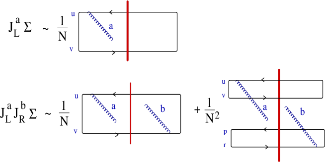
Figure 1: Diagrammatic representation of $J_{L}^{a}\Sigma$ (top) and $J_{L}^{a}J_{R}^{b}\Sigma$ (bottom). The target is represented by the vertical thick line.

In order to fully describe the diagrams in terms of fundamental constituents, quark and antiquark lines, we make use of the Fierz identity:

$$(t^{a})_{ij}(t^{b})_{kl}=\frac{1}{2}(\delta_{il}\delta_{jk}-\frac{1}{N}\delta_{ij}\delta_{kl}),$$ (34)

which can be translated into diagrammatic language substituting the gluon lines by quark-antiquark lines as indicated in Fig. 2.

Figure 2: Pictorial representation of the Fierz identity Eq. (34).

The propagation of each quark (antiquark) line through the target at transverse coordinate $x$ is accounted for the scattering matrix, $S_{F}(x)$ ($S_{F}^{\dagger}(x)$). Finally, the trace over closed fermion lines has to be taken. Following these rules, it is straightforward to rederive the results in Eqs. (4.1)-(4.1). As an example, we show in Fig. 3 the diagrams corresponding to the action of $J_{L}J_{L}J_{L}\Sigma[s]$, Eq. (4.1), and $J_{L}J_{L}J_{R}\Sigma[s]$, Eq. (4.1), in which, for the sake of simplicity, we have kept the gluon lines in the adjoint representation without using the Fierz identity.

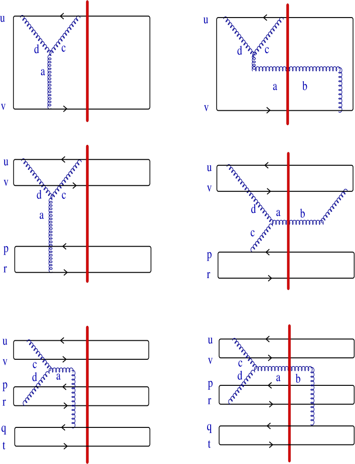
Figure 3: Diagrams corresponding to the LLL (plots on the left) and LLR (plots on the right), see the accompanying text. The diagrams include one ($\propto 1/N$, top), two ($\propto 1/N^{2}$, middle) and three ($\propto 1/N^{3}$, bottom) active dipoles. The thick vertical line represents the target.

4.3 Symmetry considerations

Before proceeding further it is convenient to divide our final result into three pieces according to their leading power of $1/N$ as given by the number of dipoles appearing in the relevant diagram, see the previous subsection:

$$\chi^{2)}\Sigma[s]=\left(\chi^{2)}_{1/N}+\chi^{2)}_{1/N^{2}}+\chi^{2)}_{1/N^{3}}\right)\Sigma[s].$$ (35)

To complete the calculation we still have to plug in the results from Eqs. (4.1)-(4.1). into Eq. (24), perform the contraction of the color indices and integrate over $x,y,w$. Further, the cross terms LRR, Eq. (4.1), and LLR, Eq. (4.1), must be contracted with the scattering matrix for a single gluon, $S_{A}^{ab}$, which can be rewritten in terms of matrices in the fundamental representation by means of the Fierz identity:

$$S_{A}^{ab}(z)=2\,\mbox{tr}\{S_{F}^{\dagger}(z)t^{b}S_{F}(z)t^{a}\}.$$ (36)

The $SU(N)$ algebra can be worked out using the relations listed in the Appendix.

After all this is done, we note that the contribution to the kernel coming from the pieces of order $1/N$ in Eqs. (4.1) and (4.1) cancel each other out. An analogous cancellation happens between the leading $1/N$ contributions from Eqs. (4.1) and (4.1). Therefore

$$\chi^{2)}_{1/N}\Sigma[s]=0.$$ (37)

It is clear from the diagrammatic rules derived in 4.2 that this cancellation corresponds to the diagrams in which all the emissions and absorptions of gluons happen in a single dipole, while the other dipoles in the wave function remain as spectators. More precisely, the top diagrams in Fig. 3 cancel against their respective complex conjugate diagrams (not shown in the figure).

An analogous cancellation occurs for the $1/N^{2}$ terms in Eqs. (4.1) and (4.1). Diagrammatically, the middle-left diagram in Fig. 3 cancels against its complex conjugate. Therefore, the leading $1/N^{2}$ contribution is given by the $1/N^{2}$ terms in Eqs. (4.1) and (4.1) (middle-right diagram in Fig. 3 plus its complex conjugate). We get

$$\chi^{2)}_{1/N^{2}}\Sigma[s]=\frac{i}{(2\pi)^{2}}\frac{1}{N^{2}}\Biggl{\{}\int d^{2}z\\ -N[\partial_{i}(R\!-\!P)][U\stackrel{{\scriptstyle\leftrightarrow}}{{\partial_{i}}}V][\mbox{tr}\{S^{\dagger}_{u}S_{v}S^{\dagger}_{z}S_{r}S^{\dagger}_{p}S_{z}\}-\frac{1}{N}\mbox{tr}\{S^{\dagger}_{u}S_{v}\}\mbox{tr}\{S^{\dagger}_{p}S_{r}\}]\\ -\frac{1}{2}\,[\partial_{i}(V\!-\!U)][(R\!-\!P)\stackrel{{\scriptstyle\leftrightarrow}}{{\partial_{i}}}(V\!-\!U)][\mbox{tr}\{S^{\dagger}_{z}S_{v}S^{\dagger}_{p}S_{r}\}\mbox{tr}\{S^{\dagger}_{u}S_{z}\}-\mbox{tr}\{S^{\dagger}_{u}S_{z}S^{\dagger}_{p}S_{r}\}\mbox{tr}\{S^{\dagger}_{z}S_{v}\}]\\ +\frac{1}{2}\,[\partial_{i}(R\!-\!P)][(R\!-\!P)\stackrel{{\scriptstyle\leftrightarrow}}{{\partial_{i}}}(V\!-\!U)][\mbox{tr}\{S^{\dagger}_{z}S_{r}S^{\dagger}_{u}S_{v}\}\mbox{tr}\{S^{\dagger}_{p}S_{z}\}-\mbox{tr}\{S^{\dagger}_{p}S_{z}S^{\dagger}_{u}S_{v}\}\mbox{tr}\{S^{\dagger}_{z}S_{r}\}]\\ -\frac{1}{2}\,[\partial_{i}(V\!-\!U)][(R\!-\!P)\stackrel{{\scriptstyle\leftrightarrow}}{{\partial_{i}}}(V\!-\!U)][\mbox{tr}\{S_{z}S^{\dagger}_{u}S_{r}S^{\dagger}_{p}\}\mbox{tr}\{S^{\dagger}_{z}S_{v}\}-\mbox{tr}\{S^{\dagger}_{p}S_{v}S^{\dagger}_{z}S_{r}\}\mbox{tr}\{S^{\dagger}_{u}S_{z}\}]\\ +\frac{1}{2}\,[\partial_{i}(V\!-\!U)][(V\!-\!U)\stackrel{{\scriptstyle\leftrightarrow}}{{\partial_{i}}}(R\!-\!P)][\mbox{tr}\{S_{z}S^{\dagger}_{u}S_{r}S^{\dagger}_{p}\}\mbox{tr}\{S^{\dagger}_{z}S_{v}\}-\mbox{tr}\{S^{\dagger}_{p}S_{v}S^{\dagger}_{z}S_{r}\}\mbox{tr}\{S^{\dagger}_{u}S_{z}\}]\\ +{N}[\partial_{i}(V\!-\!U)][P\stackrel{{\scriptstyle\leftrightarrow}}{{\partial_{i}}}R][\mbox{tr}\{S^{\dagger}_{u}S_{v}S^{\dagger}_{z}S_{r}S^{\dagger}_{p}S_{z}\}-\frac{1}{N}\mbox{tr}\{S^{\dagger}_{u}S_{v}\}\mbox{tr}\{S^{\dagger}_{p}S_{r}\}]\Biggr{\}}\,\frac{\delta^{2}\Sigma[s]}{\delta s(p,r)\delta s(u,v)}\,.$$ (38)

This result can be further simplified by noting that any wave function or weight functional of a gluonic/dipole configuration has to be completely symmetric under the exchange of any number of gluons/dipoles, such that the exchange $(u,v)\leftrightarrow(p,r)$ leaves the action of the functional derivative $\delta_{uv;pr}\Sigma$ unchanged. Under such an exchange, many terms in Eq. (38) cancel each other, yielding:

$$\chi^{2)}_{1/N^{2}}\Sigma[s]=-\frac{i}{(2\pi)^{2}}\,\frac{1}{N^{2}}\int d^{2}z\,\Big{\{}$$

$$[\partial_{i}(R\!-\!P)(U\!\stackrel{{\scriptstyle\leftrightarrow}}{{\partial_{i}}}\!V)-\partial(V\!-\!U)(P\!\stackrel{{\scriptstyle\leftrightarrow}}{{\partial_{i}}}\!R)][N\,\mbox{tr}\{S_{u}^{\dagger}S_{v}S_{z}^{\dagger}S_{r}S_{p}^{\dagger}S_{z}\}]$$

$$+\partial_{i}(V\!-\!U)(R\!-\!P)\stackrel{{\scriptstyle\leftrightarrow}}{{\partial_{i}}}(V\!-\!U)\left[\mbox{tr}\{S_{z}^{\dagger}S_{v}S_{p}^{\dagger}S_{r}\}\mbox{tr}\{S_{u}^{\dagger}S_{z}\}-\mbox{tr}\{S_{u}^{\dagger}S_{z}S_{p}^{\dagger}S_{r}\}\mbox{tr}\{S_{z}^{\dagger}S_{v}\}\right.$$

$$\left.+\mbox{tr}\{S_{p}^{\dagger}S_{z}S_{u}^{\dagger}S_{r}\}\mbox{tr}\{S_{z}^{\dagger}S_{v}\}-\mbox{tr}\{S_{p}^{\dagger}S_{v}S_{z}^{\dagger}S_{r}\}\mbox{tr}\{S_{u}^{\dagger}S_{z}\}\right]\Big{\}}\,\frac{\delta^{2}\Sigma[s]}{\delta s(p,r)\delta s(u,v)}\,\,.$$ (39)

Calculating the $1/N^{3}$ terms in an analogous way we get:

$$\chi^{2)}_{1/N^{3}}\Sigma[s]=-\frac{i}{2}\,\frac{1}{(2\pi)^{2}}\,\frac{1}{N^{3}}\int d^{2}z\left[\{\partial_{i}(R\!-\!P)\}\{(T\!-\!Q)\stackrel{{\scriptstyle\leftrightarrow}}{{\partial_{i}}}(V\!-\!U)\}\right]$$

$$\times\left[\mbox{tr}\{S^{\dagger}_{u}S_{v}S^{\dagger}_{q}S_{t}S^{\dagger}_{p}S_{r}\}+\mbox{tr}\{S^{\dagger}_{u}S_{t}S^{\dagger}_{q}S_{r}S^{\dagger}_{p}S_{v}\}+\mbox{tr}\{S^{\dagger}_{z}S_{r}S^{\dagger}_{p}S_{z}S^{\dagger}_{u}S_{v}S^{\dagger}_{q}S_{t}\}\right.$$

$$\left.+\mbox{tr}\{S^{\dagger}_{p}S_{r}S^{\dagger}_{z}S_{v}S^{\dagger}_{u}S_{t}S^{\dagger}_{q}S_{z}\}\right]\frac{\delta^{3}\Sigma[s]}{\delta s(q,t)\delta s(p,r)\delta s(u,v)}\,\,.$$ (40)

Eqs. (37), (39) and (40) are the central result of this paper. One of their main features is the fact that the action of the kernel on a dipole-like projectile cannot be entirely recast in terms of dipole degrees of freedom. On the contrary, the evolution generates a complicated color structure consisting in the mixing of dipoles, quadrupoles, sextupoles and octupoles as given by these equations, which can only be expressed partially as dipole degrees of freedom by increasing the power in $1/N$. Consequently, these corrections to the leading JIMWLK kernel bring no corrections to the mean field BK equation.

5 Conclusions

In this work we have calculated the $\mathcal{O}(\alpha_{s}^{2})$ corrections to the JIMWLK kernel that arise from the $\mathcal{O}(g^{3})$ solutions to the classical Yang-Mills equations. These are the first corrections in the charge density of the projectile to JIMWLK evolution, and therefore partially account for the coherence effects in the projectile gluon emission which drives small-$x$ evolution. In the context of the present discussions on the quest for evolution equations for scattering of a dense projectile which would contain the so-called pomeron loops, our result accounts for the part of these corrections not arising from the non-commutativity of the target fields. Thus, they are restricted to the dilute-dense scattering situation. The same systematic technique could be used to improve the results, although admittedly the computation of even higher orders looks technically challenging.

Our main result is the cancellation of the leading $1/N$ contributions, together with Eqs. (39)-(40). We provide a diagrammatic interpretation of these results. These corrections are subleading in $1/N$ and exhibit a complicated color structure. They do not, therefore, provide any correction to the BK equation but, rather, add new terms to the Balitsky hierarchy.

Appendix A Some color algebra

In this appendix we list some relations needed to derive the results in section 4. Using the basic $SU(N)$ relations

$$f^{ade}f^{bef}f^{cfd}=\frac{N}{2}f^{abc}\,,$$ (41)

$$d^{ade}d^{bef}f^{cfd}=\left(\frac{2}{N}-\frac{N}{2}\right)f^{abc}\,,$$ (42)

$$d^{ade}f^{bef}f^{cfd}=-\frac{N}{2}\,d^{abc}\,,$$ (43)

$$d^{ade}d^{bef}d^{cfd}={N^{2}-12\over 2N}\,d^{abc}\,,$$ (44)

$$\mbox{tr}\{t^{a}t^{b}t^{c}t^{d}\}=\frac{1}{4N}\,\delta^{ab}\delta^{cd}+\frac{1}{8}\,g^{abe}g^{cde}\,,$$ (45)

where we have introduced the notation:

$$g^{abc}\equiv 4\,\mbox{tr}\{t^{a}t^{b}t^{c}\}=(d^{abc}+if^{abc});\qquad\bar{g}^{abc}\equiv(d^{abc}-if^{abc})\,.$$ (46)

Since the generators of $SU(N)$, $t^{a}$, along with the unit matrix form a basis of the matrices in the fundamental representation, we expand any arbitrary matrices, $X,Y\dots$ in the following way

$$X=x_{0}+x_{1}^{a}t^{a},\quad Y=y_{0}+y_{1}^{a}t^{a},\dots$$ (47)

With the help of the relations listed above, we get

$$f^{abc}\,\mbox{tr}\{XYt^{a}t^{b}t^{c}\}=\frac{i}{4}(N^{2}-1)\mbox{tr}\{XY\},$$ (48)

$$f^{abc}\,\mbox{tr}\{Xt^{a}Yt^{b}t^{c}\}=\frac{iN}{4}\left(\mbox{tr}\{X\}\mbox{tr}\{Y\}-\frac{1}{N}\mbox{tr}\{XY\}\right),$$ (49)

$$f^{abc}\,\mbox{tr}\{Xt^{a}Yt^{b}\}\mbox{tr}\{Zt^{c}\}=\frac{i}{4}\left[\mbox{tr}\{XZ\}\mbox{tr}\{Y\}-\mbox{tr}\{YZ\}\mbox{tr}\{X\}\right],$$ (50)

$$f^{abc}\,\mbox{tr}\{XYt^{a}t^{b}\}\mbox{tr}\{Zt^{c}\}=\frac{iN}{4}\left(\mbox{tr}\{XYZ\}-\frac{1}{N}\mbox{tr}\{XY\}\mbox{tr}\{Z\}\right),$$ (51)

$$f^{abc}\,\mbox{tr}\{Xt^{a}\}\mbox{tr}\{Yt^{b}\}\mbox{tr}\{Zt^{c}\}=\frac{i}{4}\left[\mbox{tr}\{XZY\}-\mbox{tr}\{XYZ\}\right].$$ (52)

These are the relations required to perform the contraction of the color indices in Eqs. (4.1)-(4.1).

References

• [1] L. D. McLerran and R. Venugopalan, Computing quark and gluon distribution functions for very large nuclei, Phys. Rev. D49 (1994) 2233–2241, [hep-ph/9309289].
• [2] L. D. McLerran and R. Venugopalan, Gluon distribution functions for very large nuclei at small transverse momentum, Phys. Rev. D49 (1994) 3352–3355, [hep-ph/9311205].
• [3] L. D. McLerran and R. Venugopalan, Green’s functions in the color field of a large nucleus, Phys. Rev. D50 (1994) 2225–2233, [hep-ph/9402335].
• [4] J. Jalilian-Marian, A. Kovner, L. D. McLerran, and H. Weigert, The intrinsic glue distribution at very small x, Phys. Rev. D55 (1997) 5414–5428, [hep-ph/9606337].
• [5] J. Jalilian-Marian, A. Kovner, A. Leonidov, and H. Weigert, The BFKL equation from the Wilson renormalization group, Nucl. Phys. B504 (1997) 415–431, [hep-ph/9701284].
• [6] J. Jalilian-Marian, A. Kovner, A. Leonidov, and H. Weigert, The Wilson renormalization group for low x physics: Towards the high density regime, Phys. Rev. D59 (1999) 014014, [hep-ph/9706377].
• [7] J. Jalilian-Marian, A. Kovner, and H. Weigert, The Wilson renormalization group for low x physics: Gluon evolution at finite parton density, Phys. Rev. D59 (1999) 014015, [hep-ph/9709432].
• [8] J. Jalilian-Marian, A. Kovner, A. Leonidov, and H. Weigert, Unitarization of gluon distribution in the doubly logarithmic regime at high density, Phys. Rev. D59 (1999) 034007, [hep-ph/9807462].
• [9] A. Kovner and J. G. Milhano, Vector potential versus colour charge density in low-x evolution, Phys. Rev. D61 (2000) 014012, [hep-ph/9904420].
• [10] A. Kovner, J. G. Milhano, and H. Weigert, Relating different approaches to nonlinear QCD evolution at finite gluon density, Phys. Rev. D62 (2000) 114005, [hep-ph/0004014].
• [11] H. Weigert, Unitarity at small Bjorken x, Nucl. Phys. A703 (2002) 823–860, [hep-ph/0004044].
• [12] E. Iancu, A. Leonidov, and L. D. McLerran, Nonlinear gluon evolution in the Color Glass Condensate: I, Nucl. Phys. A692 (2001) 583–645, [hep-ph/0011241].
• [13] E. Iancu, A. Leonidov, and L. D. McLerran, The renormalization group equation for the Color Glass Condensate, Phys. Lett. B510 (2001) 133–144, [hep-ph/0102009].
• [14] E. Iancu and L. D. McLerran, Saturation and universality in QCD at small x, Phys. Lett. B510 (2001) 145–154, [hep-ph/0103032].
• [15] E. Ferreiro, E. Iancu, A. Leonidov, and L. McLerran, Nonlinear gluon evolution in the Color Glass Condensate: II, Nucl. Phys. A703 (2002) 489–538, [hep-ph/0109115].
• [16] I. Balitsky, Operator expansion for high-energy scattering, Nucl. Phys. B463 (1996) 99–160, [hep-ph/9509348].
• [17] I. Balitsky, Operator expansion for diffractive high-energy scattering, hep-ph/9706411.
• [18] I. Balitsky, Factorization and high-energy effective action, Phys. Rev. D60 (1999) 014020, [hep-ph/9812311].
• [19] A. H. Mueller, A simple derivation of the JIMWLK equation, Phys. Lett. B523 (2001) 243–248, [hep-ph/0110169].
• [20] J.-P. Blaizot, E. Iancu, and H. Weigert, Non linear gluon evolution in path-integral form, Nucl. Phys. A713 (2003) 441–469, [hep-ph/0206279].
• [21] L. V. Gribov, E. M. Levin, and M. G. Ryskin, Semihard processes in QCD, Phys. Rept. 100 (1983) 1–150.
• [22] M. Braun, Structure function of the nucleus in the perturbative QCD with $N_{c}\rightarrow\infty$ (BFKL pomeron fan diagrams), Eur. Phys. J. C16 (2000) 337–347, [hep-ph/0001268].
• [23] M. A. Kimber, J. Kwiecinski, and A. D. Martin, Gluon shadowing in the low x region probed by the LHC, Phys. Lett. B508 (2001) 58–64, [hep-ph/0101099].
• [24] N. Armesto and M. A. Braun, Parton densities and dipole cross-sections at small x in large nuclei, Eur. Phys. J. C20 (2001) 517–522, [hep-ph/0104038].
• [25] E. Levin and M. Lublinsky, Parton densities and saturation scale from non-linear evolution in DIS on nuclei, Nucl. Phys. A696 (2001) 833–850, [hep-ph/0104108].
• [26] M. Lublinsky, Scaling phenomena from non-linear evolution in high energy DIS, Eur. Phys. J. C21 (2001) 513–519, [hep-ph/0106112].
• [27] J. L. Albacete, N. Armesto, A. Kovner, C. A. Salgado, and U. A. Wiedemann, Energy dependence of the Cronin effect from non-linear QCD evolution, Phys. Rev. Lett. 92 (2004) 082001, [hep-ph/0307179].
• [28] J. L. Albacete, N. Armesto, J. G. Milhano, C. A. Salgado, and U. A. Wiedemann, Numerical analysis of the Balitsky-Kovchegov equation with running coupling: Dependence of the saturation scale on nuclear size and rapidity, Phys. Rev. D71 (2005) 014003, [hep-ph/0408216].
• [29] K. Golec-Biernat and A. M. Stasto, On solutions of the Balitsky-Kovchegov equation with impact parameter, Nucl. Phys. B668 (2003) 345–363, [hep-ph/0306279].
• [30] K. Rummukainen and H. Weigert, Universal features of JIMWLK and BK evolution at small x, Nucl. Phys. A739 (2004) 183–226, [hep-ph/0309306].
• [31] E. Iancu, K. Itakura, and L. McLerran, Geometric scaling above the saturation scale, Nucl. Phys. A708 (2002) 327–352, [hep-ph/0203137].
• [32] A. H. Mueller and D. N. Triantafyllopoulos, The energy dependence of the saturation momentum, Nucl. Phys. B640 (2002) 331–350, [hep-ph/0205167].
• [33] A. H. Mueller, Nuclear A-dependence near the saturation boundary, Nucl. Phys. A724 (2003) 223–232, [hep-ph/0301109].
• [34] S. Munier and R. Peschanski, Geometric scaling as traveling waves, Phys. Rev. Lett. 91 (2003) 232001, [hep-ph/0309177].
• [35] S. Munier and R. Peschanski, Universality and tree structure of high energy QCD, Phys. Rev. D70 (2004) 077503, [hep-ph/0401215].
• [36] S. Munier and R. Peschanski, Traveling wave fronts and the transition to saturation, Phys. Rev. D69 (2004) 034008, [hep-ph/0310357].
• [37] Y. V. Kovchegov, Small-x $F_{2}$ structure function of a nucleus including multiple pomeron exchanges, Phys. Rev. D60 (1999) 034008, [hep-ph/9901281].
• [38] Y. V. Kovchegov, Unitarization of the BFKL pomeron on a nucleus, Phys. Rev. D61 (2000) 074018, [hep-ph/9905214].
• [39] E. Levin and M. Lublinsky, A linear evolution for non-linear dynamics and correlations in realistic nuclei, Nucl. Phys. A730 (2004) 191–211, [hep-ph/0308279].
• [40] A. H. Mueller and A. I. Shoshi, Small-x physics beyond the Kovchegov equation, Nucl. Phys. B692 (2004) 175–208, [hep-ph/0402193].
• [41] E. Iancu, A. H. Mueller, and S. Munier, Universal behavior of QCD amplitudes at high energy from general tools of statistical physics, Phys. Lett. B606 (2005) 342–350, [hep-ph/0410018].
• [42] E. Iancu and D. N. Triantafyllopoulos, A Langevin equation for high energy evolution with pomeron loops, Nucl. Phys. A756 (2005) 419–467, [hep-ph/0411405].
• [43] A. H. Mueller, A. I. Shoshi, and S. M. H. Wong, Extension of the JIMWLK equation in the low gluon density region, Nucl. Phys. B715 (2005) 440–460, [hep-ph/0501088].
• [44] E. Levin and M. Lublinsky, Towards a symmetric approach to high energy evolution: Generating functional with pomeron loops, Nucl. Phys. A763 (2005) 172–196, [hep-ph/0501173].
• [45] E. Iancu and D. N. Triantafyllopoulos, Non-linear QCD evolution with improved triple-pomeron vertices, Phys. Lett. B610 (2005) 253–261, [hep-ph/0501193].
• [46] C. Marquet, A. H. Mueller, A. I. Shoshi, and S. M. H. Wong, On the projectile-target duality of the color glass condensate in the dipole picture, Nucl. Phys. A762 (2005) 252–271, [hep-ph/0505229].
• [47] A. Kovner and M. Lublinsky, From target to projectile and back again: Selfduality of high energy evolution, Phys. Rev. Lett. 94 (2005) 181603, [hep-ph/0502119].
• [48] A. Kovner and M. Lublinsky, Dense-dilute duality at work: Dipoles of the target, Phys. Rev. D72 (2005) 074023, [hep-ph/0503155].
• [49] A. Kovner and M. Lublinsky, In pursuit of pomeron loops: The JIMWLK equation and the Wess-Zumino term, Phys. Rev. D71 (2005) 085004, [hep-ph/0501198].
• [50] A. Kovner and M. Lublinsky, Remarks on high energy evolution, JHEP 03 (2005) 001, [hep-ph/0502071].
• [51] G. Soyez, Fluctuations effects in high-energy evolution of QCD, Phys. Rev. D72 (2005) 016007, [hep-ph/0504129].
• [52] R. Enberg, K. Golec-Biernat, and S. Munier, The high energy asymptotics of scattering processes in QCD, Phys. Rev. D72 (2005) 074021, [hep-ph/0505101].
• [53] C. Marquet, R. Peschanski, and G. Soyez, Consequences of strong fluctuations on high-energy QCD evolution, Phys. Rev. D73 (2006) 114005, [hep-ph/0512186].
• [54] Y. Hatta, E. Iancu, L. McLerran, A. Stasto, and D. N. Triantafyllopoulos, Effective Hamiltonian for QCD evolution at high energy, Nucl. Phys. A764 (2006) 423–459, [hep-ph/0504182].
• [55] J. P. Blaizot, E. Iancu, K. Itakura, and D. N. Triantafyllopoulos, Duality and pomeron effective theory for QCD at high energy and large $N_{c}$, Phys. Lett. B615 (2005) 221–230, [hep-ph/0502221].
• [56] M. Kozlov, E. Levin, and A. Prygarin, The BFKL pomeron calculus: Probabilistic interpretation and high energy amplitude, hep-ph/0606260.
• [57] N. Armesto and J. G. Milhano, On correlations and discreteness in non-linear QCD evolution, Phys. Rev. D73 (2006) 114003, [hep-ph/0601132].
• [58] C. Marquet, G. Soyez, and B.-W. Xiao, On the probability distribution of the stochastic saturation scale in QCD, hep-ph/0606233.
• [59] E. Brunet, B. Derrida, A. H. Mueller, and S. Munier, Noisy traveling waves: effect of selection on genealogies, cond-mat/0603160.
• [60] A. Kovner and U. A. Wiedemann, Eikonal evolution and gluon radiation, Phys. Rev. D64 (2001) 114002, [hep-ph/0106240].
• [61] Y. V. Kovchegov, Non-abelian Weizsaecker-Williams field and a two- dimensional effective color charge density for a very large nucleus, Phys. Rev. D54 (1996) 5463–5469, [hep-ph/9605446].
• [62] Y. V. Kovchegov, Quantum structure of the non-abelian Weizsaecker-Williams field for a very large nucleus, Phys. Rev. D55 (1997) 5445–5455, [hep-ph/9701229].