Abstract

We modify the Zee mass matrix by adding a real one parameter perturbation which is purely diagonal and trace-less. We show that in this way we can explain both solar and atmospheric neutrino oscillation data. There is a correlation between the deviation from strict maximality of $|U_{\mu 3}|=1/\sqrt{2}$, with the emergence of a small but non-zero $U_{e3}$. We calculate how big a value can $U_{e3}$ get when we restrict ourselves within the allowed regions of solar and atmospheric neutrino masses and mixing angles. We also discuss the impact of a $S_{2}$ permutation symmetry on our mass matrix and show how a small $U_{e3}\neq 0$ can emerge when this $S_{2}$ permutation symmetry between the second and the third generation is broken.

1 Introduction

With neutrino oscillations having been successfully established beyond all doubts by a series of spectacular experimental results [1, 2, 3, 4], the focus has now shifted to phenomenologically determining the neutrino mass matrix and deciphering the underlying theory which gives us the correct neutrino mass matrix. Our current knowledge of the range of allowed values for the oscillation parameters at the $3\sigma$ limit is [5]

$$7.2\times 10^{-5}{\rm eV}^{2}<\Delta m^{2}_{21}<9.2\times 10^{-5}{\rm eV}^{2}$$ (1)

$$0.25<\sin^{2}\theta_{12}<0.39$$ (2)

$$1.4\times 10^{-3}{\rm eV}^{2}<\Delta m^{2}_{31}<3.3\times 10^{-3}{\rm eV}^{2}$$ (3)

$$\sin^{2}2\theta_{23}<0.9$$ (4)

$$\sin^{2}\theta_{13}<0.044$$ (5)

A series of next generation oscillation experiments have been proposed/planned to measure very precisely the oscillation parameters. Our knowledge on $\Delta m^{2}_{31}(\equiv\Delta m^{2}_{atm})$ and $\sin^{2}\theta_{23}(\equiv\sin^{2}\theta_{atm})$ is expected to improve to about 4.5% and 20% accuracy respectively [6], while that on $\Delta m^{2}_{21}(\equiv\Delta m^{2}_{\odot})$ and $\sin^{2}\theta_{12}(\equiv\sin^{2}\theta_{\odot})$ could improve to 7% and 16% [7]. The precision on the mixing angle $\sin^{2}\theta_{12}$ could be improved further with new reactor experiments [7, 8]. The hitherto unknown mixing angle $\theta_{13}$ will be probed in the forthcoming long baseline and reactor experiments [9] to values of $\sin^{2}\theta_{13}\ \raisebox{-1.72218pt}{\hbox to0.0pt{$\sim$\hss}}\raisebox{1.72218pt}{$<$}\ 10^{-3}$ [6]. Any hint of CP violation in the lepton sector will be looked for in the future long baseline experiments. The deviation of $\theta_{23}$ from maximality and the sign of $D_{23}\equiv 0.5-\sin^{2}\theta_{23}$ can be experimentally checked in atmospheric neutrino experiments [10]. The sign of $\Delta m^{2}_{31}$ can be probed in either the long baseline experiments or in atmospheric neutrino experiments [11]. It might even be possible to check the sign of $\Delta m^{2}_{31}$ in experiments looking for neutrino-less double beta decay ($0\nu\beta\beta$) [12]. The next generation $0\nu\beta\beta$ experiments are of course expected to improve the limits on the effective mass parameter to $|\langle m\rangle|<0.03$ eV [13]. Limits on the absolute neutrino mass coming from direct lab measurement is also expected to improve from its current limit of $m_{\beta}<2.2$ eV to $m_{\beta}<0.2$ eV [14]. The best current limit that we have on the absolute mass scale comes from cosmological measurements and these will be further improved in the future [15]. Therefore we expect that the neutrino mass matrix will be determined fairly well by the next generation of experiments.

In this paper we will phenomenologically analyze a modified version of the Zee mass matrix which is compatible with the current allowed values of the oscillation parameters. We will study the predictions this model makes for the oscillation parameters and check how it could be tested in the future.

The Zee ansatz is a theoretically attractive model of neutrino masses and mixings [16]. This model needs a very minimal extension of the Higgs content beyond the standard model and one does not necessarily need to invoke supersymmetry. While the most general mass matrix in the Zee model has many more degree of freedoms than can be constrained by oscillation data, a more restricted texture for the Zee mass matrix emerges if one imposes a condition that only one of the two Higgs doublets in the model couples to the charged leptons [17]. This brings an added advantage that the resultant model does not suffer from problems concerning flavor changing neutral currents in the charged lepton sector. This ansatz leads to a neutrino mass mass matrix which is symmetric and for which the diagonal elements vanish. Therefore this mass matrix has only three real parameters. Consequently, when tested against experimental results, this ansatz falls in a situation which is extremely constrained [18, 19, 20]. This is because one has to predict two mass differences and three mixing angles adjusting only three input parameters. It turns out that though Zee mass matrix can reproduce a maximal $\nu_{\mu}\leftrightarrow\nu_{\tau}$ mixing very naturally, it fails to simultaneously reproduce the LMA region of solar neutrino oscillation.

There has been many attempts to modify the Zee mass model [21]. There are mainly three points which are addressed in the literature which were looked into while Zee model was modified. (i) The Yukawa couplings which lead to masses of ordinary quarks and leptons are independent of the Yukawa couplings which generate the neutrino masses radiatively in Zee mechanism. There were attempts to link these two families of Yukawa couplings. (ii) There were attempts to embed the Zee model in grand unified scenarios. (iii) Zee model leads to severe constraint on $\sin^{2}2\theta_{12}>0.99$. There were attempts to modify Zee model which will lead to correct values of $\sin^{2}2\theta_{12}\sim 0.85$ which is consistent with the LMA type solution.

We modify the Zee mass matrix by adding a perturbation which is purely diagonal and trace-less. Furthermore the perturbation has only one real parameter. We do not introduce any specific field theoretic model for this extra diagonal elements. This extra piece is introduced in a purely phenomenological fashion. However, the sum of mass eigenvalues will remain zero as the mass matrix is trace-less. It has been shown from very general conditions that a trace-less mass matrix can fit the observed neutrino oscillation data well [22].

Therefore we consider a real symmetric trace-less neutrino mass matrix with four parameters. We show that this real symmetric and trace-less four parameter mass matrix can correctly predict the mass squared differences and mixing angles needed to explain the world neutrino data. Because there are four input parameters and six testable observables are returned, one effectively ends up with two predictions.

We begin in section 2 by briefly reviewing the problems faced and the current status of the original Zee-Wolfenstein ansatz for the mass matrix. We next analyze phenomenologically the mass texture we obtain by modifying the Zee mass matrix by a trace-less diagonal perturbation matrix. We show that this mass matrix can return values of neutrino oscillation parameters consistent with the world neutrino data. In section 3 we briefly discuss the models which could give our neutrino mass texture. We end in section 4 with conclusions.

2 The ansatz and the phenomenology

2.1 The original Zee-Wolfenstein ansatz

In the Zee model [16], under the assumption that only one of the Higgs doublets couple to the charged fermions [17], the neutrino mass matrix assumes the form

$${\cal M}_{Zee}=\pmatrix{0&m_{e\mu}&m_{e\tau}\cr m_{e\mu}&0&m_{\mu\tau}\cr m_{e\tau}&m_{\mu\tau}&0}~{},$$ (6)

which is generally referred to as the Zee mass matrix in the literature. It can be shown that the three non-zero entries involved can be taken as real without any loss of generality and thus the Zee mass matrix is described by only 3 real parameters. Redefining $\sin\theta={m_{e\mu}\over m_{0}}$, $\cos\theta={m_{e\tau}\over m_{0}}$, and $\epsilon={m_{\mu\tau}\over m_{0}}$ we get

$${\cal M}_{Zee}=m_{0}\pmatrix{0&\sin\theta&\cos\theta\cr\sin\theta&0&\epsilon\cr\cos\theta&\epsilon&0}~{}.$$ (7)

Note that one of the main characteristics of this mass matrix is its trace-less condition [22]. Since the Zee matrix is real, this implies that the sum of its eigenvalues vanishes,

$$m_{1}+m_{2}+m_{3}=0$$ (8)

This along with the condition that $ee$ element of ${\cal M}_{Zee}$ is exactly zero, leads one to conclude that the only neutrino mass spectrum allowed in this scheme is the inverted hierarchy [18].

If in addition we impose a $L_{e}-L_{\mu}-L_{\tau}$ lepton family symmetry [23, 24], the entry $\epsilon$ goes to zero and the resultant matrix reproduces bimaximal neutrino mixing as long as $\theta=\pi/4$. It also predicts $\Delta m^{2}_{21}=0$. To get a non-zero value for $\Delta m^{2}_{21}$ one has to break the $L_{e}-L_{\mu}-L_{\tau}$ lepton family symmetry slightly, such that $\epsilon$ is still smaller than the entries $\cos\theta$ and $\sin\theta$, with the difference between the respective magnitudes determined by the extent to which $L_{e}-L_{\mu}-L_{\tau}$ is broken. However, even though this small breaking of the symmetry explains the solar mass squared splitting, it fails to drive the solar mixing angle far away from maximal mixing as required by the data. In fact, up to first order in the small parameter $\epsilon$, the solar mass splitting and solar mixing angle is given by [20]

$$\Delta m^{2}_{21}\simeq 2m_{0}^{2}\epsilon\sin 2\theta,$$ (9)

$$\sin^{2}\theta_{12}=\frac{1}{2}-\frac{\epsilon}{4}\sin 2\theta.$$ (10)

This implies that the deviation of $\sin^{2}\theta_{12}$ from maximality $D_{12}\equiv 0.5-\sin^{2}\theta_{12}$ is given by

$$D_{12}=\frac{1}{2}-\frac{1}{8}R\sin 2\theta,$$ (11)

where we have used $\Delta m^{2}_{31}\simeq m_{0}^{2}$. Since from the world neutrino data we expect the ratio $R\equiv\Delta m^{2}_{21}/\Delta m^{2}_{31}$ to lie between $[0.022-0.066]$, the maximum deviation of $\sin^{2}\theta_{12}$ from its maximal value that we can have in this model is 0.00825. This is in stark contradiction to the solar neutrino data, which predicts a deviation of at least $D_{12}>0.11$ at the $3\sigma$ C.L. In fact, the condition $D_{12}<0.00825$ is ruled out at more than $6\sigma$ from the solar neutrino data – meaning that the simple Zee-Wolfenstein ansatz is disfavored by the data at more than $6\sigma$ C.L.

2.2 The perturbed Zee ansatz

We add to the mass matrix Eq. (6) another perturbation matrix which is diagonal and trace-less.

$$\cal{M}=\pmatrix{0&m_{e\mu}&m_{e\tau}\cr m_{e\mu}&0&m_{\mu\tau}\cr m_{e\tau}&m_{\mu\tau}&0}+\pmatrix{-2~{}m&0&0\cr 0&m&0\cr 0&0&m}~{}.$$ (12)

Redefining $\sin\theta={m_{e\mu}\over m_{0}},\cos\theta={m_{e\tau}\over m_{0}},\epsilon={m_{\mu\tau}\over m_{0}}$ and $\delta={m\over m_{0}}$ we get,

$${\cal M}=m_{0}\pmatrix{-2\delta&\sin\theta&\cos\theta\cr\sin\theta&\delta&\epsilon\cr\cos\theta&\epsilon&\delta}~{}.$$ (13)

An additional $\nu_{\mu}\leftrightarrow\nu_{\tau}$ symmetry [25] will force $\theta=\pi/4$ and simultaneously $\epsilon=\delta$ giving

$${\cal M}^{\prime}=m_{0}\pmatrix{-2\delta&\frac{1}{\sqrt{2}}&\frac{1}{\sqrt{2}}\cr\frac{1}{\sqrt{2}}&\delta&\delta\cr\frac{1}{\sqrt{2}}&\delta&\delta}~{}.$$ (14)

This form of the mass matrix has been independently derived from SU(3) global flavor symmetry [26]. However, in this case $U_{e3}$ is strictly zero and $\theta_{23}$ is strictly maximal. We will work in a scenario where $\epsilon$ can be different from $\delta$, while both are kept small compared to $\cos\theta$ and $\sin\theta$. We will also let $\theta$ to take any possible value. This would results in $\theta_{23}$ deviating from maximal and $U_{e3}$ from zero and would enable us to relate the deviation of $\theta_{12}$ from its maximal value to explain the LMA solution, to the deviation of $\theta_{23}$ and $U_{e3}$ from their maximal and null values respectively.

In the limit that $\delta$ and $\epsilon$ are considered small, we keep only up to the first order terms in these parameters and obtain

$$\Delta m^{2}_{21}\simeq m_{0}^{2}(-2\delta+2\epsilon\sin 2\theta)~{},$$ (15)

$$|\Delta m^{2}_{31}|\simeq m_{0}^{2}~{},$$ (16)

$$\sin^{2}\theta_{12}\simeq\frac{1}{2}-\frac{1}{4}(3\delta+\epsilon\sin 2\theta)~{},$$ (17)

$$\tan^{2}\theta_{23}\simeq\frac{1}{\tan^{2}\theta}~{},$$ (18)

$$U_{e3}\simeq\sqrt{2}\epsilon\cos 2\theta~{}.$$ (19)

From these expressions we note that the deviation of $\theta_{23}$ from its maximal value is directly related to the deviation of $U_{e3}$ from zero and in this model the two are related through

$$U_{e3}=\sqrt{2}\epsilon\left(\frac{\tan^{2}\theta_{23}-1}{\tan^{2}\theta_{23}+1}\right)~{}.$$ (20)

Requiring that $0.022<R<0.066$ ($R\equiv\Delta m^{2}_{21}/\Delta m^{2}_{31}$) to satisfy the experimental data, we derive the condition using Eqs. (15) and (16)

$$0.011<(-\delta+\epsilon\sin 2\theta)<0.033~{}.$$ (21)

We further note that neither $\theta_{23}$ nor $U_{e3}$ are dependent on the value of $\delta$ and depend on $\epsilon$ and $\theta$ only. The solar mixing angle on the other hand is given from a combination of $\delta$ and $\epsilon$. From the condition that $\sin^{2}\theta_{12}<0.39$ at $3\sigma$, we derive that

$$3\delta+\epsilon\sin 2\theta>0.44~{}.$$ (22)

One can check that Eqs. (21) and (22) are completely compatible. This implies that our ansatz for the neutrino mass matrix should be completely compatible with world neutrino data. Combining Eq. (22) with Eq. (21) we get the approximate conditions

$$0.107<\delta<0.242~{},$$ (23)

$$\frac{0.119}{\sin 2\theta}<\epsilon<\frac{0.275}{\sin 2\theta}~{}.$$ (24)

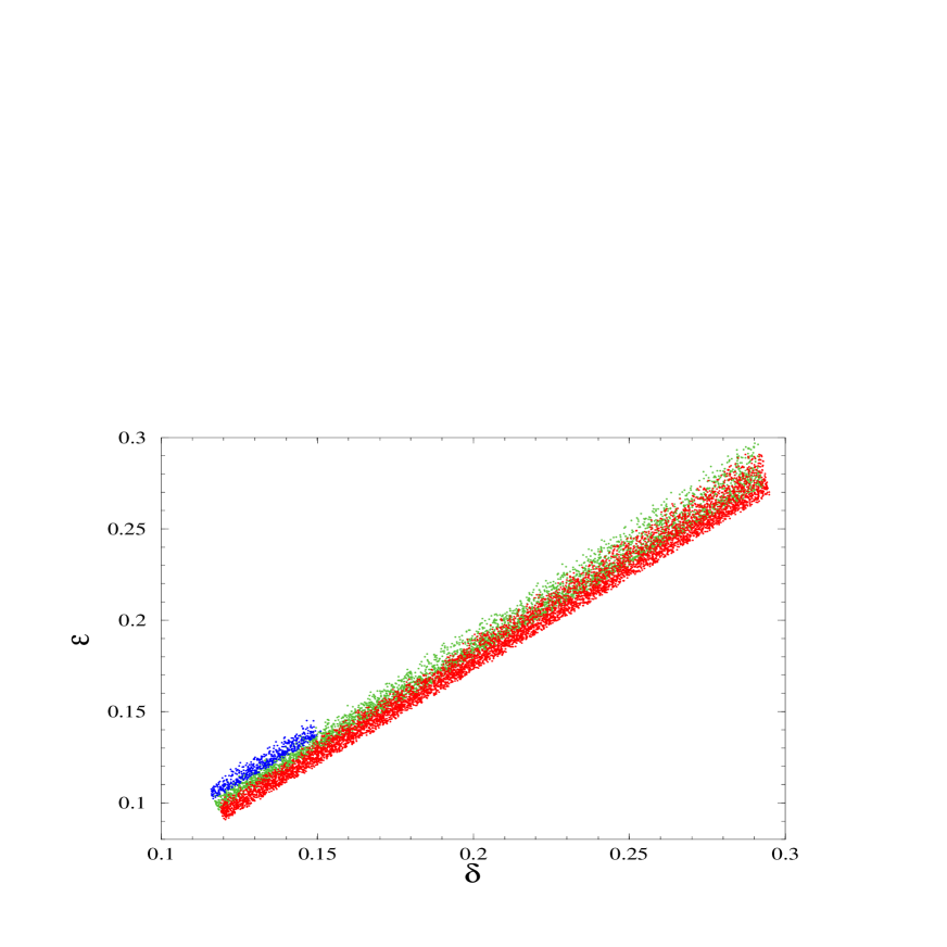
Figure 2: The values of $\epsilon$ and $\delta$ which satisfy the current $3\sigma$ limits from the world neutrino data. The red dots correspond to $m_{0}^{2}=0.0015$ eV², the green dots to $m_{0}^{2}=0.002$ eV² and the blue dots to $m_{0}^{2}=0.003$ eV². The parameter $\theta$ of the mass matrix is allowed to take any possible value.

We show in Fig. 2 the values of the parameters $\epsilon$ and $\delta$ for which our mass matrix predicts values for the oscillation parameters consistent within their current $3\sigma$ allowed limits (given in Eq. (1)-(5)). The parameter $\theta$ of the mass matrix is allowed to vary freely and we show the results for three different values of $m_{0}$ given in the caption of Fig. 2. The allowed values for $\delta$ and $\epsilon$ roughly are seen to correspond to those given by Eqs. (23) and (24). In Table 1 we give the values of the oscillation parameters predicted by our mass matrix for a fixed set of $m_{0}$, $\theta$, $\epsilon$ and $\delta$.

If we denote the deviation of $\theta_{12}$ from its maximal value by $D_{12}=0.5-\sin^{2}\theta_{12}$ and deviation of $\theta_{23}$ from maximality by $D_{23}=0.5-\sin^{2}\theta_{23}$, then

$$D_{12}=\frac{1}{4}\left(3\delta+\epsilon\sqrt{1-4D_{23}^{2}}\right)~{},$$ (25)

while the deviation of $U_{e3}$ from the value of zero is given by

$$U_{e3}=2\sqrt{2}\epsilon D_{23}~{}.$$ (26)

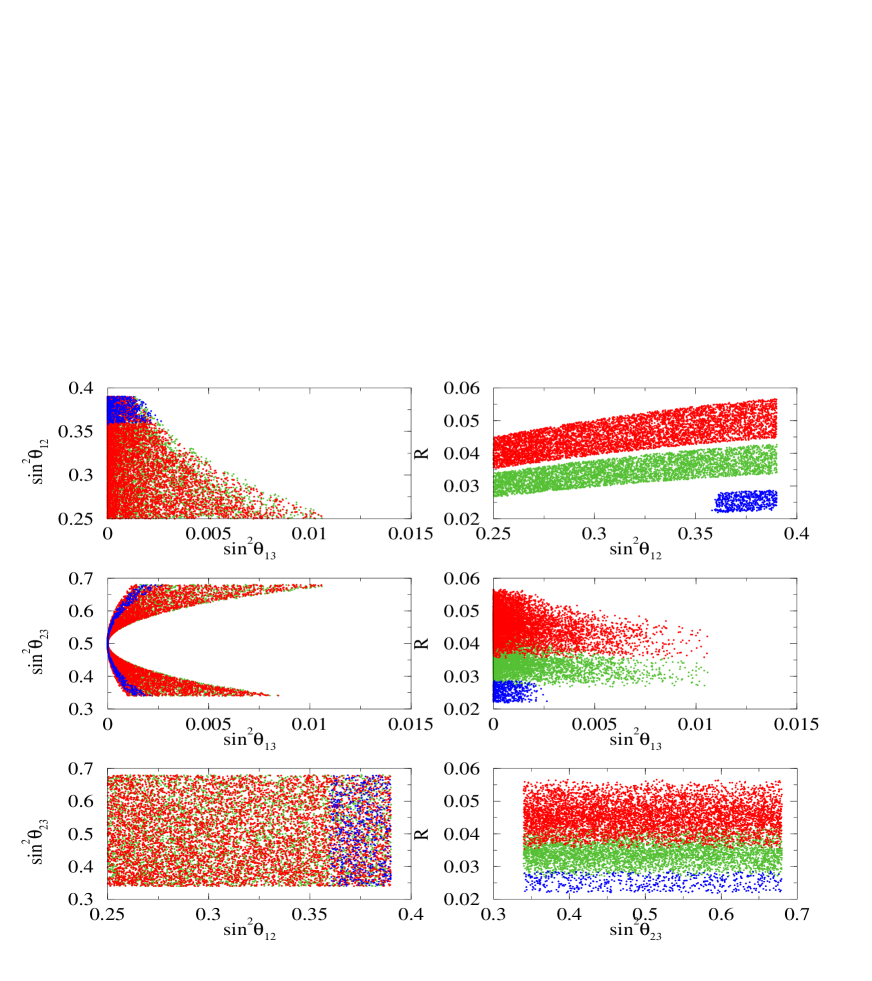
Figure 3: Scatter plot showing the correlation between the values of the oscillation parameters allowed by our perturbed Zee mass matrix. The red dots correspond to $m_{0}^{2}=0.0015$ eV², the green dots to $m_{0}^{2}=0.002$ eV² and the blue dots to $m_{0}^{2}=0.003$ eV².

We show in Fig. 3 the ranges of oscillation parameters predicted by our neutrino mass matrix. In this figure we fix $m_{0}^{2}$ at 0.0015 eV² (red dots), 0.002 eV² (green dots) and 0.003 eV² (blue dots) and let $\epsilon$, $\delta$ and $\theta$ take on any possible value such that the world neutrino data is satisfied at the $3\sigma$ C.L. The left panels show the correlation between the predicted mixing angles while the right panels give the variation of the ratio $R$ with the mixing angles. Note that while the predicted mixing angles and $R$ themselves are independent of $m_{0}^{2}$, the apparent dependence seen in the figure comes from the fact that the mass matrix has to simultaneously explain the individual mass squared differences $\Delta m^{2}_{21}$ and $\Delta m^{2}_{31}$, which depend on $m_{0}^{2}$.

We next turn our attention to the predicted value for the effective mass $|\langle m\rangle|$ that can be observed in neutrino-less double beta decay ($0\nu\beta\beta$) experiments. Since this is given by just the modulus of the $ee$ element of the mass matrix, the predicted effective mass in $0\nu\beta\beta$ is

$$|\langle m\rangle|=2m_{0}\delta.$$ (27)

The prediction for square of the mass observed in tritium beta decay experiments is

$$m_{\beta}^{2}\simeq\frac{m_{0}^{2}}{2}\left[2+\epsilon\sin 2\theta\right],$$ (28)

while the sum of the masses which is constrained from cosmology is predicted in our model to be

$$\sum_{i}|m_{i}|\simeq 2m_{0}\left[1+\frac{1}{2}(\delta-\epsilon\sin 2\theta)\right].$$ (29)

The three observables which depend on the absolute value of the neutrino masses are related in our model as

$$\sum_{i}|m_{i}|\simeq\frac{|\langle m\rangle|}{2}-\frac{2m_{\beta}^{2}}{m_{0}}+4m_{0}.$$ (30)

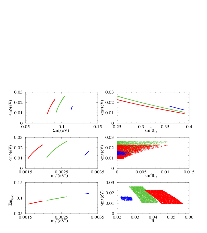
Figure 4: Left columns give the scatter plots showing the correlation between the values of $<m>$, $\sum m_{i}$ and $m_{\beta}$ allowed by our perturbed Zee mass matrix. Right columns show the correlations between $<m>$ and the mixing angles and ratio $R$. The red dots correspond to $m_{0}^{2}=0.0015$ eV², the green dots to $m_{0}^{2}=0.002$ eV² and the blue dots to $m_{0}^{2}=0.003$ eV².

Note that while $|\langle m\rangle|$ depends on $\delta$, $m_{\beta}^{2}$ on $\epsilon$ and $\theta$ and $\sum_{i}|m_{i}|$ on $\epsilon$, $\delta$ and $\theta$, their combination Eq. (30) depends only on $m_{0}$. We show in Fig. 4 the predicted values for the observables in tritium beta decay ($m_{\beta}$), $0\nu\beta\beta$ ($|\langle m\rangle|$) and cosmology ($\sum_{i}|m_{i}|$) in the left panels. The right panels show the correlation between the effective mass $|\langle m\rangle|$ and the oscillation parameters.

We reiterate that our mass matrix has four input parameters namely $m_{0}$, $\delta$, $\epsilon$ and $\theta$. The overall mass scale as well as the mass squared differences are controlled by $m_{0}$, whereas it does not influence the mixing angles at all. Thus $m_{0}$, which is constrained by the solar and atmospheric mass squared differences will have an upper bound coming from experiments on beta decay, neutrinoless double beta decay and cosmology. The mixing angles are controlled by the three other parameters, namely, $\delta$, $\epsilon$ and $\theta$. If we impose the condition of maximal $\theta_{23}$ on the mass matrix, then we must have $\theta=\pi/4$ (cf. Eq. (18)). If we had a $S_{2}$ exchange symmetry between the second and the third generation ($\nu_{\mu}\leftrightarrow\nu_{\tau}$), we will get $\theta=\pi/4$. However, this symmetry also makes $\epsilon=\delta$ and we get the mass matrix given by Eq. (14). The predicted values of the oscillation parameters for this case is given by the first row of Table 1. As discussed before, in this case the mixing angle $\theta_{23}$ is exactly maximal, while $U_{e3}$ is exactly zero. However, note that the solar mass squared difference $\Delta m^{2}_{21}$ is also exactly zero. That the predicted $\theta_{23}$ is maximal, $U_{e3}=0$ and $\Delta m^{2}_{21}=0$ in this case, can also be seen from Eqs. (18), (19) and (15) respectively. This mass matrix is therefore phenomenologically untenable. In order to be able to explain the neutrino oscillation data, this exchange symmetry will have to be broken. This case, as discussed in detail above, is consistent with all observations. The braking of the symmetry forces $\delta\neq\epsilon$ giving a small $\Delta m^{2}_{21}$ and $\theta\neq\pi/4$ causing $\theta_{23}$ to deviate from maximality and $U_{e3}$ from zero – all of which are naturally small, being protected by the approximate $S_{2}$ symmetry.

	Texture parameters				$\sin^{2}2\theta_{\odot}$	$\sin^{2}2\theta_{atm}$	$\Delta m^{2}_{\odot}$	$\Delta m^{2}_{atm}$	$U_{e3}$
	$m_{0}$	$\epsilon$	$\delta$	$\theta$			(eV2)	(eV2)
1	0.039	0.21	0.21	$\pi/4$	0.85	1.0	0	$1.8\times 10^{-3}$	0
2	0.039	0.21	0.236	0.84	0.82	0.99	$9.0\times 10^{-5}$	$1.8\times 10^{-3}$	$0.019$
3	0.039	0.21	0.236	0.73	0.82	0.99	$9.0\times 10^{-5}$	$1.8\times 10^{-3}$	$0.019$

Table 1: Some specific values of input parameters and outputs. In figures more details can be found. It can be noted that atmospheric mixing angle deviates from strict maximality when a non-zero $U_{e3}$ is returned.

3 Discussions on possible models

Let us write Eq. (12) as

$${\cal M}_{ij}=X_{ij}+Y_{ij}$$ (31)

Here $X_{ij}$ is the symmetric off-diagonal part and $Y_{ij}$ is purely diagonal and trace-less. In this paper we work with $SU(3)_{F}$ symmetry as was used in [26] but we consider a further step. We introduce $SU(3)_{F}$ symmetry breaking also; which is obtained by the VEV of an octet Higgs $H_{8}$

$$SU(3)_{F}{<H_{8}>\atop\longrightarrow}SU(2)_{F}\times U(1)_{F}$$ (32)

Leptons are triplets and antileptons are antitriplets whereas quarks are singlets. When $SU(3)_{F}$ symmetry is broken, electron generation becomes a singlet whereas second and third generation remains as a doublet of $SU(2)_{F}$. This helps maximal mixing of atmospheric neutrinos.

$$\pmatrix{L_{e}\cr L_{\mu}\cr L_{\tau}}\rightarrow L_{e}+\pmatrix{L_{\mu}\cr L_{\tau}}$$ (33)

$$\pmatrix{e^{c}\cr\mu^{c}\cr\tau^{c}}\rightarrow e^{c}+\pmatrix{\mu^{c}\cr\tau^{c}}$$ (34)

It is easy to see that this symmetry breaking pattern will be obtained if $H_{8}$ gets a VEV of the form

$$<H_{8}>=\pmatrix{-2&0&0\cr 0&1&0\cr 0&0&1}v$$ (35)

For explaining this let us write down how $SU(3)_{F}$ representations transform under $SU(2)_{F}\times U(1)_{F}$.

$$3 \longrightarrow (1,-2)+(2,1)$$ (36)

$$\overline{3} \longrightarrow (1,2)+(2,-1)$$ (37)

$$8 \longrightarrow (2,3)+(2,-3)+(1,0)+(3,0)$$ (38)

Neither $3$ nor $\overline{3}$ can get VEVs because then we will also break the residual symmetry $SU(2)_{F}\times U(1)_{F}$. The $(1,0)$ component of $8$ must get the VEV; because that will leave the residual $SU(2)_{F}\times U(1)_{F}$ intact. In matrix form the (1,0) component of the octet $H_{8}$ is written in Eq. 35. The $2\times 2$ submatrix in the lower right hand corner is a unit matrix so this $2\times 2$ submatrix is a $SU(2)$ singlet. The trace is vanishing so $U(1)_{F}$ quantum number is zero. Thus this specific symmetry breaking pattern fixes the form of VEV given in Eq. 35.

From the form of the VEV we can see that a residual $SU(2)_{F}$ symmetry remains among the second and the third generation which assures maximality of mixing. The list of leptons Higgs scalars and their $SU(3)_{F}\times SU(3)_{c}\times SU(2)_{L}\times U(1)_{Y}$ representations are

$$FERMIONS$$

$$L=(3,1,2,-1/2)$$ (39)

$$l^{c}=(\overline{3},1,1,1)$$ (40)

$$ZEE~{}~{}MODEL~{}~{}SCALARS$$

$$\phi_{0}=(1,1,2,-1/2)$$ (41)

$$\phi_{1}=(3,1,2,-1/2)$$ (42)

$$\chi=(3,1,1,1)$$ (43)

$$\eta=(1,1,2,-1/2)$$ (44)

$$EXTRA~{}~{}SCALARS$$

$$\Delta_{L}=(3,1,3,1)$$ (45)

$$H_{8}=(8,1,1,0)$$ (46)

First let us explain $Y_{ij}$ term of Eq. (31). The Higgs field $\Delta_{L}$ is a $SU(2)_{L}\times U(1)_{Y}$ triplet as well as a flavor triplet which couples to $\nu_{i}$ and $\nu_{j}$ and gives a direct left handed Majorana mass term of the form $f_{ij}\nu_{i}\nu_{j}v_{L}$, where $v_{L}$ is very small. This mass term acts as the diagonal and trace-less perturbation if the Yukawa coupling $f_{ij}$ is diagonal and trace-less.

Let us explain why the coupling $f_{ij}$ is of this specific form which is diagonal and trace-less. The reason is that it has its origin in a higher dimensional operator of the $SU(3)$ flavor group,

$${f\over M}(3\times 3\times 3\times 8) = {f\over M}~{}L~{}L~{}\Delta_{L}~{}<H_{8}>$$ (48)

At this stage the coupling $f$ does not have any generation index. Putting the value of $<H_{8}>$ from Eqn (35) we get the generation indices as,

$$f_{ij}L_{i}L_{j}\Delta_{L}$$ (49)

Now $f_{ij}$ retains the symmetry between the second and third generation as well as it is diagonal and trace-less.

In the $X_{ij}$ term of Eq. (31) is symmetric with diagonal entries vanishing. It can be generated by the following diagram in Fig 1 in a Zee type model in the presence of our $SU(3)_{F}$ flavor symmetry. The VEV of $\phi_{1}(\overline{3})$ is of the order of electroweak scale. This diagram has been studied very well in the literature. The off diagonal mass matrix is of the form

$$m_{ij}\propto g_{ij}~{}(m^{2}_{j}-m^{2}_{i})$$ (50)

Here $g_{ij}$ is an off-diagonal Yukawa coupling [16, 17]. Actually $g_{ij}$ controls the coupling strength between two lepton doublets and the charged Higgs $\chi^{+}$ in Fig 1. Therefore $SU(2)_{L}$ antisymmetry forces it to be off-diagonal. So, when we multiply $g_{ij}$ by $(m^{2}_{j}-m^{2}_{i})$ the product becomes symmetric with vanishing diagonal elements.

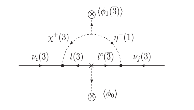
Figure 1: Extra $SU(2)_{L}$ doublet $\phi_{1}$ transform as $\overline{3}$ of $SU(3)$ flavor. It does not couple to fermions at tree level. Quarks do not feel SU(3) flavor in this model. Leptons and antileptons are triplets and antitriplets of SU(3) flavor. $\chi$ is a $SU(2)_{L}$ singlet whereas $\eta$ is a doublet as in minimal Zee model. In bracket we have displayed the $SU(3)$ flavor quantum numbers.

Many different models, in principle, can be constructed which are aesthetically more appealing than this, which will lead to Eq. (12). We do not know which one is right and which is wrong. Typically the first part may be generated by a modified Zee type mechanism and the second part may be generated by a Higgs mechanism or a see-saw mechanism or vice-versa. In this paper we do not focus on the details of the model building apart from citing an example. More models and details based on various flavor groups, will be presented in a future paper [27]. Here we have added the diagonal and trace-less perturbation on a purely phenomenological basis.

4 Conclusions

In this paper we have tried to generate simultaneously a non-zero $U_{e3}$ and LMA solar neutrino mixing angle in a Zee type model by putting in a diagonal and trace-less perturbation. While doing so we have succeeded to keep $\Delta m^{2}_{21}$ and $\Delta m^{2}_{31}$ as well as the atmospheric mixing angle within experimentally allowed ranges. The resulting mass matrix texture is symmetric and trace-less. It has four input parameters and six outputs therefore giving two predictions. When atmospheric neutrino mixing angle is strictly maximal, $U_{e3}$ vanishes. However when atmospheric neutrino mixing angle deviates from strict maximality, a non-vanishing $U_{e3}$ emerges. We studied the correlations between the different oscillation parameters as well as observables depending on the absolute neutrino mass scale, such as the effective mass in neutrino-less double beta decay, mass parameter relevant in beta decay and the sum of the neutrino masses relevant for cosmology. The neutrino mass hierarchy is predicted to be inverted and the oscillation parameters given by this mass matrix are well within the reach of future experiments.

5 Acknowledgements

Work of B.B was financially supported by UGC, New Delhi, under the grant number F.PSU-075/05-06.

References

- [1] B. T. Cleveland et al., Astrophys. J. 496, 505 (1998); V. Gavrin, Talk at Neutrino 2006, Santa Fe, USA, June 14-20, 2006; S. Fukuda et al. [Super-Kamiokande Collaboration], Phys. Lett. B 539, 179 (2002); B. Aharmim et al. [SNO Collaboration], Phys. Rev. C 72, 055502 (2005).
- [2] T. Araki et al. [KamLAND Collaboration], Phys. Rev. Lett. 94, 081801 (2005).
- [3] Y. Ashie et al. [Super-Kamiokande Collaboration], Phys. Rev. D 71, 112005 (2005).
- [4] E. Aliu et al. [K2K Collaboration], Phys. Rev. Lett. 94, 081802 (2005).
- [5] M. Maltoni et al., New J. Phys. 6, 122 (2004), hep-ph/0405172; S. Choubey, arXiv:hep-ph/0509217; A. Bandyopadhyay et al., Phys. Lett. B 608, 115 (2005); G. L. Fogli et al., Prog. Part. Nucl. Phys. 57, 742 (2006).
- [6] P. Huber et al., Phys. Rev. D 70, 073014 (2004).
- [7] A. Bandyopadhyay, S. Choubey and S. Goswami, Phys. Rev. D 67, 113011 (2003); A. Bandyopadhyay et al., Phys. Rev. D 72, 033013 (2005).
- [8] S. Choubey and S. T. Petcov, Phys. Lett. B 594, 333 (2004).
- [9] K. Anderson et al., arXiv:hep-ex/0402041.
- [10] S. Choubey and P. Roy, Phys. Rev. D 73, 013006 (2006); M. C. Gonzalez-Garcia, M. Maltoni and A. Y. Smirnov, Phys. Rev. D 70, 093005 (2004).
- [11] S. T. Petcov and T. Schwetz, Nucl. Phys. B 740, 1 (2006); R. Gandhi et al., Phys. Rev. D 73, 053001 (2006).
- [12] For recent analyzes see: S. Pascoli, S. T. Petcov and T. Schwetz, Nucl. Phys. B 734, 24 (2006); S. Choubey and W. Rodejohann, Phys. Rev. D 72, 033016 (2005).
- [13] S. Schonert, talk at Neutrino 2006, Santa Fe, USA, June 14-20, 2006.
- [14] Peter Doe, talk at Neutrino 2006, Santa Fe, USA, June 14-20, 2006.
- [15] S. Dodelson, talk at Neutrino 2006, Santa Fe, USA, June 14-20, 2006.
- [16] A. Zee, Phys. Lett. B 93, 389 (1980) [Erratum-ibid. B 95, 461 (1980)].
- [17] L. Wolfenstein, Nucl. Phys. B 175, 93 (1980).
- [18] X. G. He, Eur. Phys. J. C 34, 371 (2004).
- [19] P. H. Frampton and S. L. Glashow, Phys. Lett. B 461, 95 (1999); P. H. Frampton, M. C. Oh and T. Yoshikawa, Phys. Rev. D 65, 073014 (2002).
- [20] B. Brahmachari and S. Choubey, Phys. Lett. B 531, 99 (2002).
- [21] T. Kitabayashi, M. Yasue, Int. J. Mod. Phys. A17 2519 (2002); K. Hasegawa, C.S. Lim, K. Ogure, Phys. Rev. D68 053006 (2003); K. R. S. Balaji, W. Grimus and T. Schwetz, Phys. Lett. B 508, 301 (2001).
- [22] D. Black, A. H. Fariborz, S. Nasri and J. Schechter, Phys. Rev. D 62, 073015 (2000); X. G. He and A. Zee, Phys. Rev. D 68, 037302 (2003); W. Rodejohann, Phys. Lett. B 579, 127 (2004); S. S. Masood, S. Nasri and J. Schechter, Phys. Rev. D 71, 093005 (2005).
- [23] C. Jarlskog, M. Matsuda, S. Skadhauge, M. Tanimoto, Phys. Lett. B449, 240 (1999).
- [24] S. T. Petcov, Phys. Lett. B 110, 245 (1982); for more recent studies see, e.g., R. Barbieri et al., JHEP 9812, 017 (1998); A. S. Joshipura and S. D. Rindani, Eur. Phys. J. C 14, 85 (2000); R. N. Mohapatra, A. Perez-Lorenzana and C. A. de Sousa Pires, Phys. Lett. B 474, 355 (2000); Q. Shafi and Z. Tavartkiladze, Phys. Lett. B 482, 145 (2000). L. Lavoura, Phys. Rev. D 62, 093011 (2000); W. Grimus and L. Lavoura, Phys. Rev. D 62, 093012 (2000); T. Kitabayashi and M. Yasue, Phys. Rev. D 63, 095002 (2001); A. Aranda, C. D. Carone and P. Meade, Phys. Rev. D 65, 013011 (2002); K. S. Babu and R. N. Mohapatra, Phys. Lett. B 532, 77 (2002); H. J. He, D. A. Dicus and J. N. Ng, Phys. Lett. B 536, 83 (2002) H. S. Goh, R. N. Mohapatra and S. P. Ng, Phys. Lett. B 542, 116 (2002); G. K. Leontaris, J. Rizos and A. Psallidas, Phys. Lett. B 597, 182 (2004).
- [25] T. Fukuyama and H. Nishiura, hep-ph/9702253; R. N. Mohapatra and S. Nussinov, Phys. Rev. D 60, 013002 (1999); E. Ma and M. Raidal, Phys. Rev. Lett. 87, 011802 (2001); C. S. Lam, Phys. Lett. B 507, 214 (2001); P.F. Harrison and W. G. Scott, Phys. Lett. B 547, 219 (2002); T. Kitabayashi and M. Yasue, Phys. Rev. D 67, 015006 (2003); W. Grimus and L. Lavoura, Phys. Lett. B 572, 189 (2003); J. Phys. G 30, 73 (2004); Y. Koide, Phys. Rev. D 69, 093001 (2004); A. Ghosal, hep-ph/0304090; W. Grimus, A. S. Joshipura, S. Kaneko, L .Lavoura, H. Sawanaka, M. Tanimoto, Nucl. Phys. B 713, 151 (2005); R. N. Mohapatra, SLAC Summer Inst. lecture; http://www-conf.slac.stanford.edu/ssi/2004; JHEP 0410, 027 (2004); A. de Gouvea, Phys. Rev. D 69, 093007 (2004); S. Choubey and W. Rodejohann, Eur. Phys. J. C 40, 259 (2005); R. N. Mohapatra and W. Rodejohann, Phys. Rev. D 72, 053001 (2005); R. N. Mohapatra and S. Nasri, Phys. Rev. D 71, 033001 (2005); R. N. Mohapatra, S. Nasri and H. B. Yu, Phys. Lett. B 615, 231 (2005); Phys. Rev. D 72, 033007 (2005); Y. H. Ahnet al., Phys. Rev. D 73, 093005 (2006); T. Ota and W. Rodejohann, Phys. Lett. B 639, 322 (2006); K. Fuki, M. Yasue, hep-ph/0608042.
- [26] Riazuddin, e-Print Archive: hep-ph/0509124
- [27] B. Brahmachari and S. Choubey, in preparation.
- [28] R. Slansky, Phys. Rept. 79 128 (1981).