ANALYTICAL DESCRIPTION OF HADRON-HADRON SCATTERING VIA PRINCIPLE OF MINIMUM DISTANCE IN SPACE OF STATES
Abstract
In this paper an analytical description of the hadron-hadron scattering is presented by using PMD-SQS-optimum principle in which the differential cross sections in the forward and backward c.m. angles are considered fixed from the experimental data. Experimental tests of the PMD-SQS-optimal predictions, obained by using the available phase shifts, as well as from direct experimental data, are presented. It is shown that the actual experimental data for the differential cross sections of all principal hadron-hadron [nucleon-nucleon, antiproton-proton, mezon-nucleon] scatterings at all energies higher than 2 GeV, can be well systematized by PMD-SQS predictions.
Introduction
The mathematician Leonhard Euler (1707-1783) appears to have been a philosophical optimist having written:
”For since the fabric of the universe is most perfect and the work of a most wise Creator, nothing at all takes place in the universe in which some rule of maximum or minimum does not appear. Wherefore, there is absolutely no doubt that every effect in universe can be explained as satisfactory from final causes themselves the aid of the method of Maxima and Minima, as can from the effective causes”.
Yet this brilliant idea produced many strikingly simple formulations of certain complex laws of nature. From historical point of view the earliest optimum principle was proposed by Heron of Alexandria (125 B.C.) in connection with the behavior of light. Thus, Heron proved mathematically the following first genuine scientific minimum principle of physics: that light travels between two points by shortest path. In fact the Archimedean definition of a straight line as the shortest path between two points was an early expression of a variational principle, leading to the modern idea of a geodesic path. In fact in the same spirit, Hero of Alexandria explained the paths of reflected rays of light based on the principle of minimum distance (PMD), which Fermat (1657) reinterpreted as a principle of least time, Subsequently, Maupertuis and others developed this approach into a general principle of least action, applicable to mechanical as well as to optical phenomena. Of course, a more correct statement of these optimum principles is that systems evolve along stationary paths, which may be maximal, minimal, or neither (at an inflection point). Laws of mechanics were first formulated in terms of minimum principles. Optics and mechanics were brought together by a single minimum principle conceived by W. R. Hamilton. From Hamilton’s single minimum principle could be obtained all the optical and mechanical laws then known. But the effort to find optimum principles has not been confined entirely to the exact sciences. In modern time the principles of optimum are extended to all sciences. So, there exists many minimum principle in action in all sciences, such as: principle of minimum action, principle of minimum free-energy, minimum charge, minimum entropy production, minimum Fischer information, minimum potential energy, minimum rate of energy dissipation, minimum dissipation, minimum of Chemical distance, minimum cross entropy, minimum complexity in evolution, minimum frustration, minimum sensitivity, etc. So, a variety of generalizations of classical variational principles have appeared, and we shall not describe them here.
Next, having in mind this kind of optimism in the paper [1-16] we introduced and investigated the possibility to construct a predictive analytic theory of the elementary particle interaction based on the principle of minimum distance in the space of quantum states (PMD-SQS). So, choosing the partial transition amplitudes as the system variational variables and the “distance” in the Hilbert space of the quantum transitions as a measure of the system effectiveness expressed in function of partial transition amplitudes we obtained the results [1-16]. These results proved that the principle of minimum distance in space of quantum states (PMD-SQS) can be chosen as variational principle by which we can find the analytic expressions of the partial transition amplitudes In this project by using the S-matrix theory the minimum principle PMD-SQS will be formulated in a general mathematical form. We prove that the new analytic theory of the quantum physics based on PMD-SQS is completely described with the aid of the reproducing kernels from RKHS of the transition amplitudes. [1-5].
Therefore, in Ref. [1] by using reproducing kernel Hilbert space (RKHS) methods [3-5,17], we described the quantum scattering of the spinless particles by a principle of minimum distance in the space of quantum states (PMD-SQS). Some preliminary experimental tests of the PMD-SQS, even in the crude form [1] when the complications due to the particle spins are neglected, showed that the actual experimental data for the differential cross sections of all principal hadron-hadron [nucleon-nucleon, antiproton-proton, mezon-nucleon] scatterings at all energies higher than 2 GeV, can be well systematized by PMD-SQS predictions (see the papers [1,], Moreover, connections between the PMD-SQS and the maximum entropy principle for the statistics of the scattering quantum channels was also recently established by introducing quantum scattering entropies: Sθand SJ[5-7]. Then, it was shown that the experimental pion-nucleon as well as pion-nucleus scattering entropies are well described by optimal entropies and that the experimental data are consistent with the principle of minimum distance in the space of quantum states (PMD-SQS) }[1]. However, the PMD-SQS in the crude form [1] cannot describe the polarization J-spin effects.
In this paper an analytical description of the hadron-hadron scattering is presented by using PMD-SQS-optimum principle in which the differential cross sections in the forward (x=+1) and backward (x=-1) directions are considered fixed from the experimental data. An experimental test of the optimal prediction on the logarithmic slope b is performed for the pion-nucleon and kaon-nucleon scatterings at the forward c.m. angles.
2. Description of pion-nucleon scattering via principle of minimum distance in space of quantum states (PMD-SQS)
First we present the basic definitions on the hadronic scattering:
| (1) |
Therefore, let and , be the scattering helicity amplitudes of the mezon-nucleon scattering process (see ref.[14]) written in terms of the partial helicities sand as follows
| (2) |
where the rotation functions are defined as
| (3) |
where are Legendre polinomials, , x being the c.m. scattering angle. The normalisation of the helicity amplitudes and , is chosen such that the c.m. differential cross section is given by
| (4) |
Then, the elastic integrated cross section is given by
| (5) |
Now, let us consider the following optimization problem:
| (6) |
when and are fixed.
We proved that the solution of this optimization problem is given by the following results :
| (7) |
| (8) |
where the functions K(x,y) are the reproducing kernels [3-5] expressed in terms of rotation function by
| (9) |
| (10) |
while the optimal angular momentum is given by
| (11) |
Now, let us consider the logarithmic slope b of the forward diffraction peak defined by
| (12) |
Then, using the definition of the rotation functions, from (7)-(11) we obtain the optimal slope
| (13) |
Finally, we note that in ref. [13] we proved the following optimal inequality
| (14) |
which includes in a more general and exact form the unitarity bounds derived by Martin [18] and Martin-Mac Dowell [19] (see also ref.[20]) and Ion [1,21]. Indeed, since , and
| (15) |
(Wik inequality) from the bound (14), we get
| (16) |
| (17) |
| (18) |
| (19) |
3. Experimental tests of the PMD-SQS-optimal predictions
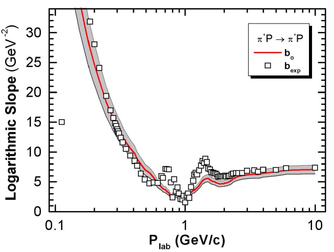
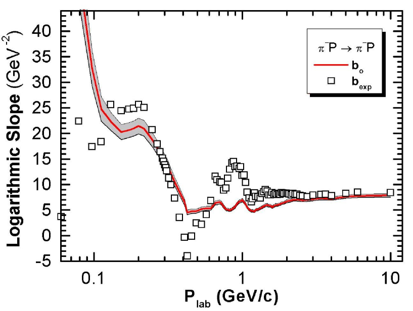
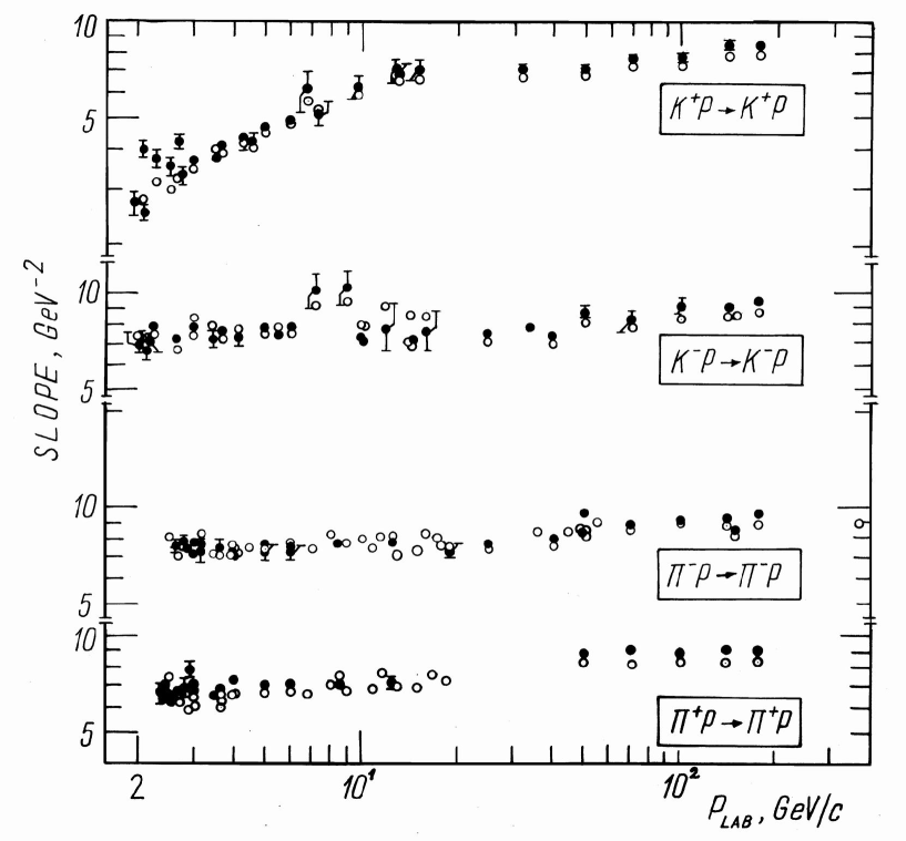
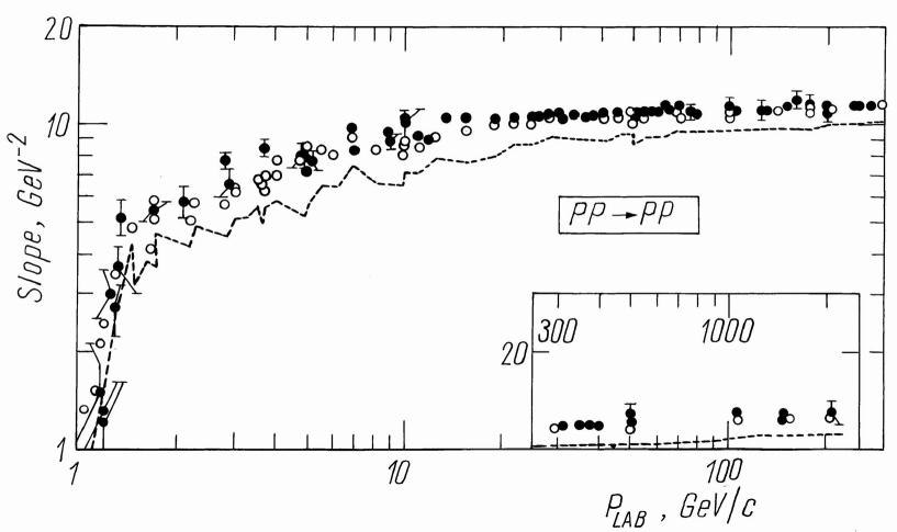
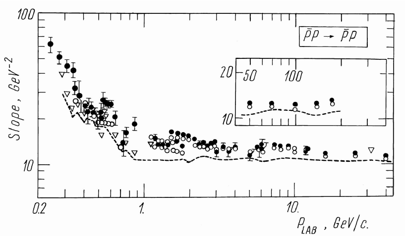
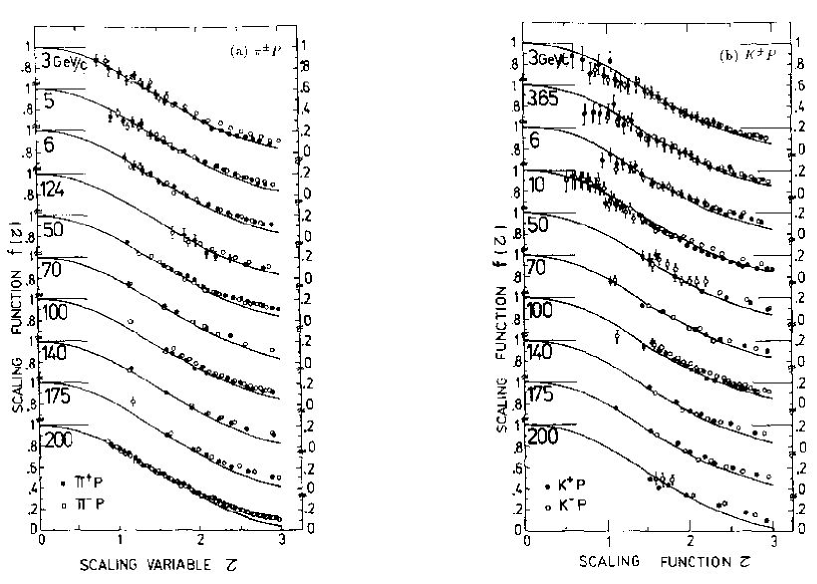
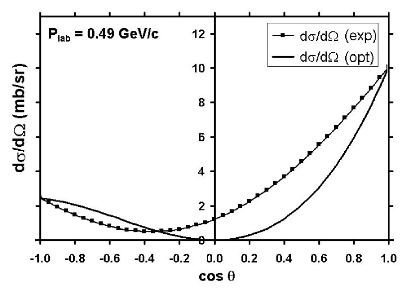
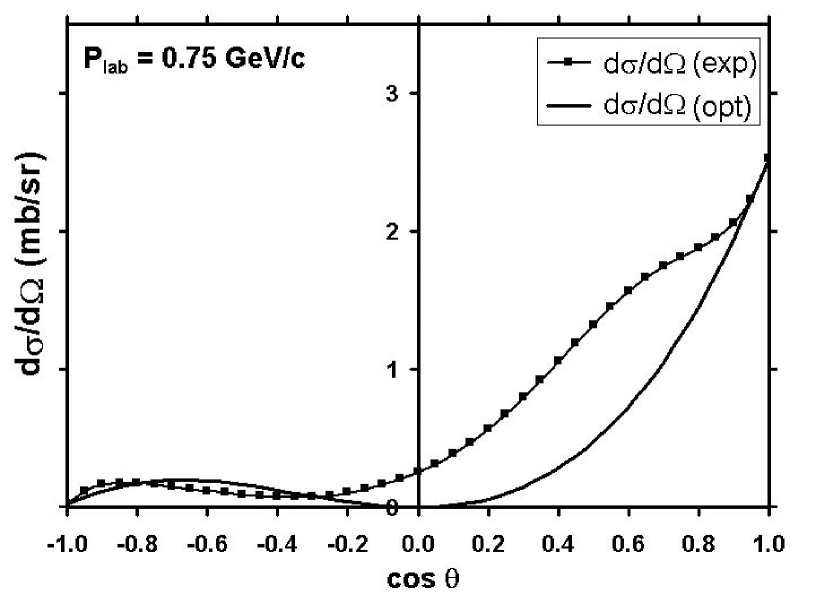
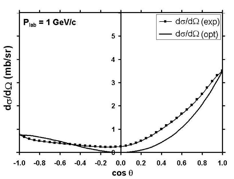
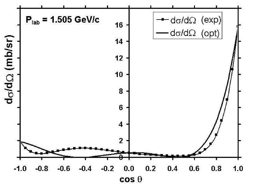
For an experimental test of the optimal result (14) the numerical values of the slopes and are calculated directly by reconstruction of the helicity amplitudes from the experimental phase shifts (EPS) solutions of Holer et al. [23] and also directly from the experimental data. The results are displayied in Fig 1-5. Moreover, we calculated from the experimental data (see [24-29]) the following physical quantities:
SCALING FUNCTION:
| (20) |
SCALING VARIABLE:
| (21) |
and compared with the values of the PMD-SQS-optimal predictions obtained from
OPTIMAL SCALING FUNCTION:
| (22) |
The results are presented in Fig. 6. We must note that the approximation in (22) is derived by using the relation
| (23) |
Where are Bessel functions of order .
4. Conclusions
The main results and conclusions obtained in this paper can be summarized as follows:
In this paper an analytical description of the hadron-hadron scattering is presented by using PMD-SQS-optimum principle in which the differential cross sections in the forward (x=+1) and backward (x=-1) directions are considered fixed from the experimental data. So, choosing the partial transition amplitudes as the system variational variables and the “distance” in the Hilbert space of the quantum transitions as a measure of the system effectiveness expressed in function of partial transition amplitudes we obtained the results [1-16].
(i) The PMD-SQS optimal dominance in hadron-hadron scattering at small transfer momenta for GeV/c is a fact well evidenced experimentally by the results presented in Figs. 1-6. This conclusion can be also extended in low energy region.
(ii) In the low energy region, the optimal slope (13) is in good agreement with the experimental data in some domains of energy between the resonances positions or/and in the region corresponding to the diffractive resonances see Figs. 1-2 and Figs. 7-10.
(iii) We find that the presented experimental tests prove that the principle of minimum distance in space of quantum states (PMD-SQS) can be chosen as variational principle by which we can find the analytic expressions of the partial transition amplitudes.
Finally, we hope that our results are encouraging for an analytic description of the quantum scattering in terms of an optimum principle, namely, the principle of minimum distance in space of quantum state (PMD-SQS) introduced by us in ref. [1].
5. References
[1] D.B.Ion ”Description of quantum scattering via principle of minimum distance in space of states”, Phys. Lett. B 376 (1996) 282.
[2] D.B.Ion and M.L.D.Ion,”Isospin quantum distances in hadron-hadron scatterings”, Phys. Lett. B 379 (1996) 225.
[3] D.B.Ion and H. Scutaru, ”Reproducing kernel Hilbert space and optimal state description of hadron-hadron scattering”, Int. J. Theor. Phys. 24 (1985) 355.
[4] D.B.Ion, ”Reproducing kernel Hilbert spaces and extremal problems for scattering of particles with arbitrary spins”, Int. J. Theor. Phys. 24 (1985) 1217.
[5] D.B.Ion ”Scaling and S-channel helicity conservation via optimal state description of hadron-hadron scattering”, Int. J. Theor. Phys. 25 (1986) 1257.
[6] D.B.Ion and M.L.D.Ion, ”Information entropies in pion-nucleon scattering and optimal state analysis”,
Phys. Lett. B 352 (1995) 155.
[7] D.B.Ion and M.L.D.Ion, ”Entropic lower bound for quantum scattering of spineless particles”, Phys. Rev. Lett. 81 (1998) 5714.
[8] M.L.D.Ion and D.B.Ion, ”Entropic uncertainty relations for nonextensive quantum scattering,
Phys. Lett. B 466 (1999) 27-32.
[9] M.L.D.Ion and D.B.Ion, ”Optimal bounds for Tsallis-like entropies in quantum scattering of spinless particles”, Phys. Rev. Lett. 83 (1999) 463.
[10] M.L.D.Ion and D.B.Ion, ”Angle-angular-momentum entropic bounds and optimal entropies for quantum scattering of spineless particles”, Phys. Rev. E 60 (1999) 5261.
[11] D. B. Ion and M. L.D. Ion, ”Limited entropic uncertainty as a new principle in quantum physics”, Phys. Lett. B 474 (2000) 395.
[12] M.L.D.Ion and D.B.Ion, ”Strong evidences for correlated nonextensive statistics in hadronic scatterings”, Phys. Lett. B 482 (2000) 57.
[13] D. B. Ion and M. L.D. Ion, ”Optimality entropy and complexity in quantum scattering”,
Chaos Solitons and Fractals, 13 (2002) 547.
[14] D. B. Ion and M. L.D.Ion, ”Evidences for nonextensive statistics conjugation in hadronic scatterings systems”, Phys. Lett. B 503 (2001) 263.
[15] D. B. Ion and M. L. D.Ion, ”New nonextensive quantum entropy and strong evidences for the equilibrium of quantum hadronic states”, Phys. Lett. B 519 (2001) 63.
[16] D. B. Ion and M.D. Ion, Nonextensive statistics ans saturation of PMD-SQS-optimality limits in hadronic scattering”, Physica A 340 (2004) 501.
[17] N. Aronsjain, Proc. Cambridge Philos. Soc. 39 (1943) 133, Trans. Amer. Math. Soc. 68 (1950) 337; S. Bergman, The Kernel Function and Conformal mapping, Math. Surveys No 5. AMS, Providence, Rhode Island, 1950; S. Bergman,and M. Schiffer Kernel Functions and Eliptic Differential Equations in Mathematical Physics, Academic Press, New York, 1953; A. Meschkowski, Hilbertische Raume mit Kernfunction, Springer Berlin, 1962; H.S. Shapiro, Topics in Approximation Theory, Lectures Notes in Mathematics, No 187, Ch. 6, Springer, Berlin, 1971
[18] A. Martin, Phys. Rev. 129,1432 (1963).
[19] S. W. MacDowell and A. Martin, Phys. Rev. 135 B, 960 (1964).
[20] S. M. Roy, Phys. Rep. 5C, 125 (1972).
[21] D. B. Ion, St. Cerc. Fiz. 43, 5 (1991).
[22] See the books: N. R. Hestenes, Calculus of variations and optimal control theory, John Wiley&Sons, Inc., 1966, and also V. M. Alecseev, V. M. Tihomirov and S. V. Fomin, Optimalinoe Upravlenie, Nauka, Moskow,1979.
[23] Hohler, F. Kaiser, R. Koch, E. Pitarinen, Physics Data, Handbook of Pion Nucleon Scattering, 1979, Nr. 12-1.
[24] D. B. Ion and M. L. Ion, A new optimal bound on logarithmic slope of elastic hadro-hadron scattering, ArXiv: hep-ph/0501146 v1 16 Jan 2005.
[25] For extensive experimental literature see: J. Bystricky –Landolt-Bornstein, New Series, Group I-Vol 9a, Nucleon-Nucleon and Kaon-Nucleon Scattering (1980).
[26] D.B.Ion, C. Petrascu, Rom. Journ. Phys. 37 (1992) 569-575.
[27] D.B.Ion, C. Petrascu and A. Rosca, Rom. Journ. Phys. 37 (1992) 977-989.
[28] D.B.Ion, C. Petrascu, Rom. Journ. Phys. 38 (1993) 23-29.
[29] D.B.Ion, C. Petrascu, A. Rosca and V. Topor, Rom. Journ. Phys. 39 (1994) 213-221.