Observables sensitive to absolute neutrino masses:
A reappraisal after WMAP-3y and first MINOS results

Abstract

In the light of recent neutrino oscillation and non-oscillation data, we revisit the phenomenological constraints applicable to three observables sensitive to absolute neutrino masses: The effective neutrino mass in single beta decay $(m_{\beta})$; the effective Majorana neutrino mass in neutrinoless double beta decay $(m_{\beta\beta})$; and the sum of neutrino masses in cosmology $(\Sigma)$. In particular, we include the constraints coming from the first Main Injector Neutrino Oscillation Search (MINOS) data and from the Wilkinson Microwave Anisotropy Probe (WMAP) three-year (3y) data, as well as other relevant cosmological data and priors. We find that the largest neutrino squared mass difference is determined with a 15% accuracy (at $2\sigma$) after adding MINOS to world data. We also find upper bounds on the sum of neutrino masses $\Sigma$ ranging from $\sim 2$ eV (WMAP-3y data only) to $\sim 0.2$ eV (all cosmological data) at $2\sigma$, in agreement with previous studies. In addition, we discuss the connection of such bounds with those placed on the matter power spectrum normalization parameter $\sigma_{8}$. We show how the partial degeneracy between $\Sigma$ and $\sigma_{8}$ in WMAP-3y data is broken by adding further cosmological data, and how the overall preference of such data for relatively high values of $\sigma_{8}$ pushes the upper bound of $\Sigma$ in the sub-eV range. Finally, for various combination of data sets, we revisit the (in)compatibility between current $\Sigma$ and $m_{\beta\beta}$ constraints (and claims), and derive quantitative predictions for future single and double beta decay experiments.

I Introduction

One of the greatest challenges in current neutrino physics is to establish the absolute masses $(m_{1},m_{2},m_{3})$ of the three neutrino mass eigenstates $(\nu_{1},\nu_{2},\nu_{3})$, for which there is ample experimental evidence of mixing with the three neutrino flavor eigenstates $(\nu_{e},\nu_{\mu},\nu_{\tau})$ through a unitary matrix $U(\theta_{12},\theta_{23},\theta_{13})$, where $\theta_{ij}$ are the mixing angles PDG4 .

Atmospheric, solar, reactor, and accelerator neutrino oscillation experiments constrain two squared mass differences, $\delta m^{2}$ and $\Delta m^{2}$ (with $\delta m^{2}\ll\Delta m^{2}$), parametrized as

$$(m^{2}_{1},\,m^{2}_{2},\,m^{2}_{3})=\frac{m^{2}_{1}+m^{2}_{2}}{2}+\left(-\frac{\delta m^{2}}{2},\,+\frac{\delta m^{2}}{2},\,\pm\Delta m^{2}\right)\ ,$$ (1)

where the cases $+\Delta m^{2}$ and $-\Delta m^{2}$ distinguish the so-called normal hierarchy (NH) and inverted hierarchy (IH), respectively. The same data also measure $\theta_{12}$ and $\theta_{23}$, and place upper bounds on $\theta_{13}$ (see PPNP ; Viss for recent reviews).

Non-oscillation neutrino data from single $\beta$ decay, from neutrinoless double $\beta$ decay ($0\nu 2\beta$), and from cosmology, add independent constraints on the absolute neutrino masses, through their sensitivity to the observables PDG4

$$m_{\beta} = \left[c^{2}_{13}c^{2}_{12}m^{2}_{1}+c^{2}_{13}s^{2}_{12}m^{2}_{2}+s^{2}_{13}m^{2}_{3}\right]^{\frac{1}{2}}\ ,$$ (2)

$$m_{\beta\beta} = \left|c^{2}_{13}c^{2}_{12}m_{1}+c^{2}_{13}s^{2}_{12}m_{2}e^{i\phi_{2}}+s^{2}_{13}m_{3}e^{i\phi_{3}}\right|\ ,$$ (3)

$$\Sigma = m_{1}+m_{2}+m_{3}\ ,$$ (4)

respectively (with $c_{ij}=\cos\theta_{ij}$ and $s_{ij}=\sin\theta_{ij}$, while $\phi_{2,3}$ are unknown Majorana phases).

In a previous work fogli , a global analysis of world oscillation and non-oscillation data was performed, with the purpose of showing the interplay and the (in)compatibility of different data sets in constraining the $(m_{\beta},m_{\beta\beta},\Sigma)$ parameter space. In this work, we revisit such constraints in the light of two recent relevant developments: the first results from the Main Injector Neutrino Oscillation Search (MINOS) MINOS (see Sec. II), and the three-year (3y) results from the Wilkinson Microwave Anisotropy Probe (WMAP) WMAP3 (see sec. IV), which have a direct impact on $\Delta m^{2}$ and $\Sigma$, respectively. In Sec. II we show that, after MINOS, the $\Delta m^{2}$ parameter is globally determined with an accuracy of 15% at $2\sigma$. In Sec. V we discuss the degeneracy between $\Sigma$ and the cosmological parameter $\sigma_{8}$ (which normalizes the matter power spectrum PDG4 ; WMAP3 ), as well as the breaking of such degeneracy with the addition of further cosmological data, which strenghten the $2\sigma$ upper bound on $\Sigma$ from $\sim 2$ eV (WMAP 3y only) to $\sim 0.2$ eV (all cosmological data). Such limits on $\Sigma$ are in agreement with other recent analyses WMAP3 ; Seljak:2006bg ; goobar ; fukugita ; raffelt ; cirelli ; pastor . Older $\beta$ and $0\nu 2\beta$ results, including the $0\nu 2\beta$ signal claim of Kl04 , are also briefly reviewed (see Sec. III). In Sec V we discuss the issues of the (in)compatibility among the previous data sets and of their possible combinations and constraints in the parameter space $(m_{\beta},m_{\beta\beta},\Sigma)$. In particular, we show that the case with “WMAP 3y only” still allows a global combination (at the $2\sigma$ level) with the $0\nu 2\beta$ signal claimed in Kl04 , while the addition of other cosmological data excludes this combination (at the same or higher significance level). Quantitative implications for future $\beta$ and $0\nu 2\beta$ decay searches are worked out for various combinations of current data (Secs. V and VI). Conclusions are given in Sec. VII.

II Oscillation parameters after first MINOS results

The oscillation parameters $(\delta m^{2},\,\theta_{12})$ are essentially determined by the solar and KamLAND reactor neutrino data combination, which we take from PPNP (not altered by slightly updated Gallium data gavrin , as we have checked). The corresponding $2\sigma$ ranges are PPNP :

$$\delta m^{2} = 7.92\,(1\pm 0.09)\times 10^{-5}\mathrm{\ eV}^{2}\ ,$$ (5)

$$\sin^{2}\theta_{12} = 0.314\,(1^{+0.18}_{-0.15})\ .$$ (6)

The parameters ($\Delta m^{2},\sin^{2}\theta_{23}$) are dominated by atmospheric and accelerator $\nu$ data, within the CHOOZ CHOOZ bounds on $\sin^{2}\theta_{13}$ (see PPNP for details). After the review PPNP , oscillation results have been finalized for the Super-Kamiokande (SK) atmospheric $\nu$ experiment SKatm and for the KEK-to-Kamioka (K2K) accelerator $\nu$ experiment K2K . The SK+K2K analysis in PPNP , however, contains most of the final SK and K2K statistics, and is not updated here.

New accelerator data in the $\nu_{\mu}\to\nu_{\mu}$ disappearance channel have recently been released by the MINOS experiment MINOS . The MINOS data significantly help to constrain the $\Delta m^{2}$ parameter MINOS , while they are less sensitive to $\theta_{23}$ (as compared with atmospheric data SKatm ), and are at present basically insensitive to $\sin^{2}\theta_{13}$, although some sensitivity will be gained through future searches in the $\nu_{\mu}\to\nu_{e}$ appearance channel. They are also insensitive to the parameters $(\delta m^{2},\,\theta_{12})$, whose main effect (at $\theta_{13}\simeq 0$) is to change the oscillation phase by a tiny fractional amount $0.5\,\delta m^{2}\cos 2\theta_{12}/\Delta m^{2}\simeq 0.6\times 10^{-2}$ (see, e.g., PPNP ), which is negligible within current uncertainties. Therefore, the usual two-family approximation—also adopted in the official MINOS analysis PPNP —is currently appropriate to study MINOS data.

In the absence of a detailed description of the procedure used by the MINOS collaboration for the data analysis, we provisionally include their constraints on the parameters $(\Delta m^{2},\,\sin^{2}\theta_{23})$ through an empirical parametrization of the $\chi^{2}$ statistical function,

$$\chi^{2}_{\mathrm{MINOS}}=\left(\frac{x-1}{0.134}\right)^{2}+\left(\frac{y\cdot x^{0.76}-2.74}{0.27}\right)^{2}\ ,$$ (7)

where $x=\sin^{2}(2\theta_{23})$ and $y=\Delta m^{2}/(10^{-3}\ \mathrm{eV}^{2})$. This parametrization accurately reproduces the official MINOS bounds in the plane ($\Delta m^{2},\sin^{2}2\theta_{23}$) MINOS (at least in the relevant region at relatively large mixing angles, $\sin^{2}\theta_{23}\in[0.3,0.7]$). A more proper analysis will be performed when further experimental and statistical details will be made public by MINOS.

By adding the above $\chi^{2}$ function in the global analysis of neutrino oscillation data performed in PPNP , we obtain the following $2\sigma$ allowed ranges:

$$\Delta m^{2} = 2.6\,(1^{+0.14}_{-0.15})\times 10^{-3}\mathrm{\ eV}^{2}\ ,$$ (8)

$$\sin^{2}\theta_{23} = 0.45\,(1^{+0.35}_{-0.20})\ ,$$ (9)

which noticeably improve the previous bounds in PPNP . In particular, the $2\sigma$ error on $\Delta m^{2}$ is reduced from $\sim 24\%$ PPNP to $\sim 15\%$ after the inclusion of MINOS data.

The error reduction for $\Delta m^{2}$ also reduces the spread of the (dominant) CHOOZ limits on $\sin^{2}\theta_{13}$ CHOOZ , which are $\Delta m^{2}$-dependent. Therefore, MINOS indirectly provides a slight improvement of the previous bounds on $\sin^{2}\theta_{13}$ PPNP , which are now updated at $2\sigma$ as:

$$\sin^{2}\theta_{13}=(0.8^{+2.3}_{-0.8})\times 10^{-2}\ .$$ (10)

Equations (5), (6), (8), (9) and (10) represent our up-to-date evaluation of the neutrino oscillation parameters (at 95% C.L.).

Figure 1 shows the comparison between the limits obtained on $(\Delta m^{2},\,\sin^{2}\theta_{23},\,\sin^{2}\theta_{13})$ before MINOS (dashed, from PPNP ) and after MINOS (solid, this work), in terms of standard deviations from the best fit (i.e., in terms of $\sqrt{\Delta\chi^{2}}$, where $\Delta\chi^{2}$ is the fitting function to all oscillation data PPNP ). The impact of MINOS on the $\Delta m^{2}$ parameter is rather significant, and the related uncertainties appear now to scale almost linearly and symmetrically. The analogous figure (not shown) for the $(\delta m^{2},\,\sin^{2}\theta_{12})$ parameters—which are not affected by MINOS data—can be found in PPNP .

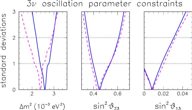
Figure 1: Constraints placed by neutrino oscillation data on the parameters ($\Delta m^{2},\,\sin^{2}\theta_{23},\,\sin^{2}\theta_{13}$), which are affected by the inclusion of the first MINOS results. The results are shown in terms of standard deviations from the best fit. Solid (dashed) lines refers to all neutrino oscillation data with (without) MINOS.

III Input from single and double beta decay searches

Single $\beta$-decay experiments probe the effective electron neutrino mass parameter $m_{\beta}$, at least in first approximation. The most stringent constraints on $m_{\beta}$ are placed by the Mainz and Troitsk experiments Eite , the latter being affected by still unexplained time-dependent systematics. We assume that both the Mainz and Troitsk results can be taken at face value and combined as in PPNP ; fogli , obtaining at $2\sigma$:

$$m_{\beta}<1.8\mathrm{\ eV}\ .$$ (11)

If only the Mainz results were used, this limit would be slightly relaxed ($m_{\beta}<2.2$ eV). In any case, the above bound is relatively weak and has almost no impact in the following analyses, except for one scenario (see Case $1^{+}$ in Sec. V A).

Double beta decay searches with no final-state neutrinos have not reported positive signals so far Elli , except in the most sensitive (⁷⁶Ge) detector to date (Heidelberg-Moscow experiment), where part of the collaboration has claimed a signal at $>4\sigma$ level Kl04 , recently promoted to $>6\sigma$ level by a pulse-shape analysis Kl06 . This claim is still considered as controversial Elli and we shall discuss its implications with due care in the following sections. In any case, any claim or limit on the $0\nu 2\beta$ decay half-life ($T^{0\nu}_{1/2}$) in a candidate nucleus constrains the effective Majorana mass ($m_{\beta\beta}$) through the relation

$$m^{2}_{\beta\beta}=\frac{m^{2}_{e}}{C_{mm}\,T^{0\nu}_{1/2}}\ ,$$ (12)

in the assumption that the $0\nu 2\beta$ process proceeds only through light Majorana neutrinos (and not through new interactions or particles) Elli . The relevant nuclear physics is included in the matrix element $C_{mm}$, which must be theoretically calculated.

Since the above relation is non-linear, and since all the quantities involved (except the electron mass $m_{e}$) are subject to large uncertainties, we prefer to linearize Eq. (12) and to deal with more “tractable” uncertainties by using logarithms as in fogli :

$$2\log_{10}\left(\frac{m_{\beta\beta}}{\mathrm{eV}}\right)=2\log_{10}\left(\frac{m_{e}}{\mathrm{eV}}\right)-\log_{10}\left(\frac{C_{mm}}{\mathrm{yr}^{-1}}\right)-\log_{10}\left(\frac{T^{0\nu}_{1/2}}{\mathrm{yr}}\right)\ .$$ (13)

In the following, it is understood that linear error propagation is applied to the above “logs” (e.g., $\log C_{mm}$) rather than to the exponentiated quantities (e.g., $C_{mm}$).

Table 1: Our summary of the estimated $0\nu 2\beta$ nuclear matrix elements $C_{mm}$ and their $\pm 2\sigma$ errors (in logarithmic scale) for seven relevant nuclei, as derived from Ref. faessler . See the text for details.

Nucleus	$\log_{10}(C_{mm}/\mathrm{yr}^{-1})\pm 2\sigma$
76Ge	$-13.36\pm 0.10$
82Se	$-12.83\pm 0.14$
100Mo	$-13.13\pm 0.20$
116Cd	$-12.96\pm 0.24$
128Te	$-14.32\pm 0.29$
130Te	$-12.98\pm 0.30$
136Xe	$-13.41\pm 0.56$

In our analysis, we take the theoretical input for $\log C_{mm}$ (central values and errors) from the quasi-random phase approximation (QRPA) calculations in Ref. faessler , where it has been shown that the nuclear uncertainties can be significantly constrained (and reduced) by requiring consistency with independent $2\nu 2\beta$ decay data (when available). More precisely, for a given nucleus, we take the logarithms of the minimum and maximum values of $C_{mm}$ from the $\pm 1\sigma$ ranges reported in the last column of Table 1 in faessler ; then, by taking half the sum and half the difference of these extremal values we get, respectively, our default central value and $1\sigma$ error for $\log C_{mm}$ ($2\sigma$ errors are just doubled). Table 1 shows a summary of the $\log C_{mm}$ values and their $2\sigma$ errors derived in this way, and used hereafter.

With the theoretical input for $C_{mm}({}^{76}\mathrm{Ge})$ from Table 1, the $0\nu 2\beta$ claim of Kl04 is transformed in the following $2\sigma$ range for $m_{\beta\beta}$:

$$\log_{10}(m_{\beta\beta}/\mathrm{eV})=-0.23\pm 0.14\ \ (0\nu 2\beta\mathrm{\ claim\ accepted})\ ,$$ (14)

i.e., $0.43<m_{\beta\beta}<0.81$ (at $2\sigma$, in eV). See also fogli for our previous estimated range (with more conservative theoretical uncertainties). As in fogli , we consider the possibility that $T^{0\nu}_{1/2}=\infty$ is allowed (i.e., that the claimed $0\nu 2\beta$ signal is incorrect), in which case the experimental lower bound on $m_{\beta\beta}$ disappears, and only the upper bound at $2\sigma$ remains:

$$\log_{10}(m_{\beta\beta}/\mathrm{eV})=-0.23^{+0.14}_{-\infty}\ (0\nu 2\beta\mathrm{\ claim\ not\ accepted})\ .$$ (15)

IV Input from cosmological data

The neutrino contribution to the overall energy density of the universe can play a relevant role in large scale structure formation and leave key signatures in several cosmological data sets. More specifically, neutrinos suppress the growth of fluctuations on scales below the horizon when they become non relativistic. Massive neutrinos with $\Sigma=m_{1}+m_{2}+m_{3}$ in the (sub)eV range would then produce a significant suppression in the clustering on small cosmological scales (see pastor for a recent review).

The method that we adopt to derive bounds on $\Sigma$ is based on the publicly available Markov Chain Monte Carlo (MCMC) package cosmomc Lewis:2002ah . We sample the following set of cosmological parameters, adopting flat priors on them: the physical baryon, cold dark matter, and massive neutrino densities ($\omega_{b}=\Omega_{b}h^{2}$, $\omega_{c}=\Omega_{c}h^{2}$ and $\Omega_{\nu}h^{2}$, respectively), the ratio of the sound horizon to the angular diameter distance at decoupling ($\theta_{s}$), the scalar spectral index, the overall normalization of the spectrum $A$ at wavenumber $k=0.05$ Mpc^-1 and, finally, the optical depth to reionization, $\tau$. Furthermore, we consider purely adiabatic initial conditions and we impose flatness.

From a technical viewpoint, we include the WMAP 3y data (temperature and polarization) WMAP3 ; wmap3temp with the routine for computing the likelihood supplied by the WMAP team LAMBDA . We marginalize over the amplitude of the Sunyaev-Zel’dovich signal, but the effect is small: including or excluding such correction change our best fit values for single parameters by less than $2\%$ and always well inside the $1\sigma$ confidence level. We treat beam errors with the highest possible accuracy (see wmap3temp , Appendix A.2), using full off-diagonal temperature covariance matrix, Gaussian plus lognormal likelihood, and fixed fiducial $C_{\ell}$’s. The MCMC convergence diagnostics is done throught the so-called Gelman and Rubin “variance of chain mean”$/$“mean of chain variances” $R$ ratio statistic for each variable. Our final constraints over one parameter ($\Sigma$) or two parameters ($\Sigma,\sigma_{8}$) are obtained after marginalization over all the other “nuisance” parameters, again using the programs included in the cosmomc package. In addition to Cosmic Microwave Background (CMB) data from WMAP, we also include other relevant data semples, according to the following numbered cases:

1)

WMAP only: Only temperature, cross polarization and polarization WMAP 3y data are considered, plus a top-hat age prior $10\mathrm{\ Gyr}<t_{0}<20\mathrm{\ Gyr}$.

2)

WMAP+SDSS: We combine the WMAP data with the the real-space power spectrum of galaxies from the Sloan Digital Sky Survey (SDSS) 2004ApJ…606..702T . We restrict the analysis to a range of scales over which the fluctuations are assumed to be in the linear regime (technically, $k<0.2h^{-1}$ Mpc) and we marginalize over a bias $b$ considered as an additional nuisance parameter.

3)

WMAP+SDSS+SN_Riess+HST+BBN: We combine the data considered in the previous case with Hubble Space Telescope (HST) measurement of the Hubble parameter $H_{0}=100h\text{ km s}^{-1}\,\text{Mpc}^{-1}$ hst , a Big Bang Nucleosynthesis prior $\Omega_{b}h^{2}=0.020\pm 0.002$, and we finally incorporate the constraints obtained from the supernova (SN-Ia) luminosity measurements of riess by using the so-called GOLD data set.

4)

CMB+LSS+SN_Astier: Here we include WMAP data and also consider the small-scale CMB measurements of the CBI 2004ApJ…609..498R , VSA 2004MNRAS.353..732D , ACBAR 2002AAS…20114004K and BOOMERANG-2k2 2005astro.ph..7503M experiments. In addition to the CMB data, we include the large scale structure (LSS) constraints on the real-space power spectrum of galaxies from the SLOAN galaxy redshift survey (SDSS) 2004ApJ…606..702T and 2dF survey 2005MNRAS.362..505C , as well as the Supernovae Legacy Survey data from 2006A&A…447…31A .

5)

CMB+LSS+SN_Astier+BAO: We include data as in the previous case plus the constraints from the Baryonic Acoustic Oscillations (BAO) detected in the Luminous Red Galaxies sample of the SDSS 2005ApJ…633..560E .

6)

CMB+SDSS+SN_Astier+Lyman-$\alpha$: We include measurements of the small scale primordial spectrum from Lyman-alpha (Ly-$\alpha$) forest clouds McDonald:2004eu ; McDonald:2004xn but we exclude BAO constraints. The details of the analysis are the same as those in Seljak:2006bg ; Dodelson:2005tp .

7)

CMB+SDSS+SN_Astier+BAO+Lyman-$\alpha$: We add the BAO measurements to the previous dataset. Again, see Seljak:2006bg ; Dodelson:2005tp for more details.

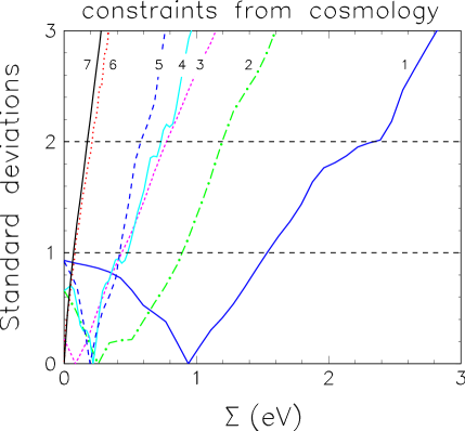
Figure 2: Constraints placed by different cosmological data sets (1,…,7) on the sum of neutrino masses $\Sigma$, in terms of standard deviations from the best fit in each case.

The above cases provide a sufficiently rich list of cosmological data combinations, with increasingly strong constraints on $\Sigma$. In particular, Fig. 2 shows the constraints on $\Sigma$ for each case of our analysis, in terms of standard deviations from the best fit of $\Sigma$. None of these curves shows evidence for neutrino mass at $>1\sigma$, indicating that current cosmological data can only set upper bounds on $\Sigma$. The bounds tend to scale linearly for the richest data sets (e.g., for the cases 5, 6, and 7).

Table 2: Input cosmological data sets for seven representative cases considered in this work, together with their $2\sigma$ (95% C.L.) constraints on the sum of neutrino masses $\Sigma$.

Case	Cosmological data set	$\Sigma$ bound ($2\sigma$)
1	WMAP	$<2.3$ eV
2	WMAP + SDSS	$<1.2$ eV
3	WMAP + SDSS + SNRiess + HST + BBN	$<0.78$ eV
4	CMB + LSS + SNAstier	$<0.75$ eV
5	CMB + LSS + SNAstier + BAO	$<0.58$ eV
6	CMB + LSS + SNAstier + Ly-$\alpha$	$<0.21$ eV
7	CMB + LSS + SNAstier + BAO + Ly-$\alpha$	$<0.17$ eV

Table II summarizes the bounds on $\Sigma$ derived from our analysis in numerical form (at the $2\sigma$ level). Such bounds are in agreement with previous results in similar recent analyses which include WMAP and other data, whenever a comparison is possible WMAP3 ; Seljak:2006bg ; goobar ; fukugita ; raffelt ; cirelli ; pastor , and we can derive the following conclusions:

• As already shown in WMAP3 and fukugita , the WMAP data alone, in the framework of cosmological models we are considering, are able to constrain $\Sigma\lesssim 2$ eV at $95\%$ C.L.. This limit, which relyes on a single high-quality dataset, should be considered as the most conservative.

• Inclusions of galaxy clustering and SN-Ia data can, as already pointed out in the literature (see e.g. fogli ; pastor and references therein), further constrain the results. The datasets used in the cases $2$, $3$, $4$ and $5$ contain different galaxy clustering and supernovae data and thus test the impact of possible different systematics. Such cases provide, respectively, constraints of $\Sigma<1.2$ eV, $\Sigma<0.78$ eV, $\Sigma<0.75$ eV and $\Sigma<0.58$ eV at $95\%$ C.L., respectively. These results are in reasonable agreement with the findings of, e.g., WMAP3 but are slightly weaker than those presented in goobar (case $5$ in particular), probably as a consequence of the different data analysis method. Just to mention few differences, in goobar the likelihood analysis is based on a database of models while we adopt Markov Chains. Moreover goobar includes variations in the equations of state parameter $w$ and running of the spectral index, while here we consider only models with $w=-1$ and no running. Non-standard models with a large negative running of the spectral index or with $w>-1$ prefer smaller neutrino masses when compared with observations. Finally, goobar uses the same bias parameter for the SLOAN and 2dF surveys while the two may be different.

• Including SDSS Ly-$\alpha$ data in cases $6$ and $7$ (as in Seljak:2006bg ) greatly improves the constraints on $\Sigma$ up to $\Sigma<0.21$eV and $\Sigma<0.17$eV ($95\%$ C.L.). The latter is stronger than the one reported in goobar , since we are using the updated SDSS Ly-$\alpha$ dataset of Seljak:2006bg . This constraint has important consequences for our analyses, especially when compared with the $m_{\beta\beta}$ claim. However, we remark that the bounds on the linear density fluctuations obtained from the SDSS Ly-$\alpha$ dataset are derived from measurement of the Ly-$\alpha$ flux power spectrum $P_{F}(k)$ after a long inversion process, which involves numerical simulations and marginalization over the several parameters of the Ly-$\alpha$ model. The strongest limit in case 7 should therefore be considered as the less conservative.

As we can see, cosmology seems to provide the best constraints available on absolute neutrino masses. However, sub-eV constraints can be placed only when we consider a combination of multiple datasets. It is therefore important to check the degree of compatibility between the datasets. A possible way to make such check and to better understand, at the same time, the data preference for small values of $\Sigma$, is to consider a joint analysis of $\Sigma$ and of the so-called $\sigma_{8}$ parameter, which represents the expected linear root mean square (rms) amplitude of matter fluctuations in spheres of radius $R=8h^{-1}$ Mpc.

Let us briefly remind that the linear (rms) mass fluctuations in spheres of radius $R$ are usually expressed throught their power spectrum $P(k)$ in Fourier space (see e.g. bondszalay ):

$$\sigma^{2}(R)=\int_{0}^{\infty}{dk\over k}\,4\pi k^{3}P(k)W^{2}(kR)\ ,$$ (16)

where $W(x)=3(\sin x-x\cos x)/x^{3}$ is the top-hat window function, and the mass enclosed in the sphere is $M=4\pi\rho_{0}R^{3}/3$, with $\rho_{0}$ denoting the background mass density of the universe. The matter power spectrum $P(k)$ is fully determined once the cosmological model and the corresponding parameters are defined. The effect of massive neutrinos is to reduce the amplitude of the power spectrum $P(k)$ on free streaming scales and, therefore, to reduce the value of $\sigma_{8}$. The neutrino free-streaming process introduces indeed an additional length scale in the power spectrum related to the median neutrino Fermi-Dirac speed $v_{\rm med}$ by $k_{fs}^{2}=4\pi G\rho/v^{2}_{\rm med}\propto\Sigma h$. For $k<k_{fs}$, the density perturbation in the neutrinos grows in the matter-dominated era while decays for $k>k_{fs}$. It is possible to show (see e.g. tegmax ) that for wavenumbers smaller than $k_{fs}$ the power specrum is damped by a factor

$$P(k;\Sigma)/P(k;0)\approx e^{-0.087(\Sigma/{\Omega_{m}h^{2}})}\ ,$$ (17)

where $\Omega_{m}$ is the total matter density. Therefore, in general, we expect that the larger $\Sigma$ the smaller $\sigma_{8}$ (or vice versa), namely, that these two parameters are partly degenerate, with negative correlations. If $\sigma_{8}$ is determined in some way, the degeneracy is “broken” and $\Sigma$ can be better constrained.

The value of $\sigma_{8}$ can be derived either in an indirect way, i.e., by first determining the cosmological model and by then considering the possible values of the allowed $P(k)$, or in a more direct way, i.e., by measuring the amount of galaxy clustering on $\sim 8$ Mpc scales. Since CMB observations provide an indirect determination of $\sigma_{8}$, it is important to check if this determination is compatible with the other, more direct, measurements made throught galaxy clustering. An incompatibility between the two datasets, with, for example, a low value preferred by CMB data vs a high value preferred by clustering data, would lead to a formally very strong (but practically unreliable) constraint on $\Sigma$ (see also WMAP3 ).

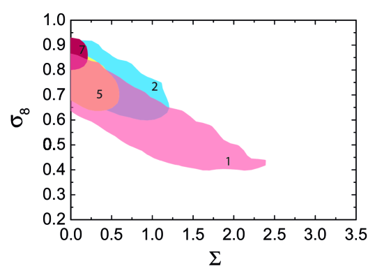
Figure 3: Joint $2\sigma$ constraints on the $(\sigma_{8},\,\Sigma)$ parameters (95% C.L. for $N_{\mathrm{DF}}=1$) derived from four representative cosmological data sets (1, 2, 5, and 7, as listed in Table II).

Fig. 3 shows the results of our joint analysis of the $(\sigma_{8},\,\Sigma)$ parameters, in terms of $2\sigma$ contours ($\Delta\chi^{2}=4$ for one degree of frreedom) for four representative cosmological data sets (1, 2, 5, and 7), chosen among the seven sets studied in this work (see Table II). In case 1 (WMAP only), the degeneracy and anticorrelation between the two parameters is evident. The addition of galaxy clustering and Ly-$\alpha$ tend to break the degeneracy by selecting increasingly smaller ranges for $\sigma_{8}$. It turns out that such additional data tend to prefer $\sigma_{8}$ in the “higher part” of the range allowed by WMAP only, so that the upper bound on $\Sigma$ is pushed to lower values. Should future data hypothetically invert such trend (i.e., the current preference for “high” values of $\sigma_{8}$), the upper bounds on $\Sigma$ would be somewhat relaxed. In any case, the different combinations of current cosmological data in Fig. 3 appear to be in relatively good agreement with each other, with significant overlap of the different $2\sigma$ regions—a reassuring consistency check.

V Global analyses: Results for various input data sets

In this section we discuss the global analysis of all neutrino oscillation and non-oscillation data, with particular attention to the (in)compatibility and combination (at $2\sigma$ level) of the various cosmological data sets (numbered as $1,\,2,\dots 7$ in Table 2) with the $0\nu 2\beta$ signal claim of Kl04 . First we examine the most conservative case where a combination is possible (case $1^{+}$ in Sec. V A), then we discuss the worst case where the combination is forbidden at $\gg 2\sigma$ (case 7 in Sec. V B), and finally we make an overview of the results for all possible intermediate cases considered in this work (Sec. V C).

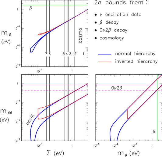
Figure 4: Superposition of $2\sigma$ constraints (95% C.L. for $N_{\mathrm{DF}}$=1) placed by $\beta$, $0\nu 2\beta$, oscillation, and cosmological neutrino data in the three 2-dimensional projections of the $(m_{\beta},\,m_{\beta\beta},\,\Sigma)$ parameter space. Cosmological constraints are labelled as in Table 2 for the seven input data sets. The $0\nu 2\beta$ lower limit on $m_{\beta\beta}$ from the claim in Kl04 is indicated as a horizontal dashed line.

The results discussed in more detail in the following sections can be qualitatively understood through Fig. 4, which—following the previous work fogli —shows the three orthogonal projections of the regions separately allowed at $2\sigma$ level in the $(m_{\beta},\,m_{\beta\beta},\,\Sigma)$ parameter space by: (a) neutrino oscillation data (slanted bands for normal and inverted hierarchy); (b) the seven cosmological data sets (numbered lines with “cosmo” label); (c) single $\beta$ decay searches (lines with $\beta$ label); and (d) $0\nu 2\beta$ decay limits (lines with $0\nu 2\beta$ label). In the latter case, the lower limit from the claim in Kl04 is shown as a dashed line to remind that, formally, it may be accepted or not. In Fig. 4 the various bounds are simply superposed, while real combinations of data are performed in the following sections. Note that the global combinations can alter the bounds from separate data sets: e.g., the global upper bounds on $\Sigma$ may be slightly different from those placed by cosmological data only, while lower bounds on $\Sigma$ (not placed at all by current cosmological data) arise when the oscillation data (i.e., the evidence for nonzero neutrino mass) is included.

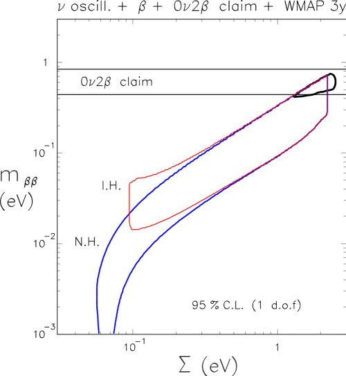
Figure 5: Comparison (at $2\sigma$) between the regions preferred by the $0\nu 2\beta$ signal claim (horizontal band) and by all $\nu$ oscillation data plus $\beta$ and WMAP-3y data (slanted bands) for normal (NH) and inverted (IH) hierarchy, in the plane ($m_{\beta\beta},\Sigma$). The combination of all such data (thick slanted “wedge” in the upper right corner of the plot) corresponds to “Case $1^{+}$” in the text.

V.1 Case with WMAP-3y data and the $0\nu 2\beta$ claim

The most conservative choice for the cosmological input is to rely only upon WMAP 3y data (case 1 in Table 2). In this case, the upper bound on $\Sigma$ is relatively weak ($\sim 2$ eV), and the “slanted band” allowed by the combination of oscillation and cosmological data in Fig. 4 can reach the horizontal band allowed by the claimed $0\nu 2\beta$ signal Kl04 , and a global combination of all data becomes possible. Figure 5 shows in more detail this situation in the relevant plane $(m_{\beta\beta},\Sigma)$, where the global combination (from a full $\chi^{2}$ analysis) yields a “wedge shaped” allowed region around $\Sigma\sim 2$ eV and $m_{\beta\beta}\sim\mathrm{few}\times 10^{-1}$ eV. This case will be labelled “$1^{+}$” in the following (meaning: cosmological data set 1, plus $0\nu 2\beta$ claim).

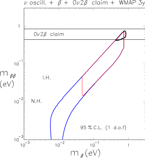
Figure 6: As in Fig. 5, but in the plane $(m_{\beta\beta},m_{\beta}$).

For the relatively high $\nu$ masses implied by the above $1^{+}$ case, the Mainz+Troitsk bound on $m_{\beta}$, included in the fit, slightly tightens the global constraints in the upper part of the wedge-shaped solution in Fig. 5 (this is the only such case). Not surprisingly, if the global combination dubbed “1+” were correct, a positive discovery of $m_{\beta}$ should be “around the corner,” just below the Mainz+Troitsk bound. For this reason, we find it useful to represent in Fig. 6 the same case $1^{+}$, but in the plane $(m_{\beta\beta},m_{\beta})$. A signal in the range $m_{\beta}\sim\mathrm{few}\times 10^{-1}$ eV is clearly expected, and could be found in the next-generation Karksruhe Tritium Neutrino Experiment (KATRIN) katrin , which should take data in the next decade.

V.2 Case with all cosmological data but without the $0\nu 2\beta$ claim

The most “aggressive” limit on $\Sigma$ is placed by all cosmological data (case 7 in Table 2), assuming that their combination is correct and that there are no hidden systematics. In this case, the upper limit on $\Sigma$ is so tight ($\sim 0.2$ eV), that no combination is possible with the $0\nu 2\beta$ claim at face value. The incompatibility is evident in Fig. 7, which shows how far are the regions allowed by oscillation and cosmological neutrino data for both normal and inverted hierarchy (confined in the lower left corner) and the $0\nu 2\beta$ claim (horizontal band). However, one should not be tempted to say that “cosmological data rule out the $0\nu 2\beta$ claim,” for at least three reasons: 1) such claim can only be (dis)proved by another $0\nu 2\beta$ experiment with greater sensitivity; 2) the $0\nu 2\beta$ signal might be due to new physics beyond light Majorana neutrinos; 3) independently of the correctness of the $0\nu 2\beta$ claim, cosmological bounds on neutrino masses should be taken with a grain of salt, given the many systematic uncertainties that typically affect astrophysical data, and given our persistent ignorance about two main ingredients of the standard cosmological model (dark matter and dark energy).

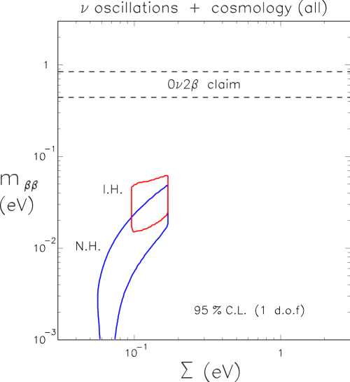
Figure 7: Comparison (at $2\sigma$ level) between the regions allowed by the $0\nu 2\beta$ signal claim (horizontal band) and by neutrino oscillation data plus all cosmological data (slanted bands) for normal (NH) and inverted (IH) hierarchy, in the plane ($m_{\beta\beta},\Sigma$). In this case, $\beta$ decay data constraints are not relevant, and oscillation plus cosmological data cannot be combined with the $0\nu 2\beta$ decay claim. This situation corresponds to “Case 7” in the text.

V.3 Overview of all cases

From a glance at Fig. 4, it appears that the $0\nu 2\beta$ claim is formally compatible (at $2\sigma$) with oscillation data plus cosmological bounds only if the latter include just WMAP-3y data (most conservative case 1). In this case, the global combination dubbed as $1^{+}$ in Sec. V A becomes possible. In all other cases, a combination would be formally possible only by stretching (some of) the errors at (much) more than $2\sigma$ — an attempt not pursued in this work. Therefore, except for the case $1^{+}$ already examined, we consider the possibility that the $0\nu 2\beta$ claim is wrong (i.e., that it provides an upper bound only), and combine oscillation data with all cosmological datasets (1,…,7) in either normal and inverted hierarchy.

Table 3: Allowed ranges at 95% C.L. ($2\sigma$) for the observables ($m_{\beta},\,m_{\beta\beta},\,\Sigma$), as derived from the global analysis of neutrino oscillation and non-oscillation data. The cases labeled from 1 to 7 (with either normal or inverted hierarchy) include the seven cosmological input data sets discussed in Sec. IV, with the $0\nu 2\beta$ decay claim Kl04 treated as a one-sided (upper) limit on $m_{\beta\beta}$. Only in the case $1^{+}$ we fully include the $0\nu 2\beta$ decay claim in the global combination (the hierarchy being irrelevant in such case). See the text for details.

Case	Hierarchy	$m_{\beta}$ (eV)	$m_{\beta\beta}$ (eV)	$\Sigma$ (eV)
$1^{+}$	Any	$[0.42,\,0.84]$	$[0.42,\,0.75]$	$[1.3,\,2.5]$
1	Normal	$[0.0057,\,0.69]$	$[0,\,0.66]$	$[0.056,\,2.1]$
2		$[0.0057,\,0.39]$	$[0,\,0.38]$	$[0.056,\,1.2]$
3		$[0.0057,\,0.25]$	$[0,\,0.24]$	$[0.056,\,0.75]$
4		$[0.0057,\,0.24]$	$[0,\,0.23]$	$[0.056,\,0.72]$
5		$[0.0057,\,0.18]$	$[0,\,0.18]$	$[0.056,\,0.56]$
6		$[0.0057,\,0.063]$	$[0,\,0.061]$	$[0.056,\,0.20]$
7		$[0.0057,\,0.050]$	$[0,\,0.048]$	$[0.056,\,0.17]$
1	Inverted	$[0.047,\,0.69]$	$[0.015,\,0.66]$	$[0.095,\,2.1]$
2		$[0.047,\,0.39]$	$[0.015,\,0.38]$	$[0.095,\,1.2]$
3		$[0.047,\,0.25]$	$[0.015,\,0.24]$	$[0.095,\,0.75]$
4		$[0.047,\,0.24]$	$[0.015,\,0.23]$	$[0.095,\,0.72]$
5		$[0.047,\,0.18]$	$[0.015,\,0.18]$	$[0.095,\,0.56]$
6		$[0.047,\,0.075]$	$[0.015,\,0.073]$	$[0.095,\,0.20]$
7		$[0.047,\,0.064]$	$[0.015,\,0.062]$	$[0.095,\,0.17]$

The results of such exercise are summarized in Table 3, in terms of $2\sigma$ allowed ranges for the three relevant observables $(m_{\beta},m_{\beta\beta},\Sigma)$. Such ranges may be useful to gauge the sensitivity required by future experiments, in order to explore the currently allowed parameter space. E.g., the $\beta$-decay experiment KATRIN, with an estimated sensitivity down to $\sim 0.2$ eV katrin , can fully test case $1^{+}$ in Table 3, may test a fraction of the parameter space up to case 4, but it cannot access cases 5, 6, and 7, which will necessarily require new $\beta$-decay detection techniques to probe the $O(0.1$–$0.01)$ eV range for $m_{\beta}$. Analogously, in order to significantly test the various cases in Table 3, cosmological data might need to reach a $2\sigma$ accuracy of about $\sim 0.1$ eV on $\Sigma$ (in the global fit), which may be feasible in the future pastor ; on the other hand, $0\nu 2\beta$ experiments might need to push their sensitivity down to $O(0.1)$ eV or even to $O(0.01)$ eV, which is quite challenging Elli . Cosmological data seems thus to be in a relatively good position to run the absolute neutrino mass race.

VI Implications for future $0\nu 2\beta$ decay searches

Concerning $0\nu 2\beta$ experiments, we have shown in Table 3 the expected ranges for the “canonical” parameter $m_{\beta\beta}$ in various cases. However, in practice, the experimentalists measure or constrain decay half lives ($T^{0\nu}_{1/2}$) rather than effective Majorana masses ($m_{\beta\beta}$). Indeed, some confusion arises in the literature when the sensitivity of different $0\nu 2\beta$ experiments is compared in terms of $m_{\beta\beta}$, but the nuclear matrix elements are not homogeneous, or they are not calculated within the same theoretical framework. Therefore, we think it is useful to present also more “practical” predictions for half lives $T^{0\nu}_{1/2}$ in different nuclei, by using one and the same theoretical nuclear model faessler with well-defined uncertainties (i.e., by using the matrix elements $C_{mm}$ as summarized in Table 1).

More precisely, the $m_{\beta\beta}$ ranges estimated in Table 3, together with the theoretical input values (and errors) for the nuclear matrix elements $C_{mm}$ reported in Table 1, are used to estimate the expected $2\sigma$ ranges for the $0\nu 2\beta$ half lives $T^{0\nu}_{1/2}$ in different nuclei through Equation (13). As previously remarked, the linear form of this equation makes it easier to propagate the uncertainties affecting $C_{mm}$ and $m_{\beta\beta}$. As a result, we obtain in Table 4 the $2\sigma$ ranges for the half-lives $T^{0\nu}_{1/2}$ of several candidate nuclei, for all cases ($1^{+},\,1,\,2,\dots,7$) previously considered in Sec. V.

Table 4: Allowed ranges at 95% C.L. ($2\sigma$) for the $0\nu 2\beta$ decay half-lives $T^{0\nu}_{1/2}$ of various candidate nuclei, for the same cases as in Table 3. The $T^{0\nu}_{1/2}$ ranges are derived from the relation $T^{0\nu}_{1/2}=m^{2}_{e}/(m^{2}_{\beta\beta}\,C_{mm})$, by using the $C_{mm}$ and $m_{\beta\beta}$ input from Table 1 and Table 3, respectively. The shorthand notation X.Y$e$ZW means $T^{0\nu}_{1/2}=\mathrm{X.Y}\times 10^{\mathrm{ZW}}$ yr. For the sake of comparison, in the last row we list existing experimental lower limits on $T^{0\nu}_{1/2}$ (at 90% C.L.), as taken from the recent compilations in Elli ; barabash .

Case	Hierarchy	${}^{76}\mathrm{Ge}$	${}^{82}\mathrm{Se}$	${}^{100}\mathrm{Mo}$	${}^{116}\mathrm{Cd}$	${}^{128}\mathrm{Te}$	${}^{130}\mathrm{Te}$	${}^{136}\mathrm{Xe}$
$1^{+}$	Any	$[1.0e25,\,3.5e25]$	$[2.9e24,\,1.1e25]$	$[5.4e24,\,2.3e25]$	$[3.4e24,\,1.7e25]$	$[7.2e25,\,4.2e26]$	$[3.2e24,\,1.9e25]$	$[5.2e24,\,8.7e25]$
1	Normal	$[1.1e25,\,\infty]$	$[3.0e24,\,\infty]$	$[5.1e24,\,\infty]$	$[3.2e24,\,\infty]$	$[6.5e25,\,\infty]$	$[2.9e24,\,\infty]$	$[4.3e24,\,\infty]$
2		$[3.3e25,\,\infty]$	$[8.9e24,\,\infty]$	$[1.5e25,\,\infty]$	$[9.5e24,\,\infty]$	$[1.9e26,\,\infty]$	$[8.7e24,\,\infty]$	$[1.3e25,\,\infty]$
3		$[8.3e25,\,\infty]$	$[2.2e25,\,\infty]$	$[3.9e25,\,\infty]$	$[2.4e25,\,\infty]$	$[4.9e26,\,\infty]$	$[2.2e25,\,\infty]$	$[3.2e25,\,\infty]$
4		$[9.1e25,\,\infty]$	$[2.5e25,\,\infty]$	$[4.3e25,\,\infty]$	$[2.6e25,\,\infty]$	$[5.4e26,\,\infty]$	$[2.4e25,\,\infty]$	$[3.5e25,\,\infty]$
5		$[1.4e26,\,\infty]$	$[3.9e25,\,\infty]$	$[6.8e25,\,\infty]$	$[4.2e25,\,\infty]$	$[8.5e26,\,\infty]$	$[3.2e25,\,\infty]$	$[5.6e25,\,\infty]$
6		$[1.3e27,\,\infty]$	$[3.4e26,\,\infty]$	$[5.9e26,\,\infty]$	$[3.6e26,\,\infty]$	$[7.4e27,\,\infty]$	$[3.3e26,\,\infty]$	$[4.9e26,\,\infty]$
7		$[2.1e27,\,\infty]$	$[5.6e26,\,\infty]$	$[9.8e26,\,\infty]$	$[8.0e26,\,\infty]$	$[1.2e28,\,\infty]$	$[5.5e26,\,\infty]$	$[6.5e26,\,\infty]$
1	Inverted	$[1.1e25,\,3.3e28]$	$[3.0e24,\,1.1e28]$	$[5.1e24,\,2.5e28]$	$[3.2e24,\,1.8e28]$	$[6.5e25,\,4.7e29]$	$[2.9e24,\,2.2e28]$	$[4.3e25,\,1.1e29]$
2		$[3.3e25,\,3.3e28]$	$[8.9e24,\,1.1e28]$	$[1.5e25,\,2.5e28]$	$[9.5e24,\,1.8e28]$	$[1.9e26,\,4.7e29]$	$[8.7e24,\,2.2e28]$	$[1.3e24,\,1.1e29]$
3		$[8.3e25,\,3.3e28]$	$[2.2e25,\,1.1e28]$	$[3.9e25,\,2.5e28]$	$[2.4e25,\,1.8e28]$	$[4.9e26,\,4.7e29]$	$[2.2e25,\,2.2e28]$	$[3.2e25,\,1.1e29]$
4		$[9.1e25,\,3.3e28]$	$[2.5e25,\,1.1e28]$	$[4.3e25,\,2.5e28]$	$[2.6e25,\,1.8e28]$	$[5.4e26,\,4.7e29]$	$[2.4e25,\,2.2e28]$	$[3.5e25,\,1.1e29]$
5		$[1.4e26,\,3.3e28]$	$[3.9e25,\,1.1e28]$	$[6.8e25,\,2.5e28]$	$[4.2e25,\,1.8e28]$	$[8.5e26,\,4.7e29]$	$[3.2e25,\,2.2e28]$	$[5.6e25,\,1.1e29]$
6		$[9.1e26,\,3.3e28]$	$[2.5e26,\,1.1e28]$	$[4.3e26,\,2.5e28]$	$[2.6e26,\,1.8e28]$	$[5.4e27,\,4.7e29]$	$[2.4e26,\,2.2e28]$	$[3.5e26,\,1.1e29]$
7		$[1.2e27,\,3.3e28]$	$[3.1e26,\,1.1e28]$	$[5.4e26,\,2.5e28]$	$[3.3e26,\,1.8e28]$	$[6.8e27,\,4.7e29]$	$[3.0e26,\,2.2e28]$	$[4.5e26,\,1.1e29]$
Limits (90% C.L.)		$\gtrsim 1.2e25$	$>2.1e23$	$>5.8e23$	$>1.7e23$	$>7.7e24$	$>2.2e24$	$>4.5e23$

The last row in Table 4 shows the current experimental limits on the various half lives, as taken from the recent compilations Elli ; barabash . It can be appreciated that, except for ⁷⁶Ge and ¹³⁰Te, current limits must be improved by about one order of magnitude (at least) in order to probe any of the cases in Table 1. Even for the most promising nuclei (⁷⁶Ge and ¹³⁰Te), however, an experimental improvement by a factor of a few in the $T^{0\nu}_{1/2}$ limits can only allow to probe the most optimistic case $1^{+}$, and a fraction of the cases 1 and 2. Probing the other cases ($3,\dots,7$) will require (much) more than an order-of-magnitude improvement with respect to current $0\nu 2\beta$ limits. It is thus very important to invest a great effort in future neutrinoless double beta decay experiments with increasing sensitivity to longer lifetimes, in order to match the typical expectations from current neutrino oscillation and cosmological data.

VII Conclusions

Building on previous work fogli and on updated experimental input, we have revisited the phenomenological constraints applicable to three observables sensitive to absolute neutrino masses: The effective neutrino mass in single beta decay $(m_{\beta})$; the effective Majorana neutrino mass in neutrinoless double beta decay $(m_{\beta\beta})$; and the sum of neutrino masses in cosmology $(\Sigma)$. In particular, we have included the constraints coming from the first MINOS results MINOS and from the WMAP-3y data WMAP3 , as well as other relevant cosmological data and priors. We have found that the largest neutrino mass squared difference $\Delta m^{2}$ is now determined with a 15% accuracy (at $2\sigma$). We have also examined the upper bounds on the sum of neutrino masses $\Sigma$, as well as their correlations with the matter power spectrum normalization parameter $\sigma_{8}$. The bounds range from $\Sigma\lesssim 2$ eV (WMAP-3y data only) to $\Sigma\lesssim 0.2$ eV (all cosmological data) at $2\sigma$, in agreement with previous studies. Finally, for various possible combination of data sets, we have revisited the (in)compatibility between current $\Sigma$ and $m_{\beta\beta}$ constraints, and have derived quantitative predictions for single and double beta-decay observables, which can be useful to evaluate the sensitivity required by present and future experiments in order to explore the currently allowed parameter space.

- (1) Review of Particle Physics, S. Eidelman et al., Phys. Lett. B 592, 1 (2004).
- (2) G. L. Fogli, E. Lisi, A. Marrone, and A. Palazzo, Prog. Part. Nucl. Phys. 57, 742 (2006).
- (3) A. Strumia and F. Vissani, hep-ph/0606054.
- (4) G. L. Fogli, E. Lisi, A. Marrone, A. Melchiorri, A. Palazzo, P. Serra, and J. Silk, Phys. Rev. D 70, 113003 (2004).
- (5) MINOS Collaboration, D.G. Michael et al., hep-ex/0607088.
- (6) WMAP Collaboration, D. N. Spergel et al., astro-ph/0603449.
- (7) U. Seljak, A. Slosar, and P. McDonald, astro-ph/0604335.
- (8) A. Goobar, S. Hannestad, E. Mortsell and H. Tu, astro-ph/0602155.
- (9) M. Fukugita, K. Ichikawa, M. Kawasaki, and O. Lahav, Phys. Rev. D 74, 027302 (2006).
- (10) S. Hannestad and G. G. Raffelt, astro-ph/0607101.
- (11) M. Cirelli and A. Strumia, astro-ph/0607086.
- (12) J. Lesgourgues and S. Pastor, Phys. Rept. 429, 307 (2006).
- (13) H. V. Klapdor-Kleingrothaus, I. V. Krivosheina, A. Dietz, and O. Chkvorets, Phys. Lett. B 586, 198 (2004).
- (14) V. Gavrin, talk at Neutrino 2006, XXII International Conference on Neutrino Physics and Astrophysics (Santa Fe, New Mexico, USA, 2006). Website: neutrinosantafe06.com
- (15) CHOOZ Collaboration, M. Apollonio et al., Eur. Phys. J. C 27, 331 (2003).
- (16) Super-Kamiokande Collaboration, J. Hosaka et al., hep-ex/0604011.
- (17) K2K Collaboration, M. H. Ahn et al., hep-ex/0606032.
- (18) K. Eitel, in the Proceedings of Neutrino 2004, 21st International Conference on Neutrino Physics and Astrophysics (Paris, France, 2004), edited by J. Dumarchez, Th. Patzak, and F. Vannucci, Nucl. Phys. B (Proc. Suppl.) 143, 197 (2005).
- (19) S. R. Elliott and J. Engel, J. Phys. G 30, R183 (2004).
- (20) H. V. Klapdor-Kleingrothaus, talk at SNOW 2006, 2nd Scandinavian Neutrino Workshop (Stockholm, Sweden, 2006). Website: www.theophys.kth.se/snow2006
- (21) V. A. Rodin, A. Faessler, F. Simkovic, and P. Vogel, Nucl. Phys. A 766, 107 (2006).
- (22) A. Lewis and S. Bridle, Phys. Rev. D 66, 103511 (2002). Software available at the website: cosmologist.info
- (23) WMAP Collaboration, G. Hinshaw et al., astro-ph/0603451.
- (24) LAMBDA website: lambda.gsfc.nasa.gov
- (25) M. Tegmark et al., Astrophys. J. 606, 702 (2004).
- (26) W. L. Freedman et al., Astrophys. J. 553, 47 (2001).
- (27) A. G. Riess et al., Astrophys. J. 665R, 607 (2004).
- (28) A. C. S. Readhead et al., Astrophys. J. 609, 498 (2004).
- (29) C. Dickinson et al., Mon. Not. Roy. Astron. Soc. 353, 732 (2004).
- (30) C. L. Kuo et al., American Astronomical Society Meeting, Vol. 201 (2002).
- (31) C. J. MacTavish et al., astro-ph/0507503.
- (32) S. Cole et al., Mon. Not. Roy. Astron. Soc. 362, 505 (2005).
- (33) P. Astier et al., Astron. Astrophys. 447, 31 (2006).
- (34) D. J. Eisenstein et al., Astrophys. J. 633, 560 (2005).
- (35) P. McDonald et al., Astrophys. J. Suppl. 163, 80 (2006).
- (36) P. McDonald et al., Astrophys. J. 635, 761 (2005).
- (37) S. Dodelson, A. Melchiorri, and A. Slosar, Phys. Rev. Lett. 97, 04301 (2006).
- (38) J. R. Bond and A. S. Szalay, Astrophys. J. 274, 443 (1983).
- (39) M. Tegmark, Phys. Scripta T121, 153 (2005) [hep-ph/0503257].
- (40) See talks by P. Doe and F. Glück at Neutrino 2006 gavrin .
- (41) A. S. Barabash, hep-ex/0602037; partly updated in the talk at Neutrino 2006 gavrin .