Quasi-Particle Description of Strongly Interacting Matter: Towards a Foundation

Abstract

We confront our quasi-particle model for the equation of state of strongly interacting matter with recent first-principle QCD calculations. In particular, we test its applicability at finite baryon densities by comparing with Taylor expansion coefficients of the pressure for two quark flavours. We outline a chain of approximations starting from the $\Phi$-functional approach to QCD which motivates the quasi-particle picture.

1 Introduction

In the last years, great progress has been made in the numerical evaluation of QCD thermodynamics from first principles (dubbed lattice QCD) even for finite chemical potentials Allton1 ; FK ; Fodor ; deForcrand ; Lombardo . While various perturbative expansions Arnold95 ; Zhai95 ; Kajantie03 ; Vuorinen ; Ipp04 fail in describing thermodynamics of strongly interacting matter in the vicinity of $T_{c}$ ($T_{c}$ being the (pseudo-) critical temperature of deconfinement and chiral symmetry restauration), different phenomenological approaches exist which aim to reproduce the non-perturbative behaviour. For instance, models based on quasi-particle pictures with effectively modified properties due to strong interactions are successful in describing lattice QCD results Levai ; Schneider ; Letessier ; Rebhan ; Thaler ; Ivanov ; Peshier . Analytical approaches with a rigorous link to QCD (cf. Rischke for a survey) such as direct HTL resummation Andersen ; Andersen02b or $\Phi$-functional approach Blaizot ; Blaizot01 ; Blaizot02 formulated in terms of dressed propagators are successful in describing lattice QCD on temperatures $T\gtrsim 2T_{c}$.

It is the aim of the present paper to show the successful applicability of our quasi-particle model (QPM) for describing lattice QCD results and to motivate the model starting from the $\Phi$-functional approach to QCD. In section 2, we review the QPM and compare with recent lattice QCD results for pressure and entropy density. In section 3, a possible chain of approximations is outlined starting from QCD within the $\Phi$-functional approximation scheme which motivates our formulation of QCD thermodynamics in terms of quasi-particle excitations. We summarize our results in section 4.

2 QPM and Comparison with Lattice QCD

In our model, the pressure $p$ for $N_{f}=2$ light quark flavours in thermal equilibrium as function of temperature $T$ and one chemical potential $\mu_{q}$ ($\mu_{g}=0$) reads

$$p(T,\mu_{q})=\sum_{a=q,g}p_{a}-B(T,\mu_{q})\,,$$ (1)

where $p_{a}=d_{a}/(6\pi^{2})\int_{0}^{\infty}dkk^{4}\left(f_{a}^{+}+f_{a}^{-}\right)/\omega_{a}$ denote the partial pressures of quarks ($q$) and transverse gluons ($g$). Here, $d_{q}=2N_{f}N_{c}$, $d_{g}=N_{c}^{2}-1$, $N_{c}=3$, and $f_{a}^{\pm}=(\exp([\omega_{a}\mp\mu_{a}]/T)+S_{a})^{-1}$ with $S_{q}=1$ for fermions and $S_{g}=-1$ for bosons. $B(T,\mu_{q})$ is determined from thermodynamic self-consistency and the stationarity of $p$ under functional variation with respect to the self-energies, $\delta p/\delta\Pi_{a}=0$ Gorenstein . $\Pi_{a}$ enter the quasi-particle dispersion relations $\omega_{a}$ being approximated by asymptotic mass shell expressions near the light cone, $\omega_{a}=\sqrt{k^{2}+\Pi_{a}}$. We employ the asymptotic expressions of the gauge independent hard thermal (dense) loop self-energies LeBellac96 . Finite bare quark masses $m_{0;q}$ as used in lattice simulations can be implemented following Pisarski .

By replacing the running coupling $g^{2}$ in $\Pi_{a}$ with an effective coupling $G^{2}(T,\mu_{q})$, non-perturbative effects in the vicinity of $T_{c}$ are accomodated. In this way, we achieve enough flexibility to describe lattice QCD results. We parametrize $G^{2}(T,\mu_{q}=0)$ (cf. Blu05 for details) by

$$G^{2}(T,\mu_{q}=0)=\left\{\begin{array}[]{l}G^{2}_{\rm(2)}(\xi(T)),\,T\geq T_{c},\\[8.53581pt] G^{2}_{\rm(2)}(\xi(T_{c}))+b(1-\frac{T}{T_{c}}),\,T<T_{c},\end{array}\right.$$ (2)

where $G^{2}_{\rm(2)}$ is the relevant part of the 2-loop running coupling and $\xi(T)=\lambda(T-T_{s})/T_{c}$ contains a scale parameter $\lambda$ and an infrared regulator $T_{s}$. The effective coupling $G^{2}$ for arbitrary $T$ and $\mu_{q}$ can be found by solving a quasi-linear partial differential equation which follows from Maxwell’s relation,

$$a_{\mu_{q}}\frac{\partial G^{2}}{\partial\mu_{q}}+a_{T}\frac{\partial G^{2}}{\partial T}=b\,.$$ (3)

The coefficients in (3) explicitly read (neglecting for simplicity additional contributions stemming from $T$-dependent bare quark masses as employed in lattice simulations)

$$a_{T} = {\rm I_{1}}\frac{C_{f}}{4}\left(T^{2}+\frac{\mu_{q}^{2}}{\pi^{2}}\right)\,,$$ (4)

$$a_{\mu_{q}} = -{\rm I_{2}}\frac{C_{f}}{4}\left(T^{2}+\frac{\mu_{q}^{2}}{\pi^{2}}\right)$$

$$-{\rm I_{3}}\left(\left[N_{c}+\frac{N_{f}}{2}\right]\frac{T^{2}}{6}+\frac{N_{c}N_{f}}{12\pi^{2}}\mu_{q}^{2}\right)\,,$$

$$b = -{\rm I_{1}}\frac{C_{f}}{2}TG^{2}+{\rm I_{2}}\frac{C_{f}}{2}\frac{\mu_{q}}{\pi^{2}}G^{2}$$

$$+{\rm I_{3}}\frac{N_{c}N_{f}}{6\pi^{2}}\mu_{q}G^{2}\,.$$

Here,

$${\rm I_{1}} = \frac{d_{q}}{4\pi^{2}T}\int_{0}^{\infty}dk\frac{k^{2}}{\omega_{q}}\bigg{(}e^{\omega_{q}^{+}/T}(f_{q}^{-})^{2}-e^{\omega_{q}^{-}/T}(f_{q}^{+})^{2}\bigg{)},$$ (7)

$${\rm I_{2}} = \frac{d_{q}}{2\pi^{2}T}\int_{0}^{\infty}dk\frac{k^{2}}{\omega_{q}}\bigg{(}f_{q}^{+}-\frac{L_{q}f_{q}^{+}}{\omega_{q}}\bigg{[}\frac{1}{\omega_{q}}+\frac{e^{\omega_{q}^{-}/T}}{T}f_{q}^{+}\bigg{]}$$

$$+\frac{\mu_{q}}{2T}e^{\omega_{q}^{-}/T}(f_{q}^{+})^{2}+f_{q}^{-}-\frac{L_{q}f_{q}^{-}}{\omega_{q}}\bigg{[}\frac{1}{\omega_{q}}+\frac{e^{\omega_{q}^{+}/T}}{T}f_{q}^{-}\bigg{]}$$

$$-\frac{\mu_{q}}{2T}e^{\omega_{q}^{+}/T}(f_{q}^{-})^{2}\bigg{)},$$

$${\rm I_{3}} = \frac{d_{g}}{\pi^{2}T}\int_{0}^{\infty}dk\frac{k^{2}}{\omega_{g}}f_{g}\left(1-\frac{L_{g}}{\omega_{g}}\left[\frac{1}{\omega_{g}}+\frac{e^{\omega_{g}/T}}{T}f_{g}\right]\right)$$ (9)

with $f_{g}^{\pm}\equiv f_{g}$, $\omega_{q}^{\pm}=\omega_{q}\pm\mu_{q}$, $L_{a}=2k^{2}/3+\Pi_{a}/2$ and $C_{f}=(N_{c}^{2}-1)/2N_{c}$.

Entropy density $s=\partial p/\partial T=\sum_{a=q,g}s_{a}$ and net density $n=n_{q}=\partial p/\partial\mu_{q}$ follow from (1) as

$$s_{a} = \frac{d_{a}}{2\pi^{2}T}\int_{0}^{\infty}dkk^{2}\bigg{(}\frac{\frac{4}{3}k^{2}+\Pi_{a}}{\omega_{a}}\left[f_{a}^{+}+f_{a}^{-}\right]$$

$$-\mu_{a}\left[f_{a}^{+}-f_{a}^{-}\right]\bigg{)}\,,$$

$$n_{q} = \frac{d_{q}}{2\pi^{2}}\int_{0}^{\infty}dkk^{2}\left[f_{q}^{+}-f_{q}^{-}\right]\,.$$ (11)

In Fig. 1, we exhibit QPM results for $p$ and $s$ at $\mu_{q}=0$ compared with lattice QCD results for different numbers of quark flavours Kar1 ; Kar2 .

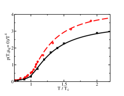
Figure 1: Comparison of our QPM with lattice QCD results (symbols) for $p(T,\mu_{q}=0)/T^{4}$ (upper panel) and $s(T,\mu_{q}=0)/T^{3}$ (lower panel) as functions of $T/T_{c}$ for $N_{f}=2$ (squares) Kar1 and $N_{f}=2+1$ ($\mu_{s}=0$) (circles) Kar1 ; Kar2 . Raw lattice QCD data are continuum extrapolated as advocated in Kar1 ; Kar3 . QPM parameters: $\lambda=4.4$, $T_{s}=0.67T_{c}$, $b=344.4$, $B(T_{c})=0.31T_{c}^{4}$ with $T_{c}=175$ MeV for $N_{f}=2$ and $\lambda=7.6$, $T_{s}=0.80T_{c}$, $b=348.7$, $B(T_{c})=0.52T_{c}^{4}$ with $T_{c}=170$ MeV for $N_{f}=2+1$.

Recently, the decomposition of $p$ into a Taylor series in powers of ($\mu_{q}/T$) for small $\mu_{q}$ was studied in lattice QCD All05 ,

$$p(T,\mu_{q})=T^{4}\sum_{n=0}^{\infty}c_{n}(T)\left(\frac{\mu_{q}}{T}\right)^{n}\,.$$ (12)

The expansion coefficients $c_{n}(T)$, vanishing for odd $n$ and depending only on temperature $T$, follow using (1) from

$$c_{n}(T)=\left.\frac{1}{n!}\frac{\partial^{n}(p/T^{4})}{\partial(\mu_{q}/T)^{n}}\right|_{\mu_{q}=0}\,.$$ (13)

$c_{n}(T)$ depend on $G^{2}$ and its derivatives with respect to $\mu_{q}$ at $\mu_{q}=0$, thus testing (3). Furthermore, net density $n$ can also be decomposed into a Taylor series at small $\mu_{q}$ with expansion coefficients $c_{n}(T)$. Therefore, the higher order coefficients $c_{2,4,6}(T)$ serve for a more direct test of the applicability of our model at finite $\mu_{q}$. In Fig. 2, we compare $c_{2,4,6}(T)$ evaluated from (13) with lattice QCD results for $N_{f}=2$ All05 . In particular, the pronounced structures in the vicinity of $T_{c}$ are fairly well reproduced (cf. Blu05 ).

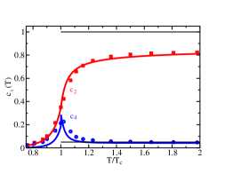
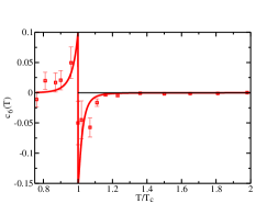
Figure 2: Comparison of our QPM with lattice QCD results (symbols) All05 for $c_{2,4}(T)$ (upper panel) and $c_{6}(T)$ (lower panel) as functions of $T/T_{c}$ for $N_{f}=2$. QPM parameters: $\lambda=12.0$, $T_{s}=0.87T_{c}$, $b=426.1$, with $T_{c}=175$ MeV. The horizontal lines at $T\geq T_{c}$ depict the corresponding Stefan-Boltzmann values highlighting the effects of strong interaction near $T_{c}$.

3 Foundations of the QPM

Having successfully reproduced first-principle lattice QCD results, it would be desirable to establish contact between our ad hoc introduced QPM in section 2 and QCD as the fundamental microscopic gauge field theory of strong interactions. In order to motivate our quasi-particle model, we present a possible chain of approximations starting from QCD within the $\Phi$-functional approach following the pioneering work Blaizot ; Blaizot01 ; Blaizot02 . We concentrate on entropy density $s$ and net density $n$, as they turn out to possess a simple structure supporting the picture of quasi-particle excitations. Other thermodynamic quantities such as pressure $p$ or energy density $e$ are determined from $s$ and $n$. Although rather strong assumptions become mandatory in the derivation, one should be aware of the remarkable success of our QPM in describing lattice QCD results.

In the $\Phi$-functional approach Luttinger60 ; Baym62 to QCD, the thermodynamic potential $\Omega=-T\ln Z$ can be expressed as a functional of dressed propagators of gluons $D$, quarks $S$ and Faddeev-Popov ghost fields $G$,

$$\frac{\Omega[D,S,G]}{T}= \frac{1}{2}{\rm Tr}[\ln D^{-1}\!-\!\Pi D]-{\rm Tr}[\ln S^{-1}\!-\!\Sigma S]$$

$$-{\rm Tr}[\ln G^{-1}-\Xi G]+\Phi[D,S,G]\,.$$

Here, ghost field contributions compensate for possible unphysical degrees of freedom in the gluon propagator. While the propagators in (3) depend on the specific gauge, $\Omega=-pV$ must be gauge independent. For convenience, we choose the Coulomb gauge in the following in which ghost fields do not propagate and the gluon propagator consists only of the physical transverse and longitudinal modes. The functional $\Phi[D,S]$ is given by the infinite sum of all $2\,$-particle irreducible skeleton diagrams constructed from $D$ and $S$.

The self-energies are related to the dressed propagators by Dyson’s equations

$$\Pi[D]=D^{-1}-D_{0}^{-1}\,\,,\,\,\Sigma[S]=S^{-1}-S_{0}^{-1}\,,$$ (15)

where $D_{0}$ and $S_{0}$ represent the bare propagators of gluon and quark fields, respectively. Demanding the stationarity of $\Omega$ under functional variation with respect to the dressed propagators Lee60

$$\left.\frac{\delta\Omega[D,S]}{\delta D}\right|_{D_{0}}=\left.\frac{\delta\Omega[D,S]}{\delta S}\right|_{S_{0}}=0\,,$$ (16)

the self-energies follow self-consistently by cutting a dressed propagator line in $\Phi$ resulting in the gap equations

$$\Pi=2\frac{\delta\Phi[D,S]}{\delta D}\,\,,\,\,\Sigma=-\frac{\delta\Phi[D,S]}{\delta S}\,.$$ (17)

The trace $"{\rm Tr}"$ in (3) has to be taken over all states of the relativistic many-particle system. In the imaginary time formalism it can be rewritten in the form ${\rm Tr}\rightarrow{\rm tr}\,\beta VT\sum_{n=-\infty}^{+\infty}\int d^{3}k/(2\pi)^{3}$. Here, $V$ is the volume of the system, $\beta=1/T$ and $"{\rm tr}"$ denotes the remaining trace over occuring discrete indices including colour, flavour, Lorentz or spinor indices. Introducing the four-momentum $k^{\nu}=(\omega,\vec{k})=(i\omega_{n},\vec{k})$, the sums have to be taken over the Matsubara frequencies $\omega_{n}=2n\pi T$ (or $(2n+1)\pi T-i\mu$) for gluons (or quarks). They can be evaluated by using standard contour integration techniques in the complex $\omega$-plane LeBellac96 ; Kapusta89 wrapping up the poles of the propagators. Expressing the analytic propagators in terms of their spectral densities $\rho$, one can define

$$\rho_{D(S)}(\omega,|\vec{k}|)=2\lim_{\epsilon\rightarrow 0}{\rm Im}\,D(S)(\omega+i\epsilon,|\vec{k}|)$$ (18)

for real $\omega$. Similarly, the imaginary parts of functions of the analytic propagators obeying the same pole structures can be defined. Hence, $\Omega$ reads with retarded propagators $D$ and $S$ depending on $\omega$ and $k=|\vec{k}|$

$$\frac{\Omega[D,S]}{V}= {\rm tr}\int\frac{d^{4}k}{(2\pi)^{4}}n(\omega)\,{\rm Im}[\ln D^{-1}-\Pi\,D]$$

$$+2{\rm tr}\int\frac{d^{4}k}{(2\pi)^{4}}f(\omega)\,{\rm Im}[\ln S^{-1}-\Sigma\,S]+\frac{T}{V}\Phi[D,S]\,,$$

where $\int d^{4}k=\int d^{3}k\int d\omega$, and $n(\omega)=(e^{\beta\omega}-1)^{-1}$ ($f(\omega)=(e^{\beta(\omega-\mu)}+1)^{-1}$) denotes the statistical distribution function for gluons (quarks with chemical potential $\mu$).

Due to the stationarity property (16), entropy density $s=-\partial(\Omega/V)/\partial T$ and net density $n=-\partial(\Omega/V)/\partial\mu$ contain only explicit temperature and chemical potential derivatives of $n(\omega)$ and $f(\omega)$, although the propagators in (3) depend implicitly on $T$ and $\mu$ through their spectral densities. Using ${\rm Im}\,(\Pi D)={\rm Im}\,\Pi\,{\rm Re}\,D+{\rm Re}\,\Pi\,{\rm Im}\,D$, one finds for the entropy density $s=s_{g}+s_{q}+s^{\prime}$ with

$$s_{g}=-{\rm tr}\int\frac{d^{4}k}{(2\pi)^{4}}\frac{\partial n(\omega)}{\partial T}[{\rm Im}\ln D^{-1}-{\rm Im}\,\Pi\,{\rm Re}D]\,,$$ (20)

$$s_{q}=-2{\rm tr}\int\frac{d^{4}k}{(2\pi)^{4}}\frac{\partial f(\omega)}{\partial T}[{\rm Im}\ln S^{-1}-{\rm Im}\,\Sigma\,{\rm Re}S]\,,$$ (21)

$$s^{\prime} =-\left.\frac{\partial(\frac{T}{V}\Phi[D,S])}{\partial T}\right|_{D,S}+2{\rm tr}\int\frac{d^{4}k}{(2\pi)^{4}}\frac{\partial f(\omega)}{\partial T}{\rm Re}\Sigma\,{\rm Im}S$$ (22)

$$+{\rm tr}\int\frac{d^{4}k}{(2\pi)^{4}}\frac{\partial n(\omega)}{\partial T}{\rm Re}\Pi\,{\rm Im}D\,.$$

Similarly, for the net density one finds $n=n_{q}+n^{\prime}$ with

$$n_{q} = -2{\rm tr}\int\frac{d^{4}k}{(2\pi)^{4}}\frac{\partial f(\omega)}{\partial\mu}[{\rm Im}\ln S^{-1}-{\rm Im}\,\Sigma\,{\rm Re}S],$$ (23)

$$n^{\prime} = 2{\rm tr}\int\frac{d^{4}k}{(2\pi)^{4}}\frac{\partial f(\omega)}{\partial\mu}{\rm Re}\Sigma\,{\rm Im}S$$

$$-\left.\frac{\partial(\frac{T}{V}\Phi[D,S])}{\partial\mu}\right|_{D,S}\,.$$

While the sum integrals in $\Omega$ (3) contain ultraviolet divergencies which must be regularized, the expressions for $s_{g}$, $s_{q}$ and $n_{q}$ in (20, 21) and (23) are manifestly ultraviolet convergent because the derivatives of the statistical distribution functions vanish for $\omega\rightarrow\pm\infty$. In addition, introducing real multiplicative renormalization factors for propagators and self-energies, these factors simply drop out of $s$ and $n$.

Self-consistent (or $\Phi$-derivable) approximation schemes preserve the stationarity property (16) of $\Omega$ when truncating the infinite sum in $\Phi$ at a specific loop order while corresponding self-energies and propagators are self-consistently evaluated from (17) and Dyson’s equations. Nevertheless, self-consistency does not guarantee gauge invariance which is an important issue in truncated expansion schemes. In fact, by modifying propagators but leaving vertices unaffected Ward identities are violated.

We consider $\Phi$ at 2 - loop order in the following which is diagrammatically represented by Peshier01

$$\vspace{.5cm}\Phi=\frac{1}{12}\,\,\,\parbox{71.13188pt}{\immediate\ignorespaces\immediate\ignorespaces\immediate\ignorespaces\immediate\ignorespaces\immediate\ignorespaces{\f@ynmf:phis\char 1\relax}\ignorespaces\immediate\ignorespaces\immediate\ignorespaces\immediate\ignorespaces\immediate\ignorespaces\immediate\ignorespaces\immediate\ignorespaces\immediate\ignorespaces\immediate\ignorespaces\immediate\ignorespaces\immediate\ignorespaces\immediate\ignorespaces\immediate\ignorespaces \immediate\ignorespaces}+\,\frac{1}{8}\,\,\,\parbox{71.13188pt}{\immediate\ignorespaces\immediate\ignorespaces\immediate\ignorespaces\immediate\ignorespaces\immediate\ignorespaces{\f@ynmf:phis\char 2\relax}\ignorespaces\immediate\ignorespaces\immediate\ignorespaces\immediate\ignorespaces\immediate\ignorespaces\immediate\ignorespaces\immediate\ignorespaces\immediate\ignorespaces\immediate\ignorespaces\immediate\ignorespaces\immediate\ignorespaces\immediate\ignorespaces\immediate\ignorespaces\immediate\ignorespaces \immediate\ignorespaces}-\,\,\frac{1}{2}\parbox{56.9055pt}{\immediate\ignorespaces\immediate\ignorespaces\immediate\ignorespaces\immediate\ignorespaces\immediate\ignorespaces{\f@ynmf:phis\char 3\relax}\ignorespaces\immediate\ignorespaces\immediate\ignorespaces\immediate\ignorespaces\immediate\ignorespaces\immediate\ignorespaces\immediate\ignorespaces\immediate\ignorespaces\immediate\ignorespaces\immediate\ignorespaces\immediate\ignorespaces\immediate\ignorespaces\immediate\ignorespaces \immediate\ignorespaces}.$$ (25)

Here, wiggly (solid) lines denote gluons (quarks). The self-consistent self-energies are accordingly

$$\vspace{.5cm}\Pi=\frac{1}{2}\,\,\parbox{71.13188pt}{\immediate\ignorespaces\immediate\ignorespaces\immediate\ignorespaces\immediate\ignorespaces\immediate\ignorespaces{\f@ynmf:selfs\char 1\relax}\ignorespaces\immediate\ignorespaces\immediate\ignorespaces\immediate\ignorespaces\immediate\ignorespaces\immediate\ignorespaces\immediate\ignorespaces\immediate\ignorespaces\immediate\ignorespaces\immediate\ignorespaces\immediate\ignorespaces \immediate\ignorespaces}+\frac{1}{2}\,\,\parbox{71.13188pt}{\immediate\ignorespaces\immediate\ignorespaces\immediate\ignorespaces\immediate\ignorespaces\immediate\ignorespaces{\f@ynmf:selfs\char 2\relax}\ignorespaces\immediate\ignorespaces\immediate\ignorespaces\immediate\ignorespaces\immediate\ignorespaces\immediate\ignorespaces\immediate\ignorespaces\immediate\ignorespaces\immediate\ignorespaces\immediate\ignorespaces\immediate\ignorespaces \immediate\ignorespaces}-\,\parbox{71.13188pt}{\immediate\ignorespaces\immediate\ignorespaces\immediate\ignorespaces\immediate\ignorespaces\immediate\ignorespaces{\f@ynmf:selfs\char 3\relax}\ignorespaces\immediate\ignorespaces\immediate\ignorespaces\immediate\ignorespaces\immediate\ignorespaces\immediate\ignorespaces\immediate\ignorespaces\immediate\ignorespaces\immediate\ignorespaces\immediate\ignorespaces \immediate\ignorespaces},$$ (26)

$$\vspace{.3cm}\Sigma=\,\,\parbox{71.13188pt}{\immediate\ignorespaces\immediate\ignorespaces\immediate\ignorespaces\immediate\ignorespaces\immediate\ignorespaces{\f@ynmf:newself\char 1\relax}\ignorespaces\immediate\ignorespaces\immediate\ignorespaces\immediate\ignorespaces\immediate\ignorespaces\immediate\ignorespaces\immediate\ignorespaces\immediate\ignorespaces\immediate\ignorespaces\immediate\ignorespaces\immediate\ignorespaces \immediate\ignorespaces}.$$ (27)

Although vertex corrections can be implemented self-consistently Freedman78 , they turn out to be negligible at 2 - loop order in $\Phi$ Blaizot01 . In addition, $s^{\prime}=n^{\prime}=0$ is found for the residual contributions of entropy density and net density in (22) and (3) at 2 - loop order Blaizot01 . This topological feature being related to (17) has also been observed in massless $\Phi^{4}$-theory Peshier01 ; Peshier98a and in QED Vanderheyden .

Concentrating on the gluonic contribution $s_{g}$, (20) can be rewritten by using the identity

$${\rm Im}[\ln D^{-1}(\omega,k)]=-\pi{\rm sgn}(\omega)\,\Theta(-{\rm Re}D^{-1}(\omega,k))$$ (28)

$$+\arctan\left(\frac{{\rm Im}\Pi(\omega,k)}{{\rm Re}D^{-1}(\omega,k)}\right)$$

where $-\pi/2<\arctan x<\pi/2$. Hence, $s_{g}$ can be decomposed into $s_{g}=s_{g,QP}+s_{g,LD}$ with

$$s_{g,QP} = {\rm tr}\int\frac{d^{3}k}{(2\pi)^{3}}\int\frac{d\omega}{2}\frac{\partial n(\omega)}{\partial T}{\rm sgn}(\omega)\,\Theta(-{\rm Re}D^{-1})\,,$$ (29)

$$s_{g,LD} = {\rm tr}\int\frac{d^{4}k}{(2\pi)^{4}}\frac{\partial n(\omega)}{\partial T}\bigg{\{}{\rm Im}\Pi\,{\rm Re}D$$

$$-\arctan\left(\frac{{\rm Im}\Pi}{{\rm Re}D^{-1}}\right)\bigg{\}}\,.$$

Here, (29) accounts for the contribution of dynamical quasi-particles to $s_{g}$ defined by the poles of $D$ and (3) represents the contribution from the continuum part of the spectral density associated with a cut below the light cone $|\omega|<k$ Pisarski ; Peshier04 representing Landau damping. Applying a similar identity for ${\rm Im}[\ln S^{-1}(\omega,k)]$, $s_{q}$ and $n_{q}$ in (21, 23) can be decomposed similarly into quasi-particle and Landau-damping contributions.

In Coulomb gauge, $D$ consists of a longitudinal and a transverse part, $D_{L}$ and $D_{T}$. Similarly, the (massless) quark propagator consists of two different branches with chirality either equal (positive energy states) or opposite (negative energy states) to helicity. By employing the gauge invariant hard thermal loop (HTL) expressions $\hat{\Pi}$ ($\hat{\Sigma}$) for the gluon (quark) self-energies in the following, one obtains gauge invariant approximations of $s$ and $n$. The HTL expressions read LeBellac96

$$\hat{\Pi}_{L}(\omega,k) = \hat{m}_{D}^{2}\left(1-\frac{\omega}{2k}\ln\frac{\omega+k}{\omega-k}\right),$$ (31)

$$\hat{\Pi}_{T}(\omega,k) = \frac{1}{2}\left(\hat{m}_{D}^{2}+\frac{\omega^{2}-k^{2}}{k^{2}}\hat{\Pi}_{L}(\omega,k)\right),$$ (32)

$$\hat{\Sigma}_{\pm}(\omega,k) = \frac{\hat{M}^{2}}{k}\left(1-\frac{\omega\mp k}{2k}\ln\frac{\omega+k}{\omega-k}\right),$$ (33)

with Debye screening mass (allowing, in general, for different chemical potentials $\mu_{i}$)

$$\hat{m}_{D}^{2}=\left([2N_{c}+N_{f}]T^{2}+N_{c}\sum_{i}\frac{\mu_{i}^{2}}{\pi^{2}}\right)\frac{g^{2}}{6}\,,$$ (34)

long-wavelength fermionic frequency

$$\hat{M}^{2}=\frac{N_{c}^{2}-1}{16N_{c}}\left(T^{2}+\frac{\mu_{i}^{2}}{\pi^{2}}\right)g^{2}\,,$$ (35)

and running coupling $g^{2}$. Although being derived originally for soft external momenta $\omega,k\sim gT\ll T$, they coincide on the light cone with complete 1-loop results Thoma as exhibited in Fig. 3. Finite

Figure 3: Comparison of HTL approximation (the nearly indistinguishable short and long dashed curves are for massless (32) (cf. Thoma ) and massive quarks, $m_{q}=0.4\,T$, as used in lattice calculations Kar1 ; Kar2 ; Kar3 ; All05 , respectively) with 1-loop results (solid curves for massive quarks) Kalashnikov of the scaled real part of the transverse gluon self-energy as function of $\omega/T$ for $k/T=0.1$, $0.5$ and $1$ from left to right. $N_{f}=2$, $\mu_{i}=0$. In the vicinity of the light cone $\omega=k$ (shaded regions), HTL results approximate 1-loop results fairly well even for $k\sim T$ which is the thermodynamically relevant part in momentum space but with decreasing agreement for increasing $k$.

quark masses, $m<T$, turn out to be negligible. The corresponding propagators are evaluated from Dyson’s equations.

For $k\sim T,\mu$ the poles of both, longitudinal gluon propagator as well as abnormal fermion branch have exponentially vanishing residues Pisarski giving only minor contributions to the thermodynamics. Therefore, we assume that these collective modes can be neglected in the following. Furthermore, being a severe approximation, we also neglect any imaginary parts of the self-energies, i. e. ${\rm Im}\hat{\Pi}_{T}={\rm Im}\hat{\Sigma}_{+}=0$. Then, the Landau damping contributions to $s_{g}$, $s_{q}$ and $n_{q}$ vanish. Finite width effects associated with imaginary parts of the self-energies are discussed by Peshier Peshier04 . Including Landau damping as well as the exponentially suppressed modes, it was shown in Rebhan that in this way some ambiguities arising when solving (3) can be eliminated.

Performing the $\omega$-integration in (29) (but now for $\hat{D}_{T}$), the only contributions stem from $\omega^{2}\geq\omega_{T}^{2}$ because of the $\Theta$-function, where $\omega_{T}$ is the positive solution of $\omega^{2}-k^{2}-\hat{\Pi}_{T}(\omega,k)=0$. Therefore, the $\omega$-integral in (29) reads

$$\int_{-\infty}^{\infty}\frac{d\omega}{2}\frac{\partial n(\omega)}{\partial T}{\rm sgn}(\omega)\,\Theta(-{\rm Re}\hat{D}_{T}^{-1})=$$ (36)

$$\int_{\infty}^{\omega_{T}}\frac{d\omega}{2}\left(\frac{\partial n(-\omega)}{\partial T}-\frac{\partial n(\omega)}{\partial T}\right)\,.$$

The remaining integration is performed through an integration by parts using $-\partial n(\omega)/\partial T=\partial n(-\omega)/\partial T=\partial\sigma(\omega)/\partial\omega$ for the spectral function $\sigma(\omega)=-n(\omega)\ln n(\omega)+\left(1+n(\omega)\right)\ln\left(1+n(\omega)\right)$. Taking the trace over polarization and colour degrees of freedom for the transverse gluon modes, one finds

$$s_{g,QP}=-2(N_{c}^{2}-1)\int\frac{d^{3}k}{(2\pi)^{3}}\bigg{(}\ln(1-e^{-\beta\omega_{T}})$$ (37)

$$-\frac{\beta\omega_{T}}{e^{\beta\omega_{T}}-1}\bigg{)}\,.$$

Similarly, $s_{q,QP}$ can be evaluated, where non-vanishing contributions to the $\omega$-integration stem from $\omega\geq\omega_{+}$. Here, $\omega_{+}$ is the solution of $\omega-k-\hat{\Sigma}_{+}(\omega,k)=0$ for the positive fermion branch. Using $-\partial f(\omega)/\partial T=\partial\sigma(\omega)/\partial\omega$ for the spectral function $\sigma(\omega)=-f(\omega)\ln f(\omega)-(1-f(\omega))\ln(1-f(\omega))$, the $\omega$-integral can be integrated by parts. Antiquarks are included by simply replacing $\mu\rightarrow-\mu$ in $f(\omega)$. Taking the trace over remaining spin, colour and flavour degrees of freedom, one finds

$$s_{q,QP} =2N_{c}N_{f}\int\frac{d^{3}k}{(2\pi)^{3}}\bigg{(}\ln(1+e^{-\beta(\omega_{+}-\mu)})$$

$$+\frac{\beta(\omega_{+}-\mu)}{e^{\beta(\omega_{+}-\mu)}+1}\bigg{)}$$

$$\quad\!+2N_{c}N_{f}\int\frac{d^{3}k}{(2\pi)^{3}}\bigg{(}\ln(1+e^{-\beta(\omega_{+}+\mu)})$$

$$+\frac{\beta(\omega_{+}+\mu)}{e^{\beta(\omega_{+}+\mu)}+1}\bigg{)}\,.$$

$s_{g,QP}$ and $s_{q,QP}$ in (37, 3) represent entropy density contributions of non-interacting quasi-particles with quantum numbers of transverse gluons (quarks) and dispersion relation $\omega_{T}$ ($\omega_{+}$).

Correspondingly, $n_{q,QP}$ is evaluated using $-\partial f(\omega)/\partial\mu=\partial f(\omega)/\partial\omega$. Adding antiquarks by $\mu\rightarrow-\mu$ in $f(\omega)$ (note, now $\partial f(\omega)/\partial\mu=\partial f(\omega)/\partial\omega$) and taking the trace, $n_{q,QP}$ reads

$$n_{q,QP} =2N_{c}N_{f}\int\frac{d^{3}k}{(2\pi)^{3}}\bigg{(}\frac{1}{e^{\beta(\omega_{+}-\mu)}+1}-\frac{1}{e^{\beta(\omega_{+}+\mu)}+1}\bigg{)}\,.$$ (39)

Finally, we approximate the quasi-particle dispersion relations by the asymptotic mass shell expressions near the light cone, thus neglecting any momentum or energy dependence of the self-energies. We employ $\omega_{T}\rightarrow\omega_{g}=\sqrt{k^{2}+\Pi_{g}}$ and $\omega_{+}\rightarrow\omega_{q}=\sqrt{k^{2}+\Pi_{q}}$ as in section 2 with asymptotic masses $\Pi_{g}=\hat{m}_{D}^{2}/2$ and $\Pi_{q}=2\hat{M}^{2}$, considering only one chemical potential $\mu_{i}=\mu_{q}$ ($\sum_{i}\mu_{i}^{2}\rightarrow N_{f}\mu_{q}^{2}$). Integrating the logarithmic terms in (37, 3) by parts (note that (39) already obeys the desired form), one exactly recovers expressions (2, 11) of our QPM, where the replacement of $g^{2}$ by $G^{2}$ remains as phenomenological procedure on top of the listed ”approximations”.

4 Conclusions

In summary, motivated by the successful reproduction of available results of QCD thermodynamics, we attempted a collection of necessary steps to establish the link of our employed quasi-particle model to QCD. Quite severe assumptions had to be made. Even with these, resulting in the formal structure of our model, an additional and crucial point is the parametrization of the effective coupling. While allowing for an accurate two-parameter fit of many different lattice QCD results, it requires a foundation. In this respect, we refer to the work in Shuryak , where the authors argue that the pure quasi-particle excitations, deduced from a preliminary study of the poles of quark and gluon propagators Petreczky , are too heavy to saturate the pressure delivered from lattice calculations, e. g. Kar2 , i. e. signalling the necessity of including additional degrees of freedom. Further systematic studies of the relevant degrees of freedom in the strongly coupled quark-gluon medium near $T_{c}$ are highly awaited to have some guidance.

An additional issue is the chiral extrapolation. The quark masses of $0.4\,T$ employed in the here analyzed lattice simulations correspond to unphysically heavy pions with $m_{\pi}\sim 770$ MeV. In the 1-loop and HTL gluon self-energy considered here, such a finite quark mass has a tiny (negligible) impact. A more rigorous treatment of finite quark mass effects must be accomplished to arrive at a suitable chiral extrapolation.

Acknowledgements. M.B. would like to thank the organizers of Hot Quarks 2006 for the invitation to a stimulating workshop. This work is supported by BMBF 06 DR 121, GSI and Helmholtz association VI. We thank J.P. Blaizot, F. Karsch, E. Laermann and A. Peshier for fruitful discussions.

References

- (1) C.R. Allton et al., Phys. Rev. D 66, 074507 (2002)
- (2) Z. Fodor, S.D. Katz, Phys. Lett. B 534, 87 (2002)
- (3) Z. Fodor, S.D. Katz, K.K. Szabo, Phys. Lett. B 568, 73 (2003)
- (4) P. de Forcrand, O. Philipsen, Nucl. Phys. B 642, 290 (2002); Nucl. Phys. B 673, 170 (2003)
- (5) M. D’Elia, M.-P. Lombardo, Phys. Rev. D 67, 014505 (2003); Phys. Rev. D 70, 074509 (2004)
- (6) P. Arnold, C. Zhai, Phys. Rev. D 51, 1906 (1995)
- (7) C. Zhai, B. Kastening, Phys. Rev. D 52, 7232 (1995)
- (8) K. Kajantie et al., Phys. Rev. D 67, 105008 (2003)
- (9) A. Vuorinen, Phys. Rev. D 67, 074032 (2003); Phys. Rev. D 68, 054017 (2003)
- (10) A. Ipp, A. Rebhan, A. Vuorinen, Phys. Rev. D 69, 077901 (2004)
- (11) P. Levai, U. Heinz, Phys. Rev. C 57, 1879 (1998)
- (12) R.A. Schneider, W. Weise, Phys. Rev. C 64, 055210 (2001)
- (13) J. Letessier, J. Rafelski, Phys. Rev. C 67, 031902 (2003)
- (14) A. Rebhan, P. Romatschke, Phys. Rev. D 68, 025022 (2003)
- (15) M.A. Thaler, R.A. Schneider, W. Weise, Phys. Rev. C 69, 035210 (2004)
- (16) Yu.B. Ivanov, V.V. Skokov, V.D. Toneev, Phys. Rev. D 71, 014005 (2005)
- (17) A. Peshier et al., Phys. Lett. B337, 235 (1994); Phys. Rev. D 54, 2399 (1996); A. Peshier, B. Kämpfer, G. Soff, Phys. Rev. C 61, 045203 (2000); Phys. Rev. D 66, 094003 (2002)
- (18) D.H. Rischke, Prog. Part. Nucl. Phys. 52, 197 (2004)
- (19) J.O. Andersen, E. Braaten, M. Strickland, Phys. Rev. Lett. 83, 2139 (1999); Phys. Rev. D 61, 014017 (1999); Phys. Rev. D 61, 074016 (2000)
- (20) J.O. Andersen, M. Strickland, Phys. Rev. D 66, 105001 (2002)
- (21) J.P. Blaizot, E. Iancu, A. Rebhan, Phys. Rev. Lett. 83, 2906 (1999); Phys. Lett. B 470, 181 (1999); Phys. Lett. B 523, 143 (2001); in Quark Gluon Plasma, edited by R.C. Hwa (World Scientific, Singapore, 2003)
- (22) J.P. Blaizot, E. Iancu, A. Rebhan, Phys. Rev. D 63, 065003 (2001)
- (23) J.P. Blaizot, E. Iancu, Phys. Rept. 359, 355 (2002)
- (24) M.I. Gorenstein, S.N. Yang, Phys. Rev. D 52, 5206 (1995)
- (25) M. Le Bellac, Thermal field theory (Cambridge University Press, Cambridge, England, 1996)
- (26) R.D. Pisarski, Physica A 158, 146 (1989); Nucl. Phys. A498, 423c (1989)
- (27) M. Bluhm, B. Kämpfer, G. Soff, Phys. Lett. B 620, 131 (2005)
- (28) F. Karsch, E. Laermann, A. Peikert, Phys. Lett. B 478, 447 (2000)
- (29) F. Karsch, K. Redlich, A. Tawfik, Eur. Phys. J. C 29 (2003) 549
- (30) F. Karsch, Nucl. Phys. Proc. Suppl. 83, 14 (2000)
- (31) C.R. Allton et al., Phys. Rev. D 68, 014507 (2003); Phys. Rev. D 71, 054508 (2005)
- (32) J.M. Luttinger, J.C. Ward, Phys. Rev. 118, 1417 (1960)
- (33) G. Baym, Phys. Rev. 127, 1391 (1962)
- (34) T.D. Lee, C.N. Yang, Phys. Rev. 117, 22 (1960)
- (35) J.I. Kapusta, Finite-temperature field theory (Cambridge University Press, Cambridge, England, 1989)
- (36) A. Peshier, Phys. Rev. D 63, 105004 (2001); Nucl. Phys. A 702, 128 (2002)
- (37) B.A. Freedman, L. McLerran, Phys. Rev. D 16, 1130 (1978)
- (38) A. Peshier et al., Eur. Phys. Lett. 43, 381 (1998)
- (39) B. Vanderheyden, G. Baym, J. Stat. Phys. 93, 843 (1998); in Progress in Nonequilibrium Green’s functions, edited by M. Bonitz (World Scientific, Singapore 2000)
- (40) A. Peshier, Phys. Rev. D 70, 034016 (2004); J. Phys. G 31 371 (2005)
- (41) A. Peshier, K. Schertler, M.H. Thoma, Annals Phys. 266, 162 (1998)
- (42) O.K. Kalashnikov, Fortsch. Phys. 32, 525 (1984)
- (43) E.V. Shuryak, I. Zahed, Phys. Rev. D 70, 054507 (2004)
- (44) P. Petreczky et al., Nucl. Phys. Proc. Suppl. 106, 513 (2002)