Abstract

We study the relation of vector Proca field formalism and antisymmetric tensor field formalism for spin-one resonances in the context of the large $N_{C}$ inspired chiral resonance Lagrangian systematically up to the order $O(p^{6})$ and give a transparent prescription for the transition from vector to antisymmetric tensor Lagrangian and vice versa. We also discuss the possibility to describe the spin-one resonances using an alternative “mixed” first order formalism, which includes both types of fields simultaneously, and compare this one with the former two. We also briefly comment on the compatibility of the above lagrangian formalisms with the high-energy constraints for concrete $VVP$ correlator.

1 Introduction

The low energy effective theory of QCD, known as chiral perturbation theory ($\chi PT$)[1, 2, 3], has made a considerable progress recently by means of the extension of the calculational scheme to the order $O(p^{6})$ (a comprehensive review of the recent calculations and the most important achievements can be found in [4] together with a complete list of references). The successful solution of the technical problems and increasing number of physical quantities computed at the next-to-next-to-leading order within the three-flavour expansion raised an issue of much more detailed knowledge of the free parameters (known as low-energy couplings (LECs)) of the $\chi PT$  Lagrangian ${\cal L}_{\chi}$,

$${\cal L}_{\chi}={\cal L}_{\chi}^{(2)}+{\cal L}_{\chi}^{(4)}+{\cal L}_{\chi}^{(6)},$$ (1)

in order to make contact of the higher precision $O(p^{6})$ calculations with phenomenology. The LECs, representing nonperturbative parameters of the underlying QCD dynamics associated with chiral symmetry breaking, are not uniquely determined from symmetry considerations only, and, at the order $O(p^{6})$, only few combinations of them are directly accessible from experimental data. The usual way of thinking about the actual values of LECs is to associate them with the physics of the low-lying resonances at the scale $\Lambda_{H}\sim 1GeV$ via chiral sum rules (for $O(p^{4})$ LECs listed e.g. in [2]). These relate the LECs to the low-energy expansion of the QCD correlators at zero momentum and exploit the information about the high-energy fall off of the correlators known from the operator product expansion (OPE). The corresponding spectral functions in the intermediate resonance region are either taken from experiment (see e.g. [5, 6]) or modelled using plausible theoretical assumptions (see e.g. [7, 8]). The considerations based on the large-$N_{C}$ expansion of QCD are particularly useful in such a type of reasoning [9]. In the limit $N_{C}\rightarrow\infty$, the correlators of quark bilinears can be calculated in terms of tree graphs within an effective theory containing infinite tower of weakly coupled narrow meson resonances with appropriate quantum numbers. The Lagrangian ${\cal L}_{\infty}$ of this effective theory (called chiral resonance Lagrangian) is not known from the first principles, however, it can be basically constructed on the symmetry grounds and its free parameters can be related to the phenomenology of the resonance sector. Up to the order $O(p^{6})$ it has the general form

$${\cal L}_{\infty} = {\cal L}_{GB}+{\cal L}_{res}$$ (2)

$$= {\cal L}_{GB}^{(2)}+{\cal L}_{GB}^{(4)}+{\cal L}_{GB}^{(6)}+{\cal L}_{res}^{(4)}+{\cal L}_{res}^{(6)}\,,$$

where ${\cal L}_{GB}=$ ${\cal L}_{GB}^{(2)}+{\cal L}_{GB}^{(4)}+{\cal L}_{GB}^{(6)}$ contains only the (pseudo)Goldstone bosons and ${\cal L}_{GB}^{(2n)}$ has the same form as the $O(p^{2n})$ $\chi PT$  Lagrangian ${\cal L}_{\chi}^{(2n)}$(cf. (1); the corresponding LECs are, however, different). ${\cal L}_{res}^{(4)}$ and ${\cal L}_{res}^{(6)}$ are the resonance Lagrangians of the chiral order $O(p^{4})$ and $O(p^{6})$ respectively. Integrating out the resonance fields from the chiral resonance Lagrangian and expanding to the given chiral order yields an effective $\chi PT$  Lagrangian ${\cal L}_{\chi}$ identified with (1) with LECs expressed in terms of the resonance parameters and the LECs from ${\cal L}_{GB}$. Schematically, up to the order $O(p^{6})$

$${\cal L}_{\chi} = {\cal L}_{GB}+{\cal L}_{\chi,\,res}$$ (3)

$$= {\cal L}_{GB}^{(2)}+{\cal L}_{GB}^{(4)}+{\cal L}_{GB}^{(6)}+{\cal L}_{\chi,\,res}^{(4)}+{\cal L}_{\chi,\,res}^{(6)}\,.$$

Here ${\cal L}_{\chi,\,res}^{(2n)}$ has the same form as ${\cal L}_{GB}^{(2n)}$ with LECs depending on the resonance masses and couplings of ${\cal L}_{res}={\cal L}_{res}^{(4)}+{\cal L}_{res}^{(6)}$. Though in principle ${\cal L}_{res}$ should contain infinite tower of resonance fields, it usually suffices to include only a finite number of them (corresponding to the lowest hadronic states in each channel) to saturate the LECs successfully, as it was shown in the seminal paper [10] for the $O(p^{4})$ LECs. Since then this idea has been often used in particular cases in order to estimate also the contribution of the $O(p^{6})$ LECs to various quantities calculated within the $O(p^{6})$ $\chi PT$. Quite recently, the first steps towards a systematic and consistent estimate of the $O(p^{6})$ LECs via resonance saturation have been made in [11, 12], where the general discussion of the method as well as the comparison of the results with experimental constraints from the observables of $\pi K$ scattering can be found.

However, the Lagrangian ${\cal L}_{\infty}$, given by (2), is not unique. The reason is that a general Lagrangian for spin-1 resonances can be formulated using various types of fields, the most common ones in this context are the vector Proca fields and antisymmetric tensor fields (i.e. the label $res\equiv V$ or $T$ in the above formulae), which both transform homogeneously under a nonlinear realization of the chiral symmetry. The equivalence of these two formulations of the resonance Lagrangian was studied in the past (cf. references [10, 21, 27, 28, 22, 29, 30]).

As pointed out in [22], there are several levels of equivalence of the various resonance Lagrangians. The first corresponds to the level of the chiral resonance Lagrangians ${\cal L}_{\infty}$. Complete equivalence here means equality of the physical observables (Green functions), calculated in the full chiral resonance theory, after the various coupling constants in one model are expressed in terms of the coupling constants of the other model. In other words, there exists a unique transformation connecting the coupling constants in both chiral resonance Lagrangians, which relates the results of both calculations. A weaker form of such an equivalence, the incomplete one, ensures equality of the observables modulo terms of the higher chiral order ($O(p^{8})$ in our case).

The second level compares the Lagrangians ${\cal L}_{res}$ only. It means equivalence of the contributions to the corresponding effective chiral Lagrangians ${\cal L}_{\chi,\,res}={\cal L}_{\chi,\,res}^{(4)}+{\cal L}_{\chi,\,res}^{(6)}$ obtained after integrating out the resonance fields. Again on this level one can distinguish two cases [22]. Strong equivalence is defined as the equality of contributions to the ${\cal L}_{\chi,\,res}$ in the sense that both formulations yield the same contributions to the effective chiral couplings when expressing the various parameters in one resonance Lagrangian ${\cal L}_{res}$ in terms of the parameters of the other one. Strong equivalence ensures therefore equality of the chiral expansion of the contribution from ${\cal L}_{res}$ to physical observables up to the order $O(p^{6})$. Weak equivalence means equality of the effective $O(p^{6})$ chiral Lagrangians ${\cal L}_{\chi,\,res}$ only when additional contact terms independent of the resonance fields of the form ${\cal L}_{GB}^{(4)}+{\cal L}_{GB}^{(6)}$ (with particularly adjusted LECs) are appended to one of the resonance Lagrangians.

The complete equivalence of ${\cal L}_{\infty}$ expressed in terms of vector and antisymmetric tensor fields, was first proved up to the order $O(p^{4})$ in Ref. [21] using the high-energy constraints to find the relation between the couplings in both approaches. More precisely, the general Lagrangian with antisymmetric tensor fields

$${\cal L}_{T,\infty}={\cal L}_{GB}^{(2)}+{\cal L}_{\,T}^{(4)}$$ (4)

was shown to be completely equivalent to vector field Lagrangian

$${\cal L}_{V,\infty}={\cal L}_{GB}^{(2)}+{\cal L}_{GB}^{(4)}+{\cal L}_{\,V}^{(6)}$$ (5)

with particular choice of ${\cal L}_{GB}^{(4)}$ and ${\cal L}_{\,V}^{(6)}$. Within the above classification, however, ${\cal L}_{\,T}^{(4)}$ and this particular ${\cal L}_{\,V}^{(6)}$ are only weakly equivalent, because the corresponding ${\cal L}_{\chi,\,T}^{(4)}$ and ${\cal L}_{\chi,\,V}^{(4)}$ differs by contact terms from ${\cal L}_{GB}^{(4)}$. These contact terms were found to be necessary to correct the possible wrong high-energy behaviour of certain observables calculated within the vector formalism. The role of such contact terms ensuring the positivity of the Hamiltonian was demonstrated in [27, 28], where also the proof of the above equivalence in the hamiltonian formalism was given. Later on the equivalence was proved using path integral methods in Ref. [29] (cf. also [23] for critical remarks) and in Ref. [30] (cf. also [24]).

With restriction to the anomalous sector of ${\cal L}_{\chi,\,res}$, the weak equivalence of ${\cal L}_{\,T}^{(4)}+{\cal L}_{\,T}^{(6)\,{\rm odd}}$ and ${\cal L}_{\,V}^{(6)}+{\cal L}_{\,V}^{(6){\rm odd}}$ was established [22] (where ${\cal L}_{\,T}^{(4)}$ and ${\cal L}_{\,V}^{(6)}$ were the same as in the previous case and ${\cal L}_{\,T}^{(6)\,{\rm odd}}$ and ${\cal L}_{\,V}^{(6){\rm odd}}$ were constructed according to the “minimal coupling” hypothesis), however, the complete equivalence was not studied.

In this paper, we try to enlarge the analysis of the equivalence of vector Proca field formalism and antisymmetric tensor formalism systematically up to the order $O(p^{6})$ and give a transparent prescription for the transition from vector to antisymmetric tensor Lagrangian and vice versa. We also study the possibility to describe the spin-one resonances using an alternative “mixed” first order formalism formulated in terms of both types of fields simultaneously and compare this one with the former two. We also briefly comment on the compatibility of the above lagrangian formalisms with the high-energy constraints for concrete QCD correlator.

The paper is organized as follows. In Section 2 we first fix our notation and briefly review the Proca field and antisymmetric tensor field formalisms. Section 3 is devoted to the detailed analysis of the equivalence of both approaches. As an explicit example of the various levels of equivalence and as an illustration of the transition prescription from antisymmetric tensor to vector form we use the $VVP$ correlator in Section 4. Alternative first order description of spin-one resonances is presented in Section 5, where also the relation to the former two approaches is clarified and illustrated using $VVP$ correlator. Brief summary is given is Section 6. Formal properties of the first order formalism, as well as some technical details are included in the Appendix A.

2 Basic concepts and notation

In what follows, we restrict our discussion only to one multiplet of the vector resonances, for definiteness we assume $1^{--}$ nonet. In this section we briefly review two standard possible representation of this particle states using Proca vector fields, which we denote generically $V$ $\equiv V_{\mu}^{a}$ and the antisymmetric tensor fields, for which we use the general symbol $R\equiv R_{\mu\nu}^{a}$. In what follows, in order to avoid cumbersome expressions, we shall systematically suppress both the Lorentz and group indices and use a condensed “dotted” and “bracket” notation for their respective contractions. Within this notation, we write for two generic four-vectors $A_{\mu}^{a}$ and $B_{\nu}^{b}$

$$(A\cdot B)\equiv A_{\mu}^{a}B^{a\mu}$$

and, more generally, whenever a dot appears between two tensors, it means contraction over the adjacent Lorentz indices. Also whenever two or more objects with group indices appear in a given sequence, we tacitly assume contraction of the adjacent group indices. Within this convention, e.g.

$$(V\cdot K\cdot V)\equiv V_{\mu}^{a}K^{ab\mu\nu}V_{\nu}^{b}\,.$$

For generic tensors we employ “$:$” for a pair of contracted antisymmetric indices, i.e.

$$R:J \equiv R_{\mu\nu}J^{\mu\nu}$$

$$R:J::RR \equiv R^{\mu\nu}J_{\mu\nu\,\,\alpha\beta\,\,\kappa\lambda}R^{\alpha\beta}R^{\kappa\lambda}\,.$$

We also mark by hat symbol an antisymmetrization, e.g. for a generic Lorentz rank two tensor $C_{\mu\nu}^{a\ldots}$ we write

$$\widehat{C}\equiv C_{\mu\nu}^{a\ldots}-C_{\nu\mu}^{a\ldots}$$

and generally for antisymmetrization of two adjacent Lorentz indices

$$\widehat{AB}\equiv A_{\ldots\mu}B_{\nu\ldots}-A_{\ldots\nu}B_{\mu\ldots}\,.$$

As an example of these rules, we can abbreviate $D_{\mu}^{ab}V_{\nu}^{b}-D_{\nu}^{ab}V_{\mu}^{b}$, where $V$ is the Proca field and $D\equiv D_{\mu}^{ab}$ is the usual covariant derivative as, $\widehat{DV}$.

2.1 Proca field formalism

Let us take into account just the interaction terms linear and quadratic in the resonance fields and write the Lagrangian for the vector-field representation in the following symbolic form

$${\cal L}_{V}=-\frac{1}{4}(\widehat{V}:\widehat{V})+\frac{1}{2}m^{2}(V\cdot V)+(J_{1}\cdot V)+(J_{2}:\widehat{V})+\frac{1}{2}(V\cdot K\cdot V)+(V\cdot J_{3}:\widehat{V})\,.$$ (6)

With a slight abuse of the above notation we have further introduced here $\widehat{V}=\widehat{DV}$ . Here and in what follows, we will often use for a generic external source built of chiral blocks a symbol $J_{i}$, where $i$ indicates a number of Lorentz indices.

The most general form of the Lagrangian (6) to lowest non-trivial order in the chiral expansion was first constructed in [31] and often used in the literature to estimate the $O(p^{6})$ low-energy constants (see e.g. in [8]). Explicit expressions for the external sources $J_{i}$ , $i=1,2,3$ and $K$ in terms of the usual basic chiral building blocs are given in the Appendix B. Here we only mention the chiral order of the sources

$$J_{1} = O(p^{3})\,,$$

$$J_{2} = O(p^{2})\,,$$

$$J_{3} = O(p)\,,$$

$$K = O(p^{2})\,.$$ (7)

Let us make several notes here. First, the interaction terms linear in the resonance fields start at $O(p^{3})$. This suggests to assign to the field $V_{\mu}$ the chiral order $O(p^{3})$, provided we are interested only in the resonance contributions to the low energy constant of the $O(p^{6})$ chiral Lagrangian. In this case we have the decomposition

$${\cal L}_{V}={\cal L}_{V}^{(6)}+{\cal L}_{V}^{(8)}\,,$$ (8)

where

$${\cal L}_{V}^{(6)} = \frac{1}{2}m^{2}(V\cdot V)+(J_{1}\cdot V)+(J_{2}:\widehat{V})\,,$$

$${\cal L}_{V}^{(8)} = -\frac{1}{4}(\widehat{V}:\widehat{V})+\frac{1}{2}(V\cdot K\cdot V)+(V\cdot J_{3}:\widehat{V})$$

and the corresponding effective $O(p^{6})$ chiral Lagrangian can be then obtained by integrating out the resonance field to the desired chiral order. Because the integration is gaussian, this effectively means inserting the solution of the equation of motion to the lowest non-trivial order $O(p^{3})$

$$V^{(3)}=-\frac{1}{m^{2}}\left(J_{1}-2D\cdot J_{2}\right)$$ (9)

in ${\cal L}_{V}^{(6)}$. The result is

$${\cal L}_{\chi,V}^{(6)} = -\frac{1}{2m^{2}}\left(\left(J_{1}-2D\cdot J_{2}\right)\cdot\left(J_{1}-2D\cdot J_{2}\right)\right)$$ (10)

$$= -\frac{1}{2m^{2}}\left(J_{1}\cdot J_{1}\right)+\frac{2}{m^{2}}\left(D\cdot J_{2}\cdot J_{1}\right)+\frac{2}{m^{2}}\left(D\cdot J_{2}\cdot J_{2}\cdot\overleftarrow{D}\right)$$

As pointed out in [21], the contributions to the $O(p^{4})$ LEC are not generated, unless extra contact terms are added to the Lagrangian. On the other hand, the interaction terms contained in the ${\cal L}_{V}^{(8)}$ give contributions only to the $O(p^{8})$ chiral Lagrangian and could be therefore ignored. Note also that, in principle, higher derivative terms as well as terms cubic in the resonance fields can be added to the Lagrangian, however (counting $V=O(p^{3})$), these are of higher chiral order (at least $O(p^{8})$) and are therefore irrelevant for our consideration. Nevertheless, both types of the additional terms mentioned above might be necessary in order to ensure the proper short-distance behaviour of certain Green functions dictated by OPE, cf. e.g. [21], [8].

Last note concerns the form of ${\cal L}_{V}^{(6)}$. Using integration by parts, which leads to the completely equivalent Lagrangian on the resonance level, one can of course get rid of the term $(J_{2}:\widehat{V})$ redefining $J_{1}\rightarrow J_{1}-2D\cdot J_{2}$ (cf. also (10)). However, keeping $J_{2}$ makes the comparison with antisymmetric tensor formulation (and identification of the contact terms) more transparent.

2.2 Antisymmetric tensor field formalism

The Lagrangian in the antisymmetric tensor formulation has the following form

$${\cal L}_{T}= -\frac{1}{2}(W\cdot W)+\frac{1}{4}m^{2}(R:R)$$ (11)

$$+(J_{1}\cdot W)+(J_{2}:R)+(W\cdot J_{3}:R)+(R:J_{4}:R)+(R:J_{5}\cdot D:R)+(R:J_{6}::RR)\,,$$

where $R^{a\alpha\mu}$ is the antisymmetric tensor field and

$$(W)^{a\mu}=(D\cdot R)^{a\mu}=D_{\alpha}^{ab}R^{b\alpha\mu}\,.$$ (12)

The chiral order of the sources are

$$J_{1} = O(p^{3})\,,$$

$$J_{2} = J_{2}^{(2)}+J_{2}^{(4)}=O(p^{2})+O(p^{4})\,,$$

$$J_{3} = O(p)\,,$$

$$J_{4} = O(p^{2})\,,$$

$$J_{5} = O(p)\,,$$

$$J_{6} = O(p^{0})\,.$$ (13)

The most general form of the external sources $J_{i}$, $i=1,...,6$ with even intrinsic parity, (which are generally different from the Proca field formalism) has been constructed in [11] (for the complete list of $SU(3)$ breaking terms see also [12]). The sources with odd intrinsic parity involving vertices with two resonances and one pseudoscalar and with one resonance, one pseudoscalar and one vector external source can be found in [32, 22].

Again, as in the case of the vector-field representation, one can use integration by parts to reduce the form of the above Lagrangian and eliminate the sources $J_{1}$ and $J_{3}$; this leads to the redefinition of the other sources, namely, in the symbolic notation (here $g\equiv g_{\mu\nu}$ is the metric tensor)

$$J_{2} \rightarrow J_{2}-\frac{1}{2}\widehat{DJ}_{1}\,,$$

$$J_{4} \rightarrow J_{4}-\frac{1}{2}\widehat{DJ}_{3}\,,$$

$$J_{5} \rightarrow J_{5}-\frac{1}{2}\widehat{gJ}_{3}\,.$$ (14)

In [11], the only nonzero sources taken into account are $J_{2}$, $J_{4}$ and $J_{6}$, in [32] also terms with $J_{1}$ and $J_{5}$ are considered.

Because now the linear source $J_{2}$ starts at $O(p^{2})$, the resonance field $R$ can be counted as $O(p^{2})$ and the full Lagrangian splits according to the chiral order to

$${\cal L}_{T}={\cal L}_{T}^{(4)}+{\cal L}_{T}^{(6)}\,,$$ (15)

where

$${\cal L}_{T}^{(4)} = \frac{1}{4}m^{2}\left(R:R\right)+\left(J_{2}^{(2)}:R\right)\,,$$

$${\cal L}_{T}^{(6)} = -\frac{1}{2}\left(W\cdot W\right)+\left(J_{2}^{(4)}:R\right)+\left(J_{1}\cdot W\right)+(W\cdot J_{3}:R)+(R:J_{4}:R)$$

$$+(R:J_{5}\cdot D:R)+(R:J_{6}::RR)\,.$$

Integrating out the resonance field to $O(p^{6})$ needs to insert the solution of the $O(p^{4})$ equation of motion

$$R^{(2)}=-\frac{2}{m^{2}}J_{2}^{(2)}$$ (16)

in ${\cal L}_{T}^{(4)}$ and ${\cal L}_{T}^{(6)}$. The effective $O(p^{4})$ and $O(p^{6})$ chiral Lagrangian then reads

$${\cal L}_{\chi,T}^{(4)} = -\frac{1}{m^{2}}\left(J_{2}^{(2)}:J_{2}^{(2)}\right)\,,$$

$${\cal L}_{\chi,T}^{(6)} = -\frac{2}{m^{2}}\left(J_{2}^{(2)}:J_{2}^{(4)}\right)+\frac{2}{m^{4}}\left(D\cdot J_{2}^{(2)}\cdot J_{2}^{(2)}\cdot\overleftarrow{D}\right)-\frac{2}{m^{2}}\left(D\cdot J_{2}^{(2)}\cdot J_{1}\right)$$ (17)

$$+\frac{4}{m^{4}}\left(D\cdot J_{2}^{(2)}\cdot J_{3}:J_{2}^{(2)}\right)+\frac{4}{m^{4}}\left(J_{2}^{(2)}:J_{4}:J_{2}^{(2)}\right)+\frac{4}{m^{4}}\left(J_{2}^{(2)}:J_{5}\cdot D:J_{2}^{(2)}\right)$$

$$-\frac{8}{m^{6}}(J_{2}^{(2)}:J_{6}::J_{2}^{(2)}J_{2}^{(2)})\,.$$

We can compare eqs. (17) with the corresponding Lagrangian ${\cal L}_{\chi,V}^{(6)}$ (10). One can immediately see that within the antisymmetric tensor field formalism much richer structure of effective chiral Lagrangian is obtained. Especially it covers all the structure of the vector case, with the only exception:

$${\cal L}_{\chi,T}^{J_{1}}=-\frac{1}{2}J_{1}\cdot J_{1}\,,$$ (18)

which corresponds to the first term of (10). We will return to this term at the beginning of Section 5.

As shown in [11], further simplification of the Lagrangian (11) is possible. Provided we are interested only in the resonance contributions to the low energy constants of the $O(p^{6})$ chiral Lagrangian, the resonance fields take merely a role of the integration variables and can be therefore freely redefined. For example using linear redefinition

$$R\rightarrow R-\frac{2}{m^{2}}\delta J_{4}:R\,,$$ (19)

where $\delta J_{4}=O(p^{2})$, we get

$${\cal L}_{T}^{(4)}\rightarrow{\cal L}_{T}^{(4)}-(R:\delta J_{4}:R)-\frac{2}{m^{2}}\left(J_{2}^{(2)}:\delta J_{4}:R\right)+\frac{1}{m^{2}}(R:\delta J_{4}:\delta J_{4}:R)\,.$$ (20)

The last term is of the order $O(p^{8})$, so that it does not contribute to the $O(p^{6})$ chiral Lagrangian after integrating out the resonance fields and can be therefore dropped. With the same transformation ${\cal L}_{T}^{(6)}$ is reproduced up to the $O(p^{8})$ terms, which can be omitted for the same reason. Effectively up to the order $O(p^{6})$ we can therefore either eliminate in this way the terms of the form $(R:\delta J_{4}:R)$ (including complete elimination of $J_{4}$) at the price of redefinition of the source $J_{2}^{(4)}$

$$J_{2}^{(4)}\rightarrow J_{2}^{(4)}-\frac{2}{m^{2}}J_{2}^{(2)}:\delta J_{4}\,,$$ (21)

or eliminate terms which can be written in the form $\left(J_{2}^{(2)}:\delta J_{4}:R\right)$ for suitable $\delta J_{4}$ which modifies $J_{4}$ according to the prescription

$$J_{4}\rightarrow J_{4}-\delta J_{4}\,.$$ (22)

Namely this second possibility was used in [11]. In the same spirit, using nonlinear field redefinition

$$R\rightarrow R-\frac{2}{m^{2}}\delta J_{6}::RR\,,$$ (23)

where $\delta J_{6}=O(p^{0})$ we get

$${\cal L}_{T}^{(4)} \rightarrow {\cal L}_{T}^{(4)}-\left(R:\delta J_{6}::RR\right)-\frac{2}{m^{2}}\left(J_{2}^{(2)}:\delta J_{6}::RR\right)+O(p^{8})\,,$$

$${\cal L}_{T}^{(6)} \rightarrow {\cal L}_{T}^{(6)}+O(p^{8})\,,$$ (24)

which effectively means

$$J_{4} \rightarrow J_{4}-\frac{2}{m^{2}}J_{2}^{(2)}:\delta J_{6}\,,$$

$$J_{6} \rightarrow J_{6}-\delta J_{6}\,,$$ (25)

allowing either elimination of the terms $(R:\delta J_{6}::RR)$ (including complete elimination of $J_{6}$) or cancellation of the terms which can be expressed as $\left(J_{2}^{(2)}:\delta J_{6}::RR\right)$, as it was done in [11]. Of course, all these formal manipulations as well as the possibility to get rid of $J_{1}$ and $J_{3}$ by means of the integration by parts (14) are already encoded in (17), which can be rewritten e.g. in the form

$${\cal L}_{\chi,T}^{(4)} = -\frac{1}{m^{2}}\left(J_{2}^{(2)}:J_{2}^{(2)}\right)\,,$$

$${\cal L}_{\chi,T}^{(6)} = -\frac{2}{m^{2}}\left(J_{2}^{(2)}:\widetilde{J}_{2}^{(4)}\right)+\frac{2}{m^{4}}\left(D\cdot J_{2}^{(2)}\cdot J_{2}^{(2)}\cdot\overleftarrow{D}\right)+\frac{4}{m^{4}}\left(J_{2}^{(2)}:\widetilde{J}_{5}\cdot D:J_{2}^{(2)}\right)\,,$$ (26)

where

$$\widetilde{J}_{2}^{(4)} = J_{2}^{(4)}-\frac{2}{m^{2}}J_{2}^{(2)}:[J_{4}-\frac{2}{m^{2}}J_{2}^{(2)}:J_{6}-\frac{1}{2}\widehat{DJ}_{3}]-\frac{1}{2}\widehat{DJ}_{1}\,,$$

$$\widetilde{J}_{5} = J_{5}-\frac{1}{2}\widehat{gJ}_{3}\,.$$

Lagrangians ${\cal L}_{T}$ of eq. (11) and $\widetilde{{\cal L}}_{T}$, where

$$\widetilde{{\cal L}}_{T}=-\frac{1}{2}(W\cdot W)+\frac{1}{4}m^{2}(R:R)+(J_{2}^{(2)}:R)+(\widetilde{J}_{2}^{(4)}:R)+(R:\widetilde{J}_{5}\cdot D:R)\,,$$ (27)

are not completely equivalent on the resonance level. However, ${\cal L}_{T}$ and $\widetilde{{\cal L}_{T}}$ generate the same effective $O(p^{6})$ chiral Lagrangian and are therefore strongly equivalent on the level of chiral Lagrangians. Though the corresponding Green functions and other observables at the resonance level are generally different, they coincide after the chiral expansion up to the order $O(p^{6})$ is performed.

3 Equivalence of the vector and antisymmetric tensor field Lagrangians

In order to simplify the following discussion, let us consider here a toy example of one vector and one antisymmetric tensor field without any group structure. The general situation will be described in the next two subsections.

As it was recognized in [21], the naive correspondence connecting free vector and antisymmetric tensor fields

$$R \leftrightarrow \frac{1}{m}\widehat{V}=\frac{1}{m}\widehat{\partial V}\,,$$

$$V \leftrightarrow -\frac{1}{m}W=-\frac{1}{m}\partial\cdot R$$ (28)

does not relate the Lagrangians (6) and (11) properly. The reason is the difference between the free antisymmetric tensor field propagator

$${\rm i}\Delta_{F}^{R}(p)_{\mu\nu\,\,\rho\sigma} = \int{\rm d}^{4}x{\rm e}^{{\rm i}p\cdot x}\langle 0|T\left(R_{\mu\nu}(x)R_{\rho\sigma}(0)\right)|0\rangle$$

$$= -\frac{{\rm i}}{p^{2}-m^{2}+{\rm i}0}\frac{1}{m^{2}}\left((m^{2}-p^{2})g_{\mu\rho}g_{\nu\sigma}+g_{\mu\rho}p_{\nu}p_{\sigma}-g_{\mu\sigma}p_{\nu}p_{\rho}-(\mu\leftrightarrow\nu)\right)$$

and the propagator of $\frac{1}{m}\widehat{V}_{\mu\nu}=\frac{1}{m}(\partial_{\mu}V_{\nu}-\partial_{\nu}V_{\mu})$ in the vector field formalism

$${\rm i}\Delta_{F}^{\widehat{V}/m}(p)_{\mu\nu\,\,\rho\sigma} = \frac{1}{m^{2}}\int{\rm d}^{4}x{\rm e}^{{\rm i}p\cdot x}\langle 0|T\left(\widehat{V}_{\mu\nu}(x)\widehat{V}_{\rho\sigma}(0)\right)|0\rangle$$ (30)

$$= \frac{1}{m^{2}}\left(p_{\nu}p_{\sigma}{\rm i}\Delta_{F}^{V}(p)_{\mu\rho}-p_{\nu}p_{\rho}{\rm i}\Delta_{F}^{V}(p)_{\mu\sigma}-(\mu\leftrightarrow\nu)\right)$$

$$= {\rm i}\Delta_{F}^{R}(p)_{\mu\nu,\rho\sigma}-\frac{{\rm i}}{m^{2}}\left(g_{\mu\rho}g_{\nu\sigma}-g_{\nu\rho}g_{\mu\sigma}\right)\,,$$

where

$${\rm i}\Delta_{F}^{V}(p)_{\mu\nu} = \int{\rm d}^{4}x{\rm e}^{{\rm i}p\cdot x}\langle 0|T\left(V_{\mu}(x)V_{\nu}(0)\right)|0\rangle$$

$$= -\frac{{\rm i}}{p^{2}-m^{2}+{\rm i}0}\left(g_{\mu\nu}-\frac{p_{\mu}p_{\nu}}{m^{2}}\right)$$

is the free vector field propagator. Analogically, there is a difference between the propagator ${\rm i}\Delta_{F}^{V}(p)_{\mu\nu}$ and propagator of $-\frac{1}{m}W_{\mu}=-\frac{1}{m}\partial^{\nu}R_{\nu\mu}$ in the antisymmetric tensor field formalism

$${\rm i}\Delta_{F}^{-W/m}(p)_{\mu\nu} = \frac{1}{m^{2}}\int{\rm d}^{4}x{\rm e}^{{\rm i}p\cdot x}\langle 0|T\left(W_{\mu}(x)W_{\nu}(0)\right)|0\rangle$$ (31)

$$= \frac{1}{m^{2}}p^{\rho}p^{\sigma}{\rm i}\Delta_{F}^{R}(p)_{\rho\mu,\sigma\nu}$$

$$= {\rm i}\Delta_{F}^{V}(p)_{\mu\nu}-\frac{{\rm i}}{m^{2}}g_{\nu\sigma}\,.$$

In both cases, the difference is represented by a contact term. Therefore, when passing e.g. from the tensor to the vector formalism, the naive substitution (28) in the interaction terms must be supplemented with propagator corrections to each graph with resonance internal lines. Such corrections correspond to the shrinking of one (or more) resonance internal line(s) to a point and multiplying by appropriate power of i$/m^{2}$. Provided we have started with Lagrangian containing only linear resonance interaction terms, e.g.

$${\cal L}_{T}=-\frac{1}{2}(W\cdot W)+\frac{1}{4}m^{2}(R:R)+(J_{2}:R)\,,$$ (32)

the naive correspondence means

$${\cal L}_{T}\rightarrow{\cal L}_{V}=-\frac{1}{4}(\widehat{V}:\widehat{V})+\frac{1}{2}m^{2}(V\cdot V)+\frac{1}{m}(J_{2}:\widehat{V})$$ (33)

and the only graphs that need the propagator correction are those with one resonance internal line. Such a correction can be established by adding to ${\cal L}_{V}$ a contact term [21]

$${\cal L}_{V}\rightarrow{\cal L}_{V}-\frac{1}{m^{2}}\left(J_{2}^{(2)}:J_{2}^{(2)}\right)$$ (34)

and the resulting Lagrangian is then completely equivalent to ${\cal L}_{T}$. The bi(tri)linear couplings, however, generate infinite number of graphs, which should be corrected. This leads to the necessity to add an infinite number of additional contact terms on the lagrangian level to ensure the complete equivalence. Finding all such terms in a systematic way, as well as discussion of their relevance for the effective $O(p^{6})$ chiral Lagrangian is the subject of the next two subsections.

3.1 Vector $\rightarrow$ tensor correspondence

In this subsection we shall start with the vector field Lagrangian ${\cal L}_{V}$ given by eq. (6) and try to construct antisymmetric tensor field Lagrangian ${\cal L}_{T}^{\text{eff}}$ which is completely equivalent to ${\cal L}_{V}$ on the resonance level. As we have mentioned above, such a Lagrangian will contain infinite number of terms with increasing chiral order. Provided we claim to get a local Lagrangian with finite number of terms up to the order $O(p^{6})$, we obtain only incomplete equivalence on the resonance level (however strong equivalence on the level of the chiral Lagrangian).

Let us consider the (generally nonlocal) (pseudo)Goldstone boson effective action $\Gamma_{V}[J_{i},K]$ defined as

$$Z_{V}[J_{i},K]=\exp{\rm i}\Gamma_{V}[J_{i},K]=\int{\cal D}V\exp\left({\rm i}\int{\rm d}^{4}x{\cal L}_{V}\right)\,.$$ (35)

The vector resonance contribution to the effective chiral Lagrangian is then obtained by the expansion of $\Gamma_{V}[J_{i},K]$ up to the order $O(p^{6})$. Complete equivalence of ${\cal L}_{V}$ and ${\cal L}_{T}^{\text{eff}}$ means

$$Z_{V}[J_{i},K]=\exp{\rm i}\Gamma_{V}[J_{i},K]=\int{\cal D}R\exp\left({\rm i}\int{\rm d}^{4}x{\cal L}_{T}^{\text{eff}}\right)\,.$$ (36)

In what follows we use the method of integrating in an additional field, cf. [22], [29] and [30]. Introducing an auxiliary antisymmetric tensor field $R$, we can write

$$Z_{V}[J_{i},K]=\int{\cal D}V\exp\left({\rm i}\int{\rm d}^{4}x{\cal L}_{V}\right)=\frac{\int{\cal D}V{\cal D}R\exp\left({\rm i}\int{\rm d}^{4}x(\frac{1}{4}(R:R)+{\cal L}_{V})\right)}{\int{\cal D}R\exp\left({\rm i}\int{\rm d}^{4}x(\frac{1}{4}(R:R)\right)}\,.$$ (37)

The auxiliary field $R$ is merely an integration variable, so it can be freely redefined. We can use this freedom in order to get rid of the terms involving derivatives of the field $V$ and simplify in this way the $V$ integration. The desired redefinition corresponds to a shift according to the prescription

$$R\rightarrow mR-\widehat{V}+2J_{2}+2V\cdot J_{3}$$ (38)

and as a result we get

$$Z_{V}[J_{i},K]=\frac{\int{\cal D}V{\cal D}R\exp\left({\rm i}\int{\rm d}^{4}x{\cal L}_{VR}\right)}{\int{\cal D}R\exp\left({\rm i}\int{\rm d}^{4}x(\frac{1}{4}m^{2}(R:R)\right)}\,.$$ (39)

Here ${\cal L}_{VR}$ (up to a total derivative) can be written as

$${\cal L}_{VR}={\cal L}_{T}^{\prime}+\frac{1}{2}m^{2}\left(V\cdot{\cal K}\cdot V\right)+\left({\cal J}\cdot V\right)\,,$$ (40)

where

$${\cal L}_{T}^{\prime} = \frac{1}{4}m^{2}\left(R:R\right)+m\left(J_{2}:R\right)+\left(J_{2}:J_{2}\right)\,,$$

$${\cal K} = 1+\frac{K}{m^{2}}+\frac{2}{m^{2}}J_{3}:J_{3}\,,$$

$${\cal J} = J_{1}+mR:J_{3}+2J_{2}:J_{3}+mW\,,$$

with $W=D\cdot R$, (cf. (12)). The integration over vector field is now straightforward and we have

$$Z_{V}[J_{i},K]=\frac{\int{\cal D}R\exp\left(-\frac{{\rm i}}{2}Tr\ln\left(\frac{m^{2}{\cal K}}{2\pi}\right)+{\rm i}\int{\rm d}^{4}x\left({\cal L}_{T}^{\prime}-\frac{1}{2m^{2}}{\cal J\cdot K}^{-1}\cdot{\cal J}\right)\right)}{\int{\cal D}R\exp\left({\rm i}\int{\rm d}^{4}x(\frac{1}{4}m^{2}(R:R)\right)}\,.$$ (41)

Because the kernel ${\cal K}$ is local, $Tr\ln\left(\frac{m^{2}{\cal K}}{2\pi}\right)\propto\delta^{(4)}(0)$ and can be dropped within dimensional regularization. Writing further

$${\cal K}^{-1}=1+\sum_{n=1}^{\infty}\left(-\frac{1}{m^{2}}\right)^{n}(K+2J_{3}:J_{3})^{n}\,,$$ (42)

we get

$$Z_{V}[J_{i},K]=\frac{\int{\cal D}R\exp\left({\rm i}\int{\rm d}^{4}x{\cal L}_{T}^{\text{eff}}\right)}{\int{\cal D}R\exp\left({\rm i}\int{\rm d}^{4}x(\frac{1}{4}m^{2}(R:R)\right)}\,.$$ (43)

with Lagrangian ${\cal L}_{T}^{\text{eff}}$ (counting now $R=O(p^{2})$ as usual)

$${\cal L}_{T}^{\text{eff}}={\cal L}_{T}^{\text{eff}(4)}+{\cal L}_{T}^{\text{eff}(6)}+\sum_{n=1}^{\infty}{\cal L}_{T}^{\text{eff}(2n+6)}\,,$$ (44)

where

$${\cal L}_{T}^{\text{eff}(4)} = \frac{1}{4}m^{2}\left(R:R\right)+m\left(J_{2}:R\right)+\left(J_{2}:J_{2}\right)\,,$$

$${\cal L}_{T}^{\text{eff}(6)} = -\frac{1}{2}\left(W\cdot W\right)-\left(W\cdot J_{3}:R\right)-\frac{1}{2}\left(R:J_{3}\cdot J_{3}:R\right)$$

$$-\frac{1}{m}\left(J_{1}\cdot W\right)-\frac{2}{m}\left(J_{2}:J_{3}\cdot W\right)-\frac{2}{m}\left(J_{2}:J_{3}\cdot J_{3}:R\right)-\frac{1}{m}\left(J_{1}\cdot J_{3}:R\right)$$

$$-\frac{2}{m^{2}}\left(J_{2}:J_{3}\cdot J_{1}\right)-\frac{1}{2m^{2}}\left(J_{1}\cdot J_{1}\right)-\frac{2}{m^{2}}\left(J_{2}:J_{3}\cdot J_{3}:J_{2}\right)\,,$$

$${\cal L}_{T}^{\text{eff}(2n+6)} = \frac{1}{2}\left(-\frac{1}{m^{2}}\right)^{n+1}\left(J_{1}+mR:J_{3}+2J_{2}:J_{3}+mW\right)$$

$$\cdot\left(K+2J_{3}:J_{3}\right)^{n}\cdot\left(J_{1}+mR:J_{3}+2J_{2}:J_{3}+mW\right)\,.$$

The Lagrangian ${\cal L}_{T}^{\text{eff}}$ is completely equivalent to ${\cal L}_{V}$ (given by (6)) at the resonance level by construction. Note that, infinite number of terms (including infinite number of contact terms) is necessary to ensure this complete equivalence unless $K=J_{3}=0$ in the original model.

The antisymmetric tensor field Lagrangian ${\cal L}_{T}^{\text{eff},(\leq 6)}$ of the form (11) which is weakly equivalent up to the order $O(p^{6})$ to original ${\cal L}_{V}$ can be obtained by truncation of the infinite series and omitting the contact terms

$${\cal L}_{T}^{\text{eff}(\leq 6)} =-\frac{1}{2}\left(W\cdot W\right)+\frac{1}{4}m^{2}\left(R:R\right)$$ (45)

$$+\left(J_{1}^{\text{eff}}\cdot W\right)+\left(J_{2}^{\text{eff}}:R\right)+\left(W\cdot J_{3}^{\text{eff}}:R\right)+\left(R:J_{4}^{\text{eff}}:R\right)+\left(R:J_{5}^{\text{eff}}\cdot D:R\right)\,,$$

where

$$J_{1}^{\text{eff}} = -\frac{1}{m}J_{1}-\frac{2}{m}J_{2}:J_{3}\,,$$

$$J_{2}^{\text{eff}} = mJ_{2}-\frac{2}{m}J_{2}:J_{3}\cdot J_{3}-\frac{1}{m}J_{1}\cdot J_{3}\,,$$

$$J_{3}^{\text{eff}} = -J_{3}\,,$$

$$J_{4}^{\text{eff}} = -\frac{1}{2}J_{3}\cdot J_{3}\,,$$

$$J_{5}^{\text{eff}} = 0\,.$$ (46)

The additional contact terms ${\cal L}_{T}^{\text{eff},\,(\leq 6)contact}$, which are necessary to get strong equivalence are

$${\cal L}_{T}^{\text{eff},\,(\leq 6)contact}=\left(J_{2}:J_{2}\right)-\frac{1}{2m^{2}}\left(J_{1}\cdot J_{1}\right)-\frac{2}{m^{2}}\left(J_{2}:J_{3}\cdot J_{1}\right)-\frac{2}{m^{2}}\left(J_{2}:J_{3}\cdot J_{3}:J_{2}\right)\,.$$ (47)

In the next subsection we will deal with tensor Lagrangian and we will ‘transform’ it to the vector one. We can formally do it already now by means of inversion of relations (46) and substitution into (6) and adding transformed (47) with opposite sign. However, as we shall see this does not produce the complete equivalence.

3.2 Tensor $\rightarrow$ vector correspondence

In this subsection we reverse the consideration of the previous subsection and try to construct vector Lagrangian ${\cal L}_{V}^{\text{eff}}$ which is equivalent to tensor one ${\cal L}_{T}$ (see (11)) on the resonance level. For the technical reason (and for simplification of the resulting formulae), we first perform integration by parts to include $J_{3}$ into $J_{4}$ and $J_{5}$ (cf. (14)) and also a nonlinear field redefinition (23) in order to get rid of the cubic terms in ${\cal L}_{T}$ (at the price that we lose of course the complete equivalence already at this stage). That means we start with the Lagrangian

$${\cal L}_{T} = -\frac{1}{2}(W\cdot W)+\frac{1}{4}m^{2}(R:R)$$ (48)

$$+(J_{1}\cdot W)+(J_{2}:R)+(R:J_{4}:R)+(R:J_{5}\cdot D:R)\,.$$

The next steps are then the same as in the previous case. Let us define the nonlocal (pseudo)Goldstone boson effective action $\Gamma_{T}[J_{i}]$ as

$$Z_{T}[J_{i}]=\exp{\rm i}\Gamma_{T}[J_{i}]=\int{\cal D}R\exp\left({\rm i}\int{\rm d}^{4}x{\cal L}_{T}\right)$$ (49)

and introduce an auxiliary vector field $V$

$$Z_{T}[J_{i}]=\frac{\int{\cal D}V{\cal D}R\exp\left({\rm i}\int{\rm d}^{4}x(\frac{1}{2}(V\cdot V)+{\cal L}_{T})\right)}{\int{\cal D}V\exp\left({\rm i}\int{\rm d}^{4}x\frac{1}{2}(V\cdot V)\right)}\,.$$ (50)

After a field redefinition, designed in order to cancel the kinetic term of the $R$ field (and other derivative terms)

$$V\rightarrow mV-W+J_{1}\,,$$ (51)

we get

$$Z_{T}[J_{i}]=\frac{\int{\cal D}V{\cal D}R\exp\left({\rm i}\int{\rm d}^{4}x{\cal L}_{RV}\right)}{\int{\cal D}V\exp\left({\rm i}\int{\rm d}^{4}x(\frac{1}{2}m^{2}(V\cdot V)\right)}\,.$$ (52)

After integration by parts and up to a total derivative we can write

$${\cal L}_{RV}={\cal L}_{V}^{{}^{\prime}}+\frac{1}{4}m^{2}\left(R:{\cal K}:R\right)+\left(R:{\cal J}\right)\,,$$ (53)

where now

$${\cal L}_{V}^{{}^{\prime}} = \frac{1}{2}m^{2}(V\cdot V)+m\left(J_{1}\cdot V\right)+\frac{1}{2}\left(J_{1}\cdot J_{1}\right)\,,$$

$${\cal K} = 1+\frac{4}{m^{2}}J_{4}+\frac{4}{m^{2}}J_{5}\cdot D\,,$$

$${\cal J} = J_{2}+\frac{1}{2}m\widehat{V}\,.$$

Because we effectively (up to the order $O(p^{6})$) incorporated the cubic term into the source $J_{4}$ (cf.(25)), the integration over $R$ is gaussian and we obtain

$$Z_{T}[J_{i}]=\frac{\int{\cal D}V\exp\left(-\frac{{\rm i}}{2}Tr\ln\left(\frac{m^{2}{\cal K}}{4\pi}\right)+{\rm i}\int{\rm d}^{4}x\left({\cal L}_{V}^{{}^{\prime}}-\frac{1}{m^{2}}\left({\cal J}:{\cal K}^{-1}:{\cal J}\right)\right)\right)}{\int{\cal D}V\exp\left({\rm i}\int{\rm d}^{4}x(\frac{1}{2}m^{2}(V\cdot V)\right)}\,.$$ (54)

Within dimensional regularization, we can again drop the term $Tr\ln\left(\frac{m^{2}{\cal K}}{4\pi}\right)$, the chiral expansion of which is now proportional to the derivatives of delta function at zero argument. Writing further

$${\cal K}^{-1}=1+\sum_{n=1}^{\infty}(-1)^{n}\left(\frac{2}{m}\right)^{2n}\left(J_{4}+J_{5}\cdot D\right)^{n}\,,$$ (55)

we get

$$Z_{T}[J_{i}]=\frac{\int{\cal D}V\exp\left({\rm i}\int{\rm d}^{4}x{\cal L}_{V}^{\text{eff}}\right)}{\int{\cal D}V\exp\left({\rm i}\int{\rm d}^{4}x(\frac{1}{2}m^{2}(V\cdot V)\right)}\,,$$ (56)

where

$${\cal L}_{V}^{\text{eff}} = \frac{1}{2}m^{2}(V\cdot V)+m\left(J_{1}\cdot V\right)+\frac{1}{2}\left(J_{1}\cdot J_{1}\right)$$ (57)

$$-\frac{1}{4}\left(\widehat{V}:\widehat{V}\right)-\frac{1}{m}\left(J_{2}:\widehat{V}\right)-\frac{1}{m^{2}}\left(J_{2}:J_{2}\right)$$

$$-\frac{1}{m^{2}}\sum_{n=1}^{\infty}(-1)^{n}\left(\frac{2}{m}\right)^{2n}\left({\cal J}:\left(J_{4}+J_{5}\cdot D\right)^{n}:{\cal J}\right)\,.$$

Counting $V=O(p^{3})$ as usual, we have

$${\cal L}_{V}^{\text{eff}}={\cal L}_{V}^{\text{eff}(4)}+{\cal L}_{V}^{\text{eff}(6)}+{\cal L}_{V}^{\text{eff}(8)}+{\cal L}_{V}^{\text{eff}(>8)}\,,$$ (58)

where, after splitting $J_{2}=J_{2}^{(2)}+J_{2}^{(4)}=O(p^{2})+O(p^{4})$

$${\cal L}_{V}^{\text{eff}(4)} = -\frac{1}{m^{2}}\left(J_{2}^{(2)}:J_{2}^{(2)}\right)\,,$$

$${\cal L}_{V}^{\text{eff}(6)} = \frac{1}{2}m^{2}(V\cdot V)+m\left(J_{1}\cdot V\right)-\frac{1}{m}\left(J_{2}^{(2)}:\widehat{V}\right)-\frac{2}{m^{2}}\left(J_{2}^{(2)}:J_{2}^{(4)}\right)$$

$$+\frac{1}{2}\left(J_{1}\cdot J_{1}\right)+\frac{4}{m^{4}}\left(J_{2}^{(2)}:J_{4}:J_{2}^{(2)}\right)+\frac{4}{m^{4}}\left(J_{2}^{(2)}:J_{5}\cdot D:J_{2}^{(2)}\right)\,,$$

$${\cal L}_{V}^{\text{eff}(8)} = -\frac{1}{4}\left(\widehat{V}:\widehat{V}\right)-\frac{1}{m}\left(J_{2}^{(4)}:\widehat{V}\right)+\frac{4}{m^{3}}\left(J_{2}^{(2)}:J_{4}:\widehat{V}\right)$$ (59)

$$+\frac{2}{m^{3}}\left(J_{2}^{(2)}:J_{5}\cdot D:\widehat{V}\right)+\frac{2}{m^{3}}\left(\widehat{V}:J_{5}\cdot D:J_{2}^{(2)}\right)$$

$$-\frac{1}{m^{2}}\left(J_{2}^{(4)}:J_{2}^{(4)}\right)+\frac{8}{m^{4}}\left(J_{2}^{(2)}:J_{4}:J_{2}^{(4)}\right)$$

$$+\frac{4}{m^{4}}\left(J_{2}^{(4)}:J_{5}\cdot D:J_{2}^{(2)}\right)+\frac{4}{m^{4}}\left(J_{2}^{(2)}:J_{5}\cdot D:J_{2}^{(4)}\right)$$

$$-\frac{16}{m^{6}}\left(J_{2}^{(2)}:\left(J_{4}+J_{5}\cdot D\right)^{2}:J_{2}^{(2)}\right)\,.$$

A complete form of ${\cal L}_{V}^{\text{eff}(>8)}$, which starts from $O(p^{10})$ can be easily deduced from (57). In the next section we will need only the explicit form of the terms of the order $O(p^{10})$

$${\cal L}_{V}^{\text{eff}(10)}= \phantom{+}\frac{4}{m^{4}}\left(J_{2}^{(4)}:J_{4}:J_{2}^{(4)}\right)+\frac{4}{m^{3}}\left(J_{2}^{(4)}:J_{4}:\widehat{V}\right)+\frac{1}{m^{2}}\left(\widehat{V}:J_{4}:\widehat{V}\right)+\frac{1}{m^{2}}\left(\widehat{V}:J_{5}\cdot D:\widehat{V}\right)$$

$$+\frac{2}{m^{3}}\left(J_{2}^{(4)}:J_{5}\cdot D:\widehat{V}\right)+\frac{2}{m^{3}}\left(\widehat{V}:J_{5}\cdot D:J_{2}^{(4)}\right)+\frac{4}{m^{4}}\left(J_{2}^{(4)}:J_{5}\cdot D:J_{2}^{(4)}\right)$$

$$-\frac{16}{m^{6}}\left(J_{2}^{(4)}:\left(J_{4}+J_{5}\cdot D\right)^{2}:J_{2}^{(2)}\right)-\frac{16}{m^{6}}\left(J_{2}^{(2)}:\left(J_{4}+J_{5}\cdot D\right)^{2}:J_{2}^{(4)}\right)$$

$$-\frac{8}{m^{5}}\left(\widehat{V}:\left(J_{4}+J_{5}\cdot D\right)^{2}:J_{2}^{(2)}\right)-\frac{8}{m^{5}}\left(J_{2}^{(2)}:\left(J_{4}+J_{5}\cdot D\right)^{2}:\widehat{V}\right)$$

$$+\frac{64}{m^{8}}\left(J_{2}^{(2)}:\left(J_{4}+J_{5}\cdot D\right)^{3}:J_{2}^{(2)}\right)\,.$$ (60)

Collecting terms up to the order $O(p^{6})$ we get weakly equivalent vector Lagrangian of the form (6) corresponding to the tensor one (48)

$${\cal L}_{V}^{\text{eff}(\leq 6)} = -\frac{1}{4}\left(\widehat{V}:\widehat{V}\right)+\frac{1}{2}m^{2}(V\cdot V)$$ (61)

$$+(J_{1}^{\text{eff}}\cdot V)+\left(J_{2}^{\text{eff}}:\widehat{V}\right)+\frac{1}{2}(V\cdot K^{\text{eff}}\cdot V)+\left(V\cdot J_{3}^{\text{eff}}:\widehat{V}\right)$$

with

$$J_{1}^{\text{eff}} = mJ_{1}\,,$$

$$J_{2}^{\text{eff}} = -\frac{1}{m}J_{2}^{(2)}\,,$$

$$K^{\text{eff}} = J_{3}^{\text{eff}}=0\,.$$

In order to ensure strong equivalence, we have to add $O(p^{6})$ contact terms of the form

$${\cal L}_{V}^{\text{eff}(\leq 6),contact} = \frac{1}{2}\left(J_{1}\cdot J_{1}\right)-\frac{1}{m^{2}}\left(J_{2}^{(2)}:J_{2}^{(2)}\right)-\frac{2}{m^{2}}\left(J_{2}^{(2)}:J_{2}^{(4)}\right)$$ (62)

$$+\frac{4}{m^{4}}\left(J_{2}^{(2)}:J_{4}:J_{2}^{(2)}\right)+\frac{4}{m^{4}}\left(J_{2}^{(2)}:J_{5}\cdot D:J_{2}^{(2)}\right).$$

Provided we had started with the more rich form of ${\cal L}_{T}$ (cf. (11)), we should insert

$$J_{2}^{(4)} \rightarrow J_{2}^{(4)}+\frac{4}{m^{4}}J_{6}::J_{2}^{(2)}J_{2}^{(2)}\,,$$

$$J_{4} \rightarrow J_{4}-\frac{1}{2}\widehat{DJ}_{3}\,,$$

$$J_{5} \rightarrow J_{5}-\frac{1}{2}\widehat{gJ}_{3}$$ (63)

in the above expressions.

As in the previous case, we cannot achieve complete equivalence with finite number of terms (even if the cubic interaction of the resonance field is missing from the very beginning), unless $J_{3}=J_{4}=J_{5}=0$.

4 Explicit example of complete versus strong equivalence - $VVP$ correlator

In this section we shall illustrate the above general constructions using the calculation of the $VVP$ correlator in the chiral limit within several variants of the resonance effective theory. We use the notation of Ref. [7] (cf. [32] and [8])

$$\int{\rm d}^{4}x{\rm d}^{4}y{\rm e}^{{\rm i}(p\cdot x+q\cdot y)}\langle 0|T\left(V_{\mu}^{a}(x)V_{\nu}^{b}(y)P^{c}(0)\right)|0\rangle=\varepsilon_{\mu\nu\alpha\beta}p^{\alpha}q^{\beta}d^{abc}\Pi_{VVP}(p^{2},q^{2},r^{2})\,,$$ (64)

where $r=-(p+q)$,

$$V_{\mu}^{a} = \frac{1}{\sqrt{2}}\overline{q}\gamma_{\mu}T^{a}q\,,$$

$$P^{a} = \frac{1}{\sqrt{2}}\overline{q}i\gamma_{5}T^{a}q$$

and $T^{a}=\lambda^{a}/\sqrt{2}$. The right hand side of (64) follows from invariance with respect to $SU(3)_{V}$, $P$ and $T$ transformations as well as from chiral Ward identities. In the low energy limit, the behaviour of $\Pi_{VVP}(p^{2},q^{2},r^{2})$ is governed by chiral perturbation theory, the corresponding low energy expansion up to the order $O(p^{6})$ reads [8]

$$\Pi_{VVP}^{\chi PT}(p^{2},q^{2},r^{2})=\frac{B_{0}}{r^{2}}\left(-\frac{N_{C}}{8\pi^{2}}+4(A_{2}-4A_{3})(p^{2}+q^{2})+4(-A_{2}+2A_{3}+4A_{4})r^{2}+\ldots\right)\,.$$ (65)

The first term in the brackets is fixed by the chiral anomaly and corresponds to the contribution of the $O(p^{4})$ Wess-Zumino term [33, 3]. The remaining terms are the contributions of the $O(p^{6})$ contact terms with odd intrinsic parity, as listed in the Ref. [34], and the ellipses stand for the loop contributions, which are suppressed in the large $N_{C}$ limit and will not be considered here. In the counterterm basis given in [35], the formula (65) is rewritten as (cf. also [36])

$$\Pi_{VVP}^{\chi PT}(p^{2},q^{2},r^{2})=\frac{B_{0}}{r^{2}}\left(-\frac{N_{C}}{8\pi^{2}}+4C^{W}_{13}(p^{2}+q^{2})-8(C^{W}_{11}-4C^{W}_{3}+4C^{W}_{7})r^{2}+\ldots\right)\,.$$ (66)

The short distance asymptotics in the case when one or both momenta are simultaneously large is given by OPE. In the chiral limit and in the leading order in $\alpha_{s}$ we have [7], [8]

$$\Pi_{VVP}(\lambda^{2}p^{2},\lambda^{2}q^{2},\lambda^{2}r^{2}) = \frac{B_{0}F_{0}^{2}}{2\lambda^{4}}\frac{p^{2}+q^{2}+r^{2}}{p^{2}q^{2}r^{2}}+O\left(\frac{1}{\lambda^{6}}\right)\,,$$

$$\Pi_{VVP}(\lambda^{2}p^{2},(q-\lambda p)^{2},q^{2}) = \frac{B_{0}F_{0}^{2}}{\lambda^{2}}\frac{1}{p^{2}q^{2}}+O\left(\frac{1}{\lambda^{3}}\right)\,,$$

$$\Pi_{VVP}(\lambda^{2}p^{2},q^{2},(q+\lambda p)^{2}) = \frac{1}{\lambda^{2}}\frac{1}{p^{2}}\Pi_{VT}(q^{2})+O\left(\frac{1}{\lambda^{6}}\right)\,.$$ (67)

where $\Pi_{VT}(q^{2})$ is defined as

$$\int{\rm d}^{4}x{\rm e}^{{\rm i}q\cdot x}\langle 0|T\left(V_{\mu}^{a}(x)T_{\rho\sigma}^{b}(0)\right)|0\rangle=(q_{\rho}g_{\mu\sigma}-q_{\sigma}g_{\mu\rho})\Pi_{VT}(q^{2})\delta^{ab}\,,$$ (68)

with

$$T_{\rho\sigma}^{b}=\frac{1}{\sqrt{2}}\overline{q}\sigma_{\rho\sigma}T^{a}q\,.$$

The chiral resonance theory should yield $\Pi_{VVP}$ in the intermediate energy region.

Let us start with the tensor field formulation using the Lagrangian (11) to which we add $O(p^{2})$ chiral Lagrangian as well as the Wess-Zumino term. The relevant sources $J_{i}$ in (11) potentially contributing to $VVP$ three-point function are listed in Appendix B.2. The result of the calculation corresponding to the Feynman graphs depicted in the Fig. 1 is [32]

$$\Pi_{VVP}^{T}(p^{2},q^{2},r^{2})=B_{0}\left[-\frac{N_{C}}{16\pi^{2}r^{2}}+2F_{V}^{2}\frac{(d_{1}+8d_{2}-d_{3})r^{2}+2d_{3}p^{2}}{(p^{2}-m^{2})(q^{2}-m^{2})r^{2}}\right.\\ \left.+2\sqrt{2}\frac{F_{V}}{m}\frac{(c_{1}+c_{2}+8c_{3}-c_{5})r^{2}+(-c_{1}+c_{2}+c_{5}-2c_{6})p^{2}+(c_{1}-c_{2}+c_{5})q^{2}}{(p^{2}-m^{2})r^{2}}+(p\leftrightarrow q)\right]\,.$$ (69)

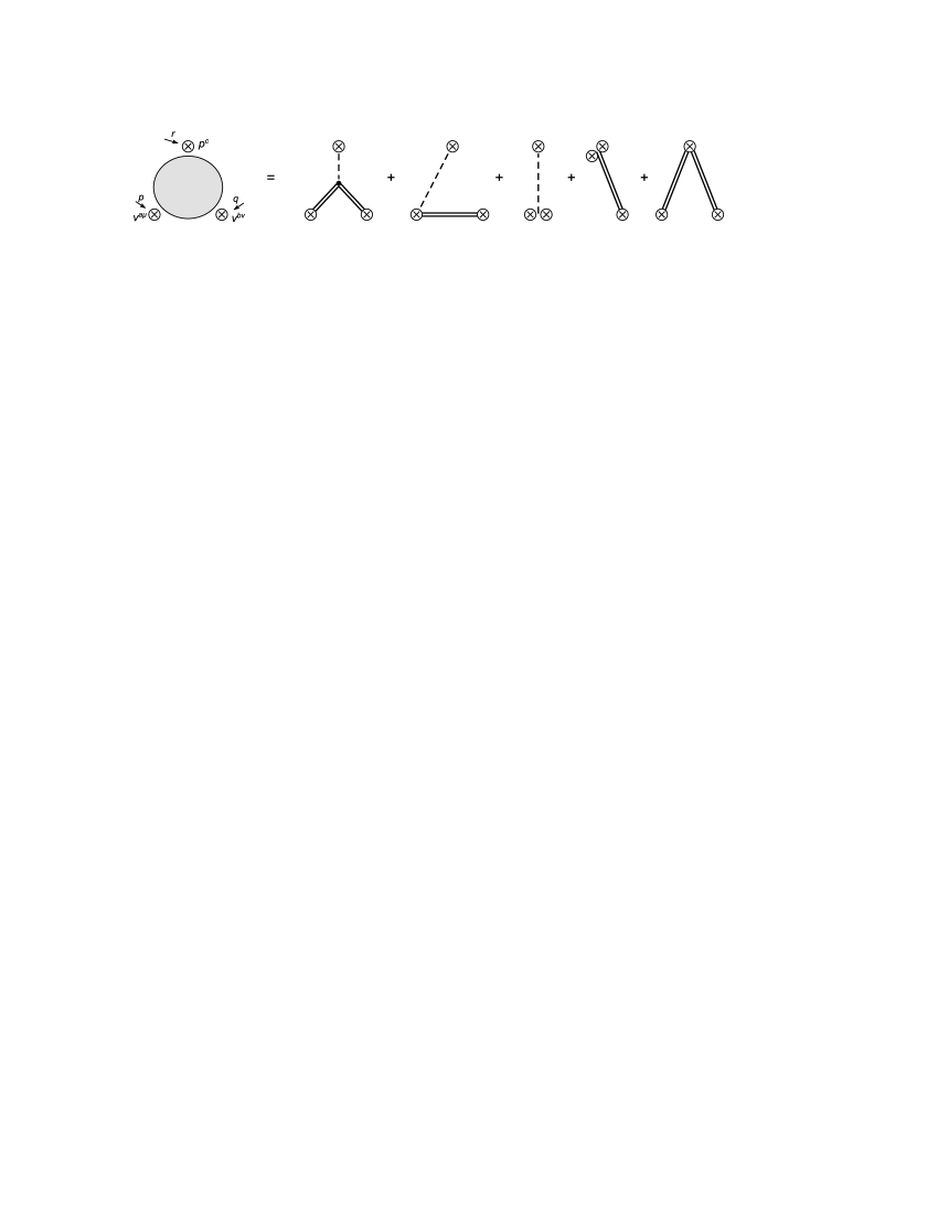
Figure 1: Diagram representation of the $VVP$ three point function in tensor field formalism. Double lines stand for vector resonances in the given formalism and dash lines for pseudoscalar mesons. Here and in the following figures, crossing is tacitly assumed.

This expression satisfies the short distance constraints (67) provided [32]

$$c_{1} = -4c_{3}\,,$$

$$c_{2} = -4c_{3}+c_{5}\,,$$

$$c_{6} = c_{5}-\frac{N_{C}}{64\sqrt{2}\pi^{2}}\frac{m}{F_{V}}\,,$$

$$d_{1} = -8d_{2}-\frac{N_{C}}{64\pi^{2}}\frac{m^{2}}{F_{V}^{2}}+\frac{F_{0}^{2}}{4F_{V}^{2}}\,,$$

$$d_{3} = -\frac{N_{C}}{64\pi^{2}}\frac{m^{2}}{F_{V}^{2}}+\frac{F_{0}^{2}}{8F_{V}^{2}}\,.$$ (70)

In this case eq. (69) simplifies to

$$\Pi_{VVP}^{T}(p^{2},q^{2},r^{2})=\frac{B_{0}F_{0}^{2}}{2}\frac{p^{2}+q^{2}+r^{2}-\frac{N_{C}}{4\pi^{2}}\frac{m^{4}}{F_{0}^{2}}}{(p^{2}-m^{2})(q^{2}-m^{2})r^{2}}\,,$$ (71)

which coincides with the lowest meson dominance (LMD) approximation developed in [7], [8].

Let us compare (69) with the analogical calculation using instead of ${\cal L}_{T}$ the strongly equivalent vector field form of the Lagrangian ${\cal L}_{V}^{\text{eff}(\leq 6)}+{\cal L}_{V}^{\text{eff}(\leq 6),contact}$. Because we have lost the complete equivalence by means of the truncation of the infinite series in (57), we expect that the result will be generally different, yielding however the same low energy expansion up to the order $O(p^{6})$. This is of course the case, the result is

$$\Pi_{VVP}^{V\text{eff}}(p^{2},q^{2},r^{2}) = \frac{B_{0}}{r^{2}}\left[-\frac{N_{C}}{8\pi^{2}}+4F_{V}^{2}\frac{(d_{1}-d_{3}+8d_{2})r^{2}+d_{3}(p^{2}+q^{2})}{m^{4}}\right.$$ (72)

$$\left.-4\sqrt{2}F_{V}\frac{(c_{1}+c_{2}-c_{5}+8c_{3})r^{2}+(c_{5}-c_{6})(p^{2}+q^{2})}{m^{3}}\right]\,.$$

It is immediately seen that $\Pi_{VVP}^{V\text{eff}}(p^{2},q^{2},r^{2})$ does not allow for the short distance constraint to be satisfied.

A natural question arises here, whether it is possible to recover the full expression (69) using some extension of the Lagrangian ${\cal L}_{V}^{\text{eff}(\leq 6)}+{\cal L}_{V}^{\text{eff}(\leq 6),\,contact}$ by means of an addition of only a finite number of terms from (57). The answer is positive for the following simple reason. Generally, the only relevant vertices which contribute to the tree graph corresponding to the $n$-point function are those satisfying $n_{S}+n_{L}\leq n$, where $n_{S}$ is  the number of the external sources $v$, $a$, $s$ or $p$ and $n_{L}$ is number of legs. Because each $J_{i}$ contains at least one of the external sources or at least one Goldstone boson leg, only finite number of terms of the Lagrangian (57) does really contribute to the $n$-point functions with $n$ fixed. In our example of three-point $VVP$ function, we can safely neglect all the contact terms composed from more than three $J_{i}$’s as well as the resonance interaction terms with one (two) resonance field and more than two (one) $J_{i}$’s. Generally, provided we require to reproduce in the vector field formalism all the three-point functions derived from ${\cal L}_{T}$, we can use e.g. the Lagrangian

$${\cal L}_{V}^{\text{eff},\,{\rm 3-point}\,}={\cal L}_{V}^{\text{eff}(6)}+{\cal L}_{V}^{\text{eff}(6),\,contact}+{\cal L}_{V}^{(8)\,{\rm 3-point}}+{\cal L}_{V}^{(10)\,\,{\rm 3-point}}$$ (73)

with additional $O(p^{8})$ and $O(p^{10})$ terms, where (cf. (59), (60))

$${\cal L}_{V}^{(8)\,{\rm 3-point}} = -\frac{1}{4}\left(\widehat{V}:\widehat{V}\right)-\frac{1}{m}\left(J_{2}^{(4)}:\widehat{V}\right)+\frac{4}{m^{3}}\left(J_{2}^{(2)}:J_{4}:\widehat{V}\right)$$ (74)

$$+\frac{2}{m^{3}}\left(J_{2}^{(2)}:J_{5}\cdot D:\widehat{V}\right)+\frac{2}{m^{3}}\left(\widehat{V}:J_{5}\cdot D:J_{2}^{(2)}\right)$$

$$-\frac{1}{m^{2}}\left(J_{2}^{(4)}:J_{2}^{(4)}\right)+\frac{8}{m^{4}}\left(J_{2}^{(2)}:J_{4}:J_{2}^{(4)}\right)$$

$$+\frac{4}{m^{4}}\left(J_{2}^{(4)}:J_{5}\cdot D:J_{2}^{(2)}\right)+\frac{4}{m^{4}}\left(J_{2}^{(2)}:J_{5}\cdot D:J_{2}^{(4)}\right)$$

and

$${\cal L}_{V}^{(10)\,\,{\rm 3-point}} = \frac{4}{m^{4}}\left(J_{2}^{(4)}:J_{4}:J_{2}^{(4)}\right)+\frac{4}{m^{3}}\left(J_{2}^{(4)}:J_{4}:\widehat{V}\right)+\frac{1}{m^{2}}\left(\widehat{V}:J_{4}:\widehat{V}\right)$$ (75)

$$+\frac{1}{m^{2}}\left(\widehat{V}:J_{5}\cdot D:\widehat{V}\right)+\frac{2}{m^{3}}\left(J_{2}^{(4)}:J_{5}\cdot D:\widehat{V}\right)$$

$$+\frac{2}{m^{3}}\left(\widehat{V}:J_{5}\cdot D:J_{2}^{(4)}\right)+\frac{4}{m^{4}}\left(J_{2}^{(4)}:J_{5}\cdot D:J_{2}^{(4)}\right)\,.$$

We have explicitly verified this statement for the $VVP$ three-point function.

For completeness, let us also briefly discuss the reversed problem, i.e. let us start with the general vector field Lagrangian ${\cal L}_{V}$ (see (6) and Appendix B) and compare the result with the strongly equivalent antisymmetric tensor field one ${\cal L}_{T}^{\text{eff},(\leq 6)}+{\cal L}_{T}^{\text{eff}(\leq 6),\,contact}$. Using ${\cal L}_{V}$, the relevant sources $J_{i}$ in the vector case are those with the couplings $h_{V}$, $f_{V}$ and $\sigma_{V}$ from Appendix B.1 and the diagrams are depicted in Fig. 2.

Figure 2: Diagram representation of the $VVP$ three point function in vector field formalism. Vector resonances are depicted now by single lines.

For the $VVP$ correlator we get the following expression [8]

$$\Pi_{VVP}^{V}(p^{2},q^{2},r^{2}) = \frac{B_{0}}{r^{2}}\left[-\frac{N_{C}}{8\pi^{2}}-4\sigma_{V}f_{V}^{2}\frac{p^{2}q^{2}}{(p^{2}-m^{2})(q^{2}-m^{2})}\right.$$ (76)

$$\left.+4\sqrt{2}h_{V}f_{V}\frac{p^{2}}{(p^{2}-m^{2})}+4\sqrt{2}h_{V}f_{V}\frac{q^{2}}{(q^{2}-m^{2})}\right]\,,$$

which, however, does not satisfy the short distance constraints (67) even if the $O(p^{6})$ contact terms of the form (65), (66) are added. On the contrary to the previous case, the Lagrangian ${\cal L}_{T}^{\text{eff},(\leq 6)}+{\cal L}_{T}^{\text{eff}(\leq 6),\,contact}$ reproduces this expression completely. The reason is, that ${\cal L}_{T}^{\text{eff},(\leq 6)}+{\cal L}_{T}^{\text{eff}(\leq 6),\,contact}$ contains already all the necessary terms (note that, ${\cal L}_{T}^{\text{eff}(2n+6)}$ with $n\geq 1$ involves only terms with at least four $J_{i}$’s and/or resonance and Goldstone boson legs and ${\cal L}_{T}^{\text{eff},(\leq 6)}+{\cal L}_{T}^{\text{eff}(\leq 6),\,contact}$ therefore already recovers all the tree level three point functions).

5 First order formalism

5.1 Motivation

As we have seen in the previous sections, neither the antisymmetric tensor nor the vector representation is “complete” in the sense that when passing to the $O(p^{6})$ effective chiral Lagrangian, some structures possible in one of them are missing in the other and vice versa. More precisely, as it was mentioned in [12] and [11], the antisymmetric tensor formalism does not create the contact term of the form (cf. (18))

$${\cal L}_{\chi}^{J_{1}}=-\frac{1}{2}\left(J_{1}\cdot J_{1}\right)\,,$$ (77)

though the term $(J_{1}.W)$ is presented in the resonance Lagrangian. In [12] for instance the following $J_{1}$ was considered in this context

$$J_{1}^{a}=-\frac{f_{\chi}}{m}\langle T^{a}[\chi_{-},u_{\mu}]\rangle$$ (78)

and the corresponding contact term ${\cal L}_{\chi}^{J_{1}}$,

$${\cal L}_{\chi}^{J_{1}}=-\frac{f_{\chi}^{2}}{2m^{2}}\langle[\chi_{-},u_{\mu}][\chi_{-},u_{\mu}]\rangle\,,$$ (79)

was added to ${\cal L}_{\chi,T}^{(6)}$ by hand. In [11], the same was done with

$$J_{1}{}_{\mu}^{a}=i\theta_{V}\varepsilon_{\mu\nu\alpha\beta}\left\langle T^{a}u^{\nu}u^{\alpha}u^{\beta}\right\rangle+h_{V}\varepsilon_{\mu\nu\alpha\beta}\left\langle T^{a}\{u^{\nu},f_{+}^{\alpha\beta}\}\right\rangle$$ (80)

and analogous source for the $1^{++}$ resonance nonet. In connection with this ad hoc procedure, a natural question arises whether there exist formulation of the resonance Lagrangian, which produces all the terms in ${\cal L}_{\chi}^{(6)}$ known form both vector and antisymmetric tensor formulations automatically. A closer look at the formula (53) suggests, that at least the term ${\cal L}_{\chi}^{J_{1}}$ together with all the terms produced by the antisymmetric tensor field Lagrangian (48) could be produced starting with the first order Lagrangian ${\cal L}_{RV}$ (derived from ${\cal L}_{T}$ by integrating in the vector field $V$)

$${\cal L}_{RV} = \frac{1}{2}m^{2}(V\cdot V)+m\left(J_{1}\cdot V\right)+\frac{1}{2}\left(J_{1}\cdot J_{1}\right)$$ (81)

$$+\frac{1}{4}m^{2}\left(R:R\right)+\left(J_{2}:R\right)+\left(R:J_{4}:R\right)$$

$$+\left(R:J_{5}\cdot D:R\right)-m\left(W\cdot V\right)\,.$$

provided we discard the contact term $\frac{1}{2}\left(J_{1}\cdot J_{1}\right)$. The role of this term, which has to be present in ${\cal L}_{RV}$, is just to cancel analogous term which could appear after the $R$ and $V$ fields have been integrated out, because the tensor formalism does not produce such a contact term and ${\cal L}_{RV}$ was constructed in order to be completely equivalent to ${\cal L}_{T}$.

5.2 Basic properties

Therefore we are encouraged to start with the following more general first order Lagrangian

$${\cal L}_{VT} = \frac{1}{4}m^{2}(R:R)+\frac{1}{2}m^{2}\left(V\cdot V\right)-\frac{1}{2}m\left(R:\widehat{V}\right)$$ (82)

$$+\left(J_{1}\cdot V\right)+\frac{1}{2}\left(V\cdot K\cdot V\right)+\left(V\cdot J_{3}:R\right)$$

$$+(R:J_{4}:R)+(R:J_{5}\cdot D:R)+\left(J_{2}:R\right)$$

$$+(R:J_{6}::RR)\,,$$

where $V$ is vector field, $\widehat{V}=\widehat{DV}$ and $R$ is antisymmetric tensor field. Note that in the notation we use, the term $-\frac{1}{2}m\left(R:\widehat{V}\right)$ is equivalent (up to total derivative) to the term $m(V\cdot W)$ with $W=D\cdot R$. The equations of motion indicate the chiral counting $R=O(p^{2})$ and $V=O(p^{3})$, we have therefore

$${\cal L}_{VT}={\cal L}_{VT}^{(4)}+{\cal L}_{VT}^{(6)}+{\cal L}_{VT}^{(8)}\,,$$ (83)

where

$${\cal L}_{VT}^{(4)} = \frac{1}{4}m^{2}(R:R)+\left(J_{2}^{(2)}:R\right)\,,$$

$${\cal L}_{VT}^{(6)} = \frac{1}{2}m^{2}\left(V\cdot V\right)-\frac{1}{2}m\left(R:\widehat{V}\right)+\left(J_{1}\cdot V\right)+\left(J_{2}^{(4)}:R\right)$$

$$+\left(V\cdot J_{3}:R\right)+(R:J_{4}:R)+(R:J_{5}\cdot D:R)+(R:J_{6}::RR)\,,$$

$${\cal L}_{VT}^{(8)} = \frac{1}{2}\left(V\cdot K\cdot V\right)\,.$$

Solutions of the equations of motion to the lowest order read

$$R^{(2)} = -\frac{2}{m^{2}}J_{2}^{(2)}\,,$$

$$V^{(3)} = -\frac{1}{m^{2}}\left(J_{1}-\frac{2}{m^{2}}J_{3}:J_{2}^{(2)}-\frac{2}{m}D\cdot J_{2}^{(2)}\right)\,.$$

Inserting this to the original Lagrangian we obtain the effective chiral Lagrangian up to the order $O(p^{6})$ in the form

$${\cal L}_{\chi,VT}={\cal L}_{\chi,VT}^{(4)}+{\cal L}_{\chi,VT}^{(6)}\,,$$ (84)

where

$${\cal L}_{\chi,VT}^{(4)} = -\frac{1}{m^{2}}\left(J_{2}^{(2)}:J_{2}^{(2)}\right)\,,$$

$${\cal L}_{\chi,VT}^{(6)} = -\frac{1}{2m^{2}}\left(J_{1}\cdot J_{1}\right)-\frac{2}{m^{2}}\left(J_{2}^{(2)}:J_{2}^{(4)}\right)-\frac{8}{m^{6}}(J_{2}^{(2)}:J_{6}::J_{2}^{(2)}J_{2}^{(2)})$$

$$+\frac{2}{m^{3}}\left(D\cdot J_{2}^{(2)}\cdot J_{1}\right)+\frac{2}{m^{4}}\left(D\cdot J_{2}^{(2)}\cdot J_{2}^{(2)}\cdot\overleftarrow{D}\right)$$

$$-\frac{4}{m^{5}}(D\cdot J_{2}^{(2)}\cdot J_{3}:J_{2}^{(2)})+\frac{4}{m^{4}}(J_{2}^{(2)}:J_{4}:J_{2}^{(2)})+\frac{4}{m^{4}}(J_{2}^{(2)}:J_{5}\cdot D:J_{2}^{(2)})$$

$$-\frac{2}{m^{6}}(J_{2}^{(2)}:J_{3}\cdot J_{3}:J_{2}^{(2)})+\frac{2}{m^{4}}(J_{1}\cdot J_{3}:J_{2}^{(2)})\,.$$

Note that we have reproduced with the Lagrangian ${\cal L}_{VT}$ all the terms, which yield the vector and tensor representation, and two new terms in the last line. As an example of (84) we have calculated in Appendix C the resonance saturation of some of the $O(p^{6})$ LECs of the canonical basis [37] by means of ${\cal L}_{VT}$ with sources listed in Appendix B.3. This can be compared with tensor formalism given in [12].

Note also that ${\cal L}_{\chi,VT}^{(6)}$ can be rewritten in the more condensed form

$${\cal L}_{\chi,VT}^{(6)}=-\frac{1}{2m^{2}}\left(\widetilde{J}_{1}\cdot\widetilde{J}_{1}\right)-\frac{2}{m^{2}}\left(J_{2}^{(2)}:\widetilde{J}_{2}^{(4)}\right)+\frac{4}{m^{4}}(J_{2}^{(2)}:J_{5}\cdot D:J_{2}^{(2)})\,,$$ (85)

where

$$\widetilde{J}_{1} = J_{1}-\frac{2}{m}J_{2}^{(2)}:J_{3}-\frac{2}{m}D\cdot J_{2}^{(2)}\,,$$

$$\widetilde{J}_{2}^{(4)} = J_{2}^{(4)}-\frac{2}{m^{2}}J_{4}:J_{2}^{(2)}+\frac{4}{m^{4}}J_{6}::J_{2}^{(2)}J_{2}^{(2)}\,.$$

This indicates some redundancy of the Lagrangian (82), as far as the $O(p^{6})$ effective chiral Lagrangian is concerned. This redundancy reflects the possibility of field redefinitions according to the prescription

$$R \rightarrow R-\frac{2}{m^{2}}\delta J_{4}:R-\frac{2}{m^{2}}V\cdot\delta^{(1)}J_{3}-\frac{2}{m^{2}}\delta J_{6}::RR\,,$$

$$V \rightarrow V-\frac{1}{m^{2}}\delta^{(2)}J_{3}:R\,,$$ (86)

which reproduces (up to the terms of the chiral order $O(p^{8})$) the form of the Lagrangian ${\cal L}_{VT}$ with the shifts of the sources

$$J_{1} \rightarrow J_{1}-\frac{2}{m^{2}}\delta^{(1)}J_{3}:J_{2}^{(2)}\,,$$

$$J_{2}^{(4)} \rightarrow J_{2}^{(4)}-\frac{2}{m}\delta J_{4}:J_{2}^{(2)}-\frac{1}{m^{2}}J_{1}\cdot\delta^{(2)}J_{3}\,,$$

$$J_{3} \rightarrow J_{3}-\delta^{(1)}J_{3}-\delta^{(2)}J_{3}\,,$$

$$J_{4} \rightarrow J_{4}-\delta J_{4}-\frac{2}{m^{2}}J_{2}^{(2)}:\delta J_{6}\,,$$

$$J_{5} \rightarrow J_{5}-\frac{1}{2}\widehat{g\delta^{(2)}J}_{3}\,,$$

$$J_{6} \rightarrow J_{6}-\delta J_{6}\,.$$ (87)

5.3 Correspondence with vector and antisymmetric tensor formalism

Let us now establish the equivalence of this formalism with usual vector and tensor representation. Writing

$$Z_{VT}[J_{i},K]=\int{\cal D}R{\cal D}V\exp\left(i\int d^{4}x{\cal L}_{VT}\right)\,,$$ (88)

we can integrate out either the vector field or the antisymmetric tensor field and get

$$Z_{VT}[J_{i},K]=\int{\cal D}R\exp\left(i\int d^{4}x{\cal L}_{T}^{\text{eff}}\right)=\int{\cal D}V\exp\left(i\int d^{4}x{\cal L}_{V}^{\text{eff}}\right)\,.$$ (89)

Using the formulae given in the preceding sections we end up with

$${\cal L}_{T}^{\text{eff}} = \frac{1}{4}m^{2}\left(R:R\right)+\left(J_{2}:R\right)+(R:J_{4}:R)+(R:J_{5}\cdot D:R)$$ (90)

$$-\frac{1}{2m^{2}}(J_{1}+R:J_{3}+mW)^{2}+(R:J_{6}::RR)$$

$$-\frac{1}{2m^{2}}\sum_{n=1}^{\infty}\left(-\frac{1}{m^{2}}\right)^{n}\left(J_{1}+R:J_{3}+mW\right)\cdot K^{n}\cdot\left(J_{1}+R:J_{3}+mW\right)\,,$$

i.e., up to $O(p^{6})$

$${\cal L}_{T}^{\text{eff}}= -\frac{1}{2}\left(W\cdot W\right)+\frac{1}{4}m^{2}\left(R:R\right)$$

$$+\left(J_{1}^{\text{eff}}\cdot W\right)+\left(J_{2}^{\text{eff}}:R\right)+\left(W\cdot J_{3}^{\text{eff}}:R\right)+\left(R:J_{4}^{\text{eff}}:R\right)+\left(R:J_{5}^{\text{eff}}\cdot D:R\right)$$

$$+(R:J_{6}^{\text{eff}}::RR)+{\cal L}_{T}^{\text{eff},contact}$$ (91)

with

$${\cal L}_{T}^{\text{eff},contact}=-\frac{1}{2m^{2}}(J_{1}\cdot J_{1})$$

and

$$J_{1}^{\text{eff}} =-\frac{1}{m}J_{1}\,, J_{2}^{\text{eff}} =J_{2}-\frac{1}{m^{2}}J_{1}\cdot J_{3}\,,$$

$$J_{3}^{\text{eff}} =-\frac{1}{m}J_{3}\,, J_{4}^{\text{eff}} =J_{4}-\frac{1}{2m^{2}}J_{3}\cdot J_{3}\,,$$

$$J_{5}^{\text{eff}} =J_{5}\,, J_{6}^{\text{eff}} =J_{6}\,.$$

As in the tensor case, the cubic term can be put off – according to (87) we can effectively absorbed the source $J_{6}$ in $J_{4}$. We thus get

$${\cal L}_{V}^{\text{eff}} = \frac{1}{2}m^{2}\left(V\cdot V\right)+\left(J_{1}\cdot V\right)+\frac{1}{2}\left(V\cdot K\cdot V\right)$$

$$-\frac{1}{m^{2}}(J_{2}-\frac{1}{2}m\widehat{V}+V\cdot J_{3}):(J_{2}-\frac{1}{2}m\widehat{V}+J_{3}\cdot V)-\frac{1}{m^{2}}\sum_{n=1}^{\infty}\left(-\frac{4}{m^{2}}\right)^{n}$$

$$\times(J_{2}-\frac{1}{2}m\widehat{V}+V\cdot J_{3}):(J_{4}-\frac{2}{m^{2}}J_{2}^{(2)}:J_{6}+J_{5}\cdot D)^{n}:(J_{2}-\frac{1}{2}m\widehat{V}+J_{3}\cdot V)\,,$$

i.e. up to $O(p^{6})$

$${\cal L}_{V}^{\text{eff}}=-\frac{1}{4}\left(\widehat{V}:\widehat{V}\right)+\frac{1}{2}m^{2}(V\cdot V)+(J_{1}^{\text{eff}}\cdot V)+\left(J_{2}^{\text{eff}}:\widehat{V}\right)+{\cal L}_{V}^{\text{eff},contact}$$ (93)

with

$${\cal L}_{V}^{\text{eff},contact} = -\frac{1}{m^{2}}\left(J_{2}^{(2)}:J_{2}^{(2)}\right)-\frac{2}{m^{2}}\left(J_{2}^{(4)}:J_{2}^{(2)}\right)$$

$$+\frac{4}{m^{4}}(J_{2}^{(2)}:J_{4}:J_{2}^{(2)})+\frac{4}{m^{4}}(J_{2}^{(2)}:J_{5}\cdot D:J_{2}^{(2)})-\frac{8}{m^{6}}(J_{2}^{(2)}:J_{6}::J_{2}^{(2)}J_{2}^{(2)})$$

and

$$J_{1}^{\text{eff}} =J_{1}-\frac{2}{m^{2}}J_{2}^{(2)}:J_{3}\,, J_{2}^{\text{eff}} =\frac{1}{m}J_{2}^{(2)}\,.$$

5.4 $VVP$ correlator

Let us now return to the explicit example of the $VVP$ correlator. Within the first order formalism we should take more general $J_{i}$ than in the vector and tensor case. The reason is, that the integration by parts reducing the number of independent terms re-distributing them between $J_{1}$ and $J_{2}$ and between $J_{3}$ and $J_{4,5}$ (cf. (14)) is not possible here. More detailed discussion as well as the explicit form of the sources is given in Appendix B.3.

Using the Feynman rules described in the Appendix A and performing the evaluation of the graphs depicted in Fig. 3 we get

$$\Pi_{VVP}^{VT}(p^{2},q^{2},r^{2})=B_{0}\Bigl{[}-\frac{N_{C}}{16\pi^{2}r^{2}}+\frac{4\sqrt{2}h_{V}p^{2}}{(p^{2}-m^{2})r^{2}}\left(f_{V}-\frac{F_{V}}{m}\right)$$

$$\quad+2\left(F_{V}-f_{V}\frac{p^{2}}{m}\right)\left(F_{V}-f_{V}\frac{q^{2}}{m}\right)\frac{(d_{1}+8d_{2}-d_{3})r^{2}+2d_{3}p^{2}}{(p^{2}-m^{2})(q^{2}-m^{2})r^{2}}$$

$$\quad+\frac{2\sqrt{2}}{m}\left(F_{V}-f_{V}\frac{p^{2}}{m}\right)\frac{(c_{1}+c_{2}+8c_{3}-c_{5})r^{2}+(-c_{1}+c_{2}+c_{5}-2c_{6})p^{2}+(c_{1}-c_{2}+c_{5})q^{2}}{(p^{2}-m^{2})r^{2}}$$

$$\quad+\frac{2\sigma_{V}m}{(p^{2}-m^{2})(q^{2}-m^{2})r^{2}}\left(f_{V}-\frac{F_{V}}{m}\right)\left(F_{V}-f_{V}\frac{q^{2}}{m}\right)p^{2}+(p\leftrightarrow q)\Bigr{]}.$$ (94)

Note that for $f_{V}=h_{V}=\sigma_{V}=0$ we reproduce $\Pi_{VVP}^{T}(p^{2},q^{2},r^{2})$ (see eq. (69)) , while for $F_{V}=c_{i}=d_{i}=0$ we recover $\Pi_{VVP}^{V}(p^{2},q^{2},r^{2})$ (see eq. (76)).

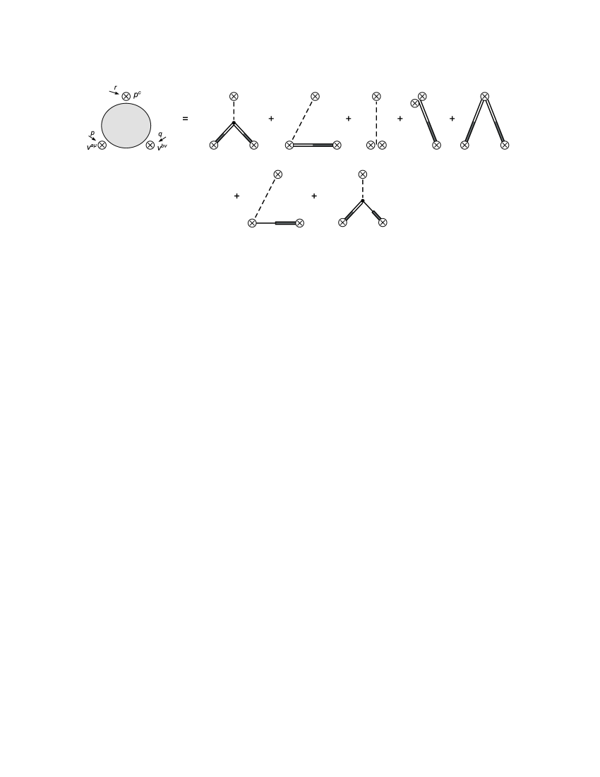
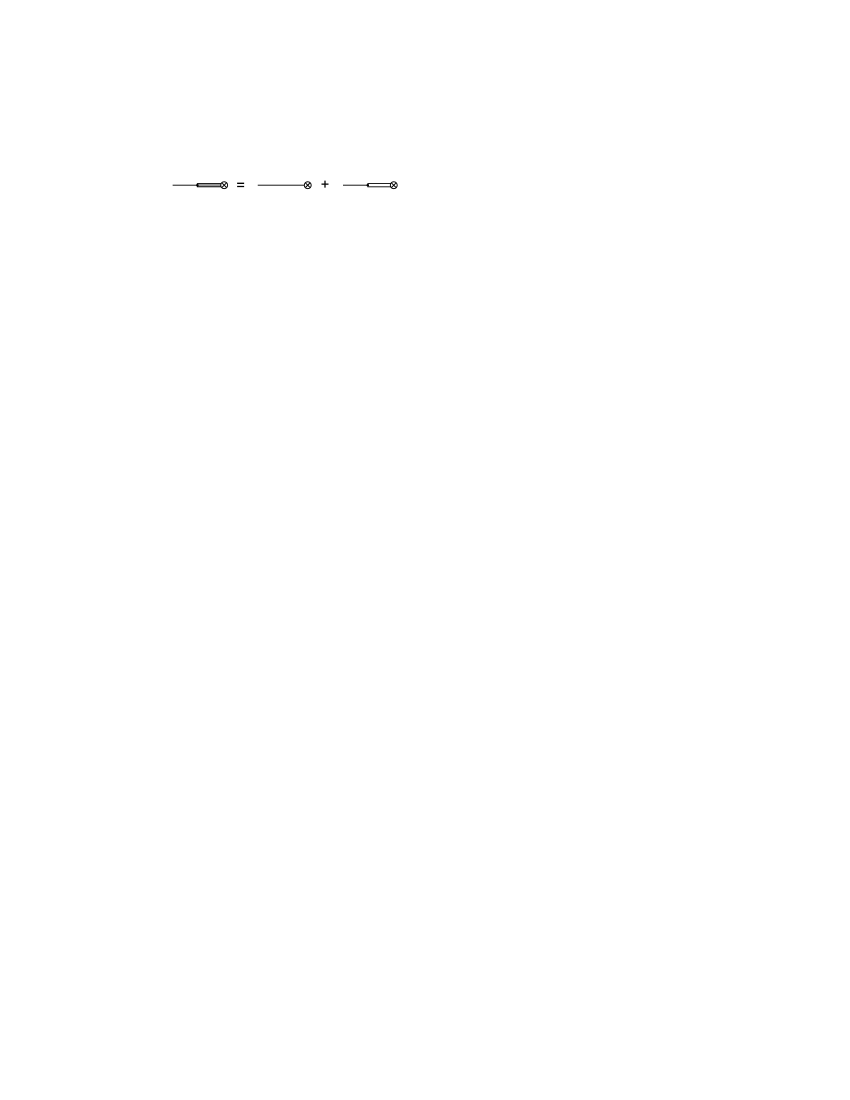
Figure 3: Diagram representation of $VVP$ three point function in the first order formalism. For limiting the number of graphs we have represented a pair of resonance propagators by shaded double line as   and   .

The $VVP$ three point function $\Pi_{VVP}^{VT}(p^{2},q^{2},r^{2})$ does not satisfy the short distance constraint unless $f_{V}=0$ and the following relations for the couplings hold

$$c_{1} = -4c_{3}\,,$$

$$c_{2} = -4c_{3}+c_{5}\,,$$

$$c_{6} = c_{5}-\frac{N_{C}}{64\sqrt{2}\pi^{2}}\frac{m}{F_{V}}\,,$$

$$d_{1} = -8d_{2}+\frac{\sigma_{V}}{2m}-\frac{N_{C}}{64\pi^{2}}\frac{m^{2}}{F_{V}^{2}}+\frac{F_{0}^{2}}{4F_{V}^{2}}\,,$$

$$d_{3} = \frac{\sigma_{V}}{2m}-\frac{N_{C}}{64\pi^{2}}\frac{m^{2}}{F_{V}^{2}}+\frac{F_{0}^{2}}{8F_{V}^{2}}\,.$$

Again the LMD approximation (71) is reproduced in this case.

6 Summary

In this paper we have studied the formal relationship of the Proca field and antisymmetric tensor field formalisms for describing massive spin-1 particles in the general context of chiral resonance Lagrangians. We have concentrated on the various levels of equivalence of the corresponding Lagrangians (6), (11) and tried to partially enlarge the $O(p^{4})$ analysis of ref. [21] to the order $O(p^{6})$.

In this case, the situation is more involved, because at this order the chiral resonance Lagrangian generally contain new types of bi(tri)linear couplings of the resonance fields to the chiral building blocks. As a result, contrary to the $O(p^{4})$ case, the complete equivalence (on the resonance level) of a local $O(p^{6})$ Lagrangian within one formalism cannot be generally achieved by means of a complementary finite chiral order Lagrangian which is local and has finite number of interaction and contact terms. Using the path integral method, previously used in this context in [29] and [30], we have established the nonlocal Lagrangians ${\cal L}_{T}^{\text{eff}}$ and ${\cal L}_{V}^{\text{eff}}$ (cf. (44), (57)) completely equivalent to ${\cal L}_{V}$ and ${\cal L}_{T}$ respectively.

On the other hand, provided we restrict ourselves to the $n-$point correlators with $n\leq n_{\max}$, we can always reproduce them completely with the complementary Lagrangian with finite number of terms and finite chiral order $n_{\chi}\geq 6$. We have explicitly illustrated this using the $VVP$ three point correlator as an explicit example.

Expanding the nonlocality of ${\cal L}_{T}^{\text{eff}}$ and ${\cal L}_{V}^{\text{eff}}$ and keeping terms up to the chiral order $O(p^{6})$ we have obtained local Lagrangians ${\cal L}_{T}^{\text{eff},\,(\leq 6)}+{\cal L}_{T}^{\text{eff},\,(\leq 6)contact}$ and ${\cal L}_{V}^{\text{eff},\,(\leq 6)}+{\cal L}_{V}^{\text{eff},\,(\leq 6)contact}$ strongly equivalent to ${\cal L}_{V}$ and ${\cal L}_{T}$ respectively (i.e. producing the same effective chiral Lagrangian up to $O(p^{6})$).

There is also another aspect of the $O(p^{6})$ chiral resonance Lagrangians we have addressed. While at the order $O(p^{4})$, the antisymmetric tensor formalism is more complete in the sense that it produces all the possible structures in the effective $O(p^{4})$ chiral Lagrangian, at the order $O(p^{6})$ neither the vector nor the antisymmetric tensor formalism has this property. We have therefore suggested an alternative first order formalism, in the framework of which the spin-1 particles are described in terms of a pair of vector and antisymmetric tensor fields. Within this formalism, all the structures of the effective chiral Lagrangian which are known from the vector and antisymmetric tensor representations are reproduced all at once with certain additional terms. As we have shown in the special case of the $VVP$ correlator, provided we take the most general chiral building block to which the vector and antisymmetric tensor fields can couple, we recover all the contributions coming from the Lagrangians ${\cal L}_{V}$ and ${\cal L}_{T}$ at the resonance level. This formalism also in some sense legitimizes the ad hoc addition of the missing contact terms to the antisymmetric tensor formalism in order to make the $O(p^{6})$ effective chiral Lagrangian complete. Of course the final decision justifying presence of such terms in ${\cal L}_{T}$ should by dictated by asymptotic high energy constraints (cf. [21, 11]).

We have also studied the relationship of this first order representation to the previous two. Again the completely equivalent Lagrangians ${\cal L}_{T}^{\text{eff}}$ and ${\cal L}_{V}^{\text{eff}}$ are generally nonlocal and strongly equivalent local Lagrangians ${\cal L}_{T}^{\text{eff},\,(\leq 6)}+{\cal L}_{T}^{\text{eff},\,(\leq 6)contact}$ and ${\cal L}_{V}^{\text{eff},\,(\leq 6)}+{\cal L}_{V}^{\text{eff},\,(\leq 6)contact}$ can be constructed keeping terms up to the order $O(p^{6})$ only.

We have also briefly touched the issue of the short distance constraints restricting the possible form of the chiral building blocks which appear in the chiral resonance Lagrangian. For the $VVP$ correlator, which we have studied in detail, it has been known [32], that the antisymmetric tensor representation was compatible with the requirements dictated by the leading order OPE, while the usual vector field representation was not [8]. However, the known correspondence of the vector and antisymmetric representation can be applied here in order to construct vector field chiral resonance Lagrangian, which for this special correlator reproduces exactly the result of the antisymmetric tensor formalism and therefore yield the result compatible with OPE. The price to pay is the necessity to introduce terms up to the chiral order $O(p^{10})$.

As far as the first order formalism is concerned, because it is a synthesis of the previous two, it can be therefore easily made compatible with the short distance constraints for the $VVP$ correlator.

Appendix A Formal properties of the first order formalism

In this Appendix we summarize the properties of the first order formalism introduced in Section 5. Let us consider the simplified case with only one pair of (real) fields and the Lagrangian with two external sources $J_{1,2}$

$${\cal L}_{VT} = \frac{1}{4}m^{2}R:R+\frac{1}{2}m^{2}V\cdot V-\frac{1}{2}mR:\widehat{V}$$ (95)

$$+\left(J_{1}\cdot V\right)+\left(J_{2}:R\right)\,,$$

where $\widehat{V}=\widehat{\partial V}$. The equation of motion are then

$$\frac{1}{2}m^{2}R-\frac{1}{2}m\widehat{V} = -J_{2}\,,$$

$$m^{2}V+mW = -J_{1}\,,$$ (96)

where $W=\partial\cdot R$. From the first equation it follows

$$\partial\cdot\widehat{V}-mW=\frac{2}{m}\partial\cdot J_{2}$$ (97)

and, when combined with the second one we get Proca equation for the $V$ field

$$\partial\cdot\widehat{V}+m^{2}V=\frac{2}{m}\partial\cdot J_{2}-J_{1}\,.$$ (98)

From the second eq. (96) we get

$$\widehat{\partial W}+m\widehat{V}=-\frac{1}{m}\widehat{\partial J_{1}}\,.$$ (99)

This can be combined with the first eq. (96) to obtain the standard equation for the antisymmetric tensor field.

$$\widehat{\partial W}+m^{2}R=-\frac{1}{m}\widehat{\partial J_{1}}-2J_{2}\,.$$ (100)

We have therefore in the momentum representation (in our notation $\widetilde{A}(p)=\int d^{4}x{\rm{e}}^{{\rm{i}}p\cdot x}A(x)$)

$$\widetilde{V}(p) = -\Delta_{F}^{V}(p)\cdot\left(\widetilde{J}_{1}(p)+\frac{2{\rm i}}{m}p\cdot\widetilde{J}_{2}(p)\right)\,,$$

$$\widetilde{R}(p) = -\Delta_{F}^{R}(p):\left(\widetilde{J}_{2}(p)-\frac{{\rm i}}{2m}\widehat{p\widetilde{J}_{1}(p)}\right)$$ (101)

and thus

$$\left(\begin{array}[]{l}\widetilde{V}(p)\\ \widetilde{R}(p)\end{array}\right)=-\left(\begin{array}[]{ll}\Delta_{F}^{V}(p)&-\frac{{\rm i}}{m}\widehat{\Delta_{F}^{V}(p)p}\\ \frac{{\rm i}}{m}\Delta_{F}^{R}(p)\cdot p&\Delta_{F}^{R}(p)\end{array}\right)\left(\begin{array}[]{l}\widetilde{J}_{1}(p)\\ \widetilde{J}_{2}(p)\end{array}\right)\,,$$ (102)

where

$${\rm i}\Delta_{F}^{V}(p)_{\mu\nu} = -\frac{{\rm i}}{p^{2}-m^{2}+{\rm i}0}\left(g_{\mu\nu}-\frac{p_{\mu}p_{\nu}}{m^{2}}\right)\,,$$

$${\rm i}\Delta_{F}^{R}(p)_{\mu\nu\,\,\rho\sigma} = -\frac{{\rm i}}{p^{2}-m^{2}+{\rm i}0}\frac{1}{m^{2}}\left((m^{2}-p^{2})g_{\mu\rho}g_{\nu\sigma}+g_{\mu\rho}p_{\nu}p_{\sigma}-g_{\mu\sigma}p_{\nu}p_{\rho}-(\mu\leftrightarrow\nu)\right)\,.$$

It is not difficult to prove, that

$$\Delta_{F}^{RV}(p)=-\frac{{\rm i}}{m}\widehat{\Delta_{F}^{V}(p)p}=-\frac{{\rm i}}{m}\Delta_{F}^{R}(p)\cdot p\,.$$ (103)

The matrix of the momentum space propagators is therefore

$$\Delta_{F}(p)=\left(\begin{array}[]{ll}\Delta_{F}^{V}(p)&\Delta_{F}^{RV}(p)\\ \Delta_{F}^{RV}(-p)^{T}&\Delta_{F}^{R}(p)\end{array}\right)$$ (104)

and the off-diagonal propagator is

$$i\Delta_{F}^{RV}(p)_{\sigma,\mu\nu}=\frac{{\rm i}}{p^{2}-m^{2}+{\rm i}0}\frac{{\rm i}}{m}(g_{\sigma\mu}p_{\nu}-g_{\sigma\nu}p_{\mu})\,.$$ (105)

The two-point functions are then

$$=\langle T\widetilde{V}_{\mu}(p)V_{\nu}(0)\rangle ={\rm i}\Delta_{F}^{V}(p)_{\mu\nu}\,,$$

$$=\langle T\widetilde{R}_{\mu\nu}(p)R_{\rho\sigma}(0)\rangle ={\rm i}\Delta_{F}^{R}(p)_{\mu\nu\,\,\rho\sigma}\,,$$

$$=\langle T\widetilde{V}_{\sigma}(p)R_{\mu\nu}(0)\rangle ={\rm i}\Delta_{F}^{RV}(p)_{\sigma\,\,\mu\nu}\,,$$

$$=\langle T\widetilde{R}_{\mu\nu}(p)V_{\sigma}(0)\rangle ={\rm i}\Delta_{F}^{RV}(-p)_{\sigma\,\,\mu\nu}=-{\rm i}\Delta_{F}^{RV}(p)_{\sigma\,\,\mu\nu}$$ (106)

and the wave functions to be attached to the on-shell external lines are

$$\langle 0|V_{\mu}(0)|k\rangle = \varepsilon_{\mu}(k)\,,$$

$$\langle 0|R_{\mu\nu}(0)|k\rangle = -\frac{{\rm i}}{m}\left(k_{\mu}\varepsilon_{\nu}(k)-k_{\nu}\varepsilon_{\mu}(k)\right)\,.$$ (107)

Appendix B Structure of the $J_{i}$’s

In this appendix we summarize explicit structure of sources $J_{i}$ needed in the main text expressed by means of chiral building blocks. Our aim is not to give an exhausting list of all $J_{i}$, instead we collect existing terms from the literature. We preserve notation for couplings already developed there. In the case of the first order formalism we combine both couplings from the vector and tensor Lagrangians. Of course also in this case we do not attempt to give a complete list.

In the following formulae, $T^{a}=\lambda^{a}/\sqrt{2}$, where $\lambda^{a}$ are the Gell-Mann matrices and (in the next subsections) $\lambda^{0}=\sqrt{\frac{2}{3}}\,\mathbf{1}$. The standard chiral building blocks are (for details see e.g. [37]).

$$u = \exp\left({\rm i}\phi^{a}T^{a}/\sqrt{2}\right)\,,$$

$$u_{\mu} = i[u^{\dagger}(\partial_{\mu}-ir_{\mu})u-u(\partial_{\mu}-il_{\mu})u^{\dagger}]\,,$$

$$D_{\mu} = \partial_{\mu}+\Gamma_{\mu}\,,$$

$$\Gamma_{\mu} = \frac{1}{2}[u^{\dagger}(\partial_{\mu}-ir_{\mu})u+u(\partial_{\mu}-il_{\mu})u^{\dagger}]\,,$$

$$f_{\pm\mu\nu} = uf_{L\,\mu\nu}u^{\dagger}\pm u^{\dagger}f_{R\,\mu\nu}u\,,$$

$$\chi_{\pm} = u^{\dagger}\chi u^{\dagger}\pm u\chi^{\dagger}u\,,$$

$$h_{\mu\nu} = D_{\mu}u_{\nu}+D_{\nu}u_{\mu}\,.$$ (108)

B.1 Vector field formalism

The $J_{i}$ corresponding to the vector field formulation (6) we take from [31] (see also [8])

Parity even sector

• $J_{1}$

  Term $$J_{1}{}_{\mu}^{a}$$ coupling

  1

  2

• $J_{2}$

  Term $$J_{2}{}_{\mu\nu}^{a}$$ coupling

  1

  2

• $K$

  Term $$K_{\mu\nu}^{ab}$$ coupling

  1

  2

  3

  4

  5

  6

  7

Parity odd sector

• $J_{1}$

  Term $$J_{1}{}_{\mu}^{a}$$ coupling

  1

  2

• $J_{3}$

  Term $$J_{3}{}_{\mu\nu}^{ab\alpha}$$ coupling

  1

B.2 Antisymmetric tensor field formalism

Parity even sector to $O(p^{4})$ (cf. [10] )

• $J_{2}^{(2)}$

  Term $$J_{2}{}_{\mu\nu}^{a}$$ coupling

  1

  2

Parity even sector $O(p^{6})$ (here we give only the symmetry breaking terms discussed in [12]; the complete list including also $J_{6}$ can be found in [11])

• $J_{1}$

  Term $$J_{1}{}_{\mu}^{a}$$ coupling

  1

• $J_{2}^{(4)}$

  Term $$J_{2}{}_{\mu\nu}^{a}$$ coupling

  1 i

  2 i

  3

  4

• $J_{4}$

  Term $$J_{4}{}_{\mu\nu\,\,\alpha\beta}^{ab}$$ coupling

  1

Parity odd sector to $O(p^{6})$ (here we list the terms given in [32], which are relevant for the calculation of the $VVP$ correlator; cf. also [22])

• $J_{2}^{(4)}$

  Term $$J_{2}{}_{\mu\nu}^{a}$$ coupling

  1

  2

  3

  4 i

  5

  6

  7

• $J_{4}$

  Term $$J_{4}{}_{\mu\nu\,\,\alpha\beta}^{ab}$$ coupling

  1

  2

• $J_{5}$

  Term $$J_{5\,\mu\nu\,\,\rho\sigma}^{ab\,\alpha}$$ coupling

  1

  2

B.3 First order formalism

For the first order formalism we can take $J_{2}^{(2)}$, $J_{4}$, $J_{5}$ and $J_{6}$ from the tensor formalism (see previous subsection). As far as $K$ and $J_{3}$ are concerned we take them from the vector case, but in order to preserve the dimension of the coupling $\sigma_{V}$, we have included one extra power of the mass $m$ in the definition of $J_{3}$ (see below). The source $J_{1}$ incorporates all the structure from the vector case supplemented with two additional terms inferred from vector $J_{2}$ by means of integration by parts. Similarly for parity even $J_{2}^{(4)}$, which we take from the tensor case while parity odd $J_{2}^{(4)}$ stay unchanged. Though we preserve the notation from the vector and tensor case, the phenomenological meaning of the couplings can be different. Here we list only the differences:

Parity even $O(p^{6})$

• $J_{1}$

  Term $$J_{1}{}_{\mu}^{a}$$ coupling

  1

  2

  3

  4

• $J_{2}^{(4)}$

  Term $$J_{2}{}_{\mu\nu}^{a}$$ coupling

  1 i

  2 i

  3

  4

  5

Parity odd $O(p^{6})$

• $J_{1}$

  Term $$J_{1}{}_{\mu}^{a}$$ coupling

  1

  2

• $J_{3}$

  Term $$J_{3}{}_{\mu\nu}^{ab\alpha}$$ coupling

  1

Appendix C Resonance contributions to the LECs

This appendix summarizes saturation of the LECs of the canonical basis given in [37] of the three flavour case ($n=3$ in the following table)

$${\cal L}_{6}=\sum_{i=1}^{94}C_{i}O_{i}\,,$$ (109)

induced by the first order resonance Lagrangian ${\cal L}_{\chi,VT}^{(6)}$ of (84). The sources we have used are only those which are summarized in the preceding appendix and are needed for constructions of chiral symmetry breaking terms. Thus the saturation of LECs summarized in the next table is not complete and can be compared with the similar results given in eqs.(62) of [12].

$i$	$C_{i}^{R}$	$i$	$C_{i}^{R}$
1	$\frac{G_{V}^{2}}{8m^{4}}+\frac{g_{V}^{2}}{8m^{2}}-\frac{G_{V}g_{V}}{4m^{3}}$	4	$\frac{G_{V}^{2}}{8m^{4}}+\frac{g_{V}^{2}}{8m^{2}}-\frac{G_{V}g_{V}}{4m^{3}}$
5	$-\frac{G_{V}g_{V2}^{m}}{\sqrt{2}m^{3}}$	8	$\frac{{e_{V}^{m}}G_{V}^{2}}{2m^{4}}-\frac{\sqrt{2}G_{V}g_{V1}^{m}}{m^{3}}$
10	$-\frac{{e_{V}^{m}}G_{V}^{2}}{2m^{4}}+\frac{\sqrt{2}G_{V}g_{V1}^{m}}{m^{3}}+\frac{G_{V}g_{V2}^{m}}{\sqrt{2}m^{3}}$	22	$\frac{G_{V}^{2}}{16m^{4}}+\frac{G_{V}f_{\chi}}{2\sqrt{2}m^{3}}+\frac{g_{V}\beta_{V}}{2\sqrt{2}m^{2}}+\frac{g_{V}^{2}}{16m^{2}}-\frac{G_{V}\beta_{V}}{2\sqrt{2}m^{3}}-\frac{G_{V}g_{V}}{8m^{3}}$
24	$\frac{G_{V}^{2}}{4nm^{4}}+\frac{g_{V}^{2}}{4nm^{2}}-\frac{G_{V}g_{V}}{2nm^{3}}$	25	$-\frac{3G_{V}^{2}}{8m^{4}}-\frac{G_{V}f_{\chi}}{\sqrt{2}m^{3}}-\frac{g_{V}\beta_{V}}{\sqrt{2}m^{2}}-\frac{3g_{V}^{2}}{8m^{2}}+\frac{G_{V}\beta_{V}}{\sqrt{2}m^{3}}+\frac{3G_{V}g_{V}}{4m^{3}}$
26	$(1-\frac{2}{n^{2}})\frac{G_{V}^{2}}{4m^{4}}+\frac{G_{V}f_{\chi}}{\sqrt{2}m^{3}}+\frac{\beta_{V}^{2}}{m^{2}}+\frac{g_{V}\beta_{V}}{\sqrt{2}m^{2}}+(1-\frac{2}{n^{2}})\frac{g_{V}^{2}}{4m^{2}}-\frac{G_{V}\beta_{V}}{\sqrt{2}m^{3}}-(1-\frac{2}{n^{2}})\frac{G_{V}g_{V}}{2m^{3}}$	27	$-(\frac{1}{n}-\frac{2}{n^{2}})\frac{G_{V}^{2}}{4m^{4}}-(\frac{1}{n}-\frac{2}{n^{2}})\frac{g_{V}^{2}}{4m^{2}}+(\frac{1}{n}-\frac{2}{n^{2}})\frac{G_{V}g_{V}}{2m^{3}}$
28	$\frac{G_{V}^{2}}{8n^{2}m^{4}}+\frac{g_{V}^{2}}{8n^{2}m^{2}}-\frac{G_{V}g_{V}}{4n^{2}m^{3}}$	29	$-(1+\frac{2}{n^{2}})\frac{G_{V}^{2}}{8m^{4}}-\frac{G_{V}f_{\chi}}{\sqrt{2}m^{3}}-\frac{\beta_{V}^{2}}{m^{2}}-\frac{g_{V}\beta_{V}}{\sqrt{2}m^{2}}-(1+\frac{2}{n^{2}})\frac{g_{V}^{2}}{8m^{2}}+\frac{G_{V}\beta_{V}}{\sqrt{2}m^{3}}+(1+\frac{2}{n^{2}})\frac{G_{V}g_{V}}{4m^{3}}$
30	$\frac{G_{V}^{2}}{4n^{2}m^{4}}+\frac{g_{V}^{2}}{4n^{2}m^{2}}-\frac{G_{V}g_{V}}{2n^{2}m^{3}}$	40	$-\frac{G_{V}^{2}}{8m^{4}}-\frac{g_{V}^{2}}{8m^{2}}+\frac{G_{V}g_{V}}{4m^{3}}$
42	$-\frac{G_{V}^{2}}{8m^{4}}-\frac{g_{V}^{2}}{8m^{2}}+\frac{G_{V}g_{V}}{4m^{3}}$	44	$\frac{G_{V}^{2}}{4m^{4}}+\frac{g_{V}^{2}}{4m^{2}}-\frac{G_{V}g_{V}}{2m^{3}}$
48	$-\frac{G_{V}^{2}}{8m^{4}}-\frac{g_{V}^{2}}{8m^{4}}+\frac{G_{V}g_{V}}{4m^{3}}$	50	$\frac{F_{V}G_{V}}{4m^{4}}+\frac{F_{V}f_{\chi}}{\sqrt{2}m^{3}}+\frac{f_{V}\beta_{V}}{\sqrt{2}m^{2}}+\frac{f_{V}g_{V}}{4m^{2}}-\frac{F_{V}\beta_{V}}{\sqrt{2}m^{3}}-\frac{F_{V}g_{V}}{4m^{3}}-\frac{G_{V}f_{V}}{4m^{3}}$
51	$-\frac{G_{V}^{2}}{4m^{4}}+\frac{F_{V}G_{V}}{4m^{4}}+\frac{F_{V}f_{\chi}}{\sqrt{2}m^{3}}+\frac{f_{V}\beta_{V}}{\sqrt{2}m^{2}}+\frac{f_{V}g_{V}}{4m^{2}}-\frac{g_{V}^{2}}{4m^{2}}-\frac{F_{V}\beta_{V}}{\sqrt{2}m^{3}}-\frac{F_{V}g_{V}}{4m^{3}}-\frac{G_{V}f_{V}}{4m^{3}}+\frac{G_{V}g_{V}}{2m^{3}}$	52	$-\frac{F_{V}G_{V}}{4m^{4}}-\frac{F_{V}f_{\chi}}{\sqrt{2}m^{3}}-\frac{f_{V}\beta_{V}}{\sqrt{2}m^{2}}-\frac{f_{V}g_{V}}{4m^{2}}+\frac{F_{V}\beta_{V}}{\sqrt{2}m^{3}}+\frac{F_{V}g_{V}}{4m^{3}}+\frac{G_{V}f_{V}}{4m^{3}}$
53	$-\frac{F_{V}G_{V}}{8m^{4}}-\frac{3F_{V}^{2}}{16m^{4}}-\frac{F_{V}f_{\chi}}{2\sqrt{2}m^{3}}-\frac{f_{V}\beta_{V}}{2\sqrt{2}m^{2}}-\frac{3f_{V}^{2}}{16m^{2}}-\frac{f_{V}g_{V}}{8m^{2}}+\frac{F_{V}\beta_{V}}{2\sqrt{2}m^{3}}+\frac{3f_{V}F_{V}}{8m^{3}}+\frac{F_{V}g_{V}}{8m^{3}}+\frac{G_{V}f_{V}}{8m^{3}}$	55	$\frac{F_{V}G_{V}}{8m^{4}}+\frac{3F_{V}^{2}}{16m^{4}}+\frac{F_{V}f_{\chi}}{2\sqrt{2}m^{3}}+\frac{f_{V}\beta_{V}}{2\sqrt{2}m^{2}}+\frac{3f_{V}^{2}}{16m^{2}}+\frac{f_{V}g_{V}}{8m^{2}}-\frac{F_{V}\beta_{V}}{2\sqrt{2}m^{3}}-\frac{3f_{V}F_{V}}{8m^{3}}-\frac{F_{V}g_{V}}{8m^{3}}-\frac{G_{V}f_{V}}{8m^{3}}$
56	$-\frac{F_{V}G_{V}}{4m^{4}}+\frac{3F_{V}^{2}}{8m^{4}}-\frac{F_{V}f_{\chi}}{\sqrt{2}m^{3}}-\frac{f_{V}\beta_{V}}{\sqrt{2}m^{2}}+\frac{3f_{V}^{2}}{8m^{2}}-\frac{f_{V}g_{V}}{4m^{2}}+\frac{F_{V}\beta_{V}}{\sqrt{2}m^{3}}-\frac{3f_{V}F_{V}}{4m^{3}}+\frac{F_{V}g_{V}}{4m^{3}}+\frac{G_{V}f_{V}}{4m^{3}}$	57	$\frac{F_{V}G_{V}}{2m^{4}}+\frac{F_{V}^{2}}{8m^{4}}+\frac{\sqrt{2}F_{V}f_{\chi}}{m^{3}}+\frac{2f_{V}\beta_{V}}{\sqrt{2}m^{2}}+\frac{f_{V}^{2}}{8m^{2}}+\frac{f_{V}g_{V}}{2m^{2}}-\frac{2F_{V}\beta_{V}}{\sqrt{2}m^{3}}-\frac{f_{V}F_{V}}{4m^{3}}-\frac{F_{V}g_{V}}{2m^{3}}-\frac{G_{V}f_{V}}{2m^{3}}$
59	$-\frac{F_{V}G_{V}}{8m^{4}}-\frac{F_{V}^{2}}{4m^{4}}-\frac{F_{V}f_{\chi}}{2\sqrt{2}m^{3}}-\frac{f_{V}\beta_{V}}{2\sqrt{2}m^{2}}-\frac{f_{V}^{2}}{4m^{2}}-\frac{f_{V}g_{V}}{8m^{2}}+\frac{F_{V}\beta_{V}}{2\sqrt{2}m^{3}}+\frac{f_{V}F_{V}}{2m^{3}}+\frac{F_{V}g_{V}}{8m^{3}}+\frac{G_{V}f_{V}}{8m^{3}}$	61	$\frac{{e_{V}^{m}}F_{V}^{2}}{4m^{4}}-\frac{\sqrt{2}F_{V}{\,f^{m}_{V1}}}{m^{3}}$
63	$-\frac{\sqrt{2}{\,f^{m}_{V1}}G_{V}}{m^{3}}+\frac{{e_{V}^{m}}F_{V}G_{V}}{2m^{4}}-\frac{F_{V}{\,g^{m}_{V1}}}{\sqrt{2}m^{3}}$	65	$-\frac{F_{V}{\,g^{m}_{V2}}}{\sqrt{2}m^{3}}$
66	$\frac{G_{V}^{2}}{8m^{4}}+\frac{g_{V}\alpha_{V}}{2\sqrt{2}m^{2}}+\frac{g_{V}^{2}}{8m^{2}}-\frac{G_{V}\alpha_{V}}{2\sqrt{2}m^{3}}-\frac{G_{V}g_{V}}{4m^{3}}$	69	$-\frac{G_{V}^{2}}{8m^{4}}-\frac{g_{V}\alpha_{V}}{2\sqrt{2}m^{2}}-\frac{g_{V}^{2}}{8m^{2}}+\frac{G_{V}\alpha_{V}}{2\sqrt{2}m^{3}}+\frac{G_{V}g_{V}}{4m^{3}}$
70	$-\frac{G_{V}^{2}}{8m^{4}}-\frac{F_{V}G_{V}}{8m^{4}}+\frac{F_{V}^{2}}{8m^{4}}-\frac{F_{V}f_{\chi}}{2\sqrt{2}m^{3}}-\frac{f_{V}\beta_{V}}{2\sqrt{2}m^{2}}+\frac{f_{V}^{2}}{8m^{2}}-\frac{f_{V}g_{V}}{8m^{2}}-\frac{g_{V}^{2}}{8m^{2}}+\frac{F_{V}\beta_{V}}{2\sqrt{2}m^{3}}-\frac{f_{V}F_{V}}{4m^{3}}+\frac{F_{V}g_{V}}{8m^{3}}+\frac{G_{V}f_{V}}{8m^{3}}+\frac{G_{V}g_{V}}{4m^{3}}$	72	$\frac{F_{V}G_{V}}{8m^{4}}-\frac{F_{V}^{2}}{8m^{4}}+\frac{F_{V}f_{\chi}}{2\sqrt{2}m^{3}}+\frac{f_{V}\beta_{V}}{2\sqrt{2}m^{2}}-\frac{f_{V}^{2}}{8m^{2}}+\frac{f_{V}g_{V}}{8m^{2}}-\frac{F_{V}\beta_{V}}{2\sqrt{2}m^{3}}+\frac{f_{V}F_{V}}{4m^{3}}-\frac{F_{V}g_{V}}{8m^{3}}-\frac{G_{V}f_{V}}{8m^{3}}$
73	$\frac{F_{V}G_{V}}{4m^{4}}-\frac{F_{V}^{2}}{8m^{4}}+\frac{F_{V}f_{\chi}}{\sqrt{2}m^{3}}+\frac{f_{V}\beta_{V}}{\sqrt{2}m^{2}}-\frac{f_{V}^{2}}{8m^{2}}+\frac{f_{V}g_{V}}{4m^{2}}-\frac{F_{V}\beta_{V}}{\sqrt{2}m^{3}}+\frac{f_{V}F_{V}}{4m^{3}}-\frac{F_{V}g_{V}}{4m^{3}}-\frac{G_{V}f_{V}}{4m^{3}}$	74	$-\frac{G_{V}^{2}}{4m^{4}}-\frac{\alpha_{V}^{2}}{m^{2}}-\frac{g_{V}\alpha_{V}}{\sqrt{2}m^{2}}-\frac{g_{V}^{2}}{4m^{2}}+\frac{G_{V}\alpha_{V}}{\sqrt{2}m^{3}}+\frac{G_{V}g_{V}}{2m^{3}}$
76	$-\frac{F_{V}G_{V}}{8m^{4}}+\frac{F_{V}^{2}}{16m^{4}}-\frac{F_{V}f_{\chi}}{2\sqrt{2}m^{3}}+\frac{\alpha_{V}^{2}}{2m^{2}}+\frac{g_{V}\alpha_{V}}{2\sqrt{2}m^{2}}-\frac{f_{V}\beta_{V}}{2\sqrt{2}m^{2}}+\frac{f_{V}^{2}}{16m^{2}}-\frac{f_{V}g_{V}}{8m^{2}}+\frac{F_{V}\beta_{V}}{2\sqrt{2}m^{3}}-\frac{f_{V}F_{V}}{8m^{3}}+\frac{F_{V}g_{V}}{8m^{3}}+\frac{G_{V}f_{V}}{8m^{3}}-\frac{G_{V}\alpha_{V}}{2\sqrt{2}m^{3}}$	78	$\frac{F_{V}G_{V}}{8m^{4}}+\frac{F_{V}^{2}}{4m^{4}}+\frac{F_{V}f_{\chi}}{2\sqrt{2}m^{3}}+\frac{f_{V}\beta_{V}}{2\sqrt{2}m^{2}}+\frac{f_{V}^{2}}{4m^{2}}+\frac{f_{V}g_{V}}{8m^{2}}-\frac{F_{V}\beta_{V}}{2\sqrt{2}m^{3}}-\frac{f_{V}F_{V}}{2m^{3}}-\frac{F_{V}g_{V}}{8m^{3}}-\frac{G_{V}f_{V}}{8m^{3}}$
79	$-\frac{F_{V}G_{V}}{8m^{4}}+\frac{F_{V}^{2}}{8m^{4}}-\frac{F_{V}f_{\chi}}{2\sqrt{2}m^{3}}-\frac{f_{V}\beta_{V}}{2\sqrt{2}m^{2}}+\frac{f_{V}^{2}}{8m^{2}}-\frac{f_{V}g_{V}}{8m^{2}}+\frac{F_{V}\beta_{V}}{2\sqrt{2}m^{3}}-\frac{f_{V}F_{V}}{4m^{3}}+\frac{F_{V}g_{V}}{8m^{3}}+\frac{G_{V}f_{V}}{8m^{3}}$	82	$-\frac{F_{V}G_{V}}{16m^{4}}-\frac{F_{V}^{2}}{16m^{4}}-\frac{F_{V}f_{\chi}}{4\sqrt{2}m^{3}}-\frac{{\,f^{m}_{V2}}F_{V}}{\sqrt{2}m^{3}}-\frac{f_{V}\beta_{V}}{4\sqrt{2}m^{2}}-\frac{f_{V}^{2}}{16m^{2}}-\frac{f_{V}g_{V}}{16m^{2}}+\frac{F_{V}\beta_{V}}{4\sqrt{2}m^{3}}+\frac{f_{V}F_{V}}{8m^{3}}+\frac{F_{V}g_{V}}{16m^{3}}+\frac{G_{V}f_{V}}{16m^{3}}$
83	$\frac{3G_{V}^{2}}{16m^{4}}+\frac{G_{V}f_{\chi}}{2\sqrt{2}m^{3}}-\frac{\sqrt{2}{\,f^{m}_{V2}}G_{V}}{m^{3}}+\frac{g_{V}\alpha_{V}}{2\sqrt{2}m^{2}}+\frac{\alpha_{V}\beta_{V}}{m^{2}}+\frac{g_{V}\beta_{V}}{2\sqrt{2}m^{2}}+\frac{3g_{V}^{2}}{16m^{2}}-\frac{G_{V}\alpha_{V}}{2\sqrt{2}m^{3}}-\frac{G_{V}\beta_{V}}{2\sqrt{2}m^{3}}-\frac{3G_{V}g_{V}}{8m^{3}}$	87	$\frac{F_{V}^{2}}{8m^{4}}+\frac{f_{V}^{2}}{8m^{2}}-\frac{f_{V}F_{V}}{4m^{3}}$
88	$-\frac{F_{V}G_{V}}{4m^{4}}-\frac{F_{V}f_{\chi}}{\sqrt{2}m^{3}}-\frac{f_{V}\beta_{V}}{\sqrt{2}m^{2}}-\frac{f_{V}g_{V}}{4m^{2}}+\frac{F_{V}\beta_{V}}{\sqrt{2}m^{3}}+\frac{F_{V}g_{V}}{4m^{3}}+\frac{G_{V}f_{V}}{4m^{3}}$	89	$\frac{F_{V}^{2}}{2m^{4}}+\frac{F_{V}G_{V}}{4m^{4}}+\frac{\alpha_{V}f_{V}}{\sqrt{2}m^{2}}+\frac{f_{V}^{2}}{2m^{2}}+\frac{f_{V}g_{V}}{4m^{2}}-\frac{F_{V}\alpha_{V}}{\sqrt{2}m^{3}}-\frac{f_{V}F_{V}}{m^{3}}-\frac{F_{V}g_{V}}{4m^{3}}-\frac{G_{V}f_{V}}{4m^{3}}$
90	$-\frac{F_{V}f_{\chi}}{\sqrt{2}m^{3}}-\frac{f_{V}\beta_{V}}{\sqrt{2}m^{2}}+\frac{F_{V}\beta_{V}}{\sqrt{2}m^{3}}$	92	$\frac{F_{V}^{2}}{m^{4}}+\frac{f_{V}^{2}}{m^{2}}-\frac{2f_{V}F_{V}}{m^{3}}$
93	$-\frac{F_{V}^{2}}{4m^{4}}-\frac{f_{V}^{2}}{4m^{2}}+\frac{f_{V}F_{V}}{2m^{3}}$

References

- [1] S. Weinberg, Physica A 96 (1979) 327.
- [2] J. Gasser and H. Leutwyler, Annals Phys. 158 (1984) 142.
- [3] J. Gasser and H. Leutwyler, Nucl. Phys. B 250 (1985) 465.
- [4] J. Bijnens, arXiv:hep-ph/0604043.
- [5] J. F. Donoghue and E. Golowich, Phys. Rev. D 49 (1994) 1513 [arXiv:hep-ph/9307262].
- [6] M. Davier, L. Girlanda, A. Hocker and J. Stern, Phys. Rev. D 58 (1998) 096014 [arXiv:hep-ph/9802447].
- [7] B. Moussallam, Phys. Rev. D 51 (1995) 4939 [arXiv:hep-ph/9407402].
- [8] M. Knecht and A. Nyffeler, Eur. Phys. J. C 21 (2001) 659 [arXiv:hep-ph/0106034]
- [9] G. ’t Hooft, Nucl. Phys. B 72 (1974) 461.
- [10] G. Ecker, J. Gasser, A. Pich and E. de Rafael, Nucl. Phys. B 321 (1989) 311.
- [11] V. Cirigliano, G. Ecker, M. Eidemuller, R. Kaiser, A. Pich and J. Portoles [arXiv:hep-ph/0603205]
- [12] K. Kampf and B. Moussallam, arXiv:hep-ph/0604125.
- [13] O. Kaymakcalan, S. Rajeev and J. Schechter, Phys. Rev. D 30 (1984) 594.
- [14] H. Gomm, O. Kaymakcalan and J. Schechter, Phys. Rev. D 30 (1984) 2345.
- [15] U. G. Meissner, Phys. Rept. 161 (1988) 213.
- [16] M. Bando, T. Kugo, S. Uehara, K. Yamawaki and T. Yanagida, Phys. Rev. Lett. 54 (1985) 1215.
- [17] M. Bando, T. Kugo and K. Yamawaki, Phys. Rept. 164 (1988) 217.
- [18] M. Bando, T. Kugo and K. Yamawaki, Nucl. Phys. B 259 (1985) 493.
- [19] M. Bando, T. Fujiwara and K. Yamawaki, Prog. Theor. Phys. 79 (1988) 1140.
- [20] N. Kaiser and U. G. Meissner, Nucl. Phys. A 519 (1990) 671.
- [21] G. Ecker, J. Gasser, H. Leutwyler, A. Pich and E. de Rafael, Phys. Lett. B 223 (1989) 425.
- [22] E. Pallante and R. Petronzio, Nucl. Phys. B 396 (1993) 205.
- [23] B. Borasoy and U. G. Meissner, Int. J. Mod. Phys. A 11 (1996) 5183 [arXiv:hep-ph/9511320].
- [24] M. Harada and K. Yamawaki, Phys. Rept. 381 (2003) 1 [arXiv:hep-ph/0302103].
- [25] M. C. Birse, arXiv:hep-ph/9507202.
- [26] M. C. Birse, Z. Phys. A 355 (1996) 231 [arXiv:hep-ph/9603251].
- [27] A. Abada, D. Kalafatis and B. Moussallam, Phys. Lett. B 300 (1993) 256 [arXiv:hep-ph/9211213].
- [28] D. Kalafatis, Phys. Lett. B 313 (1993) 115.
- [29] J. Bijnens and E. Pallante, Mod. Phys. Lett. A 11, 1069 (1996) [arXiv:hep-ph/9510338].
- [30] M. Tanabashi, Phys. Lett. B 384 (1996) 218 [arXiv:hep-ph/9511367].
- [31] J. Prades, Z. Phys. C 63 (1994) 491 [Erratum-ibid. C 11 (1999) 571] [arXiv:hep-ph/9302246].
- [32] P. D. Ruiz-Femenia, A. Pich and J. Portoles, JHEP 0307 (2003) 003 [arXiv:hep-ph/0306157].
- [33] J. Wess and B. Zumino, Phys. Lett. B 37 (1971) 95.
- [34] H. W. Fearing and S. Scherer, Phys. Rev. D 53 (1996) 315 [arXiv:hep-ph/9408346].
- [35] J. Bijnens, L. Girlanda and P. Talavera, Eur. Phys. J. C 23 (2002) 539 [arXiv:hep-ph/0110400].
- [36] K. Kampf, M. Knecht and J. Novotný, Eur. Phys. J. C 46 (2006) 191 [arXiv:hep-ph/0510021].
- [37] J. Bijnens, G. Colangelo and G. Ecker, JHEP 9902 (1999) 020 [arXiv:hep-ph/9902437].