hep-ph/0608049v3

Two Gallium data sets, spin flavour precession and KamLAND

Bhag C. Chauhan, João Pulido
CENTRO DE FÍSICA TEÓRICA DAS PARTÍCULAS (CFTP)
Departamento de Física, Instituto Superior Técnico
Av. Rovisco Pais, P-1049-001 Lisboa, Portugal
and

Marco Picariello

I.N.F.N. - Lecce, and Dipartimento di Fisica, Università di Lecce
Via Arnesano, ex Collegio Fiorini, I-73100 Lecce, Italia

We reexamine the possibility of a time modulation of the low energy solar neutrino flux which is suggested by the average decrease of the Ga data in line with our previous arguments. We perform two separate fits to the solar neutrino data, one corresponding to ’high’ and the other to ’low’ Ga data, associated with low and high solar activity respectively. We therefore consider an alternative to the conventional solar+KamLAND fitting, which allows one to explore the much wider range of the $\theta_{12}$ angle permitted by the KamLAND fitting alone. We find a solution with parameters $\Delta m^{2}_{21}=8.2\times 10^{-5}eV^{2},tan^{2}\theta=0.31$ in which the ’high’ and the ’low’ Ga rates lie far apart and are close to their central values and is of comparable quality to the global best fit, where these rates lie much closer to each other. This is an indication that the best fit in which all solar and KamLAND data are used is not a good measure of the separation of the two Ga data sets, as the information from the low energy neutrino modulation is dissimulated in the wealth of data. Furthermore for the parameter set proposed one obtains an equally good fit to the KamLAND energy spectrum and an even better fit than the ’conventional’ LMA one for the reactor antineutrino survival probability as measured by KamLAND.

1 Introduction

After having determined that the solar neutrino problem is essentially a particle physics one and neutrinos oscillate [1] - [4], the next step is to search for a possible time dependence of the active solar neutrino flux and to investigate its low energy sector ($E<1-2~{}MeV$) which accounts for more than 99% of the total flux. These two issues in association with each other may lead to further surprises in neutrino physics, possibly the hint of a sizable magnetic moment. Although a lot of effort has been devoted to examining the possible time modulation of the neutrino flux [5] - [10], this question remains largely unsettled. The claim made in the early days [11, 12] of a possible anticorrelation of the Homestake event rate [13] with sunspot activity remained unproven, as no sufficient evidence was found in its support. More recently the Stanford Group has been claiming the existence of two peaks [8] in the Gallium data at 55-70 SNU and 105-115 SNU. Moreover, Gallium experiments [14] - [17], which have been running since 1990-91 and whose event rates are mainly due to $pp$ and ${}^{7}Be$ neutrinos (55% and 25% respectively), also show a flux decrease from their start until 2003 [18]. These data are hardly consistent with a constant value and exhibit a discrepancy of 2.4$\sigma$ between the averages of the 1991-97 and 1998-03 periods (see table I). No other experiment sees such variations and none is sensitive to low energy neutrinos with the exception of Homestake whose rate contains only 14% of ${}^{7}Be$. Hence this fact opens the possibility that low energy neutrinos may undergo a time modulation partially hidden in the Gallium data which may be directly connected in some non obvious way to solar activity [19]-[21]. Hence also the prime importance of the low energy sector investigation. To this end, in the near future, two experiments, Borexino [22] and KamLAND [23], will be monitoring the ${}^{7}Be$ neutrinos.

Period	1991-97 (I)	1998-03 (II)
SAGE+Ga/GNO	$77.8\pm 5.0$	$63.3\pm 3.6$
Ga/GNO only	$77.5\pm 7.7$	$62.9\pm 6.0$
SAGE only	$79.2\pm 8.6$	$63.9\pm 5.0$

Table 1 - Average rates for Ga experiments in SNU (see ref.[18]) .

In our former work [19, 20] we developed a model where active neutrinos are partially converted to light sterile ones in addition to LMA conversion at times of strong magnetic field, thus leading to the lower Gallium event rate (II). When the field is weaker, LMA oscillations act alone and the higher rate (I) is obtained. The resonant conversion from active to sterile neutrinos is originated from the interaction between the magnetic moment and the solar magnetic field. Its location is determined by the order of magnitude of the corresponding mass squared difference $\Delta m^{2}_{10}$ and is expected to occur in the tachocline, where a strong time varying field is assumed. This implies $\Delta m^{2}_{10}=O(10^{-8})eV^{2}$ so that the LMA resonance and the active $\rightarrow$ sterile one do not interfere . It was shown [19, 20] that the high Gallium data as in table 1 can be fitted assuming a ’quiet sun’ with a weak field while the low data are fitted with a strong field (’active sun’). On the other hand the bimodal character of the data as claimed by the Stanford Group [8] cannot be explained in the context of this model.

The purpose of this paper is to present oscillation and oscillation + spin flavour precession (SFP) fits to the data, taking $\Delta m^{2}_{21},~{}\theta_{12}$ as free parameters. Two separate global fits for Gallium sets (I) and (II) are performed with the solar data which were available in the corresponding periods (see table 2).

Experiment	Data	Theory	Reference
Homestake	$2.56\pm 0.16\pm 0.15$	$8.09\pm^{1.9}_{1.9}$	[13]
SAGE	$see~{}table~{}I$	$125.9\pm^{12.2}_{12.1}$	[16]
Gallex+GNO	$see~{}table~{}I$	$125.9\pm^{12.2}_{12.1}$	[15]
Kamiokande	$2.80\pm{0.19}\pm{0.33}$	$5.69\pm{1.41}$	[26]
SuperK	$2.35\pm{0.02}\pm{0.08}$	$5.69\pm{1.41}$	[27]
SNO CC	$1.68\pm^{0.06}_{0.06}\pm^{0.08}_{0.09}$	$5.69\pm{1.41}$	[28]
SNO ES	$2.35\pm^{0.22}_{0.22}\pm^{0.15}_{0.15}$	$5.69\pm{1.41}$	[28]
SNO NC	$4.94\pm^{0.21}_{0.21}\pm^{0.38}_{0.34}$	$5.69\pm{1.41}$	[28]

Table 2 - Data from the solar neutrino experiments except Ga which is given in Table 1. Units are SNU for Homestake and $10^{6}cm^{-2}s^{-1}$ for Kamiokande, SuperKamiokande and SNO. We use the BS05(OP) solar standard model [24].

Hence for data set (I) we consider a rate fit to Gallium, Chlorine and Kamiokande data, the only ones existing at the time, together with the KamLAND fit, as these data are obviouly independent of solar activity. For set (II) we consider a global fit (rates + spectrum) with the exclusion of the Chlorine one, the replacement Kamiokande $\rightarrow$ SuperKamiokande and the inclusion of the SNO data. We consider a solar field profile peaked at the bottom of the convective zone. We hence determine the parameter values that lead to the best solar+KamLAND fit for data set (I). Using these, we establish the best solar fit for set (II) on the grounds of its order parameter values $\Delta m^{2}_{10}$, which situates the SFP resonance, and $B_{0}$, the field strength at the peak. This is also the best solar+KamLAND fit for data set (II). The Ga (I) and (II) rate predictions lie quite close to each other in this fit, both almost 2$\sigma$ away from their central values. This is not totally surprising, as their relative weight is small within the wealth of solar+KamLAND data. It tells us instead that the global fit analysis is not adequate for the investigation of the possible Ga flux variability. To this end we present a choice of a slightly different value of $\Delta m^{2}_{21},~{}\theta_{12}$ whose fit to data is almost as good as the best fit and in which the Ga (I) and (II) rate predictions lie much further apart. We use the BS05 (OP) solar model throughout [24].

Since our solar fit is independent from the conventional solar one, our only a priori parameter constraints come from the KamLAND fit for which the mixing angle $\theta_{12}$ bears a considerable uncertainty (fig.4 of ref.[23]). In this way we scan the range $\tan^{2}\theta_{12}\in[0.1,10]$. Moreover in the new scenario the prediction for the KamLAND antineutrino survival probability is consistent with the measured one [25]. A clear distinction between our scenario and the conventional LMA one is expected to be provided by the forthcoming KamLAND data if and when new reactors start and others cease operation, thus changing the effective source-detector distance travelled by the antineutrinos.

2 Global Fits and Survival Probability

We start this section by introducing the following solar field profile

$$B=\frac{B_{0}}{ch[6(x-x_{c})]}~{}~{}~{}0<x<x_{c}$$ (1)

$$B=\frac{B_{0}}{ch[15(x-x_{c})]}~{}~{}~{}x_{c}<x<1$$ (2)

whose peak value $B_{0}$ is situated at $x_{c}=0.71$, $x$ denoting the fraction of the solar radius.

For the solar statistical analysis we use the standard $\chi^{2}$ function

$$\chi^{2}_{\odot}=\sum_{j_{1},j_{2}}({R}^{th}_{j_{1}}-{R_{j_{1}}}^{exp})\left[{\sigma^{2}}(tot)\right]^{-1}_{j_{1}j_{2}}({R}^{th}_{j_{2}}-{R_{j_{2}}}^{exp})$$ (3)

where indices $j_{1},j_{2}$ run over all solar neutrino experiments and the error matrix includes the cross section, astrophysical and experimental uncertainties . For the KamLAND analysis we compute the prompt energy spectrum of the positron according to

$$S(E)=N\int\sigma(E_{\bar{\nu}})R(E,E^{{}^{\prime}})\frac{d\phi}{dE_{\bar{\nu}}}dE^{{}^{\prime}}.$$ (4)

Here $E^{{}^{\prime}}$, $E$ denote the physical and measured prompt event energy, so that $E^{{}^{\prime}}$ includes the $e^{+}e^{-}$ annihilation energy and the positron kinetic energy, $E^{{}^{\prime}}=2m_{e}+T^{{}^{\prime}}_{e^{+}}$. From the well known relation

$$E_{\bar{\nu}}=m_{N}-m_{P}+m_{e}+T^{{}^{\prime}}_{e^{+}}=1.804\,MeV+T^{{}^{\prime}}_{e^{+}},$$ (5)

(for zero neutron recoil) one gets $E_{\bar{\nu}}=0.782\,MeV+E^{{}^{\prime}}$. Hence eq.(4) is also an integral over antineutrino energy. The quantity N is a normalization constant obtained from the total number of events in the absence of antineutrino disappearance above the energy cut at 2.6 $MeV$ [23]

$$\int S(E)dE=365.2.$$ (6)

The quantity $\sigma(E_{\bar{\nu}})$ is the total cross section for the reaction $\nu p\rightarrow ne^{+}$ with zero neutron recoil energy [30] and $R(E,E^{{}^{\prime}})$ is the energy resolution function

$$R(E,E^{{}^{\prime}})=\frac{1}{\sigma\sqrt{2\pi}}exp\left[{-\frac{(E-E^{{}^{\prime}})^{2}}{2\sigma^{2}}}\right]$$ (7)

with $\sigma=0.062\sqrt{E}$. The KamLAND energy spectrum comprises 13 bins of size 0.425 $MeV$ in the range from 2.6 to 8.125 $MeV$. For convenience we integrate eq.(4) in antineutrino energy, so that in order to take into account the important low energy tail of the spectrum we run the integration from $E_{\bar{\nu}_{min}}=1.804\,MeV$ up to $E_{\bar{\nu}_{max}}=(8.125+0.782)\,MeV$. In contrast, in eq.(6) the integral extends over all 13 energy bins. The information on the flux and spectra of the 20 power reactors is contained in the time averaged differential neutrino flux $\frac{d\phi}{dE_{\bar{\nu}}}$ which denotes the number of neutrinos per unit energy, area and time. We have used the approximation (see e.g.[31]):

$$\frac{d\phi}{dE_{\bar{\nu}}}\simeq\sum_{j=1}^{20}P_{osc}(E_{\bar{\nu}},L_{j})\phi_{j}\sum_{f=1}^{4}\frac{q_{f}}{E_{f}}\frac{dN_{f}}{dE_{\bar{\nu}}}.$$ (8)

In this expression

$$P_{osc}(E_{\bar{\nu}},L_{j})=1-sin^{2}2\theta sin^{2}\left(\frac{\Delta m^{2}_{21}L_{j}}{4E_{\bar{\nu}}}\right)$$ (9)

is the well known oscillation survival probability formula for antineutrinos from the $j^{th}$ reactor at distance $L_{j}$, $\phi_{j}$ is the reactor flux at the KamLAND detector [32], $q_{f}$ and $E_{f}$ are the relative fission yields and fission energies [23, 31]. Following [31], we take

$$\frac{dN_{f}}{dE_{\bar{\nu}}}=exp(a_{f}^{0}+a_{f}^{1}E_{\bar{\nu}}+a_{f}^{2}E^{2}_{\bar{\nu}})$$ (10)

with the coefficients given in [33].

We have used Poisson statistics for the 13 KamLAND energy bins. Our $\chi^{2}$ function therefore is [1]

$$\chi^{2}_{KL}=\sum_{i=1}^{13}\left[2(\alpha{R}^{th}_{i}-{R}^{exp}_{i})+2{R}^{exp}_{i}ln\left(\frac{{R}^{exp}_{i}}{\alpha{R}^{th}_{i}}\right)\right]+\frac{(\alpha-1)^{2}}{\sigma^{2}_{sys}}$$ (11)

with $\alpha$ being an absolute normalization constant and $\sigma_{sys}=6.5\%$ the total systematic uncertainty. The binned spectrum calculated in the basis of eq.(4) added to the background spectrum [34] is thus inserted in (11) as $R^{th}_{i}$.

We are now in a position to obtain the result of the best fits which we show in table 3. For sets (I) and (II) we take $f_{B}=1.0$. We found for set (I)

$$\Delta m^{2}_{21}=8.2\times 10^{-5}eV^{2},~{}tan^{2}\theta=0.31,~{}\alpha=1.01$$ (12)

We include for comparison the ’KamLAND only’ LMA best fit [23] with all Gallium data replaced by their average [18]

$$R_{Ga}=68.3\pm 2.9~{}SNU$$ (13)

and with parameters

$$\Delta m^{2}_{21}=7.9\times 10^{-5}eV^{2},~{}tan^{2}\theta=0.46,~{}B_{0}=0,~{}f_{B}=0.9,~{}\alpha=1.01.$$ (14)

	Ga	Cl	K (SK)	$\rm{SNO_{NC}}$	$\rm{SNO_{CC}}$	$\rm{SNO_{ES}}$	$\!\!\chi^{2}_{rates}\!\!$	$\chi^{2}_{{SK}_{sp}}$	$\chi^{2}_{{SNO}_{gl}}$	$\chi^{2}_{KL}$
Set (I)	71.7	2.66	2.29				3.09			15.3
Set (II)	69.6		2.18	5.53	1.54	2.16	2.28	44.6	45.8	15.3
LMA	64.8	2.74	2.30	5.10	1.75	2.28	0.95	45.7	43.1	14.5

Table 3 - Best fits to data sets (I), (II) and LMA best fit. For data set (I) only Ga, Cl and Kamiokande data were available and for set (II) all SuperKamiokande and SNO data were available but not Cl, hence the blank spaces. In set (II) only the Ga rate contributes to $\chi^{2}_{rates}$. Units are SNU for Ga and Cl and $10^{6}cm^{-2}s^{-1}$ for SK and SNO.

Using $\Delta m^{2}_{21},~{}tan^{2}\theta$ from (12), we get the best fit for set (II) with

$$\Delta m^{2}_{10}=-6.5\times 10^{-8}eV^{2},~{}300kG.$$ (15)

Table 3 $\chi^{2}_{{SK}_{sp}}$ contains the contribution from electron scattering in SuperKamiokande (44 data points) and $\chi^{2}_{{SNO}_{gl}}$ contains the whole SNO data set consisting of 38 data points (34 CC, 2 NC and 2 ES day-night rates). We have

$$\chi^{2}_{gl}=\chi^{2}_{\odot}+\chi^{2}_{KL}$$ (16)

with

$$\chi^{2}_{\odot}=\chi^{2}_{rates}+\chi^{2}_{{SK}_{sp}}+\chi^{2}_{{SNO}_{gl}}.$$ (17)

For sets (I), (II) and LMA we have therefore $\chi^{2}_{gl}/d.o.f.=1.42,~{}1,15~{}1.12$ for 13, 94 and 93 degrees of freedom (d.o.f.) respectively. We thus see that for the best global fit the parameter $\Delta m^{2}_{10}$ is well above $O[10^{-8}eV^{2}]$. This implies that the resonances of the low energy neutrinos lie too deep inside the sun for the possible time variation of the field to significantly modulate their flux. This is particularly true for the $pp$ sector. In fact the resonances of these neutrinos lie around $x=0.45$, where the field is 40% of its maximum and the matter density is much higher than near the peak. Hence for the best global fit only a small difference is expected between the two Gallium values (see table 3).

It should be noted however that the global best fit presented here refers to 97 different experiments and the Gallium data account for only one of them, so their relevance is smeared by all other data. For a global solar fit the situation is much the same, as the number of experiments is reduced to 84 or 16 with the information on the low energy neutrinos included only in one of them. The global fit is therefore not a good measure for the investigation of time variability of low energy neutrinos: the information on them is nearly hidden within the wealth of solar and KamLAND data.

A small change in the parameters provides a considerable difference: in table 4 we present the fits for $\Delta m^{2}_{10}=-1.7\times 10^{-8}eV^{2}$, $f_{B}=1.0$, $f_{Be}=1.1$, $\alpha=0.99$ and $B_{0}=280kG$ for set (II). This leads to a much larger separation between high and low Ga rates in better accordance with table 1 at the price of a slightly higher $\chi^{2}_{gl}$. From table 4 we obtain $\chi^{2}_{gl}/d.o.f.=1.39,~{}1.19$ for sets (I) and (II) with 13 and 94 d.o.f. respectively. All values are well within $2\sigma$ of the experimental data.

	Ga	Cl	K (SK)	$\rm{SNO_{NC}}$	$\rm{SNO_{CC}}$	$\rm{SNO_{ES}}$	$\!\!\chi^{2}_{rates}\!\!$	$\chi^{2}_{{SK}_{sp}}$	$\chi^{2}_{SNO}$	$\chi^{2}_{KL}$
Set (I)	73.8	2.71	2.29				2.80			15.3
Set (II)	60.3		2.28	5.65	1.59	2.25	0.54	47.5	48.5	15.3

Table 4 - Same as table 3 with $\Delta m^{2}_{10}=-1.7\times 10^{-8}eV^{2}$, $~{}B_{0}=280kG$.

In fig.1 we plot the ’KamLAND only’ fit on which we superimpose our own fit (see table 3) in the plane $\Delta m^{2}_{21},~{}tan^{2}\theta$. The contour lines correspond to the 95%, 99% , 99.73% CL. We also show our choice of parameters (table 4) in this figure whose goodness of fit is seen to lie well within the 95% CL. On the other hand a comparison with fig.4 (a) of ref. [23] shows that it lies inside the 95% CL of the conventional solar fit which we neglected in the present paper. The best fit for the ’low’ Ga rate in the plane $\Delta m^{2}_{10},~{}B_{0}$ together with the 90%, 95% and 99% CL contours is plotted in fig.2 where we also show the parameter choice of table 4 lying well within the 90% CL.

We next describe a crucial consistency test for the present scenario, namely the survival probability prediction for reactor antineutrinos as measured by KamLAND [23]. Our results are depicted in fig.3 for the LMA+SFP fit prediction with $\Delta m^{2}_{21}=8.2\times 10^{-5}eV^{2},~{}tan^{2}\theta=0.31$ (upper curve) and for the LMA best fit, $\Delta m^{2}_{21}=7.9\times 10^{-5}eV^{2},~{}tan^{2}\theta=0.46$ (lower curve). For the average source-detector distance of 180 km, as reported by KamLAND, we get from fig.3,

$$P=0.576~{}({\rm LMA}),~{}0.623~{}({\rm SFP~{}fit})$$ (18)

to be compared with the data, $P=0.658\pm 0.064$ [23]. Interestingly enough it is seen that the best of the two fits is the one for SFP with the parameter choice given in table 4, namely the one leading to the two separate Gallium data sets at 73.8 and 60.3 SNU. The LMA solution provides the poorest fit, at 1.28$\sigma$ away from the central value. The present data may only allow us to expect a clear distinction between the fit of table 4 and the LMA one for average distances below 110-120 km (see fig.3), which will happen only if new reactors come into operation or others cease. Altogether the quality of the LMA and LMA+SFP energy spectra is similar ($\chi^{2}_{KL}/d.o.f.=1.12$ and $1.18$ respectively), so that the two predictions are equivalent. However the accumulation of more data from KamLAND will no doubt clarify the situation. Besides this, we also need more data from the low energy solar sector to tell us whether its time modulation is a true or just an apparent effect.

3 Summary and Concluding Remarks

We have considered an alternative to the conventional solar neutrino data fit which takes into account the possible time dependence of the Gallium flux in the form of two data sets corresponding to two different periods and separated by 2.4$\sigma$ (table 1). This is interpreted as an indication of a possible time variability in the low energy neutrinos, mainly $pp$, which, though constituting more than 99% of the solar flux, only contribute with 55% of the Gallium flux.

The simplest mechanism that explains the discrepancy of the two data sets is based on the partial conversion of active to sterile neutrinos through the spin flavour precession originating from a varying magnetic field in addition to the LMA oscillation. In the global best fit that takes into account all solar data including KamLAND, the two Gallium rate predictions for each period lie much closer to each other than indicated by the data. Low energy neutrinos however contribute to only part of the Gallium rate which in turn amounts to one single experiment within the wealth of solar+ KamLAND data. It is therefore quite natural to expect that the minimum $\chi^{2}_{gl}$ is not obtained for a Gallium rate prediction close to its central value. For this reason the global fit analysis is not a good measure for the investigation of the time variability of the low energy neutrinos. We have presented a slightly different parameter choice with the same $\Delta m^{2}_{21}$ and $\theta$ values as the best LMA+SFP fit (see fig.1) but with $\Delta m^{2}_{10}=-1.7\times 10^{-8}eV^{2},B_{0}=280kG$ (see fig.2) and for which the two Gallium rates are much separated from each other (see table 4). It can be seen from figs.1 and 2 that this parameter choice lies near the edge of the 90% CL of the best fit.

The KamLAND spectrum prediction associated with the choice of parameters of table 4 is practically equal in quality to the LMA one as seen from a comparison between tables 3 and 4. We also tested the antineutrino survival probability as a function of the source-detector distance. It was found that the parameter choice leading to the two clearly separate Gallium rates (table 4) provides the survival probability prediction which is in best agreement with the data (fig.3).

A close inspection of fig.3 tells us that with the presently existing data, one can only hope for a distinction between the two scenarios (LMA and LMA+SFP) if the effective source-detector distance is reduced to less than 110 - 120 km. The Shika2 reactor, which started operation in late 2005 and gradually increased the operation time at the nominal power (4GW thermal power) from last November, will reduce this effective distance from 160 - 190 km to 140 - 170 km [35]. Although this cannot provide a definitive answer, it is expected that the situation will continue to evolve as new reactors come into operation and others cease. The accumulation of more data from KamLAND and especially on the low energy solar neutrino sector is essential to disentangle the prevailing mysteries of solar neutrinos.

Acknowledgements

We are grateful to Junpei Shirai for useful discussions and for providing us with valuable information on the KamLAND experiment. We also acknowledge a discussion with Mariam Tortola. The works of BCC and MP were supported by Fundação para a Ciência e a Tecnologia through the grants SFRH/BPD/5719/2001 and SFRH/BPD/25019/2005.

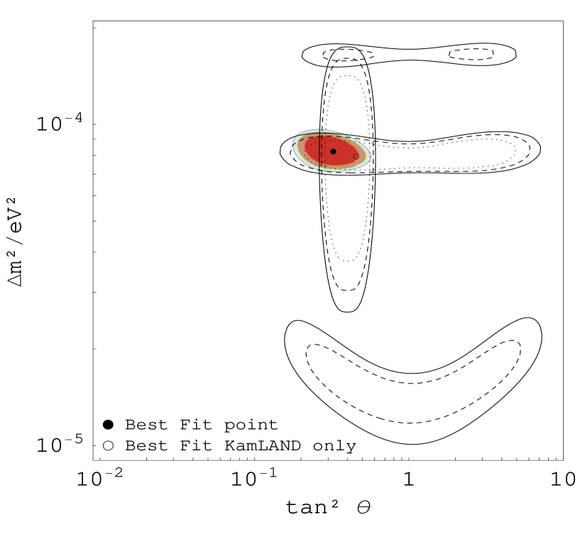
Figure 1: Our best fit $\Delta m^{2}_{21}=8.2\times 10^{-5}eV^{2},~{}tan^{2}\theta=0.31$ (table 3) is superimposed on the neutrino oscillation parameter allowed region from KamLAND [23]. The contour lines are the 95%, 99%, 99.73% CL.

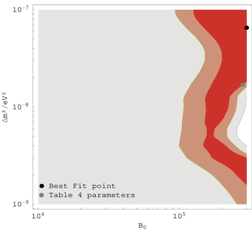
Figure 2: The best fit (table 3) in the plane $\Delta m^{2}_{10},~{}B_{0}$ and the fit of table 4. The contour lines are the 90%, 95%, 99% CL.

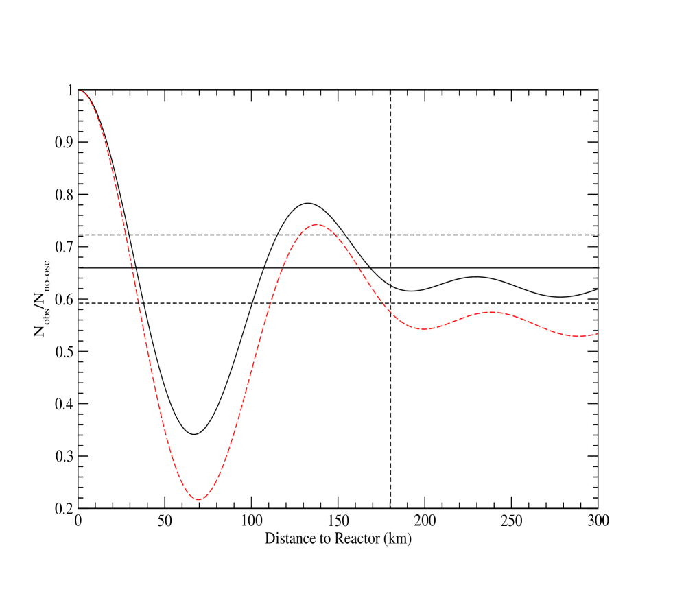
Figure 3: The antineutrino survival probability for the fits considered: LMA (dashed line, table 3) and LMA+SFP ones (full line, tables 3 and 4). Note that the two LMA+SFP fits only differ from each other through the values of $\Delta m^{2}_{10}$ and $B_{0}$ from which the survival probability is independent. Here the straight solid line refers to the central data point (P=0.658) and the two horizontal dashed lines to the 1$\sigma$ range [25]. The effective reactor distance (180km) is marked by the vertical dashed line.

References

- [1] J. N. Bahcall, M. C. Gonzalez-Garcia and C. Pena-Garay, “Solar neutrinos before and after Neutrino 2004,” JHEP 0408 (2004) 016 [arXiv:hep-ph/0406294].
- [2] A. Bandyopadhyay, S. Choubey, S. Goswami, S. T. Petcov and D. P. Roy, “Update of the solar neutrino oscillation analysis with the 766-Ty KamLAND spectrum,” Phys. Lett. B 608, 115 (2005) [arXiv:hep-ph/0406328].
- [3] P. Aliani, V. Antonelli, M. Picariello and E. Torrente-Lujan, “The neutrino mass matrix after Kamland and SNO salt enhanced results,” arXiv:hep-ph/0309156.
- [4] P. Aliani, V. Antonelli, R. Ferrari, M. Picariello and E. Torrente-Lujan, “Analysis of neutrino oscillation data with the recent KamLAND results,” arXiv:hep-ph/0406182.
- [5] B. Aharmim et al. [SNO Collaboration], “A search for periodicities in the B-8 solar neutrino flux measured by the Sudbury Neutrino Observatory,” Phys. Rev. D 72, 052010 (2005) [arXiv:hep-ex/0507079].
- [6] P. A. Sturrock, D. O. Caldwell, J. D. Scargle and M. S. Wheatland, “Power-spectrum analyses of Super-Kamiokande solar neutrino data: Variability and its implications for solar physics and neutrino physics,” Phys. Rev. D 72, 113004 (2005) [arXiv:hep-ph/0501205].
- [7] J. Yoo et al. [Super-Kamiokande Collaboration], “A search for periodic modulations of the solar neutrino flux in Super-Kamiokande-I,” Phys. Rev. D 68 (2003) 092002 [arXiv:hep-ex/0307070].
- [8] P. A. Sturrock and J. D. Scargle, “Histogram analysis of GALLEX, GNO and SAGE neutrino data: Further evidence for variability of the solar neutrino flux,” Astrophys. J. 550, L101 (2001) [arXiv:astro-ph/0011228].
- [9] P. A. Sturrock and D. O. Caldwell, “Power spectrum analysis of the Gallex and GNO solar neutrino data,” arXiv:hep-ph/0409064. Astrophys. J. 605, 568 (2004) [arXiv:hep-ph/0309239].
- [10] D. O. Caldwell and P. A. Sturrock, “New evidence for neutrino flux variability from Super-Kamiokande data,” arXiv:hep-ph/0309191.
- [11] L. B. Okun, M. B. Voloshin and M. I. Vysotsky, “Electromagnetic Properties Of Neutrino And Possible Semiannual Variation Cycle Of The Solar Neutrino Flux,” Sov. J. Nucl. Phys. 44 (1986) 440 [Yad. Fiz. 44 (1986) 677].
- [12] M. B. Voloshin and M. I. Vysotsky, “Neutrino Magnetic Moment And Time Variation Of Solar Neutrino Flux,” Sov. J. Nucl. Phys. 44 (1986) 544 [Yad. Fiz. 44 (1986) 845].
- [13] B. T. Cleveland et al., “Measurement of the solar electron neutrino flux with the Homestake chlorine detector,” Astrophys. J. 496 (1998) 505.
- [14] T. A. Kirsten, “GALLEX solar neutrino results,” Prog. Part. Nucl. Phys. 40 (1998) 85.
- [15] T. Kirsten [GNO collaboration] “Progress in GNO” Talk at Neutrino2002, TU Muenchen, May 2002, Nuclear Physics B (Procceedings Supplements) 118 (2003) 33-38.
- [16] J. N. Abdurashitov et al. [SAGE Collaboration], “Measurement of the solar neutrino capture rate by the Russian-American gallium solar neutrino experiment during one half of the 22-year cycle of solar activity,” J. Exp. Theor. Phys. 95, 181 (2002) [Zh. Eksp. Teor. Fiz. 122, 211 (2002)] [arXiv:astro-ph/0204245].
- [17] V. N. Gavrin [SAGE Collaboration], “Measurement of the solar neutrino capture rate in SAGE and the value of the pp-neutrino flux at the earth,” Nucl. Phys. Proc. Suppl. 138, 87 (2005).
- [18] C. M. Cattadori et al., “Results from radiochemical experiments with main emphasis on the gallium ones, Nucl. Phys. B 143 (2005) (Proc. Suppl.) 3. See also http://neutrino2004.in2p3.fr/.
- [19] B. C. Chauhan and J. Pulido, “LMA and sterile neutrinos: A case for resonance spin flavour precession?,” JHEP 0406 (2004) 008 [arXiv:hep-ph/0402194].
- [20] B. C. Chauhan, J. Pulido and R. S. Raghavan, “Low energy solar neutrinos and spin flavour precession,” JHEP 0507, 051 (2005) [arXiv:hep-ph/0504069].
- [21] B. C. Chauhan, JHEP 0602, 035 (2006) [arXiv:hep-ph/0510415].
- [22] C. Arpesella et al. [BOREXINO Collaboration], “Measurements of extremely low radioactivity levels in BOREXINO,” Astropart. Phys. 18 (2002) 1 [arXiv:hep-ex/0109031].
- [23] T. Araki et al. [KamLAND Collaboration], “Measurement of neutrino oscillation with KamLAND: Evidence of spectral distortion,” Phys. Rev. Lett. 94 (2005) 081801 [arXiv:hep-ex/0406035].
- [24] J. N. Bahcall, A. M. Serenelli and S. Basu, “New solar opacities, abundances, helioseismology, and neutrino fluxes,” Astrophys. J. 621 (2005) L85 [arXiv:astro-ph/0412440].
- [25] K. Eguchi et al. [KamLAND Collaboration], “First results from KamLAND: Evidence for reactor anti-neutrino disappearance,” Phys. Rev. Lett. 90 (2003) 021802 [arXiv:hep-ex/0212021].
- [26] Y. Fukuda et al. [Kamiokande Collaboration], “Solar neutrino data covering solar cycle 22,” Phys. Rev. Lett. 77 (1996) 1683.
- [27] S. Fukuda et al. [Super-Kamiokande Collaboration], “Determination of solar neutrino oscillation parameters using 1496 days of Super-Kamiokande-I data,” Phys. Lett. B 539 (2002) 179 [arXiv:hep-ex/0205075].
- [28] B. Aharmim et al. [SNO Collaboration], “Electron energy spectra, fluxes, and day-night asymmetries of B-8 solar neutrinos from the 391-day salt phase SNO data set,” Phys. Rev. C 72 (2005) 055502 [arXiv:nucl-ex/0502021].
- [29] J. Pulido and E. K. Akhmedov, “Resonance spin flavor precession and solar neutrinos,” Astropart. Phys. 13 (2000) 227 [arXiv:hep-ph/9907399].
- [30] P. Vogel and J. F. Beacom, “The Angular Distribution Of The Neutron Inverse Beta Decay, Anti-Nu/E + P E+ + N,” Phys. Rev. D 60 (1999) 053003 [arXiv:hep-ph/9903554].
- [31] G. L. Fogli, E. Lisi, A. Palazzo and A. M. Rotunno, “Kamland Neutrino Spectra In Energy And Time: Indications For Reactor Power Variations And Constraints On The Georeactor,” Phys. Lett. B 623 (2005) 80 [arXiv:hep-ph/0505081].
- [32] See G. Gratta in Neutrino 2004, http://neutrino2004.in2p3.fr/.
- [33] P. Vogel and J. Engel, “Neutrino Electromagnetic Form-Factors,” Phys. Rev. D 39 (1989) 3378.
- [34] See http://www.awa.tohoku.ac.jp/KamLAND/datarelease/2ndresult.html
- [35] J. Shirai, private communication.