A geometrical scaling solution to the BFKL Pomeron Calculus in the saturation domain

Abstract:

In this paper an analytical solution is found for the BFKL Pomeron calculus in QCD, in which all Pomeron loops have been included. This solution manifests the geometrical scaling behaviour and matches with the solution to the linear evolution equation on the line $r^{2}=1/Q^{2}_{s}(x)$, where $r$ is the dipole size and $Q_{s}$ is the saturation momentum.

1 Introduction

The BFKL Pomeron calculus[1, 2] gives the simplest and the most transparent approach to the high energy amplitude in QCD. This approach is based on the BFKL Pomeron [3] and the interactions between the BFKL Pomerons [4, 5, 6, 7], which are taken into account in the spirit of the Gribov Reggeon Calculus [8]. It can be written in the form of the functional integral (see Ref. [5]) and formulated in terms of the generating functional (see Refs. [9, 10, 11, 12, 13]).

In Ref. [14] (see also Ref. [15]) it is shown that the BFKL Pomeron calculus can be reduced to the following functional integral

$$Z[\Phi,\Phi^{+}]\,\,=\,\,\int\,\,D\,\Phi(b,k;Y)\,D\,\Phi^{+}(b,k;Y)\,e^{S[\Phi,\Phi^{+}]}$$ (1.1)

with

$$S\,\,=\,\,S_{0}\,+\,S_{I}\,\,=\,\,\int\,d^{2}\,b\,d^{2}\,k\,\,\Phi^{+}\left(b,k;Y\right)\,\,\left(\frac{\partial\Phi\left(b,k;Y\right)}{\partial\,Y}\,\,-\,\,\ \frac{\bar{\alpha}_{S}}{2\pi}\,\left(\int\,d^{2}\,k^{\prime}\,K\left(k,k^{\prime}\right)\,\Phi\left(b,k^{\prime};Y\right)\,\,+\right.\right.$$ (1.2)

$$\left.\left.\,\,\Phi^{+}(b,k;Y)\,\Phi(b,k;Y)\,\,\,+\,\,\,\alpha_{S}^{2}\,\left\{\Phi\left(b,k;Y\right)\,\Phi^{+}\left(b,k;Y\right)\,\,-\,\,\Phi^{+}\left(b,k;Y\right)\,\Phi\left(b,k;Y\right)\,\Phi\left(b,k;Y\right)\right\}\,\right)\right)$$

where $K\left(k,k^{\prime}\right)$ is the BFKL kernel in the momentum representation, namely,

$$\int\,d^{2}\,k^{\prime}\,\,K\left(k,k^{\prime}\right)\,\,\Phi\left(b,k^{\prime};Y\right)\,\,=\,\,\int\,d^{2}\,k^{\prime}\,\,\frac{\Phi\left(b,k^{\prime};Y\right)}{(k-k^{\prime})^{2}}\,\,-\,\,k^{2}\,\int\,d^{2}\,k^{\prime}\,\frac{\Phi\left(b,k;Y\right)}{(k-k^{\prime})^{2}\,(k^{\prime 2}\,+\,(k-k^{\prime})^{2})}$$ (1.3)

The theory determined by the functional integral of Eq. (1.1), can be written [14] in the equivalent form introducing the generating functional $Z(Y,[u(b,k)])$ defined as [9]

$$Z\left(Y\,-\,Y_{0};\,[u(b_{i},k_{i})]\right)\,\,\equiv\,\,$$ (1.4)

$$\equiv\,\,\sum_{n=1}\,\int\,\,P_{n}\left(Y\,-\,Y_{0};\,b_{1},k_{1};\dots;b_{i},k_{i};\dots;b_{n},k_{n}\right)\,\,\prod^{n}_{i=1}\,u(b_{i},k_{i})\,d^{2}\,x_{i}\,d^{2}\,k_{i}$$

where $u(b_{i},k_{i})$ are arbitrary functions and $P_{n}\left(Y\,-\,Y_{0};\,b_{1},k_{1};\dots;b_{i},k_{i};\dots;b_{n},k_{n}\right)$ is the probability to find $n$-dipoles with transverse momenta $k_{i}$.

For this functional we have the following evolution equation [14]

$$\frac{\partial\,Z\left(Y-Y_{0};[\,u(b,k)\,]\right)}{\partial\,Y}\,\,=\,\,\chi\,[\,u(b,k)\,]\,\,Z\left(Y-Y_{0};[\,u(b,k)\,]\right)$$ (1.5)

with

$$\chi[u]\,\, = \,\,\,\int\,d^{2}\,b\,d^{2}\,k\,\left(\frac{\bar{\alpha}_{S}}{2\pi}\left(-\int\,d^{2}\,k^{\prime}\,K(k,k^{\prime})u(b,k^{\prime})\,\frac{\delta}{\delta u(b,k^{\prime})}\,+\,u(b,k)\,u(b,k)\,\,\frac{\delta}{\delta u(b,k)}\right)\,-\right.$$ (1.7)

$$\left.-\alpha_{S}^{2}\left(u(b,k)\,u(b,k)\,-\,u(b,k)\right)\,\,\frac{1}{2}\,\frac{\delta^{2}}{\delta u(b,k)\,\delta u(b,k)}\right)\,;$$

In this paper our goal is to solve Eq. (1.5) deeply in the saturation region or, in other words, for the dipoles which sizes are much larger than the typical saturation size $1/Q_{s}(x)$. In the next section we set the problem and will discuss the main assumptions that simplify the problem. In section 3 we discuss the mean field approximation. In this approximation the expression for $\chi[u]$ is simple and it is determined by Eq. (1.7). Solution in this approximation is known (see Ref. [17]) but we will solve this equation using a different method. Therefore, we view this section as a training ground for our method of finding a solution.

In section 4 we focus our efforts on searching a solution to the general equation (see Eq. (1.5)). We consider the solution which shows the geometrical scaling behaviour in the saturation domain and which matches with the linear evolution equation at $r\,\approx\,1/Q_{s}(x)$ where $r$ is the dipole size and $Q_{s}(x)$ is the new scale: saturation momentum.

In conclusions we summarize the main results of the paper and compare them with other attempts to solve this equation .

2 Problem setting and the main assumptions.

The problem that we would like to solve, is the scattering of very small colourless dipole , which size is $r$, with the large target (let say with a nucleus with radius $R$, $R\,\gg\,r$). We are interested in finding the asymptotic behaviour of this amplitude deeply in the saturation region where $\alpha_{S}\ln(r^{2}\,Q^{2}_{s})\,\,\gg\,\,1$.

Generally speaking , we need to fix initial and boundary conditions to solve Eq. (1.5). These conditions are well known and they have the form

Initial conditions: $$\,\,\,\mbox{at }Y=0\,\,\, \,\,\,Z\left(Y=0;[u(b,k)]\right)\,\,=u(b,k)\,\,;$$ (2.8)

Boundary conditions: $$\mbox{at }u_{i}=1 \,\,\,\,\,Z\left(Y;[u(b,k)=1]\right)\,\,\,\,\,=\,\,\,\,\,\,\,\,1\,\,;$$ (2.9)

Eq. (2.8) means that at low energy the interaction can be reduced to the single BFKL Pomeron exchange while Eq. (2.9) follows directly from the meaning of $P_{n}$ as probability to find $n$-dipoles and reflects the normalization for the probability ($\sum P_{n}=1$).

In terms of anomalous dimension $\gamma$ we replace the general BFKL kernel (see solid line in Fig. 1

$$\int\,K(k,k^{\prime})\,e^{(\gamma-1)\,\ln(k^{\prime 2}/k^{2})}\,\,=\,\,\chi\left(\gamma\right)\,\,=\,\,2\,\psi(1)\,\,-\,\,\psi(\gamma)\,\,-\,\,\psi(1-\gamma)$$ (2.10)

by

$$\chi(\gamma)\,\,=\,\,\left\{\begin{array}[]{c}\,\,\,\,\,\,\frac{1}{\gamma}\,\,\hskip 28.45274pt\mbox{for}\,\,r^{2}\,Q^{2}_{s}\,\ll\,1\,;\\ \,\frac{1}{1\,-\,\gamma}\,\,\hskip 28.45274pt\mbox{for}\,\,r^{2}\,Q^{2}_{s}\,\gg\,1\,;\end{array}\right.$$ (2.11)

(see dotted-dashed line in Fig. 1)

This approach is quite different from the diffusion approximation for $\chi\left(\gamma\right)$ (see dotted in Fig. 1

$$\chi\left(\gamma\right)\,\,=\,\,2\ln 2\,\,+\,\,28\,\zeta(3)\,(\gamma-\frac{1}{2})^{2}$$ (2.12)

which was used in Refs. [15, 22, 23, 24] to reduce the general equation to so called Fisher-Kolmogorov-Pertrovsky-Piscounov equation[25] (F-KPP equation). $\zeta(x)$ in Eq. (2.12) is the Riman zeta function.

The kernel of Eq. (2.11) sums the contributions of the order of $\left(\alpha_{S}\,\ln(r^{2}\,\Lambda^{2})\right)^{n}$ for $r^{2}\,Q^{2}_{s}\,\ll\,1$ where $\alpha_{S}\,\ln(r^{2}\,\Lambda^{2})\,\,\gg\,\,1$; and it leads to summation of the terms of the order of $\left(\alpha_{S}\,\ln(r^{2}\,Q^{2}_{s})\right)^{n}$ in the kinematic region where $r^{2}\,Q^{2}_{s}\,\gg\,1$ and $as\,\ln(r^{2}\,Q^{2}_{s})\,\gg\,1$ [16, 17].

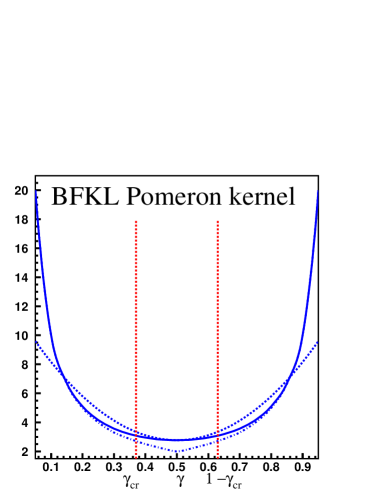
Figure 1: The kernel of the BFKL equation: the solid line shows the exact expression of Eq. (2.10); the kernel of Eq. (2.11) is plotted in dotted-dashed line; and the diffusion approximation of Eq. (2.12) for the BFKL kernel, that leads to F-KPP equation, is presented by dotted line. $\gamma_{cr}$ is calculated using Eq. (2.14).

It means that this kernel can describe the behaviour of our systen deeply in the saturation region ($r^{2}\,Q^{2}_{s}\,\gg\,1$) or/and in the perturbative QCD region at $r^{2}\,Q^{2}_{s}\,\ll\,1$ while we cannot expect that our approximation will be able to reproduce the exact solution in the vicinity of the saturation scale $r^{2}\,Q^{2}_{s}\,\approx\,1$). These features of this kernel one can see from Fig. 1. Fig. 1 shows that the approximate kernel of Eq. (2.11) can describe the exact BFKL kernel only at $\gamma$ close to 0 and 1 while it leads to a contribution which considerably differs from the exact kernel at $\gamma=1/2$. For $\gamma$ close to $1/2$ we can use the diffusion approximation of Eq. (2.12) which fails to reproduce the correct behaviour inside the saturation region. One can see this since we cannot obtain the correct asymptotic behaviour [17] in the mean field approximation with the kernel of Eq. (2.12). On the other hand, the kernel of Eq. (2.11) cannot describe the behaviour of the scattering amplitude in the region close to the saturation scale. In particular, Eq. (2.11) gives the saturation scale as

$$\ln(Q^{2}_{s}\,R^{2})\,\,=\,\,4\bar{\alpha}_{S}\,Y\,\,=\,\,4\bar{\alpha}_{S}\,\ln(1/x)$$ (2.13)

where $\bar{\alpha}_{S}=(N_{c}/\pi)\,\alpha_{S}$, while the correct saturation scale is equal [1, 18, 19]

$$\ln(Q^{2}_{s}\,R^{2})\,\,=\,\,\frac{\chi\left(\gamma_{cr}\right)}{1-\gamma_{cr}}\,\,\,\,\,\mbox{with}\,\,\gamma_{cr}\,\,\mbox{determined by equation:}\,\,\,\,\frac{\chi\left(\gamma_{cr}\right)}{1-\gamma_{cr}}\,\,=\,\,-\,\frac{d\chi\left(\gamma_{cr}\right)}{d\,\gamma_{cr}}$$ (2.14)

Eq. (2.14) gives $\gamma_{cr}=1/2$ that reduces Eq. (2.14) to Eq. (2.13) while the correct value of $\gamma_{cr}$ is $\gamma_{cr}\,=\,0.37$ (see Fig. 1).

We used two additional assumptions to reduce the general functional integral for the BFKL Pomeron calculus given in Ref. [5] to the simple form of Eq. (1.2). Namely, we assume that at high energy we can use the BFKL Pomeron at $\gamma$ close to $1/2$ which leads to

$$\left(L_{12}\,\,\equiv\,\,x^{4}_{12}\nabla^{2}_{x_{1}}\,\,\nabla^{2}_{x_{2}}\right)\,\,G\left(x_{1},x_{2};Y|x^{\prime}_{1},x^{\prime}_{2};Y^{\prime}\right)\,\,=$$

$$=\,\,G\left(x_{1},x_{2};Y|x^{\prime}_{1},x^{\prime}_{2};Y^{\prime}\right)$$ (2.15)

where $G\left(x_{1},x_{2};Y|x^{\prime}_{1},x^{\prime}_{2};Y^{\prime}\right)$ is the Pomeron Green’s function.

This assumption works quite well both for diffusion approximation for the BFKL kernel (see Eq. (2.12)) and for the kernel of Eq. (2.11) since $\gamma_{cr}$ for this kernel is equal to $1/2$ ($\gamma_{cr}=1/2$).

It should be mentioned that Eq. (1.2) is written assuming that

$$b\,\,\equiv\,\,\frac{x_{1}\,+\,x_{2}}{2}\,\,\gg\,\,x_{1}\,-\,x_{2}\,\,;$$ (2.16)

Indeed, this assumption looks natural for the mean field approximation,since we expect that the typical size of the dipoles will be of the order of $1/Q_{s}(x)$ ($Q_{s}(x)$ is the saturation scale) while the typical impact parameter of the scattering dipole should be much larger (at least of the order of the size of a target ($R$) ). However, in the Pomeron loop we have integration over $b$ and we should study the $b$ dependence more carefully. Generally speaking, the integration over impact parameter in the Pomeron loop leads to the value of $b$ of the order the typical size of the dipoles in the loop and can change considerable the conclusions of the approaches where the $b$ dependence has not been taken into account (see [20, 22, 23, 24]).

For our kernel, that sums log contributions, the impact parameter dependence does not influence on such summation since the BFKL Pomeron shows the rapid fall down as a function $b$ ($\propto 1/b^{4}$) and integration over $b$ does not generate any logarithmic contribution. The $b$ dependence for our kernel has been discussed in details in Refs. [1, 17] and we will show how it works in the next section.

It should be mention that the relation between fields in momentum and coordinate representation looks as follows

$$\Phi(x_{1},x_{2};Y)\,\,=\,\,x^{2}_{12}\,\int\,d^{2}\,k\,e^{i\,\vec{k}\cdot\vec{x}_{12}}\,\,\Phi\left(k,b;Y\right)$$ (2.17)

where $x_{12}\,=\,x_{1}-x_{2}$.

We would like to solve directly Eq. (1.5). Our main assumption is that $Z\left(b,k;Y\right)$ actually is a function of one variable $Z\left(\xi;Y,[u]\right)$ :

$$\xi\,\,=\,\,\ln\left(Q^{2}_{s}(x)/k^{2}\right)$$ (2.18)

In finding the solution we replace the generating functional of Eq. (1.4) by the generating function

$$Z\left(\xi,u\right)\,\,\,=\,\,\,\sum_{n=1}\,\,P_{n}\left(\xi\right)\,u^{n}$$ (2.19)

We can use Eq. (2.19) instead of the generating functional of Eq. (1.4) since the scattering amplitude is determined by the following equation [20, 11]

$$N\left(Y;k;[\gamma_{i}]\right) = -\sum^{\infty}_{n=1}\,\frac{(-1)^{n}}{n!}\,\,\gamma_{n}(\{k_{i}\};b;Y_{0};R)\,\,\,\prod^{n}_{i=1}d^{2}k_{i}\,\,\frac{d^{n}}{d^{n}u}Z\left(Y-Y_{0};\{k_{i}\},u\right)|_{u=1}\,\,\rightarrow$$ (2.20)

$$\xrightarrow{\xi\,\gg\,1} -\sum^{\infty}_{n=1}\,\,\,\,\frac{(-1)^{n}}{n!}\,\gamma_{n}(\{k_{i}=1/R\};b;Y_{0};R)\,\,Z\left(Y-Y_{0};\{k_{i}=1/R^{2}\},u\right)|_{u=1}\,\,=$$

$$= -\sum^{\infty}_{n=1}\,\,\,\,\frac{(-1)^{n}}{n!}\,\gamma_{n}(\{k_{i}=1/R\};b;Y_{0};R)\,\,Z\left(\xi;u\right)|_{u=1}\,$$

$\gamma_{n}(\{k_{i}\};b;Y_{0};R)$ in Eq. (2.20) is the scattering amplitude of $n$ dipoles with momenta $k_{i}$ with the target of the size $R$ at low energy. In logarithmic approximation we can consider this amplitude as $\gamma_{n}(\{k_{i}\};b;Y_{0};R)=\gamma_{n}(\{k_{i}=1/R\};b;Y_{0};R)\,\prod^{n}_{i}\,\delta^{(2)}(k_{i}-1/R)$. Therefore we need to know only generating function of Eq. (2.19) to find the scattering amplitude.

In the perturbative QCD region ($r^{2}\,Q^{2}_{s}(x)\,\,\approx\,\,Q^{2}_{s}/k^{\prime 2}\,\,\ll\,\,1$) the scattering amplitude has the following form for the kernel of Eq. (2.11)

$$N\left(Y\,=\,\ln(1/x);\ln(k^{\prime 2}\,R^{2})\right)\,\,=\,\,\alpha_{S}^{2}\,\exp\left(\,2\,\sqrt{\bar{\alpha}_{S}\,Y\,\ln(k^{\prime 2}\,R^{2})}\,\,\,-\,\,\,\ln(k^{\prime 2}\,R^{2})\,\right)$$ (2.21)

which can be translated in the initial condition, namely,

$$Z\left(Y;\ln(k^{\prime 2}\,R^{2});\,u\right)\,\,=\,\,1\,\,\,-\,(1\,-\,u)\,\,\exp\left(\,2\,\sqrt{\bar{\alpha}_{S}\,Y\,\ln(k^{\prime 2}\,R^{2})}\,\,\,-\,\,\,\ln(k^{\prime 2}\,R^{2})\right)$$ (2.22)

In Ref. [26] it is proved that the solution of the linear evolution equation in the vicinity of $k^{2}\to Q^{2}_{s}$ shows the geometrical scaling behaviour and in terms of the generating function this contribution looks as

$$Z\left(\xi;u\right)|_{\xi<0,\,\,|\xi|<1}\,\,=\,\,1\,\,-\,\,(1-u)\,\exp\left(\frac{1}{2}\,\xi\right)$$ (2.23)

for the solution of Eq. (2.22). In Ref. [26] it is shown that the dependence of the perturbative solution on the only one variable $\xi$ is a general property also for the exact kernel of the BFKL equation. Eq. (2.23) will be used as the initial condition in our solution.

To check the strategy of our approach, especially Eq. (2.19) , we first consider the BFKL Pomeron interaction in the kinematic region near to the saturation scale where we expect the geometrical scaling solution of Eq. (2.23). We will show that in leading log approximation of perturbative QCD which corresponds to the kernel of Eq. (2.11), we can avoid the assumptions given by Eq. (2.15) and Eq. (2.16), while Eq. (2.19) will be proved.

3 The BFKL Calculus in the geometrical scaling region

We start with the simplest enhanced diagram of Fig. 2-a. We will write the expression for this diagram for function $\phi$ which is defined as

$$\phi(\xi;\rho,q)\,\,\,=\,\,\,\int\,d^{2}\,b\,\,e^{i\,\vec{q}\cdot\vec{b}}\,\,N\left(\xi,\rho;b\right)$$ (3.24)

where $\xi$ is defined by Eq. (2.18) and $\rho\,\,=\,\,\ln(k^{2}\,R^{2})$. The diagram can be written as follows

$$\phi\left(\mbox{{Fig.~{}\ref{enhdi}}-a}|\xi,\rho;q\right)\,\,=\,\,\int\,d\,\xi^{\prime}d\,\rho^{\prime}d^{2}\,q^{\prime}\,\,d\,\xi"d\,\rho"\,\,\phi\left(\xi-\xi^{\prime},\rho-\rho^{\prime},q\right)\,$$ (3.25)

$$G_{3P}\,,\phi\left(\xi^{\prime}-\xi",\rho^{\prime}-\rho",\vec{q}-\vec{q}^{\prime}\right)\,\,\phi\left(\xi^{\prime}-\xi",\rho^{\prime}-\rho",\vec{q}^{\prime}\right)\,\,G_{3P}\,\,\phi\left(\xi"-\xi_{0},\rho"-\rho_{0},q\right)\,$$

In Eq. (3.25) we introduced the variables $\xi$ instead of rapidity $y$ and $\rho$ instead of $k^{2}$.

The integration over $q^{\prime}$ in Eq. (3.25) has been discussed in details in Refs. [1, 27]. The result of this discussion is the fact that the integration over $q^{\prime}$ sits at $q^{\prime}=$ the lowest virtuality in the loop. In other words, $\int\,d^{2}\,q^{\prime}\,\,=\,\,\pi\,k"^{2}$ in Fig. 2-a if we calculate this diagram in the region of $\xi<0$. Taking this into account we reduce Eq. (3.25) to the following one

$$\phi\left(\mbox{{Fig.~{}\ref{enhdi}}-a}|\xi,\rho;q=0\right)\,\,=\,\,\frac{\alpha_{S}^{2}}{16}\,\,\int^{\xi}\,\,\int^{\rho}\,d\,\xi^{\prime}d\,\rho^{\prime}\,\int^{\xi^{\prime}}\,\,\int^{\rho^{\prime}}\,d\,\xi"d\,\rho"\,\,\phi\left(\xi-\xi^{\prime},\rho-\rho^{\prime},q=0\right)\,$$ (3.26)

$$\,\,\phi\left(\xi^{\prime}-\xi",\rho^{\prime}-\rho",q=0\right)\,\,\phi\left(\xi^{\prime}-\xi",\rho^{\prime}-\rho",q=0\right)\,\,\,\,\phi\left(\xi"-\xi_{0},\rho"-\rho_{0},q=0\right)$$

It is clear the summation all diagrams can be done using the following functional integral

$$Z[\Phi,\Phi^{+}]\,\,=\,\,\int\,\,D\,\Phi(\xi,\rho)\,D\,\Phi^{+}(\xi,\rho)\,e^{S[\Phi,\Phi^{+}]}$$ (3.27)

with

$$S\,\,=\,\,S_{0}\,+\,S_{I}\,\,=\,\,\int\,d\xi\,d\rho\,\Phi^{+}\left(\xi,\rho\right)\,\,\left(4\,\frac{\partial\Phi\left(\xi,\rho\right)}{\,\partial\,\xi}\,\,-\,\,\int^{\rho}\,d\,\rho^{\prime}\,\,\left(\,4\frac{\partial\Phi\left(\xi,\rho^{\prime}\right)}{\,\partial\,\xi}\,\,+\,\,\Phi\left(\xi,\rho^{\prime}\right)\,\,\,+\right.\right.$$ (3.28)

$$\left.\left.\,\,+\,\,\,\Phi^{+}\left(\xi,\rho^{\prime}\right)\,\Phi\left(\xi,\rho^{\prime}\right)+\alpha_{S}^{2}\,\left\{\Phi\left(\xi,\rho^{\prime}\right)\,\Phi^{+}\left(\xi,\rho^{\prime}\right)\,\,-\,\,\Phi^{+}\left(\xi,\rho^{\prime}\right)\,\Phi\left(\xi,\rho^{\prime}\right)\,\Phi\left(\xi,\rho^{\prime}\right)\right\}\,\right)\right)$$

As was shown in Ref.[14] this functional integral can be rewritten as the equation for the generating functional , defined as follows

$$Z\left(\xi,[u(\rho)]\right)\,\,\equiv\,\sum_{n=1}\,\int\,P_{n}\left(\xi,\rho_{1};\dots;\rho_{i};\dots;\rho_{n}\right)\,\prod^{n}_{i=1}u(\rho_{i})\,d\,\rho_{i}$$ (3.29)

namely,

$$4\,\frac{\partial\,Z\left(\xi,[u]\right)}{\partial\xi}\,=$$ (3.30)

$$\,\int\,d\,\rho\,\,\int^{\rho}\,d\,\rho^{\prime}\,\left(\frac{\delta\partial\,Z\left(\xi,[u]\right)}{\delta u[\rho^{\prime}]\,\partial\xi}\,-\,\left(u(\rho)-u(\rho)\,u(\rho^{\prime})\,\right)\,\frac{\delta\,Z\left(\xi,[u]\right)}{\delta u[\rho^{\prime}]}\,\,-\,\,\alpha_{S}^{2}\,\left(u(\rho)\,u(\rho)-u(\rho)\right)\frac{\delta^{2}\,Z\left(\xi,[u]\right)}{\delta u(\rho)\,\delta u(\rho^{\prime})}\right)$$

This functional equation gives the full description in double log approximation for $\xi<0$. In particular, it leads to the linear equation for the functional $N=1-Z\left(\xi,u\,=\,1-\gamma\right)$ if we neglect the terms of the order $N^{2}$. This equation is

$$4\,\left(\frac{\partial^{2}\,N}{\partial\xi\,\partial\,\rho}\,\,+\,\,\frac{\partial\,N}{\partial\xi}\right)\,\,=\,\,N$$ (3.31)

It is easy to check that $N$ of Eq. (2.21) satisfies this equation.

However, Eq. (3.30) can be simplified in the region of $|\xi|\,\gg\,1$ and $\rho\,\gg\,1$ in the kinematic region where we have the geometrical scaling solution of Eq. (2.23). In this region Eq. (3.26) has a simpler form, namely,

$$\phi\left(\mbox{{Fig.~{}\ref{enhdi}}-a}|\xi\right)\,\, =$$

$$= \,\,\frac{\alpha_{S}^{2}}{16}\,\,\int^{\xi}_{\xi_{0}}\,\,d\,\xi^{\prime}\,\int^{\xi^{\prime}}_{0}\,d\,\rho^{\prime}\,\int^{\xi^{\prime}}_{\xi_{0}}\,\,d\,\xi"\,\int^{\xi"}_{0}d\,\rho"\,\,\,\,\phi\left(\xi-\xi^{\prime}\right)\,\,\,\phi\left(\xi^{\prime}-\xi"\right)\,\,\phi\left(\xi^{\prime}-\xi"\right)\,\,\,\,\phi\left(\xi"-\xi_{0}\right)$$ (3.32)

$$= \frac{\alpha_{S}^{2}}{16}\,\,\,\,\,\int^{\xi}_{\xi_{0}}\,\,\xi^{\prime}\,d\,\xi^{\prime}\,\,\int^{\xi^{\prime}}_{\xi_{0}}\,\,\xi"\,d\,\xi"\,\,d\,\xi"\,\int^{\xi"}_{0}d\,\rho"\,\,\,\,\phi\left(\xi-\xi^{\prime}\right)\,\,\,\phi\left(\xi^{\prime}-\xi"\right)\,\,\phi\left(\xi^{\prime}-\xi"\right)\,\,\,\,\phi\left(\xi"-\xi_{0}\right)$$ (3.33)

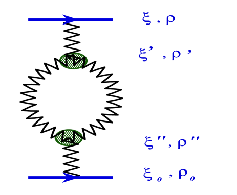
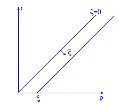
Fig. 2-a	Fig. 2-b

Figure 2: The simplest enhanced diagram for interaction of the BFKL Pomeron (Fig. 2-a) and the plot (Fig. 2-b) for integration variables:  $\xi=4\,\alpha_{S}\,Y\,\,-\,\,\rho$   with $\rho\,\,=\,\,\ln(k^{2}\,R^{2})$. $Y$ is rapidity.

In calculating Eq. (3.32) we restrict ourselves by the kinematic region $\xi<0$ where we can safely use Eq. (2.23) for the BFKL Pomeron. All integrations in Eq. (3.32) and Eq. (3.33) are taken in the so called double log approximation which corresponds to Eq. (2.11) for the kernel and Eq. (2.22) for the solution of the linear equation. We also used the kinematic restriction $\rho<\xi$ that follows from Fig. 2-b.

Eq. (3.33) suggests that the problem of summing all BFKL Pomeron diagrams in the saturation region for $\xi\gg 1$ can be reduced to the solution of the following equation for the generating function defined by Eq. (2.19) and Eq. (2.20)

$$4\,\frac{\partial Z\left(\xi;u\,\right)}{\partial\xi}\,\,\,=\,\,\,-\,\xi\,u\,(1-u)\,\,\frac{\partial Z\left(\xi;u\,\right)}{\partial u}\,\,\,\,+\,\,\,\,\alpha_{S}^{2}\,\,\xi\,\,u\,(1-u)\,\frac{\partial^{2}Z\left(\xi;u\,\right)}{\partial u^{2}}$$ (3.34)

This equation can be rewritten in more convenient form introducing    ${\cal Y}\,=\,\xi^{2}/8$,   namely,

$$\frac{\partial Z\left({\cal Y};u\,\right)}{\partial{\cal Y}}\,\,\,=\,\,\,-\,u\,(1-u)\,\,\frac{\partial Z\left({\cal Y};u\,\right)}{\partial u}\,\,\,\,+\,\,\,\,\,\,\alpha_{S}^{2}\,u\,(1-u)\,\frac{\partial^{2}Z\left({\cal Y};u\,\right)}{\partial u^{2}}$$ (3.35)

Eq. (3.35) is the same as for the BFKL Pomeron calculus in zero transverse dimension (see Ref. [29] and references therein). This equation has been solved [29] . We will discuss below the main propertiers of the solution to Eq. (3.35) but first we start from the solution to our problem in mean field approximation to check the main assumption that we make on the way of obtaining Eq. (3.35).

4 Exact solution and the mean field approximation (MFA)

In the mean field approximation $\chi[u]$ is determined only by Eq. (1.7) . This fact considerably simplifies the equation since such an equation belongs to the well known class of the Louisville equations. The Louisville equation has a general solution, namely, $Z\left(Y-F(u)\right)$. Using this form for the general solution as well as two conditions (initial and boundary, see Eq. (2.8) and Eq. (2.9)): we can easily prove that for $Z$ we have the non-linear equation [9, 10], namely

$$\frac{\partial\,Z\left(Y-Y_{0};b,k\,\right)}{\partial\,Y}\,\,=\,\,\frac{\bar{\alpha}_{S}}{2\pi}\,\left(-\int\,K(k,k^{\prime})\,Z\left(Y-Y_{0};b,k^{\prime}\,\right)\,\,+\,\,Z^{2}\,\left(Y-Y_{0};b,k\,\right)\right)$$ (4.36)

This equation leads to Balitsky-Kovchegov equation[20, 21] for the scattering amplitude and it has been solved in Ref. [17] and the solution turns out to be the function of the only one variable $\xi$ (see Eq. (2.18)). In Ref. [17] it is shown that at large $\xi$ the generating functional $Z\left(Y-Y_{0};b,k^{\prime}\,\right)$ for the kernel of Eq. (2.11) behaves as

$$Z\left(Y-Y_{0};b,k^{\prime}\,\right)\,\,\,=\,\,C\,\exp\left(-\frac{\xi^{2}}{8}\right)$$ (4.37)

In the log approximation for the BFKL kernel in the saturation region which is related to the kernel of Eq. (2.11), (see Ref. [17] and references therein) we have :

$$\int\,d^{2}\,k^{\prime}\,\,K\left(k,k^{\prime}\right)\,\,Z\left(b,k^{\prime};Y\right)\,\,\,\rightarrow\,\,\int^{Q^{2}_{s}(x)}_{k^{2}}\,\,\frac{dk^{2}}{k^{2}}\,\,Z\left(b,k^{\prime};Y\right)$$ (4.38)

In the MFA Eq. (3.35) reduces to very simple Louisville equation, namely

$$\frac{\partial Z\left({\cal Y};u\,\right)}{\partial{\cal Y}}\,\,\,=\,\,\,-\,u\,(1-u)\,\,\frac{\partial Z\left({\cal Y};u\,\right)}{\partial u}$$ (4.39)

which has the solution

$$Z\left({\cal Y};u\,\right)\,\,\,=\,\,\,\frac{u}{1\,\,\,+\,\,\,(1-u)\,\left(\exp\left({\cal Y}\right)\,\,-\,\,1\right)}$$ (4.40)

One can see that Eq. (4.40) satisfies the initial condition of Eq. (2.23) if we define ${\cal Y}\,\,=\,\,\xi^{2}/8\,\,-\,\xi/2$. For $\xi\,\to\,0$ the scattering amplitude is equal to

$$N\left({\cal Y},\gamma=1-u\right)\,\,\,=\,\,\,\frac{\gamma\,\,\exp\left({\cal Y}\right)}{1\,\,\,+\,\,\,\gamma\,\left(\exp\left({\cal Y}\right)\,\,-\,\,1\right)}$$ (4.41)

Since $\gamma$ is of the order of $\alpha_{S}$ we obtain Eq. (2.21) at small $\xi$ with our definition of ${\cal Y}$. Of course, we cannot guarantee term $\frac{1}{2}\xi$ since we assumed that $\xi\,\gg\,1$, therefore, we add this term to guarantee the matching with the initial conditions at $\xi\to 0$.

Therefore, we showed that our procedure involving Eq. (2.19) and Eq. (2.23) leads to the correct behaviour of the amplitude in the mean field approximation. Therefore, we confirm our main assumption that for searching for behaviour at large values of $\xi$, we can consider of generating function of Eq. (2.19) instead of the generating functional of Eq. (1.4).

5 A possible solution with the geometrical scaling behaviour

5.1 General properties

Eq. (3.35) has been solved in Ref. [29]., where it shown that the solution for the scattering amplitude approaches at high energy behaves as

$$N\left(\xi\right)\,\,\,\,\rightarrow\,\,1\,\,-\,\,\exp\left(-C(\kappa)\,\xi^{2}/2\right)$$ (5.42)

Ref. where $\kappa=1/\alpha_{S}^{2}$. The exact value of the factor $C(\kappa)$ is found in Ref. [29], however, here we will illustrate the main property of the exact solution using an approximate semi-classical method developed in Ref. [13] which explores the large value of $\kappa$.

First we find the asymptotic solution to the master equation from the following equation:

$$0\,=\,\,-\,u\,(\,\,-\,\,u)\,\,\frac{\partial Z\left(\xi;u\right)}{\partial u}\,\,\,+\,\,\,\frac{1}{\kappa}\,u\,(1\,\,-\,\,u)\,\frac{\partial^{2}Z\,\left(\xi;u\right)}{\partial u^{2}}$$ (5.43)

The solution that satisfies the boundary condition of Eq. (2.9) is equal to

$$Z_{asymp}\left({\cal Y}=\infty,u\right)\,\,\,=\,\,\,\frac{1\,\,-\,\,e^{\kappa\,u}}{1\,\,\,-\,\,\,e^{\kappa}}$$ (5.44)

The second step is to search the solution in the form

$$Z\left(\xi;u\right)\,\,=\,\,Z_{asymp}\left({\cal Y}=\infty,u\right)\,\,\Delta Z\left(\xi;u\right)$$ (5.45)

assuming that $\partial^{2}\Delta Z\left({\cal Y};u\right)/\partial u^{2}\,\,\ll\,\,\kappa\,\,\left(,\partial Z_{asymp}\left({\cal Y}=\infty,u\right)/\partial u\,\right)\,\left(\partial\Delta Z\left({\cal Y};u\right)/\partial u\right)$. Since $\kappa\,\gg\,1$ this assumption looks reasonable. For $\Delta Z\left(\xi;u\right)$ we obtain the equation

$$\frac{\partial\Delta Z\,\left({\cal Y}u\right)}{\partial\,{\cal Y}}\,\,\,=\,\,\,-\,u\,(1-u)\frac{\partial\Delta Z\,\left({\cal Y}u\right)}{\partial u}\,\,\,+\,\,2\,u(1-u)\,\frac{\partial Z_{asymp}\,\left({\cal Y}=\infty,u\right)}{\partial u}\frac{\partial\Delta Z\,\left({\cal Y}u\right)}{\partial u}$$ (5.46)

Assuming that $\kappa\,\gg\,1$ Eq. (5.46) reduces to the form

$$\frac{\partial\Delta Z\,\left({\cal Y};u\right)}{\partial\,{\cal Y}}\,\,=\,\,\,u\,(1-u)\,\frac{\partial\,\Delta Z\,\left({\cal Y};u\right)}{\partial u}$$ (5.47)

Eq. (5.47) has the solution

$$\Delta Z\,\left({\cal Y};u\right)\,\,\,=\,\,\Phi\left(\,{\cal Y}\,+\,\ln(\frac{u}{1-u}\right)$$ (5.48)

with function $\Phi$ that should be found from the initial conditions of Eq. (2.8).

The solution is

$$Z_{asymp}\left({\cal Y}=\infty;u\right)\,\Delta Z\,\left({\cal Y};u\right)\,\,\,=\,\,\,\tilde{u}\frac{1\,-\,e^{\kappa\,u}}{1\,-\,e^{\kappa\,\tilde{u}}}\,\,\,\,\,\mbox{with}\,\,\,\,\,\,\tilde{u}\,\,\,=\,\,\,\frac{u}{u\,\,+\,\,(1-u)\,\exp\left(-{\cal Y}\right)}$$ (5.49)

However we cannot use directly Eq. (5.49) to determine the asymptotic behaviour of the scattering amplitude at high ${\cal Y}$ since we need to find the typical values of $u$ for such an amplitude at large values of $\xi$ or to find the solution in the entire kinematic region. The latter we cannot do since our equation is valid only at $\xi\,\gg\,1$. To solve this problem at $\xi\,\gg\,1$ we need to use the $t$=channel unitarity constraints ( see Refs. [33, 34, 13]). we need to use the $t$-channel unitarity constraint ( see Refs. [33, 34, 13]), which has the following form

$$N^{MPSI}\left(\xi\right)\,\,\,=\,\,\sum_{n=1}^{\infty}\,\,\frac{(-1)^{n}}{\,n!\,}\,\,\frac{\delta^{n}Z\left(\xi\,-\,\xi^{\prime};u\right)}{\delta u^{n}}|_{u=1}\,\frac{\delta^{n}Z\left(\xi^{\prime};v\right)}{\delta v^{n}}|_{v=1}\,\gamma^{BA}$$ (5.50)

where $\gamma^{BA}$ is the amplitude in the Born approximation for the interaction of two dipoles at low energy, which is equal to $\alpha_{S}^{2}=1/\kappa$ in our case. Using $\kappa\,\gg\,1$ we see that in this limit $\frac{d^{n}Z}{du^{n}}=\left(\kappa\frac{d\tilde{u}}{du}\right)^{n}Z$ and $\frac{d\tilde{u}}{du}\,=\,\exp\left(-{\cal Y}\right)$ at $u=1$.

Using these observation we obtain that

$$N^{MPSI}\left(\xi\right)\,\,\, \xrightarrow{\xi\,\gg\,1} \,\,1\,\,-\,\,\exp\left\{-\,\alpha_{S}^{2}\,\kappa^{2}\,\left(\,1\,\,-\,\,e^{-\frac{(\xi-\xi^{\prime})^{2}}{8}}\,\right)\,\left(\,1\,-\,\,e^{-\,\frac{\xi^{\prime 2}}{8}}\right)\right\}\,\,$$ (5.51)

$$\xrightarrow{\xi\,\gg\,1,\xi^{\prime}=1/2\xi} \,\,1\,-\,e^{-\alpha_{S}^{2}\kappa^{2}}\,\,-\,\,2\kappa\,\,e^{-\xi^{2}/32}$$

The choice $\xi^{\prime}=\xi/2$ is clear since it gives the slowest approach to $N=1$. Eq. (5.51) can only be considered as a approximation to the exact solution of Ref.[29] . It should be stressed that Eq. (5.51) leads to quite a diffrent result in comparison with the Mueller-Patel-Salam-Iancu approach [33]. However, the MPSI approach has an advantage to be correct also for $\xi\approx 1$. This is the reason why we consider our problem in this approach in the next section.

5.2 The Mueller-Patel-Salam-Iancu (MPSI) approach

This approximation has a legitimate region of applicability [33, 34]; can be used for small values of $\xi$ and it describes quite well in the entire kinematic region the exact solution to the BFKL Pomeron calculus in zero transverse dimension [35].

In this approach the scattering amplitude can be calculated using the following formula [33, 34]

$$N^{MPSI}\left(x,y;x^{\prime},y^{\prime};Y\right)\,\,\,=$$ (5.52)

$$\,\,\sum_{n=1}^{\infty}\,\,(-1)^{n}\,n!\,\int\prod^{n}_{i=1}\,d\,x_{i}\,d\,y_{i}\,d\,x^{\prime}_{i}d\,y_{i}\frac{\delta^{n}Z^{MFA}\left(Y-Y^{\prime};[u_{i}]\right)}{\delta u^{n}_{i}}|_{u_{i}=1}\,\frac{\delta^{n}Z^{MFA}\left(Y^{\prime};[v_{i}]\right)}{\delta v^{n}_{i}}|_{v_{i}=1}\,\gamma^{BA}(x_{i},y_{i};x^{\prime}_{i},y^{\prime}_{i})$$

where $\gamma^{BA}(x_{i},y_{i};x^{\prime}_{i},y^{\prime}_{i})$ is the amplitude of interaction of two dipoles in the Born approximation of perturbative QCD.

In the case of the geometrical scaling solution the MPSI approximation formula has an elegant form [36], namely

$$N^{MPSI}\left(\xi\right)\,\,\,=\,\,\,1\,\,\,-\,\,\left\{\exp\left(-\gamma\,\frac{d}{du}\,\frac{d}{dv}\right)\,N^{MFA}\left(\xi-\xi^{\prime};u\right)\,N^{MFA}\left(\xi^{\prime},v\right)\,\right\}|_{u=1;v=1}$$ (5.53)

where the generating function $\,N^{MFA}\left(\xi,u\right)$ is defined as

$$N^{MFA}\left(\xi,u\right)\,\,\,=\,\,1\,\,-\,\,Z^{MFA}\left(\xi,u\right)$$ (5.54)

The generating functional in MFA for the kernel of Eq. (2.11) has been found in Ref. [17]. In this paper it is shown that the solution to Eq. (4.36) has the form that in our notations looks as follows

$$N\left(\xi,\gamma\equiv 1-u\right)\,\,\,=\,\,\,1\,\,\,-\,\,\exp\left(-\zeta(\xi,u)\right)$$ (5.55)

where function $\zeta(\xi,u)$ can be calculated from the implicit equation

$$\xi\,\,=\,\,\sqrt{2}\,\int^{\zeta}_{\gamma}\,\,\frac{d\,\zeta^{\prime}}{\sqrt{\zeta^{\prime}\,\,+\,\,\left(\exp(-\zeta^{\prime})\,-\,1\right)}}$$ (5.56)

For small values of $\zeta\to\gamma$ Eq. (5.56) gives

$$\ln\left(\zeta(\xi,u)/\gamma\right)\,\,\,=\,\,\frac{1}{2}\,\xi\,\,\,\,\mbox{which leads to}\,\,\,\,\zeta(\xi,u)\,\,=\,\,\gamma e^{\frac{\xi}{2}}\,\,\,\xrightarrow{\xi\,\ll\,1}\,\,\,\gamma\,\left(1+\frac{\xi}{2}\right)$$ (5.57)

It is easy to see that Eq. (5.55) with $\zeta(\xi,u)$, determined by Eq. (5.57), satisfies the initial conditions of Eq. (2.23), namely,

$$N\left(\xi=0,\gamma\right)\,\,=\,\,\gamma\,\,\,\,\,\,\,\,\,\,\,\,\mbox{and}\,\,\,\,\,\,\,\,\,\,\,\,\frac{d\,\ln N\left(\xi,\gamma\right)}{d\,\xi}|_{\xi=0}\,\,=\,\,\frac{1}{2}$$ (5.58)

For large $\zeta$ Eq. (5.56) leads to

$$\zeta(\xi,u)\,\,=\,\,\frac{\xi^{2}}{8}$$ (5.59)

which does not depend on $u$. Using this limiting behaviour we can suggest the following extrapolation formula

$$\xi\,\, = \,\,\,\,\sqrt{2}\,\int^{\zeta}_{\gamma}\,\,d\,\zeta^{\prime}\left(\frac{1}{\sqrt{\zeta^{\prime}\,\,+\,\,\left(\exp(-\zeta^{\prime})\,-\,1\right)}}\,\,-\,\,\frac{\sqrt{2}}{\zeta^{\prime}}\right)\,\,+\,\,2\,\ln(\zeta/\gamma)$$ (5.60)

$$= \,2\,\sqrt{2\,\zeta}\,\,\,+\,\,\,2\,\ln(\zeta/\gamma)$$ (5.61)

In the first integral in Eq. (5.60) the small values of $\zeta^{\prime}$ does not contribute and we can replace it by the asymptotic al behaviour at large $\zeta^{\prime}$.

Using Eq. (5.57),Eq. (5.59) and Eq. (5.61) we can suggest an approximation for the solution of Eq. (5.56), namely.

$$\zeta\left(\xi;\gamma\right)\,\,\,=\,\,\,\gamma(1+\xi/2)\,\,+\,\,\xi^{2}/8$$ (5.62)

Substituting Eq. (5.62) into Eq. (5.53) and choosing $\xi^{\prime}=\xi/2$ that correspond to the smallest corrections (see [33] ) , we obtain the final result

$$N^{MPSI}\left(\xi\right)\,\,\,=\,\,\,1\,\,\,\,-\,\,\,\exp\left(-\,\xi^{2}/16\,\,-\gamma\,(1\,+\,\xi/2)\right)$$ (5.63)

Therefore, the MPSI approximation leads to the geometrical scaling which satisfies the initial conditions at $\xi=0$. The $\xi^{2}$ term does not depend of the scattering amplitude $\gamma\propto\alpha_{S}^{2}$ while the next terms show such dependence. Comparing with the solution of Eq. (5.51) one can see that both have the same $\xi^{2}$ dependence but the coefficients in front of of this term is quite different. We need to recall that the MPSI approach cannot be correct at very high energies [33].

6 Conclusions

The main result of this paper is the reduction of the complicated problem of summing all Pomern loops to a Pomeron calculus in the zero transverse dimension but for ’time’ ${\cal Y}$ given by ${\cal Y}=\xi^{2}/8$ at $\xi\,\gg\,1$. The principle features of this solution is the fact that the scattering amplitude depends on the only one variable: $Q^{2}_{s}(x)\,r^{2}$ where $Q_{s}(x)$ is the saturation scale while $r$ is the size of the scattering dipole. Such geometrical scaling behaviour has been proven for the mean field approximation and has been seen experimentally [31]. However, this scaling behaviour was not expected for the theory given by the functional integral of Eq. (1.1). Indeed, at first sight, such theory can be rewritten as the Langevin equation for directed percolation [32], namely,

$$\frac{\partial\,\,\Phi\left(b,k;Y\right)}{\partial Y}\,\,\,=\,\,\frac{\bar{\alpha}_{S}}{2\pi}\,\int\,d^{2}\,k^{\prime}\,K\left(k,k^{\prime}\right)\,\Phi\left(b,k^{\prime};Y\right)\,\,\,-\,\,\,\frac{2\,\pi\,\bar{\alpha}_{S}^{2}}{N_{c}}\cdot\,\Phi(b,k;Y)\,\Phi(b,k;Y)\,\,+\,\,\zeta(b,k;Y)$$ (6.64)

with

$$<|\zeta(b,k;Y)|>\,\,=\,\,0\,;$$ (6.65)

$$\,\,\,\,\,\,\,\,\,\,\,<|\zeta(b,k;Y)\,\zeta(b^{\prime},k^{\prime};Y^{\prime})|>\,\,=\,\,\frac{4\,\pi\,\bar{\alpha}_{S}^{2}}{N_{c}}\cdot\Phi(b,k;Y)\,\left(1-\Phi(b,k;Y)\right)\,\,\delta^{(2)}(\vec{b}-\vec{b}^{\prime})\,\,k^{2}\,\delta^{(2)}(\vec{k}-\vec{k}^{\prime})\,\,\delta\left(Y-Y^{\prime}\right)$$

As it has been shown in Refs. [22, 23, 24] we rather expect from the statistical physics analogy a solution of the following type

$$N\left(\tilde{\xi};Y\right)\,\,=\,\,\frac{1}{\sqrt{2\pi}\,\sigma(Y)}\,\int d\ln(Q^{2}_{s}\,R^{2})\,\,N\left(\ln(Q^{2}_{s}/k^{2})\right)\,\,\exp\left(-\frac{\left(\ln(Q^{2}_{s}\,R^{2})\,\,-\,\,<\ln(Q^{2}_{s}\,R^{2})>\right)^{2}}{2\,\sigma^{2}(Y)}\right)$$ (6.66)

where $N\left(\ln(Q^{2}_{s}/k^{2})\right)$ is the scaling solution in the mean field approximation; $<\ln Q^{2}_{s}>$ is the average saturation scale which differs from $Q_{s}$ given by Eq. (2.13) or Eq. (2.14), namely,[22]

$$<\ln(Q^{2}_{s}\,R^{2})>\,\,=\,\,\ln(Q^{2}_{s}\,R^{2})\,\,\,-\,\,\frac{\pi^{2}\bar{\alpha}_{S}}{2}\,\frac{\gamma_{cr}\,\chi^{\prime\prime}(\gamma_{cr})}{\ln^{2}(1/\alpha_{S}^{2})}\,Y$$ (6.67)

and variance of the saturation momentum $\sigma$ is proportional to

$$\sigma^{2}\,\,=\,\,<\ln^{2}(Q^{2}_{s}\,R^{2})>\,\,-\,\,(<\ln(Q^{2}_{s}\,R^{2})>)^{2}\,\,\propto\,\,\frac{\bar{\alpha}_{S}}{\ln^{3}(1/\alpha_{S}^{2})}\,Y$$ (6.68)

The Pomeron loops change drastically the geometrical scaling behaviour of the MFA solution in an obvious contradiction with our solution. Indeed, Eq. (6.66) means that the amplitude is a function of one variable

$$N\left(\tau\right)\,\,\,=\,\,\,N\left(\frac{\ln(k^{2}\,R^{2})\,\,-\,\,<\ln(Q^{2}_{s}(Y)\,R^{2})>}{\sqrt{\bar{\alpha}_{S}\,Y/\ln^{3}(1/\alpha_{S}^{2})}}\right)$$ (6.69)

Despites that Eq. (6.69) looks very plausible we should not forget that it is correct for the functional integral of Eq. (1.2) which does not treat the impact parameter behaviour in consistent way. As has been demonstrated in section 3 Eq. (2.16), which is needed for a proof of Eq. (1.2), cannot be valid in the Pomeron loops.

The reason for such difference between our approach and Eq. (6.69) is clear from the consideration in section 3: we found that not all Pomeron loops lead to a violation of the geometrical scaling behaviour. Some of them contribute to a change of the scaling solution in the MFA.

In our approach we have the following equation for the directed percolation instead of Eq. (6.64)

$$4\,\frac{\partial\,\,\Phi\left(\xi\right)}{\partial\xi}\,\,\,=\,\,\xi\Phi\left(\xi^{\prime}\right)\,\,\,-\,\,\,\frac{2\,\pi\,\bar{\alpha}_{S}^{2}}{N_{c}}\cdot\,\xi\,\Phi(\xi)\,\Phi(\xi)\,\,+\,\,\zeta(\xi)$$ (6.70)

with

$$<|int\,\zeta(\xi)|>\,\,=\,\,0\,;$$ (6.71)

$$\,\,\,\,\,\,\,\,\,\,\,<|\zeta(\xi)\,\zeta(\xi^{\prime})|>\,\,=\,\,\frac{4\,\pi\,\bar{\alpha}_{S}^{2}}{N_{c}}\cdot\,\,\xi\,\Phi(\xi)\,\left(1-\Phi(\xi)\right)\,\,\delta(\xi-\xi^{\prime})$$

These equations are equivalent to one dimensional Pomeron theory. The first and, perhaps, the only that this theory does, it leads to replacement of the MFA solution in Eq. (6.66) by the solution that has been discussed here. Eq. (6.71) suggests that the correlation term in Eq. (6.65) has a more complicated structure. We propose to sum Eq. (6.71) and Eq. (6.65) but , at the moment, we do not understand the correct $b$ dependence in Eq. (6.65).

We would like to stress that we suggest a solution only for $\xi\,\gg\,1$ and matching with the initial conditions was done in an approximate approach (the MPSI approach). Therefore, in principle, could be that the solution we advocate here, just a wrong one but we believe that the MPSI approximation works well enough to be an argument against such a possibility.

On the other hand, Eq. (6.66) is proven only in the vicinity of the saturation scale where, indeed, $N\left(\ln(Q^{2}_{s}/k^{2})\right)$ is the solution for MFA which is averaged with a Gaussian weight. However, it is difficult to understand how Eq. (6.69) can be matched with the perturbative QCD solution of Eq. (2.22) or Eq. (2.23) outside the saturation kinematic region. Indeed, $\partial\ln N/\partial\ln(k^{2}\,R^{2})=(1/\sigma(Y))\,d\ln N/d\tau\,\,\ll\,1$ instead of $\partial\ln N/\partial\ln(k^{2}\,R^{2})\,\approx\,1$.

At first sight the numerical calculation in Refs. [15, 22, 23, 24, 37] can give us an information on how the solution behaves deeply inside of the saturation region. However, it is not the case at the moment , since: (i) all calculations have been performed for the diffusion kernel of Eq. (2.12) (in other words, for the F-KPP equation) that cannot pretend to describe approaching to the asymptotic behaviour; (ii) the hope that such calculation can be generalized to the exact BFKL kernel is based on some conditions (see Rev. [37]) which are plausible only in vicinity of the saturation scale; (iii) it has not been checked that the numerical solution reproduces the solution of Eq. (2.22) or Eq. (2.23) , rather from fig. 16 of Rev.[37] one can conclude that they do not approach them; and (iv) the accuracy of the numerical calculations has not been checked by a comparison with the exactly solved model of the BFKL Pomeron calculus in zero transverse dimension. For the BFKL Pomeron calculus in zero transverse dimension the numerical calculation should coinside with the exact solution given in Ref. [29] with Eq. (6.65) and should lead to decreasing amplitude at high energy (see Ref.[38] and references therein) for Eq. (6.65) without $\Phi^{2}(b,k;Y)$ term.

It should be stressed that the experimental data do not show any deviation from the geomerical scaling behaviour while the estimates with $\alpha_{S}\approx 0.25$ show that we expect a considerable violation of this scaling behaviour accordingly to Eq. (6.66).

Summarising we do not think that there is any proof that our solution is inconsistent but , of course, we need to remember that this solution cannot be justified in the vicinity of the saturation scale. The only that we showed is that our solution does not contradict the exact solution in the perturbative QCD region (see Eq. (2.22) or Eq. (2.23)). Such strategy was successful in the case of the mean field approximation [17]. On the other hand, solution of Eq. (6.66) is able to describe the system in the vicinity of the saturation scale but it is not hundred percents clear how this solution could be matched with Eq. (2.22) or Eq. (2.23). We would like to stress again that the most probable way out is that we need to replace the MFA solution by ours in Eq. (6.66).

We are working to include the exact BFKL kernel in our consideration and to understand better the kinematic region of matching with the perturbative QCD solution. This is a very important issue since the model kernel of Eq. (2.11) does not give a correct high energy solution in the MFA (see Ref. [28]). If we will use the correct solution in the MPSI approximation we will obtain the solution which being substituted in Eq. (6.66) leads to a geometrical scaling behaviour after integration over $\ln(Q^{2}_{s}\,R^{2})$ . The only change is to replace $Q^{2}_{s}$ in the definition of variable $\xi$ (see Eq. (2.18)) by the new saturation momentum of Eq. (6.67).

We hope that the paper will be useful    in searching a solution in the saturation region beyond the scope of statistical physics analogy for the BFKL Pomeron calculus including the Pomeron loops.

References

• [1] L. V. Gribov, E. M. Levin and M. G. Ryskin, Phys. Rep.100, 1 (1983).
• [2] A. H. Mueller and J. Qiu, Nucl. Phys.,427 B 268 (1986) .
• [3] E. A. Kuraev, L. N. Lipatov, and F. S. Fadin, Sov. Phys. JETP 45, 199 (1977);     Ya. Ya. Balitsky and L. N. Lipatov, Sov. J. Nucl. Phys.28, 22 (1978).
• [4] J. Bartels, M. Braun and G. P. Vacca, Eur. Phys. J. C40, 419 (2005) [arXiv:hep-ph/0412218] ;    J. Bartels and C. Ewerz, JHEP 9909, 026 (1999) [arXiv:hep-ph/9908454] ;    J. Bartels and M. Wusthoff, Z. Phys. C66, 157 (1995) ;        A. H. Mueller and B. Patel, Nucl. Phys. B425, 471 (1994) [arXiv:hep-ph/9403256];    J. Bartels, Z. Phys.  C60, 471 (1993).
• [5] M. A. Braun, Phys. Lett.B632 (2006) 297 [arXiv:hep-ph/0512057];   arXiv:hep-ph/0504002 ; Eur. Phys. J. C16, 337 (2000) [arXiv:hep-ph/0001268];    M. Braun, Eur. Phys. J. C6, 321 (1999) [arXiv:hep-ph/9706373];    M. A. Braun and G. P. Vacca, Eur. Phys. J. C6, 147 (1999) [arXiv:hep-ph/9711486].
• [6] H. Navelet and R. Peschanski, Nucl. Phys. B634, 291 (2002) [arXiv:hep-ph/0201285];     Phys. Rev. Lett. 82, 137 (1999), [arXiv:hep-ph/9809474];    Nucl. Phys.  B507, 353 (1997) [arXiv:hep-ph/9703238].
• [7] J. Bartels, L. N. Lipatov and G. P. Vacca, Nucl. Phys. B706, 391 (2005) [arXiv:hep-ph/0404110].
• [8] V. N. Gribov, Sov. Phys. JETP 26, 414 (1968) [Zh. Eksp. Teor. Fiz. 53, 654 (1967)].
• [9] A. H. Mueller, Nucl. Phys. B415, 373 (1994); ibid B437, 107 (1995).
• [10] E. Levin and M. Lublinsky, Nucl. Phys.A730, 191 (2004) [arXiv:hep-ph/0308279].
• [11] E. Levin and M. Lublinsky, Phys. Lett. B607, 131 (2005) [arXiv:hep-ph/0411121].
• [12] E. Levin and M. Lublinsky, Nucl. Phys. A763,172 (2005) , arXiv:hep-ph/0501173.
• [13] E. Levin, Nucl. Phys. A763, 140 (2005), arXiv:hep-ph/0502243.
• [14] M. Kozlov, E. Levin and A. Prygarin, “The BFKL pomeron calculus: Probabilistic interpretation and high energy amplitude,” arXiv:hep-ph/0606260.
• [15] C. Marquet, G. Soyez and B. W. Xiao, “On the probability distribution of the stochastic saturation scale in QCD,” arXiv:hep-ph/0606233.
• [16] A. H. Mueller, Nucl. Phys.  B558 (1999) 285, [arXiv:hep-ph/9904404].
• [17] E. Levin and K. Tuchin, Nucl. Phys.  A693 (2001) 787 [arXiv:hep-ph/0101275];   A691 (2001) 779 [arXiv:hep-ph/0012167];   B573 (2000) 833 [arXiv:hep-ph/9908317].
• [18] A. H. Mueller and D. N. Triantafyllopoulos, Nucl. Phys.  B640 (2002) 331 [arXiv:hep-ph/0205167];    D. N. Triantafyllopoulos, Nucl. Phys. B 648 (2003) 293 [arXiv:hep-ph/0209121]
• [19] S. Munier and R. Peschanski, Phys. Rev.  D70 (2004) 077503; D69 (2004) 034008 [arXiv:hep-ph/0310357];   Phys. Rev. Lett.91 (2003) 232001 [arXiv:hep-ph/0309177].
• [20] Y. V. Kovchegov, Phys. Rev. D60, 034008 (1999), [arXiv:hep-ph/9901281].
• [21] Ia. Balitsky, Nucl.  Phys. B463 (1996) 99.
• [22] E. Iancu, A. H. Mueller and S. Munier, Phys. Lett. B 606 (2005) 342 [arXiv:hep-ph/0410018]; E. Brunet, B. Derrida, A. H. Mueller and S. Munier, “Noisy traveling waves: effect of selection on genealogies,” arXiv:cond-mat/0603160; Phys. Rev.E73 (2006) 056126 [arXiv:cond-mat/0512021].
• [23] R. Enberg, K. Golec-Biernat and S. Munier, Phys. Rev.  D72 (2005) 074021 [arXiv:hep-ph/0505101].
• [24] E. Iancu and D. N. Triantafyllopoulos, Nucl. Phys. A 756 (2005) 419 [arXiv:hep-ph/0411405]; G. Soyez, Phys. Rev. D 72 (2005) 016007 [arXiv:hep-ph/0504129]; E. Iancu, C. Marquet and G. Soyez, “Forward gluon production in hadron hadron scattering with Pomeron loops,” arXiv:hep-ph/0605174.
• [25] B.A. Fisher, Ann. Eugenenics 7, 355 (1937); A. Kolmogorov, I. Petrovsky and N. Piscounov, Moskou Univ. Bull. Math. A1,1 (1937).
• [26] E. Iancu, K. Itakura and L. McLerran, Nucl. Phys. A 708 (2002) 327 [arXiv:hep-ph/0203137].
• [27] E. Levin and M. Wusthoff, Phys. Rev. D 50 (1994) 4306.
• [28] M. Kozlov and E. Levin, Nucl. Phys.  A764 (2006) 498 [arXiv:hep-ph/0504146].
• [29] M. Kozlov and E. Levin, “Solution for the BFKL pomeron calculus in zero transverse dimensions,” arXiv:hep-ph/0604039.
• [30] D. Amati, M. Le Bellac, G. Marchesini and M.Ciafaloni, Nucl. Phys. B112 (1976) 107;
D. Amati, G. Marchesini, M.Ciafaloni and G. Parisi, Nucl. Phys. B114 (1976) 483.
• [31]  J. Kwiecinski and A. M. Stasto, Acta Phys. Polon.B33 (2002) 3439;  Phys. Rev.D66 (2002) 014013 [arXiv:hep-ph/0203030];     A. M. Stasto, K. Golec-Biernat and J. Kwiecinski, Phys. Rev. Lett.86 (2001) 596 arXiv:hep-ph/0007192];    J. Bartels and E. Levin, Nucl. Phys. B387 (1992) 617;   E. Iancu, K. Itakura and L. McLerran, Nucl. Phys.A708 (2002) 327 [arXiv:hep-ph/0203137].
• [32] H. Hinrichsen, Advances in Physics 49 815 (2000).
• [33] E. Iancu and A. H. Mueller, Nucl. Phys.A730 (2004) 460, 494, [arXiv:hep-ph/0308315],[arXiv:hep-ph/0309276].
• [34] M. Kozlov and E. Levin, Nucl. Phys.  A739 (2004) 291 [arXiv:hep-ph/0401118]
• [35] M. Kozlov, E. Levin, V. Khachatryan and J. Miller, arXiv:hep-ph/0610084.
• [36] Y. V. Kovchegov, Phys. Rev. D 72 (2005) 094009 [arXiv:hep-ph/0508276].
• [37] G. Soyez, “QCD at high energy: Saturation and fluctuation effects,” arXiv:hep-ph/0610436.
• [38] S. Bondarenko, L. Motyka, A. H. Mueller, A. I. Shoshi and B. W. Xiao, “On the equivalence of Reggeon field theory in zero transverse dimensions and reaction-diffusion processes,” arXiv:hep-ph/0609213.