SPhT-T06/093.

On-shell Recursion Relations for n-point QCD

Darren Forde.

Service de Physique Théorique, CEA–Saclay
F–91191 Gif-sur-Yvette cedex, France

We present on the use of on-shell recursion relations. These can be used not only for calculating tree amplitudes, including those with masses, but also to compute analytically the missing rational terms of one-loop QCD amplitudes. Combined with the cut-containing pieces calculated using a unitarity approach complete one-loop QCD amplitudes can be derived. This approach is discussed in the context of the adjacent 2-minus all-multiplicity QCD gluon amplitude.

1 Introduction

The forthcoming experimental program at CERN’s Large Hadron Collider will place new demands on theoretical calculations. In order to reach the precision required by searches for and measurements of new physics, these processes need to be computed to next-to-leading order (NLO), which entails the computation of one-loop amplitudes. These are challenging calculations. State-of-the-art Feynman-diagrammatic computations have only recently reached six-point amplitudes [1] due to the large numbers of diagrams involved.

Feynman diagram techniques are not the only method for performing these needed one-loop contributions. Within the unitarity-based method [2, 3, 4] and related recent developments [5, 6], one can decompose one-loop colour-ordered gluonic QCD amplitudes into pieces corresponding to ${\cal N}=4$, ${\cal N}=1$, and scalar contributions as $A_{n}=A_{n}^{{\cal N}=4}-4A_{n}^{{\cal N}=1}+A_{n}^{\rm scalar}$. The supersymmetric contributions can be computed by performing the cut algebra strictly in four dimensions, with only the loop integrations computed in $D=4-2\epsilon$ dimensions. Scalar-loop contributions require that the cut algebra, and the corresponding tree amplitudes fed into the unitarity machinery, also be computed in $D=4-2\epsilon$ dimensions [4, 7, 8]. This makes the computation of these pieces somewhat more difficult than in the supersymmetric case and leads us to desire a more efficient approach.

At one loop, computing a scalar loop in $D=4-2\epsilon$ dimensions is equivalent to computing a massive scalar loop in $D=4$ dimensions, and then integrating over the mass with an appropriate weighting. The computation of tree-level amplitudes with massive scalars is thus of use in the unitarity method for computing massless loop amplitudes in non-supersymmetric gauge theories. On-shell recursion relations can be applied to calculate the necessary tree amplitudes [9, 10]. These relations extend the tree-level on-shell recursion relations of Britto, Cachazo, Feng, and Witten [11]. The remarkable generality and simplicity of the proof of these recursion relations, requiring only Cauchy’s theorem and a knowledge of the factorisation properties of the amplitudes, has enabled widespread application at tree level [12] and even at loop level [13, 14, 15].

Using massive scalars, although more straightforward than the unitarity method in $D=4-2\epsilon$ dimensions, is still not the most efficient applicable technique. More efficient still is an updated version of the unitarity bootstrap technique [5]. This technique relies on first obtaining the cut-constructible parts of a desired amplitude — those terms containing polylogarithms, logarithms, and associated $\pi^{2}$ terms — via the unitarity method in $D=4$. The missing rational terms that this process cannot capture are then derived using one-loop on-shell recursion relations [14]. This allows for a practical and systematic construction of the rational terms of loop amplitudes.

2 Recursive Bootstrap Approach

Before describing the extension of the on-shell recursion relations to loop processes we first give an overview of the tree level recursion relations including their application to massive theories. In the simplest case the recursion relations employ a parameter-dependent ‘$[j,l\rangle$’ shift of two of the external massless spinors, $j$ and $l$, in an $n$-point process,

$$[j,l\rangle:\qquad {\tilde{\lambda}}_{j} \rightarrow{\tilde{\lambda}}_{j}-z{\tilde{\lambda}}_{l}\,,\,\,\,\lambda_{j}\rightarrow\lambda_{j}\,,$$ (1)

$$\lambda_{l} \rightarrow\lambda_{l}+z\lambda_{j}\,,\,\,\,\tilde{\lambda}_{l}\rightarrow\tilde{\lambda}_{l}\,,$$

where $z$ is a complex parameter. These shifted momentum then remain massless, $k_{j}^{2}(z)=k_{l}^{2}(z)=0$, and overall momentum conservation is maintained. Shifting massive particles is also possible although more involved [9, 10]. An on-shell amplitude containing the momenta $k_{j}$ and $k_{l}$ then becomes parameter-dependent as well. Exploiting Cauchy’s theorem to construct the analytic tree level function $A(z)$ from its residues and assuming that there is no contribution from the circular contour at infinity allows us to solve for the physical amplitude $A(0)$,

$$A(0)=-\sum_{{\rm poles}\ \alpha}\mathop{\rm Res}_{z=z_{\alpha}}\frac{A(z)}{z}\,.$$ (2)

The residues in eq. (2) may be obtained using the generic factorisation properties that any amplitude must satisfy [16]. The propagator in any factorised channel where the shifted legs $j$ and $l$ lie on opposite sides of the pole, as depicted in fig. 1, will be of the form $1/(K^{2}-M^{2}-z\langle j^{-}|{\raise 0.91666pt\hbox to9.20833pt{\hss/\hss}\hbox to0.0pt{\hss$K$}}|l^{-}\rangle)$. Each pole therefore corresponds to a single factorised channel and hence evaluating the residues of all such poles results in an on-shell recurrence relation for $A(0)$ written schematically as

$$A(0)=\sum_{\textrm{channels}}\sum_{h=\pm}A(\ldots,\hat{j},\ldots,(-\hat{K})^{h})\frac{i}{K^{2}-M^{2}}A(\hat{K}^{-h},\ldots,\hat{l},\ldots)\,.$$ (3)

In both amplitudes the momenta are all on-shell including the intermediate momentum $\hat{K}$, which can be massive (i.e. $\hat{K}^{2}=M^{2}$). Including massive external particles is therefore as straightforward as using, where necessary, massive propagators and amplitudes with the appropriate massive legs [9, 10].

Figure 1: Schematic representation of a tree-level recursive contribution to $A_{n}(0)$. The labels ‘$T$’ refer to tree vertices which are on-shell amplitudes. The momenta $\hat{\jmath}$ and $\hat{l}$ are shifted, on-shell momenta.

At loop level a number of new features arise. In particular, obtaining an on-shell recursion relation requires dealing with branch cuts, spurious singularities, and in some cases, the treatment of factorisation using complex momenta, which can differ from ‘ordinary’ factorisation using real momenta. An example of this, which applies also at tree level, is the vanishing of all three-point vertices in real momentum due to the constraints of momentum conservation. When using complex momentum this is no longer the case as for complex spinors $\overline{\lambda}\,{\raise-0.34723pt\hbox to7.7778pt{\hss/\hss}\hbox to0.0pt{\hss$\propto$}}\,\tilde{\lambda}$, and so we must now include three-point amplitudes in the recursion relations. We must also contend with the possible appearance of double poles and unreal poles in two-particle channels with like-helicity gluons [13, 14].

To set up a loop-level on-shell recursion we decompose the amplitude into ‘pure-cut’ and ‘rational’ pieces, $A_{n}(z)=c_{\Gamma}{}\left[C_{n}(z)+R_{n}(z)\right]$. The rational parts $R_{n}$ are defined by setting all logarithms, polylogarithms, and associated $\pi^{2}$ terms to zero. It is then possible to show that the complete amplitude at one-loop is given by [14]

$$A_{n}(0)=\mathop{\rm Inf}A_{n}+c_{\Gamma}{}\Biggl{[}{\widehat{C}}_{n}(0)-\mathop{\rm Inf}{\widehat{C}}_{n}+R_{n}^{D}+O_{n}\Biggr{]}\,,$$ (4)

where $\mathop{\rm Inf}A_{n}$ is the potential contribution to the amplitude from large $z$, ${\widehat{C}}_{n}(0)$ is the completed-cut contribution, which can be calculated using unitarity based methods, $\mathop{\rm Inf}{\widehat{C}}_{n}$ is the potential large-$z$ spurious behaviour of the completed cut, which must be subtracted off, $R_{n}^{D}$ are the recursive diagram contributions derived using an on-shell recursion relation, and the ‘overlap’ terms $O_{n}$ remove double counting between the recursive diagrams and the rational terms that were added to complete the cuts.

3 Solving recursion relations and all-multiplicity amplitudes

Our basic stratagem to derive the complete one-loop amplitude is therefore to calculate the cut-constructible pieces and then using these construct the overlap terms. The remaining $R_{n}^{D}$ and $\textrm{Inf}\;A_{n}$ terms are then calculated using an on-shell recursion relation. Usually we will know the form of an amplitude only up to a certain number of negative helicity legs (for a mostly plus amplitude) and desire the form of the amplitude with one more negative helicity leg. On constructing a recursion relation though we will find that in some cases the recursion will contain an amplitude with the same number of negative helicity legs, though fewer positive. This is potentially problematic. For example consider the all-multiplicity one-loop amplitude $A^{\textrm{scalar}}_{n}(1^{-},2^{-},3^{+},\ldots,n^{+})$ the rational terms of this amplitude $R_{n}(1,2)$ will be given after a $[1,2\rangle$ shift by

$$R_{n}(1,2) = A_{s}(1^{-},2^{-},3^{+},...,n^{+})$$ (5)

$$+R_{n-1}(\hat{1}^{-},\hat{K}_{23}^{-},4^{+},...,n^{+})\frac{1}{K^{2}_{23}}A^{\rm tree}_{3}((-\hat{K}_{23})^{+},\hat{2}^{-},3^{+})\,.$$

Contained in $A_{s}$ are terms which are already known; the one-loop amplitudes with one negative-helicity leg (which are completely rational) and the tree amplitudes that multiply them. The second term contains $R_{n-1}$ which is the amplitude we are solving for but with one less positive helicity leg.

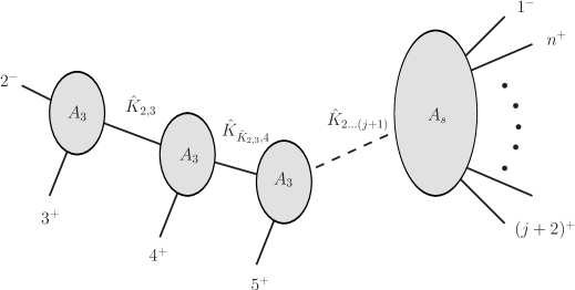
Our tactic to solve eq. (5) for $R_{n}(1,2)$ is to insert the left-hand side of eq. (5) into the right-hand side of eq. (5) repeatedly. At each insertion we find that our desired amplitude $R(1,2)$ appears on the right-hand side with one fewer positive-helicity leg, and multiplied by one more three-point gluon vertex and propagator, $A^{{\rm tree}}_{3}/K^{2}$. This ‘unwinding’ of the amplitude continues until we have reduced the right-hand side of $R_{n}$ (eq. (5)) down to, in this case, $R_{4}=0$ and a sum of terms that contain only known quantities (e.g. $A_{s}$ and overlap terms $O$) multiplied by strings of $A^{{\rm tree}}_{3}$ vertices, a contributing example is shown in figure 2.

Figure 2: A contribution to the “unwinding”, the string of $A_{3}$ terms simplifies to $A_{j+1}(1^{-},2^{-},3^{+},\ldots,(j+1)^{+})/\langle 1\hat{K}_{2\ldots{j+1}}\rangle^{2}$.

At each step of the unwinding we must choose new shifted momenta. We always choose to shift the two negative-helicity legs of $R$. For example, after the first step we choose ${[\hat{1},\hat{K}_{2,3}\rangle}$ as the shifted legs. Similarly, when we perform a second insertion, of $R_{n-2}$, we choose the intermediate $\hat{K}$ momentum leg of the last shift and the previously shifted $\hat{1}$ leg.

After this “unwinding” each resulting term can be expressed schematically in the form

$$\Biggl{(}\prod_{r=2}^{j+1}\frac{iA^{{\rm tree}}_{3r}}{K^{2}_{r}}\Biggr{)}A_{s}(1^{-},\hat{K}^{-},(j+2)^{+},\ldots,n^{+})\,.$$ (6)

The product of three point gluon vertices contained inside the brackets is equivalent to simply a tree amplitude divided by $\vphantom{\hat{K}}\langle\smash{1}\,\smash{\hat{K}_{2\ldots(j+1)}}\rangle^{2}$. Hence the recursion is solved as eq. (6) is written entirely in terms of objects we know

$$\frac{iA^{{\rm tree}}_{j+1}(1^{-},2^{-},\ldots,(j+1)^{+})}{\vphantom{\hat{K}}\langle\smash{1}\,\smash{\hat{K}_{2\ldots(j+1)}}\rangle^{2}}A_{s}(1^{-},\hat{K}_{2\ldots(j+1)}^{-},(j+2)^{+},\ldots,n^{+})\,.$$

The complete unrenormalised scalar loop contribution is then given by

$$A^{\textrm{scalar}}_{n}=c_{\Gamma}\bigl{[}\hat{C}_{n}+R^{D}_{n}\bigr{]}+\frac{1}{3}A_{n}^{{\cal N}=1{\rm\ chiral}}+c_{\Gamma}\frac{2}{9}A_{n}^{\rm tree}\,,$$ (7)

as in this case $\textrm{Inf}\;A_{n}=0$. The cut-completed contribution, $\hat{C}_{n}$, previously calculated from unitarity techniques is given in Ref. [15] and

$$R^{D}_{n}(1,2) = \sum_{m=2}^{n-3}\frac{iA^{{\rm tree}}_{m}(1^{-},2^{-},\ldots,m^{+})}{\langle 1\,\hat{K}_{2\ldots m}\rangle^{2}}\Big{(}A_{s}(1^{-},\hat{K}_{2\ldots m}^{-},(m+1)^{+},\ldots,n^{+})$$ (8)

$$\hskip 56.9055pt\hbox{}+O_{n-m+2}(1^{-},\hat{K}_{2\ldots m}^{-},(m+1)^{+},\ldots,n^{+})$$

$$\hskip 56.9055pt\hbox{}+\widehat{CR}_{n-m+2}(1^{-},\hat{K}_{2\ldots m}^{-},(m+1)^{+},\ldots,n^{+})\Big{)}\,,$$

were in the recursion for $R_{n}^{D}$ both the overlap, $O_{n}$ pieces, and the cut-completion $\widehat{CR}_{n}$ terms are included. Inserting the known forms of these terms into eq. (8) produces the result given in Ref. [15].

This “unwinding” technique also extends to other processes, so far this has included all-multiplicity massive scalar trees [10] and the all-multiplicity MHV one-loop gluonic QCD amplitude [14]. Hence the unitarity bootstrap approach provides a bright new outlook on the calculation of previously difficult to compute loop process needed to fully exploit the promise of the LHC.

References

- [1] A. Denner, S. Dittmaier, M. Roth and L. H. Wieders, Phys. Lett. B612:223 (2005) [hep-ph/0502063]; Nucl. Phys. B724:247 (2005) [hep-ph/0505042]; W. T. Giele and E. W. N. Glover, JHEP 0404:029 (2004) [hep-ph/0402152]; R. K. Ellis, W. T. Giele and G. Zanderighi, JHEP 0605:027 (2006) [hep-ph/0602185]; T. Binoth, G. Heinrich and N. Kauer, Nucl. Phys. B654:277 (2003) [hep-ph/0210023]; M. Kramer and D. E. Soper, Phys. Rev. D66:054017 (2002) [hep-ph/0204113]; T. Binoth, J. P. Guillet, G. Heinrich, E. Pilon and C. Schubert, JHEP 0510:015 (2005) [hep-ph/0504267].
- [2] Z. Bern, L. J. Dixon, D. C. Dunbar and D. A. Kosower, Nucl. Phys. B425:217 (1994) [hep-ph/9403226]; Z. Bern, L. J. Dixon and D. A. Kosower, Ann. Rev. Nucl. Part. Sci. 46:109 (1996) [hep-ph/9602280]; Z. Bern, L. J. Dixon and D. A. Kosower, Nucl. Phys. Proc. Suppl. 51C:243 (1996) [hep-ph/9606378]; Z. Bern, L. J. Dixon and D. A. Kosower, JHEP 0001:027 (2000) [hep-ph/0001001]; Z. Bern, L. J. Dixon and D. A. Kosower, Nucl. Phys. B513:3 (1998) [hep-ph/9708239]; Z. Bern, L. J. Dixon and D. A. Kosower, JHEP 0408:012 (2004) [hep-ph/0404293].
- [3] Z. Bern, L. J. Dixon, D. C. Dunbar and D. A. Kosower, Nucl. Phys. B435:59 (1995) [hep-ph/9409265].
- [4] Z. Bern and A. G. Morgan, Nucl. Phys. B467:479 (1996) [hep-ph/9511336].
- [5] Z. Bern, L. J. Dixon and D. A. Kosower, Nucl. Phys. B513:3 (1998) [hep-ph/9708239].
- [6] R. Britto, F. Cachazo and B. Feng, Nucl. Phys. B725:275 (2005) [hep-th/0412103]; A. Brandhuber, S. McNamara, B. Spence and G. Travaglini, JHEP 0510:011 (2005) [hep-th/0506068]; Z. Bern, L. J. Dixon and D. A. Kosower, JHEP 0408:012 (2004) [hep-ph/0404293]; Z. Bern, V. Del Duca, L. J. Dixon and D. A. Kosower, Phys. Rev. D71:045006 (2005) [hep-th/0410224]; R. Britto, E. Buchbinder, F. Cachazo and B. Feng, Phys. Rev. D72:065012 (2005) [hep-ph/0503132]; R. Britto, B. Feng and P. Mastrolia, Phys. Rev. D73:105004 (2006) [hep-ph/0602178].
- [7] Z. Bern, L. J. Dixon, D. C. Dunbar and D. A. Kosower, Phys. Lett. B394:105 (1997) [hep-th/9611127].
- [8] Z. Bern, L. J. Dixon and D. A. Kosower, JHEP 0001:027 (2000) [hep-ph/0001001]; Z. Bern, L. J. Dixon and D. A. Kosower, JHEP 0408:012 (2004) [hep-ph/0404293]; D. A. Kosower and P. Uwer, Nucl. Phys. B563: 477 (1999) [hep-ph/9903515]; Z. Bern, A. De Freitas and L. J. Dixon, JHEP 0203:018 (2002) [hep-ph/0201161]; A. Brandhuber, S. McNamara, B. Spence and G. Travaglini, JHEP 0510:011 (2005) [hep-th/0506068].
- [9] S. D. Badger, E. W. N. Glover, V. V. Khoze and P. Svrček, JHEP 0507:025 (2005) [hep-th/0504159]; S. D. Badger, E. W. N. Glover and V. V. Khoze, JHEP 0601:066 (2006) [hep-th/0507161]; C. Schwinn and S. Weinzierl, JHEP 0603:030 (2006) [hep-th/0602012]; P. Ferrario, G. Rodrigo and P. Talavera, Phys. Rev. Lett. 96:182001 (2006) [hep-th/0602043].
- [10] D. Forde and D. A. Kosower, Phys. Rev. D73:065007 (2006) [hep-th/0507292].
- [11] R. Britto, F. Cachazo and B. Feng, Nucl. Phys. B715:499 (2005) [hep-th/0412308]; R. Britto, F. Cachazo, B. Feng and E. Witten, Phys. Rev. Lett. 94:181602 (2005) [hep-th/0501052].
- [12] M.-X. Luo and C.-K. Wen, JHEP 0503:004 (2005) [hep-th/0501121]; Phys. Rev. D71:091501 (2005) [hep-th/0502009]; R. Britto, B. Feng, R. Roiban, M. Spradlin and A. Volovich, Phys. Rev. D71:105017 (2005) [hep-th/0503198]; K. J. Ozeren and W. J. Stirling, JHEP 0511:016 (2005) [hep-th/0509063]; M. Dinsdale, M. Ternick and S. Weinzierl, JHEP 0603:056 (2006) [hep-ph/0602204]; D. de Florian and J. Zurita, JHEP 0605:073 (2006) [hep-ph/0605291].
- [13] Z. Bern, L. J. Dixon and D. A. Kosower, Phys. Rev. D71:105013 (2005) [hep-th/0501240]; Z. Bern, L. J. Dixon and D. A. Kosower, Phys. Rev. D72:125003 (2005) [hep-ph/0505055].
- [14] Z. Bern, L. J. Dixon and D. A. Kosower, Phys. Rev. D73:065013 (2006) [hep-ph/0507005]; C. F. Berger, Z. Bern, L. J. Dixon, D. Forde and D. A. Kosower, arXiv:hep-ph/0604195; C. F. Berger, Z. Bern, L. J. Dixon, D. Forde and D. A. Kosower, arXiv:hep-ph/0607014.
- [15] D. Forde and D. A. Kosower, Phys. Rev. D 73, 061701 (2006) [arXiv:hep-ph/0509358].
- [16] M. L. Mangano and S. J. Parke, Phys. Rept. 200:301 (1991); L. J. Dixon, in QCD & Beyond: Proceedings of TASI ’95, ed. D. E. Soper (World Scientific, 1996) [hep-ph/9601359]; Z. Bern and G. Chalmers, Nucl. Phys. B447:465 (1995) [hep-ph/9503236].
- [17] C. .F. Berger, arXiv:hep-ph/0608027.