Isolating Vector Boson Scattering at the LHC: gauge cancellations and the Equivalent Vector Boson Approximation vs complete calculations.

Abstract

We have studied the possibility of extracting the $W^{+}W^{-}\rightarrow W^{+}W^{-}$ signal using the process $us\rightarrow cdW^{+}W^{-}$ as a test case. We have investigated numerically the strong gauge cancellations between signal and irreducible background, analysing critically the reliability of the Equivalent Vector Boson Approximation which is commonly used to define the signal. Complete matrix elements are necessary to study Electro–Weak Symmetry Breaking effects at high $WW$ invariant mass.

I Introduction

The mechanism of Electro–Weak Symmetry Breaking (EWSB) will be one of the primary topics to be investigated at the LHC, both through direct searches for the Higgs boson and careful analysis of boson boson scattering processes. Detailed reviews and extensive bibliographies can be found in Refs.atl:99atl ; Assamagan:2004mu ; Djouadi:2005gi . The nature of the interaction between longitudinally polarized vector bosons and the Higgs mass, or possibly the absence of the Higgs particle, are strongly related: if a relatively light Higgs exists then the ${\mathrm{V}_{L}}$’s are weakly coupled, while they are strongly interacting if the Higgs mass is large or the Higgs is nonexistent Chanowitz:1998wi .

It should be noted that the Goldstone theorem and the Higgs mechanism do not require the existence of elementary scalars. It is conceiveable and widely discussed in the literature that bound states are responsible for EWSB.

At the LHC no beam of on shell EW vector bosons will be available. Incoming quarks will emit spacelike virtual bosons which will then scatter among themselves and finally decay. These processes have been scrutinized since a long time in order to uncover the details of the EWSB mechanism in this realistic setting Duncan:1985vj ; Dicus:1986jg ; Gunion:1986gm . Naively one expects that at large boson boson invariant masses the diagrams containing vector boson fusion subdiagrams should dominate the total cross section while the offshellness of the bosons initiating the scattering process should become less and less relevant. Together with the keen interest for Higgs production in vector boson fusion, this has lead to the development of the Equivalent Vector Boson Approximation (EVBA) Dawson:1984gx ; Kane:1984bb ; Lindfors:1985yp . The EVBA provides a particularly simple and appealing framework in which the cross section for the full process is approximated by the convolution of the cross section for the scattering of on shell vector bosons times appropriate distribution functions which can be interpreted as the probability of the initial state quarks to emit the EW bosons which then interact.

This approach relies on the neglect of all diagrams which do not include boson boson scattering subdiagrams and on a suitable on-shell projection for the scattering set of diagrams. Since the approximate boson boson interaction is expressed in terms of on shell particles it is straitforward to separate the different boson polarizations. It is well known that the set of scattering diagrams is not separately gauge invariant while both the on shell amplitude and the distribution functions which appear in the EVBA are gauge independent.

In Kleiss:1986xp it has been shown that when vector bosons are allowed to be off mass shell in boson boson scattering, the amplitude grows faster with energy compared with the amplitude for on shell vectors. Subsequently, it has been pointed out in Kunszt:1987tk that the problem of bad high energy behaviour of $WW$ scattering diagrams can be avoided by the use of the Axial gauge. Recently $WZ$ production at hadron collider Accomando:2006iz has been analyzed in Axial gauge with very encouraging results. It should be noted that the results in Kunszt:1987tk have been obtained under the assumption that the transverse momenta of the produced $W$’s are of the order of the Higgs mass and that each are much larger than the $W$ mass. It is therefore not obvious to what degree the conclusions of Ref.Kunszt:1987tk can be applied in the LHC environment, particularly for light Higgs masses as preferred by global SM fits.

The EVBA has some undesirable features: a number of unphysical cuts need to be introduced to tame the singularities generated by the onshell projection, which are absent from the exact amplitude. In the literature, a number of comparisons of exact and EVBA calculations have appeared with conflicting results Cahn:1984tx ; Willenbrock:1986cr ; Gunion:1986gm

For these reasons in the present paper we have critically examined the role of gauge invariance in ${\mathrm{V}}{\mathrm{V}}$-fusion processes and the reliability of the EVBA in describing them. We would like to determine regions in phase space, at least in a suitable gauge, which are dominated by the scattering set of diagrams.

If this was the case then it would be possible employ this set of diagrams to define a “signal”, that is a pseudovariable which could be used to compare the results from the different collaborations. The signal is not necessarily directly observable but it should be possible to relate it via Monte Carlo to measurable quantities. If such a definition is to be useful it must correspond as closely as possible to the process which needs to be studied and the Monte Carlo corrections must be small. If instead, as we are led to believe by the results shown in the following, the VV scattering diagrams do not constitute the dominant contribution in any gauge or phase space region, there is no substitute to the complete amplitude for studying boson fusion processes at the LHC. We cannot claim to have examined all possible gauge scheme, however we have studied the most commonly used $\xi$–type gauges and the implementation of the Axial gauge proposed in Kunszt:1987tk . The results obtained with the full amplitude show that the mechanism of EWSB can indeed be investigated even without separating out the scattering set of diagrams.

II VV -Scattering and gauge invariance

In order to study the implications of gauge invariance in ${\mathrm{V}}{\mathrm{V}}$-fusion processes we have concentrated on the specific process $us\rightarrow cdW^{+}W^{-}$ in proton proton collisions at the LHC. The corresponding Feynman diagrams can be classified in two different sets (Fig. 1), the boson boson fusion one (Fig. 1a) and all the rest (Fig. 1b) in which at least one final W is emitted by a fermion line. The two sets are not separately gauge invariant. We have started our analysis from the contribution of the boson boson fusion diagrams and their interference with the remaining ones. We have considered the Unitary, Feynman and Landau gauge. Among these, we find that the Feynman gauge is the one which minimizes the cancellations between set (a) of Fig. 1 and the non scattering diagrams. We have also performed the calculation in the Axial gauge $n_{\mu}A^{\mu}=0$ within the scheme proposed in Ref.Kunszt:1987tk . In Appendix.A we have collected the main corresponding Feynman rules. We have tried different $n_{\mu}$ gauge vectors and we find that the choice $n_{\mu}=(1,0,0,1)$ (The incoming protons propagate along the z axis) is the best one. For brevity we will refer to this framework as Axial gauge in the following. We present results for the Unitary, Feynman and Axial gauge, showing the contribution of all diagrams ($all$), of the $WW$ scattering diagrams ($WW$) together with their ratio $WW/all$. When this ratio is significantly greater than one the contribution of non scattering diagrams is of the same order as the contribution of the $WW$ scattering ones and important cancellations take place between the two sets.

In Tab. 1 the total cross sections and their ratios are computed in the limit of infinite Higgs mass. This limit will also be referred to in the following as noHiggs case. We find that the Axial gauge is the one in which the interferences are least severe with a ratio of about 2, while the ratios for the Unitary and Feynman gauge are 358 and 13 respectively. The inclusion of a light Higgs ($M_{h}$=200 GeV) does not improve matters: on the contrary the ratios become even larger as shown in Tab. 2 for $M_{h}$=200 GeV, doubling for the Unitary and Feynman gauge

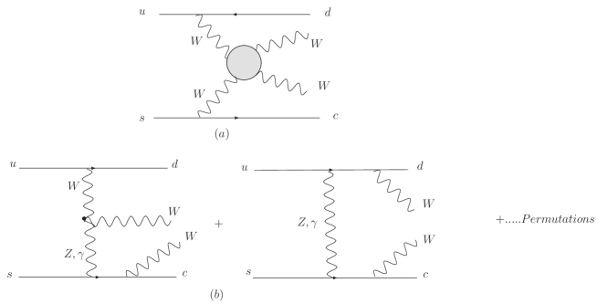
Figure 1: Main diagram topologies for the process $us\rightarrow cdW^{+}W^{-}$

	$\sigma(pb)$ All diagrams	$\sigma(pb)$ $WW$ diagrams	ratio $WW/all$
Unitary gauge	1.86 10-2	6.67	358
Feynman gauge	1.86 10-2	0.245	13
Axial gauge	1.86 10-2	3.71 10-2	2

Table 1: $WW$ diagrams and complete set of diagrams cross sections and their ratios computed in different gauges without Higgs contribution. We have used the CTEQ5 Pdf set with scale $M_{W}$

	$\sigma(pb)$ All diagrams	$\sigma(pb)$ $WW$ diagrams	ratio $WW/all$
Unitary gauge	8.50 10-3	6.5	765
Feynman gauge	8.50 10-3	0.221	26
Axial gauge	8.50 10-3	2.0 10-2	2.3

Table 2: $WW$ diagrams and complete set of diagrams cross sections and their ratios computed in different gauges with a $M_{h}$ =200 GeV Higgs and $M(WW)>$ 300 GeV .

The comparison of total cross sections is only a preliminary step. It provides the general behavior but it cannot give informations on the different regions of phase space. For this reason we have evaluated the distribution of different kinematical variables with the goal of finding regions where the interferences are not important. If such regions exist it will be possible to define a set of cuts which allow the extraction of the $WW$ scattering amplitude. Fig. 2 shows the distributions of the diboson invariant mass for the complete set of diagrams and for the $WW$ diagrams only together with the ratio $(d\sigma(WW)/dM)/(d\sigma(All)/dM)$ . We have chosen the vector boson pair invariant mass distribution as a prototype but the same conclusions are reached with all other variables. The results of Fig. 2 have been obtained for a very large Higgs mass but the general behaviour is not modified by the inclusion of a light Higgs. The distribution obtained with the full set of diagrams and with the $WW$ fusion set only are quite different in Unitary and Feynman gauge. The ratio is also large over the whole interval and especially in the region of high invariant mass which is the most important one for EWSB studies. Again the Axial gauge gives the best result, with distributions which have the same general shape in the two cases. The ratio in this gauge remains however greater than 2, apart from a very small region at low invariant mass.

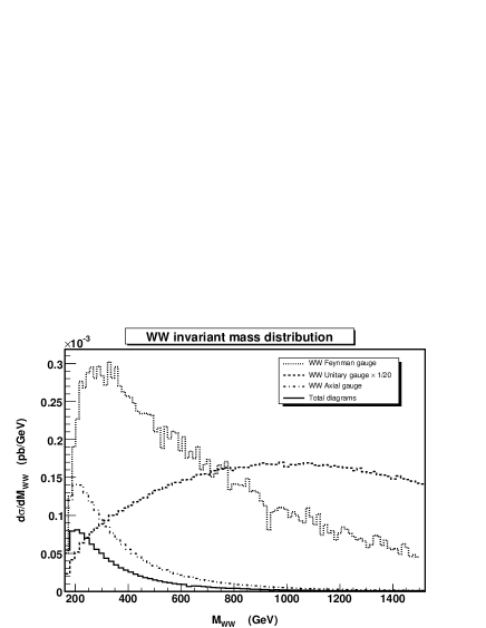
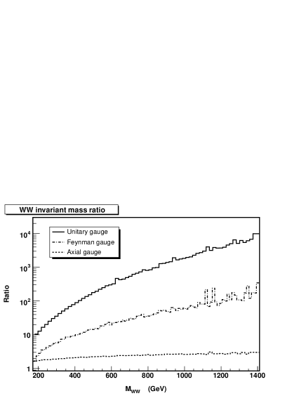
Figure 2: Distribution of $d\sigma/dM_{WW}$ for the process $PP\rightarrow us\rightarrow cdW^{+}W^{-}$ for All diagrams, $WW$ diagrams and their ratio in Unitary, Feynman and Axial gauge in the infinite Higgs mass limit. The Unitary gauge data in the left hand plot have been divided by 20 for better presentation.

We have completed our study by analyzing bi-dimensional distributions of several pairs of kinematical variables. These double distributions allow us to analyze in particular the situation where the two incoming bosons have small virtualities ($t_{1,2}\rightarrow 0$). In this region the $WW$ scattering diagrams are expected to dominate. The same behaviour found previously is observed: the effect of the interferences is much more relevant in Unitary gauge with respect to the others. In general the $WW$ fusion subset has a different behavior compared with the complete calculation. In Fig. 3 we report $d\sigma/dt_{1}dt_{2}$ in the Axial gauge where $t_{1,2}=\sqrt{-(p_{u,s}-p_{d,c})^{2}}$ are the square root of the absolute value of the invariant masses of the incoming off shell W’s. The corresponding ratio distributions (plots (c) (d)) show that even in the limited region $0<t_{1,2}<250$ GeV, the $WW$ contribution alone does not provide a realistic description of the complete set of diagrams. Even in Axial gauge significant cancellations take place. The ratio is highly asymmetric in the $t_{1}-t_{2}$ plane, reflecting its sensitivity to the choice of the Axial gauge axis (Recall that in this case the gauge vector is along the $z$–axis) and $WW$ scattering diagrams alone provide only a very rough estimate of the cross section. It is however possible to find regions, typically for $t_{1,2}>200$ GeV where the cross section is greatly reduced, where the ratio of the two results is around one. For comparison we also show the distributions obtained from the $WW$ fusion subset in the Unitary (e) and Feynman (f) gauge whose shape, not to mention the normalization, is completely different from the results obtained from the full amplitude.

From this sample of results one can conclude that the $WW$ scattering diagrams do not constitute the dominant contribution in any phase space region for the gauges we have examined. For the Axial gauge, which in various cases shows ratios of order 2, we remark that these have been obtained only with a particular time like gauge vector $n_{\mu}=(1,0,0,1)$. For any other space-like $n_{\mu}$, the interferences are so important that even the numerical integration becomes difficult for the $WW$ diagrams set whereas no problem occurs for the full set of diagrams. So we did not succeed in finding a gauge vector of the type suggested in Kunszt:1987tk for which the cancellations are negligible. Even with our best choice of $n_{\mu}$ the distributions of the different kinematical variables show the presence of large interferences between the two subset of diagrams over most of phase space, indicating that the $WW$ diagrams are not dominating. As a consequence a question mark is put on the possibility to isolate the $WW$ scattering contribution by restricting the calculations to the corresponding diagrams. The reliability of approximation methods based on such an approach becomes then suspicious. For this reason we have completed our analysis by studying the Effective Vector Boson Approximation applied to our prototype process.

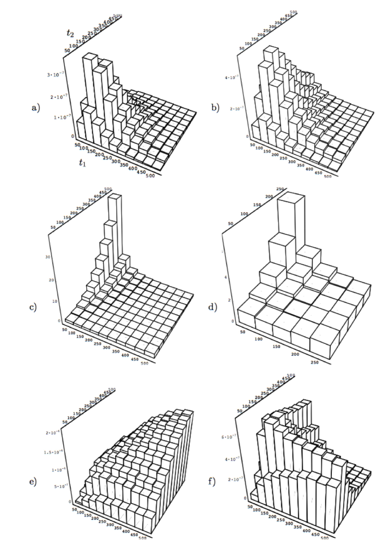
Figure 3: Double differential distributions of $d\sigma/dt_{1}dt_{2}$ $(pb/GeV^{2})$ with $t_{1,2}=\sqrt{-(p_{u,s}-p_{d,c})^{2}}$ for the process $PP\rightarrow us\rightarrow dcW^{+}W^{-}$ , using All diagrams (a) or only the $WW$ fusion subset in Axial gauge (b). The two plots in the central row represent the ratio $WW/all$ in the Axial gauge as a function of $t_{1},t_{2}$ for the total region (c) and for small $t$’s (d). For comparison we also show the distributions of the $WW$ fusion subset in the Unitary (e) and Feynman (f) gauge. All invariants are in GeV.

III The Effective Vector Boson Approximation

The Effective Photon Approximation known also as Weizsäcker-Williams approximation vonWeizsacker:1934sx ; Williams:1934ad has proved to be a useful tool in the study of photon-photon processes at $e^{+}e^{-}$ colliders. Encouraged by this success the approach has been extended to processes involving massive vector bosons Dawson:1984gx ; Kane:1984bb ; Lindfors:1985yp under the name of Effective Vector Boson Approximation. The EVBA has been first applied at hadron colliders in connection with Higgs production $pp\rightarrow H+X$ Cahn:1983ip and subsequently to vector boson processes of the type $pp\rightarrow(H\rightarrow V_{3}V_{4})+X\rightarrow V_{3}V_{4}+X$ Gunion:1986gm ; Chanowitz:1984ne in order to obtain EVBA predictions for the production of a vector boson pair not necessarily near the Higgs resonance and to study the strongly interacting scenario.

In analogy to the QED case, the application of EVBA to these processes consists in:

1. Restricting the computation to the vector boson scattering diagrams neglecting diagrams of bremsstrahlung type.

2. Projecting on-shell the momenta of the vector bosons which take part to the scattering: $q^{2}_{1,2}=M^{2}_{V_{1,2}}$. Here it is important to notice that contrary to the $\gamma\gamma$ processes where the photon momentum can reach the on shell value $q^{2}_{1,2}=0$, for the massive vector bosons the onshell point $q^{2}_{1,2}=M^{2}_{V_{1,2}}$ is outside the accessible phase space region $q^{2}_{1,2}\leq 0$.

3. Approximating the total cross section of the process $f_{1}f_{2}\rightarrow f_{3}f_{4}V_{3}V_{4}$ as the convolution of the vector boson luminosities $\mathcal{L}^{V_{1}V_{2}}_{Pol_{1}Pol_{2}}(x)$ with the on shell vector boson scattering cross section:

$$\sigma(f_{1}f_{2}\rightarrow f_{3}f_{4}V_{3}V_{4})=\int\sum_{V_{1},V_{2}}\sum_{Pol_{1}Pol_{2}}{\mathcal{L}^{V_{1}V_{2}}_{Pol_{1}Pol_{2}}(x)}\sigma^{on}_{pol}(V_{1}V_{2}\rightarrow V_{3}V_{4},xs_{qq})dx$$ (1)

Here $x=M(V_{1}V_{2})^{2}/s_{qq}$, while $M(V_{1}V_{2})$ is the vector boson pair invariant mass and $s_{qq}$ is the partonic center of mass energy.

It is clear that this approximation provides a simplification from the computational point of view and can exploit the properties of on shell boson boson scattering. In first applications of EVBA to vector boson scattering further approximations have been adopted. The zero angle scattering approximation has been used for the process $V_{1}V_{2}\rightarrow V_{3}V_{4}$ so the transverse momentum of the incoming bosons has been neglected. The zero mass limit for the vector boson mass $M_{V}\rightarrow 0$ has also been considered in the computation of the luminosity. In this early application of EVBA only the contribution from longitudinal modes was considered while the contribution from transverse states was neglected. The EVBA results depended strongly on the details of the approximations made. The EVBA generally overestimated the complete perturbative calculation, in some cases by a factor 3 Godbole:1987iy . Progressively, more refined and rigorous formulations of EVBA have been proposed, avoiding as much as possible the mentioned approximations, until a formulation where no kinematical approximations are taken and all vector boson polarization states as well as their interferences are taken into account Kuss:1995yv . Inspired by the strategy of Kuss:1995yv , we have further improved the EVBA. We have used an approach where not only all kinematic approximations are avoided but also the luminosity computation is not needed. This allows in particular to keep all final particle properties (momenta, angles…) as they would be in an exact calculation contrary to the traditional approach where a pre-integration is performed to obtain the vector boson luminosities.

IV EVBA application to the $PP\rightarrow us\rightarrow dcW^{+}W^{-}$ process

In Kuss:1995yv a precise formulation of EVBA has been developed. It is based on a factorization technique for analyzing Feynman diagrams which leads to exact probability distribution functions for the vector bosons Johnson:1987tj . This improved formulation does not invoke any kinematical approximation such as those mentioned in the previous paragraph. The only approximation concerns the on shell continuation of the vector boson scattering cross section. Using this factorization technique and the relation between the polarization vectors and the vector boson propagator in Unitary gauge, the matrix element for any process of the kind $f_{1}f_{2}\rightarrow f_{3}f_{4}+Y$, where $Y$ is produced by vector boson fusion, can be written as:

$$M=e^{2}\sum_{m,n=-1}^{1}(-1)^{m+n}\frac{j_{1}(p_{1},p_{3}).\epsilon^{*}_{1}(m)}{q_{1}^{2}-M_{V_{1}}^{2}}\times\frac{j_{2}(p_{2},p_{4}).\epsilon^{*}_{2}(n)}{q_{2}^{2}-M_{V_{2}}^{2}}\times M(m,n)$$ (2)

$q_{1,2}$ are the momenta of the initial vector bosons, $\epsilon_{j}(m)$ are their polarization vectors corresponding to the different helicity states $m=0,\pm 1$. We have used the same expressions, conventions and frame to define them as given in Kuss:1995yv . They are normalized according to :

$$\epsilon_{j}(m)\cdot\epsilon_{j}^{*}(m^{\prime})=\delta_{m,m^{\prime}}(-1)^{m}$$ (3)

and satisfy the completeness relation:

$$\sum_{m=-1,0,1}\epsilon_{j}^{\mu}(m)\epsilon_{j}^{*\nu}(m)=-g^{\mu\nu}+\frac{q^{\mu}q^{\nu}}{M_{V_{j}}^{2}}$$ (4)

$j_{1,2}$ are the quark currents and $M(m,n)$ the off shell scattering amplitude of the vector boson subprocess $V_{1}V_{2}\rightarrow V_{3}V_{4}$:

$$M(m,n)=\sum_{\mu\nu\alpha\beta}\epsilon_{1}^{\mu}(m)\epsilon_{2}^{\nu}(n)T_{\mu\nu\alpha\beta}\epsilon_{3}^{*\alpha}\epsilon_{4}^{*\beta}$$ (5)

Usually an integration is performed over all the integration variables which are not concerned with the vector boson scattering subprocess as a first step to compute the vector boson luminosities. Denoting these variables by $\{\phi\}$, one can write the total cross section expression as:

$$\sigma_{tot}=\int g(q_{1}^{2},q_{2}^{2},x,\phi)d\phi\>\sigma^{VV}_{off}(W^{2},q_{1}^{2},q_{2}^{2})dq_{1}^{2}dq_{2}^{2}dx$$ (6)

$g(q_{1}^{2},q_{2}^{2},x,\phi)$ represents all terms which are independent of the vector boson scattering subprocess. Here $x=\frac{W^{2}}{s_{qq}}$, where $W^{2}=(q_{1}+q_{2})^{2}$ is the diboson invariant mass squared.

$$\sigma^{VV}_{off}(W^{2},q_{1}^{2},q_{2}^{2})\sim\int\sum_{m,n,m^{\prime},n^{\prime}}M(m,n)M^{*}(m^{\prime},n^{\prime})dp_{V}$$ (7)

is the off shell $VV\rightarrow VV$ cross section and $dp_{V}$ the final state vector boson phase space element. The next step is the extrapolation to on shell masses. In Kuss:1995yv it is achieved by simple proportionality factors between the off shell and on shell cross sections:

$$\sigma^{off}_{pol}(W^{2},q_{1}^{2},q_{2}^{2})=f_{pol}(W^{2},q_{1}^{2},q_{2}^{2})\sigma^{on}_{pol}(W^{2},M_{V_{1}}^{2},M_{V_{2}}^{2})$$ (8)

the subscript $pol$ refers to the different vector boson polarization states, and $M_{V_{1}}$, $M_{V_{2}}$ the masses of the vector bosons initiating the scattering process. While we refer to Kuss:1995yv for the details, we reproduce here the form factors $f_{pol}$ expression according to the different polarization configurations:

$$f_{TT}=1\>;\>f_{LL}=(\frac{M_{V_{1}}^{2}}{-q_{1}^{2}})(\frac{M^{2}_{V_{2}}}{-q_{2}^{2}})$$ (9)

$$f_{LT}=(\frac{M_{V_{1}}^{2}}{-q_{1}^{2}})\>;\>f_{TL}=(\frac{M_{V_{2}}^{2}}{-q_{2}^{2}})$$ (10)

$$f_{TLTL}=(\frac{M_{V_{1}}}{\sqrt{-q_{1}^{2}}})(\frac{M_{V_{2}}}{\sqrt{-q_{2}^{2}}})$$ (11)

Finally one can write the cross section expression in the EVBA approximation as:

$$\sigma^{EVBA}_{tot}=\int g(q_{1}^{2},q_{2}^{2},x,\phi)d\phi dq_{1}^{2}dq^{2}_{2}\sum_{Pol_{1}Pol_{2}}f_{pol}\sigma^{on}_{pol}dx$$ (12)

By comparison with eq.(1) the luminosity can be expressed as:

$${\mathcal{L}^{WW}_{Pol_{1}Pol_{2}}(x)}=\int g(q_{1}^{2},q_{2}^{2},x,\phi)f_{pol}d\phi dq_{1}^{2}dq^{2}_{2}$$ (13)

In our implementation we have used the same assumptions but we have performed the onshell extrapolation at the matrix element level. This allows to keep all the terms $M(m,n)M^{*}(m^{\prime},n^{\prime})$ ($m\neq m^{\prime},n\neq n^{\prime}$) in the total amplitude square expression. The offshell vector boson scattering matrix element $M(m,n)$ in (2) and (5) is expressed in terms of the corresponding on shell matrix elements and the polarization factors (9) as

$$M(m,n)=\sqrt{f_{mn}}M^{on}(m,n)\>\>\>\>\>(m,n=L,T).$$ (14)

Moreover we have not employed any luminosity function but we have used the diagrammatical expression of the fermion lines, evaluating them for each kinematical configuration and polarization.

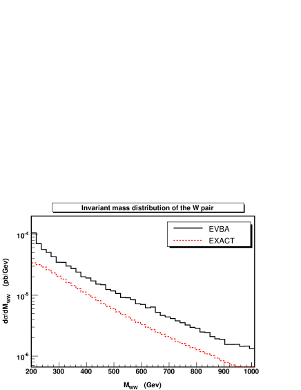
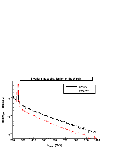
Figure 4: $WW$ invariant mass distribution $M(WW)$ for the process $us\rightarrow dcW^{+}W^{-}$ with EVBA (black solid curve) and with exact complete computation (red dashed curve) for the Infinite Higgs mass case (left) and $M_{h}$=250 GeV (right) at the LHC.

V Comparison between EVBA and exact results

We have computed the total cross section and the distribution of the vector boson pair invariant mass $M(WW)$ with an exact calculation and in EVBA for the process $PP\rightarrow us\rightarrow cdW^{+}W^{-}$ at the LHC. Cuts are necessary in EVBA to avoid the photon $t$ channel propagator pole and the form factor (9) ($q_{1}^{2}\rightarrow 0,q_{2}^{2}\rightarrow 0$) singularities. We have restricted the CM scattering angle of the W’s and the laboratory frame polar angle of the c and d quarks in order to deal with photon and form factor singularities respectively. For comparison purpose, the same cuts have also been applied in the exact calculation even though no singularity appears in this case. Unless otherwise noted, we have used a cut of 10 degrees for all three angles.

For the total cross section in the noHiggs case we obtain 0.63 10^-2 $pb$ with an exact calculation and 1.36 10^-2 $pb$ in EVBA. For $M_{h}$=250 GeV we obtain 1.32 10^-2 $pb$ and 1.64 10^-2 $pb$ respectively. The corresponding distributions of the $WW$ invariant mass is shown fig. 4. The ratio of the two results is . The EVBA overestimates the exact calculation by a factor of about two, which is almost insensitive to $M(WW)$, with the exception of the Higgs peak region at $M_{h}$= 250 GeV where the exact result is larger than the EVBA one.

We have checked our implementation of the EVBA against the one used in PYTHIA for the scattering of longitudinally polarized $W$’s. The two results are only in qualitative agreement as expected both for the total cross section and for distributions.

$M_{h}$	EVBA $(pb)$	EXACT $(pb)$	Ratio
$\infty$	3.90 10-2	1.78 10-2	2.17
130 GeV	3.94 10-2	1.71 10-2	2.3
250 GeV	4.61 10-2	4.09 10-2	1.12
500 GeV	4.42 10-2	2.5 10-2	1.77

Table 3: Total cross sections computed with EVBA and exact computation and their ratio for the process $us\rightarrow cdW^{+}W^{-}$ at fixed CM energy $\sqrt{s}=1$ TeV.

$\theta_{cut}$	EVBA $(pb)$	EXACT $(pb)$	Ratio
$10^{\circ}$	4.42 10-2	2.5 10-2	1.77
$30^{\circ}$	1.33 10-2	2.06 10-2	0.64
$60^{\circ}$	6.06 10-3	1.28 10-2	0.47

Table 4: Total cross section in EVBA and exact computation and their ratio for different angular cuts. The CM energy is $\sqrt{s}=1$ TeV and the Higgs mass $M_{h}$=500 GeV.

In previous works Gunion:1986gm the same partonic process $us\rightarrow cdW^{+}W^{-}$ has been used for EVBA $vs$ exact comparisons at fixed energy. For this reason we have tried to reproduce the results of Gunion:1986gm , using as closely as possible the same cuts and parameters. On one side this represented a test of our implementation of EVBA and on the other side it allowed us to determine whether the EVBA results are improved by this new and more rigorous formulation. We have computed the total cross section at a fixed center of mass energy of 1 TeV in the limit of infinite Higgs mass and with Higgs masses $M_{h}$=130, 250, 500 GeV. In Tab. 3 the cross sections and corresponding ratio are reported. We have also compared a number of distributions obtained with the two versions of EVBA and with the exact calculation. Our more sophisticated implementation doe not appear to improve substantially the agreement with the exact results.

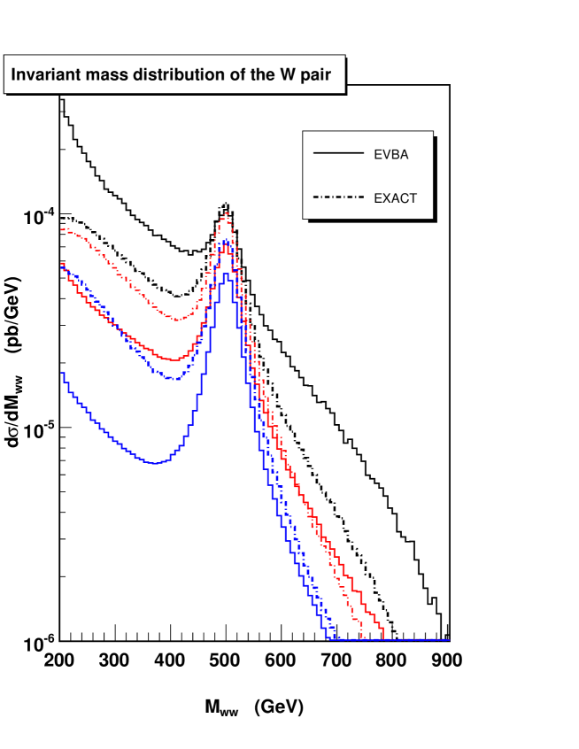
Figure 5: The $WW$ invariant mass distribution with different $\theta$-cut with EVBA (solid curves) and with the exact calculation (dashed curves). From top to bottom $\theta_{c}=10^{\circ}$ (black), $30^{\circ}$ (red), $60^{\circ}$ (blue). The CM energy is $\sqrt{s}=1$ TeV and $M_{h}$=500 GeV

Finally, we have analyzed the sensitivity of the results to the angular cut in the $M_{h}$=500 GeV Higgs case. The total cross section for $\theta_{cut}=\ 10^{\circ},\ 30^{\circ},\ 60^{\circ}$ are presented in Tab. 4 which shows that the EVBA is more sensitive to the angular cut than the exact computation. The corresponding $M(WW)$ distribution is shown in fig 5. We see that the relationship between the exact and EVBA results depends quite appreciably on the angular cut. The EVBA overestimates the exact result at $\theta_{cut}=\ 10^{\circ}$ by about a factor of two outside the Higgs peak, while the two distributions are in fair agreement at the resonance. However the EVBA underestimates the correct result at $\theta_{cut}=\ 60^{\circ}$ over the whole mass range. The difference decreases from about a factor of two at small invariant masses to roughly 20% at masses larger than the Higgs mass. Therefore, while it appears quite possibile to find a set of cuts, at fixed energy and Higgs mass, for which the EVBA approximation reproduces well the exact result for the total cross section, in general it is extremely difficult to extract from the EVBA more than a very rough estimate of the actual behaviour of the Standard Model predictions for boson boson scattering.

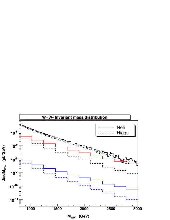
Figure 6: The $WW$ invariant mass distribution in $PP\rightarrow us\rightarrow cdW^{+}W^{-}$ at the LHC for the infinite Higgs mass case (solid curves) and for $M_{h}$=200 GeV (dashed curve). The two intermediate (red) curves have been obtained imposing the set of cuts described in the text. The two lowest (blue) curves refer to the process $PP\rightarrow us\rightarrow cd\mu^{-}\overline{\nu}_{\mu}e^{+}\nu_{e}$; in this case further acceptance cuts have been imposed on the charged leptons: $E_{l}>20$ GeV, $p_{T_{l}}>10$ GeV , $|\eta_{l}|<$ 3.

VI The large invariant mass region

The results presented in Sects. II, V lead to the conclusions that the boson boson subamplitude cannot reliably be extracted from the full $qq\rightarrow qqVV$ amplitude. However the full amplitude is sensitive to the details of the EWSB mechanism. If no light Higgs is present in the SM spectrum, some hitherto unknown mechanism must intervene to enforce unitarity of the S-Matrix which embodies the conservation of total probability. The infinite Higgs mass limit violates perturbative unitarity in onshell boson boson scattering but on the other hand can be computed exactly, while the many available models for unitarizing the theory deal exclusively with on shell bosons and can only approximately be incorporated in a decription of $qq\rightarrow qqVV$ processes or in a six final state fermion framework, which has recently become available for the LHC Accomando:2005cc ; ballestrero:2006pn .

E(quarks)$>20$ GeV
${\mathrm{p}_{T}}$ (quarks,W)$>10$ GeV
$2<|\eta$(quark)$|<6.5$
$|\eta$(W)$|<3$

Table 5: Selection cuts applied in Fig. 6.

At the LHC the linear rise of the cross section at large boson boson invariant masses squared entailed by the leading behaviour of boson boson scattering in the SM with a very large Higgs mass will be overcome by the decrease of the parton luminosities at large $x$ and will be particularly challenging to detect. In the absence of a more reliable theory we have adopted the noHiggs model as a poor man substitute.

In Fig. 6 we show the large mass tail of the boson pair invariant mass distribution for the noHiggs case and for a Higgs mass of 200 GeV. In the absence of cuts the two results differ by about 20% over the full range. With appropriate cuts the difference between the two cases can be significantly increased. Applying the selection cuts in Tab. 5 we obtain the two intermediate, red curves in Fig. 6. The two lowest (blue) curves refer to the full process $PP\rightarrow us\rightarrow cd\mu^{-}\overline{\nu}_{\mu}e^{+}\nu_{e}$; in this case further acceptance cuts have been imposed on the charged leptons: $E_{l}>20$ GeV, $p_{T_{l}}>10$ GeV , $|\eta_{l}|<$ 3. We see that the separation between the two Higgs mass hypotheses persists also in this more realistic setting.

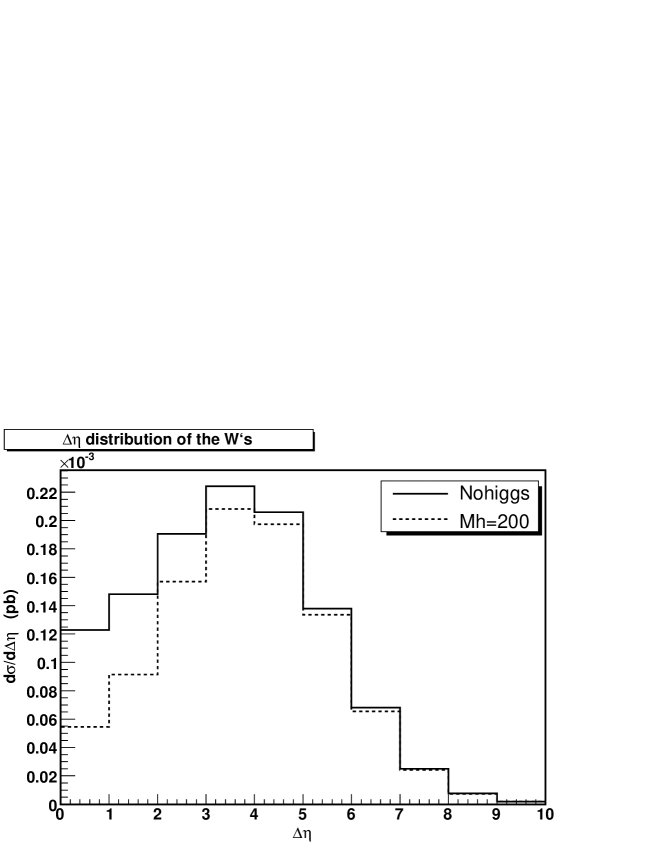
Figure 7: Distribution of the pseudorapidity difference between the two W’s for $us\rightarrow dcW^{+}W^{-}$ at the LHC for the Infinite Higgs mass case (solid curve) and $M_{h}$=200 GeV (dashed curve).

As an example of the different kinematical distributions in the two cases we show in Fig. 7 the absolute value of the difference between the pseudorapidities of the two $W$’s. It is interesting that the shape of the kinematical distributions, which are less sensitive to pdf uncertainties than their absolute normalization, behave differently when a light Higgs is present in the spectrum then when its mass is very large. For more details we refer to Accomando:2005hz ; Accomando:2006vj . We conclude that while it does not appear to be possible to study the contribution of the scattering diagrams in isolation from the remaining ones, the full amplitude, in the region of large $WW$ invariant masses at LHC energies, is sensitive to the presence of a light Higgs and therefore to the details of the mechanism of EWSB.

VII Conclusions

We have critically examined the role of gauge invariance in ${\mathrm{V}}{\mathrm{V}}$-fusion processes and the reliability of the EVBA in describing them in the Unitary, Feynman and Axial gauge. We have shown that the $WW$ scattering diagrams do not constitute the dominant contribution in any phase space region for the set of gauge fixing we have examined. The Axial gauge as proposed in Kunszt:1987tk results in less severe cancellations between the contribution of non scattering diagrams and the contribution of the $WW$ scattering ones but typically the two sets have comparable magnitude.

We have shown that EVBA results and their relationship to exact results depend quite sensitevely on the set of cuts which need to be applied in order to obtain a finite result. Therefore, it is extremely difficult to extract from the EVBA more than a very rough estimate of the actual behaviour of the Standard Model predictions for boson boson scattering.

We conclude that while it seems impossible to isolate the contribution of the scattering diagrams, the mechanism of EWSB can be investigated, using the full amplitude, by a careful analysis of the region of large $WW$ invariant masses at the LHC.

Appendix A Axial gauge

We report here for convenience the main formulae describing the Axial gauge formulation of Kunszt:1987tk to which we refer for a more detailed discussion.

Parametrizing the Higgs field as

$$\phi(x)=\left(\begin{array}[]{c}iw(x)\\ \sqrt{\frac{1}{2}}[v+h(x)+iz(x)]\end{array}\right)$$

the propagators for the five dimensional vector field ($W^{\mu},w$) is

$$i\Delta^{IJ}=\frac{i}{q^{2}-M_{W}^{2}}\it{N}^{IJ}(q)$$ (15)

where

$${N}^{\mu\nu}(q)=-g^{\mu\nu}+\frac{q^{\mu}n^{\nu}+n^{\mu}q^{\nu}}{q\cdot n}-\frac{n^{2}}{(q\cdot n)^{2}}q^{\mu}q^{\nu}$$ (16)

$${N}^{\mu s}(q)=-iM_{W}\frac{q\cdot nn^{\nu}+n^{2}q^{\mu}}{(q\cdot n)^{2}}$$ (17)

$${N}^{s\nu}(q)={N}^{\nu s}(q)^{\ast}={N}^{\nu s}(-q)$$ (18)

$${N}^{ss}(q)=1-\frac{M_{W}^{2}n^{2}}{(q\cdot n)^{2}}$$ (19)

and the index $s$ indicates the scalar component.

The polarization vectors satisfy

$$\it{N}^{IJ}(q)=\sum_{\lambda=1,2,L}\epsilon^{I}(q,\lambda)\epsilon^{J}(q,\lambda)^{\ast}$$ (20)

For $\lambda=1,2$ they describe transverse polarization:

$$\epsilon^{s}(q,\lambda)=0\qquad q_{\mu}\epsilon^{\mu}(q,\lambda)=0\qquad n_{\mu}\epsilon^{\mu}(q,\lambda)=0\qquad\epsilon_{\mu}(q,\lambda)\epsilon^{\mu}(q,\lambda^{\prime})^{\ast}=-\delta_{\lambda\lambda^{\prime}}$$ (21)

while for $\lambda=L$ they describe longitudinal polarization:

$$\epsilon^{s}(q,L)=-i\sqrt{1-M_{W}^{2}n^{2}/(q\cdot n)^{2}}$$ (22)

$$\epsilon^{\mu}(q,L)=\frac{-[M_{W}/q\cdot n]n^{\mu}+[M_{W}^{2}n^{2}/(q\cdot n)^{2}]q^{\mu}}{\sqrt{1-M_{W}^{2}n^{2}/(q\cdot n)^{2}}}$$ (23)

The propagators and polarizations for the ($Z^{\mu},w$) field can be obtained from Eqs.(15–23) with the substitution $M_{W}\rightarrow M_{Z}$.

The remaining Feynman rules are identical to the ones in R_ξ gauges. In our calculation we have used $\xi=1$.

References

- (1) ATLAS, CERN–LHCC–99–14 and CERN–LHCC–99–1.
- (2) Higgs Working Group, K. A. Assamagan et al., (2004), hep-ph/0406152.
- (3) A. Djouadi, (2005), hep-ph/0503172.
- (4) M. S. Chanowitz, (1998), hep-ph/9812215, In Zuoz 1998, Hidden symmetries and Higgs phenomena 81-109.
- (5) M. J. Duncan, G. L. Kane, and W. W. Repko, Nucl. Phys. B272, 517 (1986).
- (6) D. A. Dicus and R. Vega, Phys. Rev. Lett. 57, 1110 (1986).
- (7) J. F. Gunion, J. Kalinowski, and A. Tofighi-Niaki, Phys. Rev. Lett. 57, 2351 (1986).
- (8) S. Dawson, Nucl. Phys. B249, 42 (1985).
- (9) G. L. Kane, W. W. Repko, and W. B. Rolnick, Phys. Lett. B148, 367 (1984).
- (10) J. Lindfors, Z. Phys. C28, 427 (1985).
- (11) R. Kleiss and W. J. Stirling, Phys. Lett. B182, 75 (1986).
- (12) Z. Kunszt and D. E. Soper, Nucl. Phys. B296, 253 (1988).
- (13) E. Accomando, (2006), hep-ph/0604273.
- (14) R. N. Cahn, Nucl. Phys. B255, 341 (1985).
- (15) S. S. D. Willenbrock and D. A. Dicus, Phys. Rev. D34, 155 (1986).
- (16) C. F. von Weizsacker, Z. Phys. 88, 612 (1934).
- (17) E. J. Williams, Phys. Rev. 45, 729 (1934).
- (18) R. N. Cahn and S. Dawson, Phys. Lett. B136, 196 (1984).
- (19) M. S. Chanowitz and M. K. Gaillard, Phys. Lett. B142, 85 (1984).
- (20) R. M. Godbole and F. I. Olness, Int. J. Mod. Phys. A2, 1025 (1987).
- (21) I. Kuss and H. Spiesberger, Phys. Rev. D53, 6078 (1996), hep-ph/9507204.
- (22) P. W. Johnson, F. I. Olness, and W.-K. Tung, Phys. Rev. D36, 291 (1987).
- (23) E. Accomando, A. Ballestrero, and E. Maina, JHEP 07, 016 (2005), hep-ph/0504009.
- (24) A. Ballestrero, A. Belhouari, G. Bevilacqua, and E. Maina, in preparation .
- (25) E. Accomando, A. Ballestrero, S. Bolognesi, E. Maina, and C. Mariotti, JHEP 03, 093 (2006), hep-ph/0512219.
- (26) E. Accomando, A. Ballestrero, A. Belhouari, and E. Maina, (2006), hep-ph/0603167.