ACT-05-06, CERN-TH/2006-144,
                                                                                             FTUV-06-08-01, MIFP-06-19
CPT and Quantum Mechanics Tests with Kaons

Abstract

In this review we first discuss the theoretical motivations for possible CPT violation and deviations from ordinary quantum-mechanical behavior of field-theoretic systems in the context of an extended class of quantum-gravity models. Then we proceed to a description of precision tests of CPT symmetry using mainly neutral kaons. We emphasize the possibly unique rôle of neutral meson factories in providing specific tests of models where the quantum-mechanical CPT operator is not well-defined, leading to modifications of Einstein-Podolsky-Rosen particle correlators. Finally, we present tests of CPT, T, and CP using charged kaons, and in particular $K_{\ell 4}^{\pm}$ decays, which are interesting due to the high statistics attainable in experiments.

1 CPT Symmetry and Quantum Gravity: Motivations for its Possible Violation

Any complete theory of quantum gravity (QG) is bound to address fundamental issues, directly related to the emergence of space-time and its structure at energies beyond the Planck energy scale $M_{P}\sim 10^{19}$ GeV. From our experience with low-energy local quantum field theories on flat space-times, we are tempted to expect that a theory of QG should respect most of the fundamental symmetries that govern the standard model of electroweak and strong interactions, specifically Lorentz symmetry and CPT invariance, that is invariance under the combined action of Charge Conjugation (C), Parity (P) and Time Reversal Symmetry (T).

CPT invariance is guaranteed in flat space-times by a theorem applicable to any local quantum field theory of the type used to describe the standard phenomenology of particle physics to date. The CPT theorem can be stated as follows [1]: Any quantum theory formulated on flat space-times is symmetric under the combined action of CPT transformations, provided the theory respects (i) Locality, (ii) Unitarity (i.e. conservation of probability) and (iii) Lorentz invariance.

The extension of this theorem to QG is far from obvious. In fact, it is still a wide open and challenging issue, linked with our (very limited at present) understanding of QG, as well as the very nature of space-time at (microscopic) Planckian distances $10^{-35}$ m. The important point to notice is that the CPT theorem may not be valid (at least in its strong form) in highly curved (singular) space-times, such as black holes, or more general in some QG models involving quantum space-time foam backgrounds [2]. The latter are characterized by singular quantum fluctuations of space-time geometry, such as black holes, etc., with event horizons of microscopic Planckian size. Such backgrounds result in apparent violations of unitarity in the following sense: there is some part of the initial information (quantum numbers of incoming matter) which “disappears” inside the microscopic event horizons, so that an observer at asymptotic infinity will have to trace over such “trapped” degrees of freedom. One faces therefore a situation where an initially pure state evolves in time and becomes mixed. The asymptotic states are described by density matrices, defined as

$$\rho_{\rm out}={\rm Tr}_{M}|\psi><\psi|~{},$$ (1)

where the trace is over trapped (unobserved) quantum states that disappeared inside the microscopic event horizons in the foam. Such a non-unitary evolution makes it impossible to define a standard quantum-mechanical scattering matrix. In ordinary local quantum field theory, the latter connects asymptotic state vectors in a scattering process

$$|{\rm out}>=S~{}|{\rm in}>,~{}S=e^{iH(t_{f}-t_{i})}~{},$$ (2)

where $t_{f}-t_{i}$ is the duration of the scattering (assumed to be much longer than other time scales in the problem, i.e. ${\rm lim}~{}t_{i}\to-\infty$, $t_{f}\to+\infty$). Instead, in foamy situations, one can only define an operator that connects asymptotic density matrices [3]:

$$\rho_{\rm out}\equiv{\rm Tr}_{M}|{\rm out}><{\rm out}|=\$~{}\rho_{\rm in},~{}\quad\$\neq S~{}S^{\dagger}.$$ (3)

The lack of factorization is attributed to the apparent loss of unitarity of the effective low-energy theory, defined as the part of the theory accessible to low-energy observers performing scattering experiments. In such situations particle phenomenology has to be reformulated [4, 5] by viewing our low-energy world as an open quantum system and using (3). Correspondingly, the usual Hamiltonian evolution of the wave function is replaced by the Liouville equation for the density matrix [4]

$$\partial_{t}\rho=i[\rho,H]+\delta H\hskip-8.5pt/\hskip 2.0pt\rho~{},$$ (4)

where $\delta H\hskip-8.5pt/\hskip 2.0pt\rho$ is a correction of the form normally found in open quantum-mechanical systems [6].

The $ matrix is not invertible, and this reflects the effective unitarity loss. It is this property that leads to a violation of CPT invariance, since one of the requirements of CPT theorem (unitarity) is violated. But in this particular case there is something more than a mere violation of the symmetry. The CPT operator itself is not well-defined, at least from an effective field theory point of view. This is a strong form of CPT violation (CPTV). There is a corresponding theorem by Wald [7] describing the situation: In an open (effective) quantum theory, interacting with an environment, e.g., quantum gravitational, where $\$\neq SS^{\dagger}$, CPT invariance is violated, at least in its strong form.

The proof is based on elementary quantum mechanical concepts and the above-mentioned non-invertibility of $, as well as the relation (3) connecting asymptotic in and out density matrices. Let one suppose that there is invariance under CPT, then there must exist a unitary, invertible operator $\Theta$ acting on density matrices, such that $\Theta{\overline{\rho}}_{in}=\rho_{out}$, where the barred quantities denote antiparticles. Using (3), after some elementary algebraic manipulations we obtain $\rho_{out}=$ $ $\rho_{in}\to$ $\Theta{\overline{\rho}}_{in}=$$ $\Theta^{-1}{\overline{\rho}}_{out}$ $\to$ ${\overline{\rho}}_{in}=\Theta^{-1}$$ $\Theta^{-1}{\overline{\rho}}_{out}$. But, since ${\overline{\rho}}_{out}=$$${\overline{\rho}}_{in}$, one arrives at ${\overline{\rho}}_{in}=\Theta^{-1}$$ $\Theta^{-1}$ $ ${\overline{\rho}}_{in}$.

The latter relation, if true, would imply that $ has an inverse $\Theta^{-1}$ $$\Theta^{-1}$; but this can be shown to be impossible when one has a mixed final state, i.e., decoherence (which is related to information loss). We omit here the details of this last but important part, due to lack of space. The interested reader is referred to the original literature [7].

From the above considerations one concludes that, under the special circumstances described, the generator of CPT transformations cannot be a well-defined quantum-mechanical operator (and thus CPT is violated at least in its strong form). This form of violation introduces a fundamental arrow of time/microscopic time irreversibility, unrelated in principle to CP properties. The reader’s attention is called to the fact that such decoherence-induced CPT violation (CPTV) would occur in effective field theories, i.e., when the low-energy experimenters do not have access to all the degrees of freedom of QG (e.g., back-reaction effects, etc.). It is unknown whether full CPT invariance could be restored in the (still elusive) complete theory of QG.

In such a case, however, there may be [7] a weak form of CPT invariance, in the sense of the possible existence of decoherence-free subspaces in the space of states of a matter system. If this situation is realized, then the strong form of CPTV will not show up in any measurable quantity (that is, scattering amplitudes, probabilities etc.).

The weak form of CPT invariance may be stated as follows: Let $\psi\in{\cal H}_{\it in}$, $\phi\in{\cal H}_{\it out}$ denote pure states in the respective Hilbert spaces ${\cal H}$ of in and out states, assumed accessible to experiment. If $\theta$ denotes the (anti-unitary) CPT operator acting on pure state vectors, then weak CPT invariance implies the following equality between transition probabilities

$${\cal P}(\psi\to\phi)={\cal P}(\theta^{-1}\phi\to\theta\psi)~{}.$$ (5)

Experimentally it is possible, at least in principle, to test equations like (5), in the sense that, if decoherence occurs, it induces (among other modifications) damping factors in the time profiles of the corresponding transition probabilities. The diverse experimental techniques for testing decoherence range from terrestrial laboratory experiments (in high-energy, atomic and nuclear physics) to astrophysical observations of light from distant extragalactic sources and high-energy cosmic neutrinos [5].

In the present article, we restrict ourselves to decoherence and CPT invariance tests within the neutral kaon system [4, 8, 9, 10, 11]. As we argue later on, this type of (decoherence-induced) CPTV exhibits some fairly unique effects in $\phi$ factories [12], associated with a possible modification of the Einstein-Podolsky-Rosen (EPR) correlations of the entangled neutral kaon states produced after the decay of the $\phi$-meson (similar effects could be present for $B$ mesons produced in $\Upsilon$ decays).

Another possible mechanism of CPTV in QG is the spontaneous breaking of Lorentz symmetry (SBL) [13]; this type of CPTV does not necessarily imply (nor does it invoke) decoherence. In this case the ground state of the field theoretic system is characterized by non-trivial vacuum expectation values of certain tensorial quantities,

$$\langle{\cal A}_{\mu}\rangle\neq 0~{},\quad~{}{\rm or}\quad~{}\langle{\cal B}_{\mu_{1}\mu_{2}\dots}\rangle\neq 0~{}\quad{\it etc.}~{}.$$ (6)

This may occur in (non-supersymmetric ground states of) string theory and other models, such as loop QG [14]. Again there is an extensive literature on the subject of experimental detection/bounding of potential Lorentz violation, which we do not discuss here [15, 16]. Instead we restrict ourselves to Lorentz tests using neutral kaons [17]. We stress at this point that quantum-gravitational decoherence and Lorentz violation are in principle independent, in the sense that there exist quantum-coherent Lorentz-violating models as well as Lorentz-invariant decoherence scenarios [18].

The important difference between the CPTV in SBL models and the CPTV due to the space-time foam is that in the former case the CPT operator is well-defined, but does not commute with the effective Hamiltonian of the matter system. In such cases one may parametrize the Lorentz and/or CPT breaking terms by local field theory operators in the effective Lagrangian, leading to a construction known as the “standard model extension” (SME) [13], which is a framework for studying precision tests of such effects.

CPTV may also be caused due to deviations from locality, e.g., as advocated in [19], in an attempt to explain observed neutrino ‘anomalies’, such as the LSND result [20]. Violations of locality could also be tested with high precision, by studying discrete symmetries in meson systems.

If present, CPT-violating effects are expected to be strongly suppressed, and thus difficult to detect experimentally. Naively, QG has a dimensionful constant, $G_{N}\sim 1/M_{P}^{2}$, where $M_{P}=10^{19}$ GeV is the Planck scale. Hence, CPT violating and decohering effects may be expected to be suppressed by $E^{3}/M_{P}^{2}$, where $E$ is a typical energy scale of the low-energy probe. However, there could be cases where loop resummation and other effects in theoretical models result in much larger CPT-violating effects, of order $\frac{E^{2}}{M_{P}}$. This happens, for instance, in some loop gravity approaches to QG [14], or some non-equilibrium stringy models of space-time foam involving open string excitations [21]. Such large effects may lie within the sensitivities of current or immediate future experimental facilities (terrestrial and astrophysical), provided that enhancements due to the near-degeneracy take place, as in the neutral-kaon case.

When interpreting experimental results in searches for CPT violation, one should pay particular attention to disentangling ordinary-matter-induced effects, that mimic CPTV, from genuine effects due to QG [5]. The order of magnitude of matter induced effects, especially in neutrino experiments, is often comparable to that expected in some models of QG, and one has to exercise caution, by carefully examining the dependence of the alleged “effect” on the probe energy, or on the oscillation length (in neutrino oscillation experiments). In most models, but not always, since the QG-induced CPTV is expressed as a back-reaction effect of matter onto space-time, it increases with the probe energy $E$ (and oscillation length $L$ in the appropriate situations). In contrast, ordinary matter-induced “fake” CPT-violating effects increase with $L$.

We emphasize that the phenomenology of CPTV is complicated, and there does not seem to be a single figure of merit for it. Depending on the precise way CPT might be violated in a given model or class of models of QG, there are different ways to test the violation [5]. Below we describe only a selected class of such sensitive probes of CPT symmetry and quantum-mechanical evolution (unitarity, decoherence). We commence the discussion by examining CPT and decoherence tests in neutral kaon decays, and then continue with some tests at meson factories, which are associated uniquely with a breaking of CPT in the sense of its ill-defined nature in “fuzzy” decoherent space-times. We then finish with a brief discussion of high-precision tests in some charged kaon decays, specifically four-body $K_{\ell 4}^{\pm}$ decays, which have recently become very relevant, as a result of the (significantly) increased statistics of recent experiments [22].

The structure of the article is as follows: in Section 2 we discuss kaon tests of Lorentz symmetry within the SME framework [17], and give the latest bounds and prospects, especially from the point of view of meson factories [23]. In Section 3 we describe tests of decoherence-induced CPTV using (single-state) neutral kaon systems. In Section 4 we discuss the novel EPR-like modifications in meson factories; the latter may arise if the CPT operator is not well-defined, as happens in some space-time foam models of QG. We argue in favour of the unique character of such tests in providing information on the stochastic nature of quantum space-time, and we give some order-of-magnitude estimates within some string-inspired models. As we show, such models can be falsified (or severely constrained) in next-generation (upgraded) $\phi$-meson factories, such as DA$\Phi$NE [24]. The enhancement of the effect provided by the identical decay channels $(\pi^{+}\pi^{-},\pi^{+}\pi^{-})$ is unique. Finally, in Section 5 we discuss precision tests of the discrete symmetries T, CP and CPT using a specific type of charged kaon decays [25, 26], namely $K^{+(-)}~{}\to~{}\pi^{+}+\pi^{-}+\ell(\overline{\ell})+\nu_{\ell}(\overline{\nu}_{\ell})$. Recently, high statistics has been attained by the NA48 experiment [22], thereby increasing the prospects of using such decays for precision tests of CPT symmetry. This could be accomplished through the study of (appropriately constructed [27]) T-odd observables between the $K^{\pm}$ modes, involving triple momentum products of the lepton and the di-pion state $\vec{p}\cdot(\vec{p}_{1}\times\vec{p}_{2})$, which we discuss briefly.

2 Standard Model Extension, Lorentz Violation and Neutral Kaons

2.1 Formalism and Order-of-Magnitude Estimates

As mentioned earlier, there is a case where Lorentz symmetry is (spontaneously) violated, in the sense of certain tensorial quantities acquiring vacuum expectation values (6). Hence CPT is violated, but no quantum decoherence or unitarity loss occurs. The generator of the CPT symmetry is a well-defined operator, which, however, does not commute with the effective (low-energy) Hamiltonian of the matter system.

Most microscopic models where such a violation is realized are based on string theory with exotic (non-supersymmetric) ground states (backgrounds) [13], characterized by tachyonic instabilities. In the corresponding effective low-energy string action tachyon fields couple to tensorial fields (gauge, etc.), leading to non-zero v.e.v.s of certain tensorial quantities, thus inducing Lorentz symmetry violation in these exotic string ground states. Models from loop gravity [14] or non-commutative geometries may also display similar types of Lorentz violation, described by analogous terms in a SME effective Hamiltonian.

The upshot of SME is that there is a Modified Dirac Equation for spinor fields $\psi$, representing leptons and quarks with charge $q$:

$$\left(i\gamma^{\mu}D^{\mu}-M-a_{\mu}\gamma^{\mu}-b_{\mu}\gamma_{5}\gamma^{\mu}-\right.$$

$$\left.\frac{1}{2}H_{\mu\nu}\sigma^{\mu\nu}+ic_{\mu\nu}\gamma^{\mu}D^{\nu}+id_{\mu\nu}\gamma_{5}\gamma^{\mu}D^{\nu}\right)\psi=0~{},$$

where $D_{\mu}=\partial_{\mu}-A_{\mu}^{a}T^{a}-qA_{\mu}$ is an appropriate gauge-covariant derivative. The non-conventional terms proportional to the coefficients $a_{\mu},~{}b_{\mu},~{}c_{\mu\nu},~{}d_{\mu\nu},~{}H_{\mu\nu},\dots$, stem from corresponding local operators of the effective Lagrangian, which are phenomenological at this stage. The set of terms pertaining to $a_{\mu}~{},b_{\mu}$ entail CPT & Lorentz violation, while the terms proportional to $c_{\mu\nu}~{},d_{\mu\nu}~{},H_{\mu\nu}$ exhibit Lorentz violation only.

It should be stressed that, within the SME framework (as also with the decoherence approach to QG), CPTV does not necessarily imply mass differences between particle and antiparticles.

Some remarks are now in order, regarding the form and order-of-magnitude estimates of the Lorentz and/or CPT violating effects. In the approach of [13, 15, 17] the SME coefficients have been taken to be constants. Unfortunately there is not yet a detailed microscopic model available, that would allow for concrete predictions of the order of magnitude to be made. Theoretically, the (dimensionful, with dimensions of energy) SME parameters can be bounded by applying renormalization group and naturalness assumptions to the effective local SME Hamiltonian; for example, the bounds on $b_{\mu}$ so obtained are of the order of $10^{-17}~{}{\rm GeV}$. At present all SME parameters should be considered as phenomenological, to be constrained by experiment.

In general, however, the SME coefficients may not be constant. In fact, in certain string-inspired or stochastic models of space-time foam with Lorentz symmetry violation, the coefficients $a_{\mu},b_{\mu}...$ are probe-energy ($E$) dependent, as a result of back-reaction effects of matter onto the fluctuating space-time.

Specifically, in stochastic models of space-time foam, one may find that on average there is no CPT and/or Lorentz violation, i.e., the respective statistical v.e.v.s (over stochastic space-time fluctuations) $\langle a_{\mu}~{},b_{\mu}\rangle=0~{},$ but this is not true for higher order correlators of these quantities (fluctuations), i.e., $\langle a_{\mu}a_{\nu}\rangle\neq 0,~{}\langle b_{\mu}a_{\nu}\rangle\neq 0,~{}\langle b_{\mu}b_{\nu}\rangle\neq 0~{},\dots$. In such a case the SME effects will be much more suppressed, since, by dimensional arguments, such fluctuations are expected to be of order $E^{4}/M_{P}^{2}$, probably with no chance of being observed in upcoming facilities, and certainly not in neutral kaon systems in the foreseeable future.

2.2 Tests of Lorentz Violation in Neutral Kaons

We now turn to a brief description of experimental tests of Lorentz symmetry within the SME framework, using neutral kaons, both single [17] and as entangled states at a $\phi$ factory [23].

We begin our analysis with the single-kaon case. To determine the relevant observable, we first recall that the wave function of the neutral kaon, $\Psi$, is represented as a two-component $\Psi^{T}=\left(K^{0},{\overline{K}}^{0}\right)$ vector (the superscript $T$ denotes matrix transposition).

Time evolution within the rules of quantum mechanics (but with CPT- and Lorentz-violation) is described by the equation

$$\partial_{t}\Psi={\cal H}\Psi\,,$$

where the effective Hamiltonian ${\cal H}$ includes CP-violating effects, the latter being parametrized by the conventional CP-(and T-)violating parameter of order $\epsilon_{K}\sim 10^{-3}$, as well as CPT-(and CP-) violating effects parametrized by the (complex) parameter [11] $\delta_{K}\sim({\cal H}_{11}-{\cal H}_{22})/2\Delta\lambda$, with $\Delta\lambda$ the eigenvalue difference.

In order to isolate the terms in the SME effective Hamiltonian that are pertinent to neutral kaon tests, one should notice [17] that ${\cal H}_{11}-{\cal H}_{22}$ is flavour-diagonal, and that the parameter $\delta_{K}$ must be C-violating but P,T-preserving, as a consequence of strong-interaction properties in neutral meson evolution.

Hence one should look for terms in the SME formalism that share the above features, namely are flavour-diagonal and violate $C$, but preserve $T,P$. These considerations imply that $\delta_{K}$ is sensitive only to the $-a_{\mu}^{q}{\overline{q}}\gamma_{\mu}q$ quark terms in SME, where $q$ denote quark fields, with the meson composition being denoted by $M=q_{1}{\overline{q}}_{2}$. The analysis of [17], then, leads to the following relation of the Lorentz- and CPT-violating parameter $a_{\mu}$ to the CPT-violating parameter $\delta_{K}$ of the neutral kaon system,

$$\delta_{K}\simeq i{\rm sin}\widehat{\phi}{\rm exp}(i\widehat{\phi})\gamma\left(\Delta a_{0}-{\vec{\beta}_{K}}\cdot\Delta{\vec{a}}\right)/\Delta m,$$

with the usual short-hand notation $S$=short-lived, $L$=long-lived, $I$=interference term, $\Delta m=m_{L}-m_{S}$, $\Delta\Gamma=\Gamma_{S}-\Gamma_{L}$, $\widehat{\phi}={\rm arc}{\rm tan}(2\Delta m/\Delta\Gamma),\quad\Delta a_{\mu}\equiv a_{\mu}^{q_{2}}-a_{\mu}^{q_{1}}$, and $\beta_{K}^{\mu}=\gamma(1,{\vec{\beta}}_{K})$ the 4-velocity of the boosted  kaon.

The experimental bounds on $a_{\mu}$ from the neutral-kaon experiments are based on searches for sidereal variations of $\delta_{K}$ (day-night effects). The experimental situation is depicted schematically in Fig. 1.

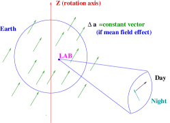
Figure 1: Schematic representation of searches for sidereal variations of the CPT-violating parameter $\delta_{K}$ in the SME framework. The green arrows, crossing the Earth indicate a constant Lorentz-violating vector that characterizes the Lorentz-violating ground state.

From the KTeV experiment [28] the following bounds on the $X$ and $Y$ components of the $a_{\mu}$ parameter have been obtained

$$\Delta a_{X},\Delta a_{Y}<9.2\times 10^{-22}~{}{\rm GeV}~{},$$

where $X,Y,Z$ denote sidereal coordinates (see Fig. 1).

Complementary probes of the $a_{Z}$ component can come from $\phi$-factories [23]. In the case of $\phi$-factories there is additional dependence of the CPT-violating parameter $\delta_{K}$ on the polar ($\theta$) and azimuthal ($\phi$) angles

$$\delta_{K}^{\phi}(|\vec{p}|,\theta,t)=\frac{1}{\pi}\int_{0}^{2\pi}d\phi\delta_{K}(\vec{p},t)\simeq$$

$$i{\rm sin}\widehat{\phi}{\rm exp}(i\widehat{\phi})(\gamma/\Delta m)\left(\Delta a_{0}+\beta_{K}\Delta{a_{Z}}{\rm cos}\chi{\rm cos}\theta+\right.$$

$$\left.\beta_{K}\Delta{a_{X}}{\rm sin}\chi{\rm cos}\theta{\rm cos}(\Omega t)+\beta_{K}\Delta{a_{Y}}{\rm sin}\chi{\rm cos}\theta{\rm sin}(\Omega t)\right)$$

where $\Omega$ denotes the Earth’s sidereal frequency, and $\chi$ is the angle between the laboratory Z-axis and the Earth’s axis.

The experiment KLOE at DA$\Phi$NE is sensitive to $a_{Z}$: limits on $\delta(\Delta a_{Z})$ can be placed from forward-backward asymmetry measurements $A_{L}=2{\rm Re}\epsilon_{K}-2{\rm Re}\delta_{K}$. For more details on the relevant experimental bounds we refer the reader to the literature [23].

We only mention at this stage that in an upgraded DA$\Phi$NE facility, namely experiment KLOE-2 at DA$\Phi$NE-2, the expected sensitivity is [23] $\Delta a_{\mu}={\cal O}(10^{-18})$ GeV which, however, is not competitive with the current KTeV limits on $a_{X,Y}$ given above.

We close this subsection by pointing out that additional precision tests can be performed using other meson factories (using B-mesons, etc.… ), which would also allow one to test the universality of QG Lorentz-violating effects, if observed.

3 QG Decoherence and CPTV in Neutral Kaons

3.1 Stochastically Fluctuating Geometries, Light Cone Fluctuations and Decoherence: General Ideas

If the ground state of QG consists of “fuzzy” space-time, i.e., stochastically-fluctuating metrics, then a plethora of interesting phenomena may occur, including light-cone fluctuations [29, 21] (c.f. Fig. 2). Such effects will lead to stochastic fluctuations in, say, arrival times of photons with common energy, which can be detected with high precision in astrophysical experiments [30, 29]. In addition, they may give rise to decoherence of matter, in the sense of induced time-dependent damping factors in the evolution equations of the (reduced) density matrix of matter fields [21, 31].

Figure 2: In stochastic space-time models of QG the light cone may fluctuate, leading to decoherence and quantum fluctuations of the speed of light in “vacuo”.

Such “fuzzy” space-times are formally represented by metric deviations which are fluctuating randomly about, say, flat Minkowski space-time: $g_{\mu\nu}=\eta_{\mu\nu}+h_{\mu\nu}$, with $\langle\cdots\rangle$ denoting statistical quantum averaging, and $\langle g_{\mu\nu}\rangle=\eta_{\mu\nu}$ but $\langle h_{\mu\nu}(x)h_{\lambda\sigma}(x^{\prime})\rangle\neq 0$, i.e., one has only quantum (light cone) fluctuations but not mean-field effects on dispersion relations of matter probes. In such a situation Lorentz symmetry is respected on the average, but not in individual measurements.

The path of light follows null geodesics $0=ds^{2}=g_{\mu\nu}dx^{\mu}dx^{\nu}$, with non-trivial fluctuations in geodesic deviations, ${D^{2}n^{\mu}\over D\tau^{2}}=-R^{\mu}_{\alpha\nu\beta}u^{\alpha}n^{\nu}u^{\beta}\,;$ in a standard general-relativistic notation, $D/D\tau$ denotes the appropriate covariant derivative operation, $R^{\mu}_{\alpha\nu\beta}$ the (fluctuating) Riemann curvature tensor, and $u^{\mu}$ ($n^{\mu}$) the tangential (normal) vector along the geodesic.

Such an effect causes primarily fluctuations in the arrival time of photons at the detector ($|\phi\rangle$=state of gravitons, $|0\rangle$= vacuum state)

$$\Delta t_{obs}^{2}=|\Delta t_{\phi}^{2}-\Delta t_{0}^{2}|={|\langle\phi|\sigma_{1}^{2}|\phi\rangle-\langle 0|\sigma_{1}^{2}|0\rangle|\over r^{2}}\equiv{|\langle\sigma_{1}^{2}\rangle_{R}|\over r}\,,$$

where

$$\langle\sigma_{1}^{2}\rangle_{R}=\frac{1}{8}(\Delta r)^{2}\int_{r_{0}}^{r_{1}}dr\int_{r_{0}}^{r_{1}}dr^{\prime}\>\,n^{\mu}n^{\nu}n^{\rho}n^{\sigma}\>\,$$

$$\langle\phi|h_{\mu\nu}(x)h_{\rho\sigma}(x^{\prime})+h_{\mu\nu}(x^{\prime})h_{\rho\sigma}(x)|\phi\rangle$$

and the two-point function of graviton fluctuations can be evaluated using standard field theory techniques [29].

Apart from the stochastic metric fluctuations, however, the aforementioned effects could also induce decoherence of matter propagating in these types of backgrounds [31], a possibility of particular interest for the purposes of the present article. Through the theorem of Wald [7], this implies that the CPT operator is not well-defined, and hence one also has a breaking of CPT symmetry.

We now proceed to describe briefly the general formalism used for parametrizing such QG-induced decoherence, as far as the CPT-violating effects on matter are concerned.

3.2 Formalism for the Phenomenology of QG-induced Decoherence

In this subsection we shall be very brief, giving the reader a flavor of the formalism underlying such decoherent systems. We shall discuss first a model-independent parametrization of decoherence, applicable not only to QG media, but covering a more general situation.

If the effects of the environment are such that the modified evolution equation of the (reduced) density matrix of matter $\rho$ [32] is linear, one can write down a Lindblad evolution equation [6], provided that (i) there is (complete) positivity of $\rho$, so that negative probabilities do not arise at any stage of the evolution, (ii) the energy of the matter system is conserved on the average, and (iii) the entropy is increasing monotonically.

For $N$-level systems, the generic decohering Lindblad evolution for $\rho$ reads

$$\frac{\partial\rho_{\mu}}{\partial t}=\sum_{ij}h_{i}\rho_{j}{f}_{ij\mu}+\sum_{\nu}{L}_{\mu\nu}\rho_{\nu}~{},$$

$$\quad~{}\mu,\nu=0,\dots N^{2}-1,\quad i,j=1,\dots N^{2}-1~{},$$

where the $h_{i}$ are Hamiltonian terms, expanded in an appropriate basis, and the decoherence matrix $L$ has the form: ${L}_{0\mu}={L}_{\mu 0}=0~{},$ ${L}_{ij}=\frac{1}{4}\sum_{k,\ell,m}c_{l\ell}\left(-f_{i\ell m}f_{kmj}+f_{kim}f_{\ell mj}\right)~{},$ with $c_{ij}$ a positive-definite matrix and $f_{ijk}$ the structure constants of the appropriate $SU(N)$ group. In this generic phenomenological description of decoherence, the elements ${L}_{\mu\nu}$ are free parameters, to be determined by experiment. We shall come back to this point in the next subsection, where we discuss neutral kaon decays.

A rather characteristic feature of this equation is the appearance of exponential damping, $e^{-(...)t}$, in interference terms of the pertinent quantities (for instance, matrix elements $\rho$, or asymmetries in the case of the kaon system, see below). The exponents are proportional to (linear combinations) of the elements of the decoherence matrix [6, 4, 32]. Note, however, that Lindblad type evolution is not the most generic evolution for QG models. In cases of space-time foam corresponding to stochastically (random) fluctuating space-times, such as the situations causing light-cone fluctuations examined previously, there is a different kind of decoherent evolution, with damping that is quadratic in time, i.e., one has a $e^{-(...)t^{2}}$ suppression of interference terms in the relevant observables.

A specific model of stochastic space-time foam is based on a particular kind of gravitational foam [21, 33, 31], consisting of “real” (as opposed to “virtual”) space-time defects in higher-dimensional space times, in accordance with the modern viewpoint of our world as a brane hyper-surface embedded in the bulk space-time [34]. This model is quite generic in some respects, and we will use it later to estimate the order of magnitude of novel CPT violating effects in entangled states of kaons.

A model of space-time foam [33] can be based on a number (determined by target-space supersymmetry) of parallel brane worlds with three large spatial dimensions. These brane worlds move in a bulk space-time, containing a “gas” of point-like bulk branes, termed “D-particles”, which are stringy space-time solitonic defects. One of these branes is the observable Universe. For an observer on the brane the crossing D-particles will appear as twinkling space-time defects, i.e. microscopic space-time fluctuations. This will give the four-dimensional brane world a “D-foamy” structure. Following work on gravitational decoherence [21, 31], the target-space metric state, which is close to being flat, can be represented schematically as a density matrix

$$\rho_{\mathrm{grav}}=\int d\,^{5}r\,\,f\left(r_{\mu}\right)\left|g\left(r_{\mu}\right)\right\rangle\left\langle g\left(r_{\mu}\,\right)\right|.\,$$ (7)

The parameters $r_{\mu}\,\left(\mu=0,1\ldots\right)$ pertain to appropriate space-time metric deformations and are stochastic, with a Gaussian distribution $\,f\left(r_{\mu}\,\right)$ characterized by the averages

$$\left\langle r_{\mu}\right\rangle=0,\;\left\langle r_{\mu}r_{\nu}\right\rangle=\Delta_{\mu}\delta_{\mu\nu}\,.$$

This model will be studied in more detail in section 4.

We will assume that the fluctuations of the metric felt by two entangled neutral mesons are independent, and $\Delta_{\mu}\sim O\left(\frac{E^{2}}{M_{P}^{2}}\right)$, i.e., very small. As matter moves through the space-time foam in a typical ergodic picture, the effect of time averaging is assumed to be equivalent to an ensemble average. For our present discussion we consider a semi-classical picture for the metric, and therefore $\left|g\left(r_{\mu}\right)\right\rangle$ in (7) is a coherent state.

In the specific model of foam discussed in [31], there is a recoil effect of the D-particle, as a result of its scattering with stringy excitations that live on the brane world and represent low-energy ordinary matter. As the space-time defects, propagating in the bulk space-time, cross the brane hyper-surface from the bulk in random directions, they scatter with matter. The associated distortion of space-time caused by this scattering can be considered dominant only along the direction of motion of the matter probe. Random fluctuations are then considered about an average flat Minkowski space-time. The result is an effectively two-dimensional approximate fluctuating metric describing the main effects [31]

$$g^{\mu\nu}=$$

$$\left(\begin{array}[]{cc}-(a_{1}+1)^{2}+a_{2}^{2}&-a_{3}(a_{1}+1)+a_{2}(a_{4}+1)\\ -a_{3}(a_{1}+1)+a_{2}(a_{4}+1)&-a_{3}^{2}+(a_{4}+1)^{2}\\ \end{array}\right).$$ (10)

(11)

The $a_{i}$ represent the fluctuations and are assumed to be random variables, satisfying $\langle a_{i}\rangle=0$ and $\langle a_{i}a_{j}\rangle=\delta_{ij}\sigma_{i}$.

Such a (microscopic) model of space-time foam is not of Lindblad type, as can be seen [31] by considering the oscillation probability for, say, two-level scalar systems describing oscillating neutral kaons, $K^{0}~{}\leftrightarrow\overline{K}^{0}$. In the approximation of small fluctuations one finds the following form for the oscillation probability of the two-level scalar system:

$$\langle e^{i(\omega_{1}-\omega_{2})t}\rangle=$$

$$\frac{4\tilde{d}^{2}}{(P_{1}P_{2})^{1/2}}\exp\left(\frac{\chi_{1}}{\chi_{2}}\right)\exp(i\tilde{b}t)\,,$$

where $\omega_{i},~{}i=1,2$ are the appropriate energy levels [31] of the two-level kaon system in the background of the fluctuating space-time (11), and

$$\chi_{1} = -4(\tilde{d}^{2}\sigma_{1}+\sigma_{4}k^{4})\tilde{b}^{2}t^{2}+2i\tilde{d}^{2}\widetilde{b}^{2}\widetilde{c}k^{2}\sigma_{1}\sigma_{4}t^{3},$$

$$\chi_{2} = 4\tilde{d}^{2}-2i\tilde{d}^{2}(k^{2}\tilde{c}\sigma_{4}+2\tilde{b}\sigma_{1})t+$$

$$\widetilde{b}k^{2}\left(\widetilde{b}k^{2}-2\widetilde{d}^{2}\widetilde{c}\right)\sigma_{1}\sigma_{4},$$

$$P_{1} = 4\tilde{d}^{2}+2i\widetilde{d}\widetilde{b}\left(k^{2}-\widetilde{d}\right)\sigma_{2}t+\tilde{b}^{2}k^{4}\sigma_{2}\sigma_{3}t^{2},$$

$$P_{2} = 4\tilde{d}^{2}-2i\widetilde{d}^{2}\left(k^{2}\widetilde{c}\sigma_{4}+2\widetilde{b}\sigma_{1}\right)t+\mathcal{O}\left(\sigma^{2}\right)~{},$$

with

$$\begin{array}[]{c}\tilde{b}=\sqrt{k^{2}+m_{1}^{2}}-\sqrt{k^{2}+m_{2}^{2}},\\ \tilde{c}=m_{1}^{2}(k^{2}+m_{1}^{2})^{-3/2}-m_{2}^{2}(k^{2}+m_{2}^{2})^{-3/2},\\ \tilde{d}=\sqrt{k^{2}+m_{1}^{2}}\sqrt{k^{2}+m_{2}^{2}}.\end{array}$$

From this expression one can see [31] that the stochastic model of space-time foam leads to a modification of oscillation behavior quite distinct from that of the Lindblad formulation. In particular, the transition probability displays a Gaussian time-dependence, decaying as $e^{-(...)t^{2}}$, a modification of the oscillation period, as well as additional power-law fall-off.

From this characteristic time-dependence, one can obtain bounds for the fluctuation strength of space-time foam in kaon systems. In the context of this presentation, we restrict ourselves to Lindblad decoherence tests using only neutral kaons. However, when discussing the CPTV effects of foam on entangled states we make use of this specific model of stochastically fluctuating D-particle foam [33, 31], in order to demonstrate the effects explicitly and obtain definite order-of-magnitude estimates [35].

3.3 Experiments involving Single-Kaon States

As mentioned in the previous subsection, QG may induce decoherence and oscillations $K^{0}\leftrightarrow{\overline{K}}^{0}$ [4, 8], thereby implying a two-level quantum mechanical system interacting with a QG “environment”. Adopting the general assumptions of average energy conservation and monotonic entropy increase, the simplest model for parametrizing decoherence (in a rather model-independent way) is the (linear) Lindblad approach mentioned earlier. Not all entries of a general decoherence matrix are physical, and in order to isolate the physically relevant entries one must invoke specific assumptions, related to the symmetries of the particle system in question. For the neutral kaon system, such an extra assumptions is that the QG medium respects the $\Delta S=\Delta Q$ rule. In such a case, the modified Lindblad evolution equation (4) for the respective density matrices of neutral kaon matter can be parametrized as follows [4]:

$$\partial_{t}\rho=i[\rho,H]+\delta H\hskip-8.5pt/\hskip 2.0pt\rho~{},$$

where

$$H_{\alpha\beta}=\left(\begin{array}[]{cccc}-\Gamma&-{\textstyle{1\over 2}}\delta\Gamma&-{\rm Im}\Gamma_{12}&-{\rm Re}\Gamma_{12}\\ -{\textstyle{1\over 2}}\delta\Gamma&-\Gamma&-2{\rm Re}M_{12}&-2{\rm Im}M_{12}\\ -{\rm Im}\Gamma_{12}&2{\rm Re}M_{12}&-\Gamma&-\delta M\\ -{\rm Re}\Gamma_{12}&-2{\rm Im}M_{12}&\delta M&-\Gamma\end{array}\right)$$

and

$${\delta H\hskip-8.5pt/\hskip 2.0pt}_{\alpha\beta}=\left(\begin{array}[]{cccc}0&0&0&0\\ 0&0&0&0\\ 0&0&-2\alpha&-2\beta\\ 0&0&-2\beta&-2\gamma\end{array}\right)~{}.$$

Positivity of $\rho$ requires: $\alpha,\gamma>0,\quad\alpha\gamma>\beta^{2}$. Notice that $\alpha,\beta,\gamma$ violate both CPT, due to their decohering nature [7], and CP symmetry, as they do not commute with the CP operator $\widehat{CP}$ [8]: $\widehat{CP}=\sigma_{3}\cos\theta+\sigma_{2}\sin\theta$,$~{}~{}~{}~{}~{}[\delta H\hskip-8.5pt/\hskip 2.0pt_{\alpha\beta},\widehat{CP}]\neq 0$.

An important remark is now in order. As pointed out in [10], although the above parametrization is sufficient for a single-kaon state to have a positive definite density matrix (and hence probabilities) this is not true when one considers the evolution of entangled kaon states ($\phi$-factories). In this latter case, complete positivity is guaranteed only if the further conditions

$$\alpha=\gamma~{}{\rm and}~{}\beta=0$$ (13)

are imposed. When incorporating entangled states, one should either consider possible new effects (such as the $\omega$-effect considered below) or apply the constraints (13) also to single kaon states [10]. This is not necessarily the case when other non-entangled particle states, such as neutrinos, are considered, in which case the $\alpha,\beta,\gamma$ parametrization of decoherence may be applied. Experimentally the complete positivity hypothesis can be tested explicitly. In what follows, as far as single-kaon states are concerned, we keep the $\alpha,\beta,\gamma$ parametrization, and give the available experimental bounds for them, but we always have in mind the constraint (13) when referring to entangled kaon states in a $\phi$-factory.

As already mentioned, when testing CPT symmetry with neutral kaons one should be careful to distinguish two types of CPTV: (i) CPTV within Quantum Mechanics [11], leading to possible differences between particle-antiparticle masses and widths: $\delta m=m_{K^{0}}-m_{{\overline{K}}^{0}}$, $\delta\Gamma=\Gamma_{K^{0}}-\Gamma_{{\overline{K}}^{0}}$. This type of CPTV could be, for instance, due to (spontaneous) Lorentz violation [13]. In that case the CPT operator is well-defined as a quantum mechanical operator, but does not commute with the Hamiltonian of the system. This, in turn, may lead to mass and width differences between particles and antiparticles, among other effects. (ii) CPTV through decoherence [4, 5] via the parameters $\alpha,\beta,\gamma$ (entanglement with the QG “environment”, leading to modified evolution for $\rho$ and $\$\neq S~{}S^{\dagger}$). In the latter case the CPT operator may not be well-defined, which implies novel effects when one uses entangled states of kaons, as we shall discuss in the next subsection.

Figure 3: Neutral kaon decay asymmetries $A_{2\pi}$ [8] indicating the effects of QG-induced decoherence.

Figure 4: Typical neutral kaon decay asymmetries $A_{\Delta m}$ [8] indicating the effects of QG-induced decoherence.

Figure 5: Typical neutral kaon decay asymmetries $A_{T}$ [8] indicating the effects of QG-induced decoherence.

Process	QMV	QM
$A_{2\pi}$	$\not=$	$\not=$
$A_{3\pi}$	$\not=$	$\not=$
$A_{\rm T}$	$\not=$	$=$
$A_{\rm CPT}$	$=$	$\not=$
$A_{\Delta m}$	$\not=$	$=$
$\zeta$	$\not=$	$=$

Table 1: Qualitative comparison of predictions for various observables in CPT-violating theories beyond (QMV) and within (QM) quantum mechanics. Predictions either differ ($\not=$) or agree ($=$) with the results obtained in conventional quantum-mechanical CP violation. Note that these frameworks can be qualitatively distinguished via their predictions for $A_{\rm T}$, $A_{\rm CPT}$, $A_{\Delta m}$, and $\zeta$.

 

The important point to notice is that the two types of CPTV can be disentangled experimentally [8]. The relevant observables are defined as $\left\langle O_{i}\right\rangle={\rm Tr}\,[O_{i}\rho]$. For neutral kaons, one looks at decay asymmetries for $K^{0},{\overline{K}}^{0}$, defined as:

$$A(t)=\frac{R({\bar{K}}^{0}_{t=0}\rightarrow{\bar{f}})-R(K^{0}_{t=0}\rightarrow f)}{R({\bar{K}}^{0}_{t=0}\rightarrow{\bar{f}})+R(K^{0}_{t=0}\rightarrow f)}~{},$$

where $R(K^{0}\rightarrow f)\equiv{\rm Tr}\,[O_{f}\rho(t)]=$ denotes the decay rate into the final state $f$ (starting from a pure $K^{0}$ state at $t=0$).

In the case of neutral kaons, one may consider the following set of asymmetries: (i) identical final states: $f={\bar{f}}=2\pi$: $A_{2\pi}~{},~{}A_{3\pi}$, (ii) semileptonic : $A_{T}$ (final states $f=\pi^{+}l^{-}\bar{\nu}\ \not=\ \bar{f}=\pi^{-}l^{+}\nu$), $A_{CPT}$ (${\overline{f}}=\pi^{+}l^{-}\bar{\nu},~{}f=\pi^{-}l^{+}\nu$), $A_{\Delta m}$. Typically, for instance when final states are $2\pi$, one has a time evolution of the decay rate $R_{2\pi}$: $R_{2\pi}(t)=c_{S}\,e^{-\Gamma_{S}t}+c_{L}\,e^{-\Gamma_{L}t}+2c_{I}\,e^{-\Gamma t}\cos(\Delta mt-\phi)$, where $S$=short-lived, $L$=long-lived, $I$=interference term, $\Delta m=m_{L}-m_{S}$, $\Delta\Gamma=\Gamma_{S}-\Gamma_{L}$, $\Gamma=\frac{1}{2}(\Gamma_{S}+\Gamma_{L})$. One may define the decoherence parameter $\zeta=1-{c_{I}\over\sqrt{c_{S}c_{L}}}$, as a (phenomenological) measure of quantum decoherence induced in the system [11]. For larger sensitivities one can look at this parameter in the presence of a regenerator [8]. In our decoherence scenario, $\zeta$ corresponds to a particular combination of the decoherence parameters [8]:

$$\zeta\to\frac{\widehat{\gamma}}{2|\epsilon^{2}|}-2\frac{{\widehat{\beta}}}{|\epsilon|}{\rm sin}\phi~{},$$

with the notation $\widehat{\gamma}=\gamma/\Delta\Gamma$, etc. Hence, ignoring the constraint (13), the best bounds on $\beta$, or -turning the logic around- the most sensitive tests of complete positivity in kaons, can be placed by implementing a regenerator [8].

The experimental tests (decay asymmetries) that can be performed in order to disentangle decoherence from quantum-mechanical CPT violating effects are summarized in Table 1. In Figures 3, 4, 5 we give typical profiles of several decay asymmetries [8], from where bounds on QG decohering parameters can be extracted. At present there are experimenatl bounds available from CPLEAR measurements [36] $\alpha<4.0\times 10^{-17}~{}{\rm GeV}~{},~{}|\beta|<2.3.\times 10^{-19}~{}{\rm GeV}~{},~{}\gamma<3.7\times 10^{-21}~{}{\rm GeV}$, which are not much different from theoretically expected values in some optimistic scenarios [8] $\alpha~{},\beta~{},\gamma=O(\xi\frac{E^{2}}{M_{P}})$.

Recently, the experiment KLOE at DA$\Phi$NE updated these limits by measuring for the first time the $\gamma$ decoherence parameter for entangled kaon states [23], as well as the (naive) decoherence parameter $\zeta$ (to be specific, the KLOE Collaboration has presented measurements for two $\zeta$ parameters, one, $\zeta_{LS}$, pertaining to an expansion in terms of $K_{L},K_{S}$ states, and the other, $\zeta_{0\bar{0}}$, for an expansion in terms of $K^{0},\overline{K}^{0}$ states). We remind the reader once more that, under the assumption of complete positivity for entangled meson states [10], theoretically there is only one parameter to parametrize Lindblad decoherence, since $\alpha=\gamma$, $\beta=0$. In fact, the KLOE experiment has the greatest sensitivity to this parameter $\gamma$. The latest KLOE measurement [23] for $\gamma$ yields $\gamma_{\rm KLOE}=(1.1^{+2.9}_{-2.4}\pm 0.4)\times 10^{-21}~{}{\rm GeV}$, i.e. $\gamma<6.4\times 10^{-21}~{}{\rm GeV}$, competitive with the corresponding CPLEAR bound [36] discussed above. It is expected that this bound could be improved by an order of magnitude in upgraded facilities, such as KLOE-2 at DA$\Phi$NE-2 [23], where one expects $\gamma_{\rm upgrade}\to\pm 0.2\times 10^{-21}~{}{\rm GeV}$.

The reader should also bear in mind that the Lindblad linear decoherence is not the only possibility for a parametrization of QG effects, see for instance the stochastically fluctuating space-time metric approach discussed in Section 3.1 above. Thus, direct tests of the complete positivity hypothesis in entangled states, and hence the theoretical framework per se, should be performed by independent measurements of all the three decoherence parameters $\alpha,\beta,\gamma$; as far as we understand , such data are currently available in kaon factories, but not yet analyzed in detail [23].

4 CPTV and Modified EPR Correlations of Entangled Neutral Kaon States

4.1 EPR Correlations in Particle Physics

We now come to a description of an entirely novel effect [12] of CPTV due to the ill-defined nature of the CPT operator, which is exclusive to neutral-meson factories, for reasons explained below. The effects are qualitatively similar for kaon and $B$-meson factories [37], with the important observation that in kaon factories there is a particularly good channel, that of both correlated kaons decaying to $\pi^{+}\pi^{-}$. In that channel the sensitivity of the effect increases because the complex parameter $\omega$, parametrizing the relevant EPR modifications [12], appears in the particular combination $|\omega|/|\eta_{+-}|$, with $|\eta_{+-}|\sim 10^{-3}$. In the case of $B$-meson factories one should focus instead on the “same-sign” di-lepton channel [37], where high statistics is expected.

In this article we restrict ourselves to the case of $\phi$-factories, referring the interested reader to the literature [37] for the $B$-meson applications. We commence our discussion by briefly reminding the reader of EPR particle correlations.

The EPR effect was originally proposed as a paradox, testing the foundations of Quantum Theory. There was the question whether quantum correlations between spatially separated events implied instant transport of information that would contradict special relativity. It was eventually realized that no super-luminal propagation was actually involved in the EPR phenomenon, and thus there was no conflict with relativity.

Figure 6: Schematic representation of the decay of a $\phi$-meson at rest (for definiteness) into pairs of entangled neutral kaons, which eventually decay on the two sides of the detector.

The EPR effect has been confirmed experimentally, e.g., in meson factories: (i) a pair of particles can be created in a definite quantum state, (ii) move apart and, (iii) eventually decay when they are widely (spatially) separated (see Fig. 6 for a schematic representation of an EPR effect in a meson factory). Upon making a measurement on one side of the detector and identifying the decay products, we infer the type of products appearing on the other side; this is essentially the EPR correlation phenomenon. It does not involve any simultaneous measurement on both sides, and hence there is no contradiction with special relativity. As emphasized by Lipkin [38], the EPR correlations between different decay modes should be taken into account when interpreting any experiment.

4.2 CPTV and Modified EPR-Correlations in $\phi$ Factories: the $\omega$-Effect

In the case of $\phi$ factories it was claimed  [39] that due to EPR correlations, irrespective of CP, and CPT violation, the final state in $\phi$ decays: $e^{+}e^{-}\Rightarrow\phi\Rightarrow K_{S}K_{L}$ always contains $K_{L}K_{S}$ products. This is a direct consequence of imposing the requirement of Bose statistics on the state $K^{0}{\overline{K}}^{0}$ (to which the $\phi$ decays); this, in turn, implies that the physical neutral meson-antimeson state must be symmetric under C${\cal P}$, with C the charge conjugation and ${\cal P}$ the operator that permutes the spatial coordinates. Assuming conservation of angular momentum, and a proper existence of the antiparticle state (denoted by a bar), one observes that: for $K^{0}{\overline{K}}^{0}$ states which are C-conjugates with C$=(-1)^{\ell}$ (with $\ell$ the angular momentum quantum number), the system has to be an eigenstate of the permutation operator ${\cal P}$ with eigenvalue $(-1)^{\ell}$. Thus, for $\ell=1$: C$=-$ $\rightarrow{\cal P}=-$. Bose statistics ensures that for $\ell=1$ the state of two identical bosons is forbidden. Hence, the initial entangled state:

$$|i>=\frac{1}{\sqrt{2}}\left(|K^{0}({\vec{k}}),{\overline{K}}^{0}(-{\vec{k}})>-|{\overline{K}}^{0}({\vec{k}}),{K}^{0}(-{\vec{k}})>\right)$$

$$={\cal N}\left(|K_{S}({\vec{k}}),K_{L}(-{\vec{k}})>-|K_{L}({\vec{k}}),K_{S}(-{\vec{k}})>\right)$$

with the normalization factor ${\cal N}=\frac{\sqrt{(1+|\epsilon_{1}|^{2})(1+|\epsilon_{2}|^{2})}}{\sqrt{2}(1-\epsilon_{1}\epsilon_{2})}\simeq\frac{1+|\epsilon^{2}|}{\sqrt{2}(1-\epsilon^{2})}$, and $K_{S}=\frac{1}{\sqrt{1+|\epsilon_{1}^{2}|}}\left(|K_{+}>+\epsilon_{1}|K_{-}>\right)$, $K_{L}=\frac{1}{\sqrt{1+|\epsilon_{2}^{2}|}}\left(|K_{-}>+\epsilon_{2}|K_{+}>\right)$, where $\epsilon_{1},\epsilon_{2}$ are complex parameters, such that $\epsilon\equiv\epsilon_{1}+\epsilon_{2}$ denotes the CP- & T-violating parameter, whilst $\delta\equiv\epsilon_{1}-\epsilon_{2}$ parametrizes the CPT & CP violation within quantum mechanics [11], as discussed previously. The $K^{0}\leftrightarrow{\overline{K}}^{0}$ or $K_{S}\leftrightarrow K_{L}$ correlations are apparent after evolution, at any time $t>0$ (with $t=0$ taken as the moment of the $\phi$ decay).

In the above considerations there is an implicit assumption, which was noted in [12]. The above arguments are valid independently of CPTV, provided such violation occurs within quantum mechanics, e.g., due to spontaneous Lorentz violation, where the CPT operator is well defined.

If, however, CPT is intrinsically violated, due, for instance, to decoherence scenarios in space-time foam, then the factorizability property of the super-scattering matrix $ breaks down, $ $\neq SS^{\dagger}$, and the generator of CPT is not well defined [7]. Thus, the concept of an “antiparticle” may be modified perturbatively! The perturbative modification of the properties of the antiparticle is important, since the antiparticle state is a physical state which exists, despite the ill-definition of the CPT operator. However, the antiparticle Hilbert space will have components that are independent of the particle Hilbert space.

In such a case, the neutral mesons $K^{0}$ and ${\overline{K}}^{0}$ should no longer be treated as indistinguishable particles. As a consequence [12], the initial entangled state in $\phi$ factories $|i>$, after the $\phi$-meson decay, will acquire a component with opposite permutation (${\cal P}$) symmetry:

$$|i> = \frac{1}{\sqrt{2}}\left(|K_{0}({\vec{k}}),{\overline{K}}_{0}(-{\vec{k}})>-|{\overline{K}}_{0}({\vec{k}}),K_{0}(-{\vec{k}})>\right)$$

$$+ \frac{\omega}{2}\left(|K_{0}({\vec{k}}),{\overline{K}}_{0}(-{\vec{k}})>+|{\overline{K}}_{0}({\vec{k}}),K_{0}(-{\vec{k}})>\right)\bigg{]}$$

$$= \bigg{[}{\cal N}\left(|K_{S}({\vec{k}}),K_{L}(-{\vec{k}})>-|K_{L}({\vec{k}}),K_{S}(-{\vec{k}})>\right)$$

$$+ \omega\left(|K_{S}({\vec{k}}),K_{S}(-{\vec{k}})>-|K_{L}({\vec{k}}),K_{L}(-{\vec{k}})>\right)\bigg{]}~{},$$

where ${\cal N}$ is an appropriate normalization factor, and $\omega=|\omega|e^{i\Omega}$ is a complex parameter, parametrizing the intrinsic CPTV modifications of the EPR correlations. Notice that, as a result of the $\omega$-terms, there exist, in the two-kaon state, $K_{S}K_{S}$ or $K_{L}K_{L}$ combinations, which entail important effects to the various decay channels. Due to this effect, termed the $\omega$-effect by the authors of [12], there is contamination of ${\cal P}$(odd) state with ${\cal P}$(even) terms. The $\omega$-parameter controls the amount of contamination of the final ${\cal P}$(odd) state by the “wrong” (${\cal P}$(even)) symmetry state.

Later in this section we will present a microscopic model where such a situation is realized explicitly. Specifically, an $\omega$-like effect appears due to the evolution in the space-time foam, and the corresponding parameter turns out to be purely imaginary and time-dependent [35].

4.3 $\omega$-Effect Observables

To construct the appropriate observable for the possible detection of the $\omega$-effect, we consider the $\phi$-decay amplitude depicted in Fig. 6, where one of the kaon products decays to the final state $X$ at $t_{1}$ and the other to the final state $Y$ at time $t_{2}$. We take $t=0$ as the moment of the $\phi$-meson decay.

The relevant amplitudes read:

$$A(X,Y)=\langle X|K_{S}\rangle\langle Y|K_{S}\rangle\,{\cal N}\,\left(A_{1}+A_{2}\right)~{},$$

with

$$A_{1} = e^{-i(\lambda_{L}+\lambda_{S})t/2}[\eta_{X}e^{-i\Delta\lambda\Delta t/2}-\eta_{Y}e^{i\Delta\lambda\Delta t/2}]$$

$$A_{2} = \omega[e^{-i\lambda_{S}t}-\eta_{X}\eta_{Y}e^{-i\lambda_{L}t}]$$

denoting the CPT-allowed and CPT-violating parameters respectively, and $\eta_{X}=\langle X|K_{L}\rangle/\langle X|K_{S}\rangle$ and $\eta_{Y}=\langle Y|K_{L}\rangle/\langle Y|K_{S}\rangle$. In the above formulae, $t$ is the sum of the decay times $t_{1},t_{2}$ and $\Delta t$ is their difference (assumed positive).

Figure 7: A characteristic case of the intensity $I(\Delta t)$, with $|\omega|=0$ (solid line) vs $I(\Delta t)$ (dashed line) with $|\omega|=|\eta_{+-}|$, $\Omega=\phi_{+-}-0.16\pi$, for definiteness [12].

The “intensity” $I(\Delta t)$ is the desired observable for a detection of the $\omega$-effect,

$$I(\Delta t)\equiv\frac{1}{2}\int_{\Delta t}^{\infty}dt\,|A(X,Y)|^{2}~{}.$$

depending only on $\Delta t$.

Its time profile reads [12]:

$$I(\Delta t)\equiv\frac{1}{2}\int_{|\Delta t|}^{\infty}dt\,|A(\pi^{+}\pi^{-},\pi^{+}\pi^{-})|^{2}=$$

$$|\langle\pi^{+}\pi^{-}|K_{S}\rangle|^{4}|{\cal N}|^{2}|\eta_{+-}|^{2}\bigg{[}I_{1}+I_{2}+I_{12}\bigg{]}~{},$$

where

$$I_{1}(\Delta t)=\frac{e^{-\Gamma_{S}\Delta t}+e^{-\Gamma_{L}\Delta t}-2e^{-(\Gamma_{S}+\Gamma_{L})\Delta t/2}\cos(\Delta m\Delta t)}{\Gamma_{L}+\Gamma_{S}}$$

$$I_{2}(\Delta t)=\frac{|\omega|^{2}}{|\eta_{+-}|^{2}}\frac{e^{-\Gamma_{S}\Delta t}}{2\Gamma_{S}}$$

$$I_{12}(\Delta t)=-\frac{4}{4(\Delta m)^{2}+(3\Gamma_{S}+\Gamma_{L})^{2}}\frac{|\omega|}{|\eta_{+-}|}\times$$

$$\bigg{[}2\Delta m\bigg{(}e^{-\Gamma_{S}\Delta t}\sin(\phi_{+-}-\Omega)-$$

$$e^{-(\Gamma_{S}+\Gamma_{L})\Delta t/2}\sin(\phi_{+-}-\Omega+\Delta m\Delta t)\bigg{)}$$

$$-(3\Gamma_{S}+\Gamma_{L})\bigg{(}e^{-\Gamma_{S}\Delta t}\cos(\phi_{+-}-\Omega)-$$

$$e^{-(\Gamma_{S}+\Gamma_{L})\Delta t/2}\cos(\phi_{+-}-\Omega+\Delta m\Delta t)\bigg{)}\bigg{]}~{},$$

with $\Delta m=m_{S}-m_{L}$ and $\eta_{+-}=|\eta_{+-}|e^{i\phi_{+-}}$ in the usual notation [11].

A typical case for the relevant intensities, indicating clearly the novel CPTV $\omega$-effects, is depicted in Fig. 7.

As announced, the novel $\omega$-effect appears in the combination $\frac{|\omega|}{|\eta_{+-}|}$, thereby implying that the decay channel to $\pi^{+}\pi^{-}$ is particularly sensitive to the $\omega$ effect [12], due to the enhancement by $1/|\eta_{+-}|\sim 10^{3}$, implying sensitivities up to $|\omega|\sim 10^{-6}$ in $\phi$ factories. The physical reason for this enhancement is that $\omega$ enters through $K_{S}K_{S}$ as opposed to $K_{L}K_{S}$ terms, and the $K_{L}\to\pi^{+}\pi^{-}$ decay is CP-violating.

4.4 Microscopic Models for the $\omega$-Effect and Order-of-Magnitude Estimates

For future experimental searches for the $\omega$-effect it is important to estimate its expected order of magnitude, at least in some models of foam.

A specific model is that of the D-particle foam [33, 31, 35], discussed already in connection with the stochastic metric-fluctuation approach to decoherence. An important feature for the appearance of an $\omega$-like effect is that, during each scattering with a D-particle defect, there is (momentary) capture of the string state (representing matter) by the defect, and a possible change in phase and/or flavour for the particle state emerging from such a capture (see Fig. 8).

Figure 8: Upper: Recoil of closed string states with D-particles (space-time defects). Lower: A supersymmetric brane world model of D-particle foam. In both cases the recoil of (massive) D-particle defect causes distortion of space-time, stochastic metric fluctuations are possible and the emergent post-recoil string state may differ by flavour and CP phases.

The induced metric distortions, including such flavour changes for the emergent post-recoil matter state, are:

$$g^{00}=\left(-1+r_{4}\right)\mathsf{1}~{},$$

$$g^{01}=g^{10}=r_{0}\mathsf{1}+r_{1}\sigma_{1}+r_{2}\sigma_{2}+r_{3}\sigma_{3},$$

$$g^{11}=\left(1+r_{5}\right)\mathsf{1}$$

where the $\sigma_{i}$ are Pauli matrices.

The target-space metric state is the density matrix $\rho_{\mathrm{grav}}$ defined at (7) [35], with the same assumptions for the parameters $r_{\mu}$ stated there. The order of magnitude of the metric elements $g_{0i}\simeq\overline{v}_{i,rec}\propto g_{s}\frac{\Delta p_{i}}{M_{s}}$, where $\Delta p_{i}\sim{\tilde{\xi}}p_{i}$ is the momentum transfer during the scattering of the particle probe (kaon) with the D-particle defect, $g_{s}<1$ is the string coupling, assumed weak, and $M_{s}$ is the string scale, which in the modern approach to string/brane theory is not necessarily identified with the four-dimensional Planck scale, and is left as a phenomenological parameter to be constrained by experiment.

To estimate the order of magnitude of the $\omega$-effect we construct the gravitationally-dressed initial entangled state using stationary perturbation theory for degenerate states [12], the degeneracy being provided by the CP-violating effects. As Hamiltonian function we use

$$\widehat{H}=g^{01}\left(g^{00}\right)^{-1}\widehat{k}-\left(g^{00}\right)^{-1}\sqrt{\left(g^{01}\right)^{2}{k}^{2}-g^{00}\left(g^{11}k^{2}+m^{2}\right)}$$

describing propagation in the above-described stochastically-fluctuating space-time. To leading order in the variables $r$ the interaction Hamiltonian reads:

$$\widehat{H_{I}}=-\left({r_{1}\sigma_{1}+r_{2}\sigma_{2}}\right)\widehat{k}$$

with the notation $\left|K_{L}\right\rangle=\left|\uparrow\right\rangle~{},\quad\left|K_{S}\right\rangle=\left|\downarrow\right\rangle.$ The gravitationally-dressed initial states then can be constructed using stationary perturbation theory:

$$\left|k^{\left(i\right)},\downarrow\right\rangle_{QG}^{\left(i\right)}=\left|k^{\left(i\right)},\downarrow\right\rangle^{\left(i\right)}+\left|k^{\left(i\right)},\uparrow\right\rangle^{\left(i\right)}\alpha^{\left(i\right)}~{},$$

where $\alpha^{\left(i\right)}=\frac{{}^{\left(i\right)}\left\langle\uparrow,k^{\left(i\right)}\right|\widehat{H_{I}}\left|k^{\left(i\right)},\downarrow\right\rangle^{\left(i\right)}}{E_{2}-E_{1}}$. For $\left|{k^{\left(i\right)},\uparrow}\right\rangle^{\left(i\right)}$ the dressed state is obtained by $\left|\downarrow\right\rangle\leftrightarrow\left|\uparrow\right\rangle$ and $\alpha\to\beta$ where $\beta^{\left(i\right)}=\frac{{}^{\left(i\right)}\left\langle\downarrow,k^{\left(i\right)}\right|\widehat{H_{I}}\left|k^{\left(i\right)},\uparrow\right\rangle^{\left(i\right)}}{E_{1}-E_{2}}$.

The totally antisymmetric “gravitationally-dressed” state of two mesons (kaons) is then:

$$\begin{array}[c]{l}\left|{k,\uparrow}\right\rangle_{QG}^{\left(1\right)}\left|{-k,\downarrow}\right\rangle_{QG}^{\left(2\right)}-\left|{k,\downarrow}\right\rangle_{QG}^{\left(1\right)}\left|{-k,\uparrow}\right\rangle_{QG}^{\left(2\right)}=\\ \left|{k,\uparrow}\right\rangle^{\left(1\right)}\left|{-k,\downarrow}\right\rangle^{\left(2\right)}-\left|{k,\downarrow}\right\rangle^{\left(1\right)}\left|{-k,\uparrow}\right\rangle^{\left(2\right)}\\ +\left|{k,\downarrow}\right\rangle^{\left(1\right)}\left|{-k,\downarrow}\right\rangle^{\left(2\right)}\left({\beta^{\left(1\right)}-\beta^{\left(2\right)}}\right)+\\ \left|{k,\uparrow}\right\rangle^{\left(1\right)}\left|{-k,\uparrow}\right\rangle^{\left(2\right)}\left({\alpha^{\left(2\right)}-\alpha^{\left(1\right)}}\right)\\ +\beta^{\left(1\right)}\alpha^{\left(2\right)}\left|{k,\downarrow}\right\rangle^{\left(1\right)}\left|{-k,\uparrow}\right\rangle^{\left(2\right)}-\alpha^{\left(1\right)}\beta^{\left(2\right)}\left|{k,\uparrow}\right\rangle^{\left(1\right)}\left|{-k,\downarrow}\right\rangle^{\left(2\right)}~{}.\\ \end{array}$$

Notice here that, for our order-of-magnitude estimates, it suffices to assume that the initial entangled state of kaons is a pure state. In practice, due to the omnipresence of foam, this may not be entirely true, but this should not affect our order-of-magnitude estimates based on such an assumption.

With these remarks in mind we then write for the initial state of two kaons after the $\phi$ decay:

$$\left|\psi\right\rangle=\left|k,\uparrow\right\rangle^{\left(1\right)}\left|-k,\downarrow\right\rangle^{\left(2\right)}-\left|k,\downarrow\right\rangle^{\left(1\right)}\left|-k,\uparrow\right\rangle^{\left(2\right)}+$$

$$\xi\left|k,\uparrow\right\rangle^{\left(1\right)}\left|-k,\uparrow\right\rangle^{\left(2\right)}+\xi^{\prime}\left|k,\downarrow\right\rangle^{\left(1\right)}\left|-k,\downarrow\right\rangle^{\left(2\right)}~{},$$

where for $r_{i}\propto\delta_{i1}$ we have $\xi=\xi^{\prime}$, that is strangeness violation, whilst for $r_{i}\propto\delta_{i2}$ $\longrightarrow$ $\xi=-\xi^{\prime}$) (since $\alpha^{\left(i\right)}=\beta^{\left(i\right)})$ we obtain a strangeness conserving $\omega$-effect.

Upon averaging the density matrix over $r_{i}$, only the $|\omega|^{2}$ terms survive:

$$|\omega|^{2}=\mathcal{O}\left(\frac{1}{(E_{1}-E_{2})^{2}}(\langle\downarrow,k|H_{I}|k,\uparrow\rangle)^{2}\right)\sim$$

$$\frac{\Delta_{2}k^{2}}{(m_{1}-m_{2})^{2}}$$

for momenta of order of the rest energies, as is the case of a $\phi$ factory.

Recalling that in the recoil D-particle model under consideration we have [21, 35] $\Delta_{2}={\tilde{\xi}}^{2}k^{2}/M_{P}^{2}$, we obtain the following order of magnitude estimate of the $\omega$ effect:

$$|\omega|^{2}\sim\frac{{\tilde{\xi}}^{2}k^{4}}{M_{P}^{2}(m_{1}-m_{2})^{2}}~{}.$$ (15)

For neutral kaons with momenta of the order of the rest energies $|\omega|\sim 10^{-4}|{\tilde{\xi}}|$. For $1>{\tilde{\xi}}\geq 10^{-2}$ this not far below the sensitivity of current facilities, such as KLOE at DA$\Phi$NE. In fact, the KLOE experiment has just released the first measurement of the $\omega$ parameter [23]:

$${\rm Re}(\omega)=\left(1.1^{+8.7}_{-5.3}\pm 0.9\right)\times 10^{-4}~{},$$

$${\rm Im}(\omega)=\left(3.4^{+4.8}_{-5.0}\pm 0.6\right)\times 10^{-4}~{}.$$

One can constrain the $\omega$ parameter (or, in the context of the above specific model, the momentum-transfer parameter ${\tilde{\xi}}$) significantly in upgraded facilities. For instance, there are the following perspectives for KLOE-2 at (the upgraded) DA$\Phi$NE-2 [23]: ${\rm Re}(\omega),~{}{\rm Im}(\omega)\longrightarrow 2\times 10^{-5}$.

Let us now mention that $\omega$-like effects can also be generated by the Hamiltonian evolution of the system as a result of gravitational medium interactions. To this end, let us consider the Hamiltonian evolution in our stochastically-fluctuating D-particle-recoil distorted space-times, $\left|\psi\left(t\right)\right\rangle=\exp\left[-i\left(\widehat{H}^{(1)}+\widehat{H}^{\left(2\right)}\right)\frac{t}{\hbar}\right]\left|\psi\right\rangle$.

Assuming for simplicity $\xi=\xi^{\prime}=0$, it is easy to see [35] that the time-evolved state of two kaons contains strangeness-conserving $\omega$-terms:

$$\left|\psi\left(t\right)\right\rangle\sim e^{-i\left(\lambda_{0}^{\left(1\right)}+\lambda_{0}^{\left(2\right)}\right)t}\varpi\left(t\right)\times$$

$$\left\{\left|k,\uparrow\right\rangle^{\left(1\right)}\left|-k,\uparrow\right\rangle^{\left(2\right)}-\left|k,\downarrow\right\rangle^{\left(1\right)}\left|-k,\downarrow\right\rangle^{\left(2\right)}\right\}~{}.$$

The quantity $\varpi(t)$ obtained within this specific model is purely imaginary,

$${\cal O}\left(\varpi\right)\simeq i\frac{2\Delta_{1}^{\frac{1}{2}}k}{\left(k^{2}+m_{1}^{2}\right)^{\frac{1}{2}}-\left(k^{2}+m_{2}^{2}\right)^{\frac{1}{2}}}\times$$

$$\cos\left(\left|\lambda^{\left(1\right)}\right|t\right)\sin\left(\left|\lambda^{\left(1\right)}\right|t\right)=\varpi_{0}\sin\left(2\left|\lambda^{\left(1\right)}\right|t\right),$$

with $\Delta_{1}^{1/2}\sim\left|{\tilde{\xi}}\right|\frac{\left|k\right|}{M_{P}}$, $\varpi_{0}\equiv\frac{\Delta_{1}^{\frac{1}{2}}k}{\left(k^{2}+m_{1}^{2}\right)^{\frac{1}{2}}-\left(k^{2}+m_{2}^{2}\right)^{\frac{1}{2}}}$, $\left|\lambda^{\left(1\right)}\right|\sim\left(1+\Delta_{4}^{\frac{1}{2}}\right)\sqrt{\chi_{1}^{2}+\chi_{3}^{2}}$,  $\chi_{3}\sim\left(k^{2}+m_{1}^{2}\right)^{\frac{1}{2}}-\left(k^{2}+m_{2}^{2}\right)^{\frac{1}{2}}$.

It is important to notice the time dependence of the medium-generated effect. It is also interesting to observe that, if in the initial state we have a strangeness-conserving (-violating) combination, $\xi=-\xi^{\prime}$ ($\xi=\xi^{\prime}$), then the time evolution generates time-dependent strangeness-violating (-conserving $\omega$-) imaginary effects.

The above description of medium effects using Hamiltonian evolution is approximate, but suffices for the purposes of obtaining order-of-magnitude estimates for the relevant parameters. In the complete description of the above model there is of course decoherence [35, 21], which affects the evolution and induces mixed states for kaons. A complete analysis of both effects, $\omega$-like and decoherence in entangled neutral kaons of a $\phi$-factory, has already been carried out [12], with the upshot that the various effects can be disentangled experimentally, at least in principle (see Section 4.6 below).

Finally, as the analysis of [35] demonstrates, no $\omega$-like effects are generated by thermal bath-like (rotationally-invariant, isotropic) space-time foam situations, argued to simulate the QG environment in some models [40]. In this way, the potential observation of an $\omega$-like effect in EPR-correlated meson states would in principle distinguish various types of space-time foam.

4.5 Disentangling the $\omega$-Effect from the C(even) Background

When interpretating experimental results on delicate violations of CPT symmetry, it is important to disentangle (possible) genuine effects from those due to ordinary physics. Such a situation arises in connection with the $\omega$-effect, that must be disentangled from the C(even) background characterizing the decay products in a $\phi$-factory [39].

The C(even) background $e^{+}e^{-}\Rightarrow 2\gamma\Rightarrow K^{0}{\overline{K}}^{0}$ leads to states of the form

$$|b>=|K^{0}{\overline{K}}^{0}(C({\rm even}))>=$$

$$\frac{1}{\sqrt{2}}\left(K^{0}({\vec{k}}){\overline{K}}^{0}(-{\vec{k}})+{\overline{K}}^{0}({\vec{k}})K^{0}(-{\vec{k}})\right)~{},$$

which at first sight mimic the $\omega$-effect, as such states would also produce contamination by terms $K_{S}K_{S},~{}K_{L}K_{L}$.

Closer inspection reveals, however, that the two types of effects can be clearly disentangled experimentally. The reason is two-fold.

(i) First of all, the order of magnitude of the C(even) background is much smaller than the C(odd) resonant contribution, as we have seen in the previous discussion, at least in the context of a class of models [35]. Indeed, unitarity bounds [39, 41] imply for the C(even) background:

$$\frac{\sigma(e^{+}e^{-}\to K^{0}{\overline{K}}^{0},J^{P}=0^{+})}{\sigma(e^{+}e^{-}\to\phi\to K_{S}K_{L})}\geq 3.6\times 10^{-10}~{},$$

and actually one expects the inequality to be saturated. In contrast, the order of magnitude of the $\omega$-effect might be much larger, at least in some models (15).

(ii) A more important feature, which clearly distinguishes the $\omega$-effect from the “fake” background effects, is its different interference with the C(odd) background [12]. Terms of the type $K_{S}K_{S}$ (which dominate over $K_{L}K_{L}$) coming from the $\phi$-resonance as a result of $\omega$-CPTV can be distinguished from those coming from the $C=+$ (even) background because they interfere differently with the regular $C=-$ (odd) resonant contribution with $\omega=0$.

Figure 9: Disentangling the $\omega$-effect from C(even) background: different behaviour at the resonance. The $C=-$ contribution (solid line) vanishes at the top of the resonance, while the C=+ genuine effect (dashed line) still exhibits a resonance peak.

Indeed, in the CPTV case, the $K_{L}K_{S}$ and $\omega K_{S}K_{S}$ terms have the same dependence on the center-of-mass energy $s$ of the colliding particles producing the resonance, because both terms originate from the $\phi$-particle. Their interference, therefore, being proportional to the real part of the product of the corresponding amplitudes, still displays a peak at the resonance.

On the other hand, the amplitude of the $K_{S}K_{S}$ coming from the $C=+$ background has no appreciable dependence on $s$ and has practically vanishing imaginary part. Therefore, given that the real part of a Breit-Wigner amplitude vanishes at the top of the resonance, this implies that the interference of the $C=+$ background with the regular $C=-$ resonant contribution vanishes at the top of the resonance, with opposite signs on both sides of the latter (see Fig 9). This clearly distinguishes experimentally the two cases.

4.6 Disentangling the $\omega$-Effect from Decoherent Evolution Effects

As a final point in this section we discuss briefly the experimental disentanglement of the $\omega$-effect from decoherent evolution effects [12].

In models of space-time foam, the initial entangled state of two kaons, after the $\phi$-meson decay, is actually itself a density matrix $\tilde{\rho}_{\phi}={\rm Tr}|\phi><\phi|$. For $\omega=0$, the density matrix assumes the form (we remind the reader that the requirement of complete positivity in the entangled-kaon case implies [10] that the decoherent coefficients are $\alpha=\gamma,\beta=0$) [9]:

$$\tilde{\rho}_{\phi}=\rho_{S}\otimes\rho_{L}+\rho_{L}\otimes\rho_{S}-\rho_{I}\otimes\rho_{{\overline{I}}}-\rho_{{\overline{I}}}\otimes\rho_{I}$$

$$-\frac{i\alpha}{\Delta m}(\rho_{I}\otimes\rho_{I}-\rho_{{\overline{I}}}\otimes\rho_{{\overline{I}}})-\frac{2\gamma}{\Delta\Gamma}(\rho_{S}\otimes\rho_{S}-\rho_{L}\otimes\rho_{L})~{},$$

where $\rho_{S}=|S><S|,~{}\rho_{L}=|L><L|,~{}\rho_{I}=|S><L|,~{}\rho_{{\overline{I}}}=|L><S|$, and an overall multiplicative factor of $\frac{1}{2}\frac{(1+2|\epsilon|^{2})}{1-2|\epsilon|^{2}{\rm cos}(2\phi_{\epsilon})}$ has been suppressed.

Now, for $\omega\neq 0$ but $\gamma=0$ the initial entangled state becomes [12]:

$$\rho_{\phi} = \rho_{S}\otimes\rho_{L}+\rho_{L}\otimes\rho_{S}-\rho_{I}\otimes\rho_{{\overline{I}}}-\rho_{{\overline{I}}}\otimes\rho_{I}$$

$$- \omega(\rho_{I}\otimes\rho_{S}-\rho_{S}\otimes\rho_{I})-\omega^{*}(\rho_{{\overline{I}}}\otimes\rho_{S}-\rho_{S}\otimes\rho_{{\overline{I}}})$$

$$- \omega(\rho_{{\overline{I}}}\otimes\rho_{L}-\rho_{L}\otimes\rho_{{\overline{I}}})-\omega^{*}(\rho_{I}\otimes\rho_{L}-\rho_{L}\otimes\rho_{I})$$

$$- |\omega|^{2}(\rho_{I}\otimes\rho_{I}+\rho_{{\overline{I}}}\otimes\rho_{{\overline{I}}})+|\omega|^{2}(\rho_{S}\otimes\rho_{S}+\rho_{L}\otimes\rho_{L})$$

with the same suppressed multiplicative factor as in the previous equation.

The experimental disentanglement of $\omega$ from the decoherence parameter $\gamma$ is possible as a result of different symmetry properties and different structures generated by the time evolution of the pertinent terms. A detailed phenomenological analysis in various channels for $\phi$ factories has been performed in [12], where we refer the interested reader for details.

5 Precision T, CP and CPT Tests with Charged Kaons

It turns out that precision tests of discrete symmetries can also be performed with charged kaons. This realization has generated great interest [42], mainly due to the (recently acquired) high statistics of the NA48 experiment [22] in certain decay channels. In fact, as we will argue in this section, while the primary objective of this experiment is to probe in detail certain aspects of chiral perturbation theory, it could also furnish strong constraints for various new physics scenarios.

For the purpose of testing CPT symmetry we shall restrict ourselves to one particular charged kaon decay, $K^{\pm}\rightarrow\pi^{+}+\pi^{-}+\ell^{\pm}+\nu_{\ell}(\overline{\nu}_{\ell})$, abbreviated as $K_{\ell 4}^{\pm}$. The CPT symmetry can be tested with this reaction [25, 26] by comparing the decay rates of $K^{+}$ with the corresponding decays of the $K^{-}$ mode.

If CPT is well-defined but does not commute with the Hamiltonian, we have the relations: $|K^{+}\rangle=\widehat{CPT}|K^{-}\rangle$, $|\pi^{+}\rangle=\widehat{CPT}|\pi^{-}\rangle,\quad|\pi^{0}\rangle=\widehat{CPT}|\pi^{0}\rangle$. If CPT does not commute with the Hamiltonian, then differences between particle antiparticle masses may occur, but this is not the end of the story. In fact, as emphasized earlier, this is not true in certain models of Lorentz- and/or unitarity-violating QG [4, 8, 9, 13].

If, on the other hand, CPT is ill-defined, as is the case of QG-induced decoherence, then there are (perturbative) ambiguities in the antiparticle state, which is still well-defined but with modified properties (see previous section). However, in contrast to the neutral kaon case, the two charged pions in this decay are already distinguishable by means of their electromagnetic interactions (charge), which are, of course, much stronger than their (quantum) gravitational counterparts. Hence, in this respect the ill-defined nature of the CPT operator is not relevant.

A breaking of CPT through unitarity violations (e.g., non-hermitean effective Hamiltonians) could lead in principle to different decay widths for the two decay modes $K^{\pm}$. This would constitute a straightforward precision test of CPT symmetry, if sufficiently high statistics for charged kaons were available [25, 26]. Unlike the entangled neutral kaon case, however, such tests could not distinguish between the various types of CPT breaking.

We next proceed to review briefly the precision tests of T, CP and CPT symmetry using $K_{\ell 4}^{\pm}$ decays. With the exception of tests of T-odd triple correlations that we present at the end of this section, the discussion parallels that of [25, 26], where we refer the reader for further details.

It is important to stress once more that in QG, especially in stochastic space-time foam models, the CPTV is essentially a microscopic Time Reversal (T) Violation, independent of CP properties. It is therefore important to discuss precision tests of T symmetry independent of CP, CPT.

By using $K_{\ell 4}^{\pm}$ for precision tests of T, CP, CPT, one can check in parallel the validity of the $\Delta S=\Delta Q$ rule, exploiting the high statistics a of the NA48 experiment [22], e.g., one can look for the $\Delta S=-\Delta Q$ reaction: $K^{+}\to\pi^{+}+\pi^{+}+e+\nu$, whose non-observation would establish stringent bounds on the violation of the rule.

In our analysis below, following [25, 26] we assume the $|\Delta I|=1/2$ isospin rule, which, by the way, can be checked experimentally, as we shall see.

We use the following notation for the corresponding amplitudes:

$$e^{i\xi}A=$$

$$\langle\pi^{+}\pi^{-}|\ell=0,m=0\rangle\langle\ell=0,m=0|S_{z}+ivS_{4}|K^{+}\rangle\times$$

$$m_{K}^{5/2}(\omega_{+}\omega_{-})^{1/2}~{},$$

$$e^{i\xi+i\eta_{0}}B_{0}{\rm cos}\theta=$$

$$\langle\pi^{+}\pi^{-}|\ell=1,m=0\rangle\langle\ell=1,m=0|S_{z}+ivS_{4}|K^{+}\rangle\times$$

$$m_{K}^{5/2}(\omega_{+}\omega_{-})^{1/2}~{},$$

$$e^{i\xi+i\eta_{\pm}}B_{\pm}{\rm sin}\theta e^{\pm i\phi}=$$

$$\langle\pi^{+}\pi^{-}|\ell=1,m=\pm 1\rangle\langle\ell=1,m=\pm 1|\frac{1}{\sqrt{2}}(S_{x}+iS_{y})|K^{+}\rangle\times$$

$$m_{K}^{5/2}(\omega_{+}\omega_{-})^{1/2}~{},$$

with $\ell$ the orbital angular momentum quantum number, $m$ its z-axis component. The phase conventions are chosen such that $A,B_{0},B_{\pm}$ are real and positive; the polar angles $\theta,\phi$ pertain to the di-pion center-of-mass system $\Sigma_{2\pi}$ and $x,y,z$ are Cartesian coordinates in the laboratory system $\Sigma_{\rm Lab}$. An angle $\alpha$ in the di-lepton center-of-mass system $\Sigma_{\rm\ell\nu_{\ell}}$ will also be used. The $\omega_{\pm}$ denote the laboratory energies of the $\pi^{\pm}$, $v=-[m_{K}-(\vec{P}^{2}+M^{2})^{1/2}]^{-1}|\vec{P}|$ is the velocity of Lorentz transformation connecting $\Sigma_{\rm\ell\nu_{\ell}}$ to $\Sigma_{\rm Lab}$ frames, with $\vec{P}$ the total momentum of the two pions in $\Sigma_{\rm Lab}$.

The action of CPT is obtained by replacing the corresponding amplitudes by barred quantities: $\overline{(...)}$, and implementing the following substitutions: $K^{+}\to K^{-},\quad\pi^{+}(\vec{k}_{1})\pi^{-}(\vec{k}_{2})\to\pi^{-}(\vec{k}_{1})\pi^{+}(\vec{k}_{2})$, plus appropriate complex conjugates.

We outline below various possible precision tests of discrete symmetries based on the reaction $K_{\ell 4}^{\pm}$:

• CPT invariance implies:

  $A=\overline{A},\quad B_{0}=\overline{B}_{0},\quad B_{\pm}=\overline{B}_{\mp}$,   $\eta_{+}+\overline{\eta}_{-}=\eta_{-}+\overline{\eta}_{+}=\eta_{0}+\overline{\eta}_{0}=2\left(\delta_{p}-\delta_{s}\right)$, independently of T invariance, with $\delta_{p}(\delta_{s})$ the strong-interaction $\pi-\pi$ scattering phase shifts for the states $I=1,\ell=1(I=0,\ell=0)$.

  Also, CPT invariance, independently of the $|\Delta I|=1/2$ rule, implies: ${\rm rate}(K^{+}\to\pi^{+}\pi^{-}e^{+}\nu_{e})+{\rm rate}(K^{+}\to\pi^{0}\pi^{0}e^{+}\nu_{e})={\rm rate}(K^{-}\to\pi^{+}\pi^{-}e^{-}\overline{\nu}_{e})+{\rm rate}(K^{-}\to\pi^{0}\pi^{0}e^{-}\overline{\nu}_{e})~{}.$

  Under the assumption of the $|\Delta I|=1/2$ rule, on the other hand, CPT invariance implies for the differential rates $d^{5}N$ of $K_{\ell 4}^{\pm}$:

  $\int d\phi d{\rm cos}\theta\quad d^{5}N(K^{+}\to\pi^{+}\pi^{-}e^{+}\nu_{e})=\int d\phi d{\rm cos}\theta\quad d^{5}N(K^{-}\to\pi^{+}\pi^{-}e^{-}\overline{\nu}_{e})~{}.$

• T invariance (independent of CP, CPT) implies:

  $\eta_{\sigma}=\delta_{p}-\delta_{s}~{}({\rm modulo}\quad\pi)~{},\qquad\sigma=0,\pm~{}.$

• CP Invariance (independent of T, CPT), which in terms of the angles means: $\theta,\phi,\alpha\to\theta,-\phi,\alpha$, implies:

  $A=\overline{A},\quad B_{0}=\overline{B}_{0},\quad B_{\pm}=\overline{B}_{\mp},\quad\eta_{0}=\overline{\eta}_{0},\quad\eta_{\pm}=\overline{\eta}_{\mp}$, and for the differential rates $[d^{5}N(K^{+})]_{\alpha,\theta,\phi}=[d^{5}N(K^{-})]_{\alpha,\theta,-\phi}$, leading also to $\int d\phi d{\rm cos}\theta\quad d^{5}N(K^{+}\to\pi^{+}\pi^{-}e^{+}\nu_{e})=\int d\phi d{\rm cos}\theta\quad d^{5}N(K^{-}\to\pi^{+}\pi^{-}e^{-}\overline{\nu}_{e})$ but without the assumption about $|\Delta I|=1/2$.

Let us now deviate sligtly from the main scope of this article, and comment on the possibility of testing physics beyond the Standard Model (SM) by looking for T-odd triple correlators [27] in the NA48 data for the reaction modes $K_{\ell 4}^{\pm}$. Such tests are not directly related to CPT but rather to different aspects of new physics, such as supersymmetry; the latter, in turn, could be essential for formulating consistent theories of QG.

Within the SM, direct CP violation or CP violation of pure $\Delta S=1$ origin, which, due to CPT symmetry, would imply T-odd correlators , is very strongly suppressed in non-leptonic decays $K^{\pm}\to(3\pi)^{\pm}$: ${\cal O}\left(10^{-5}-10^{-6}\right)$ and absolutely negligible in $K_{\ell 4}$ [43]. Evidence for such violations in $K_{\ell 4}$ charged-kaon decays would, therefore, constitute evidence for physics beyond the SM.

As was pointed out in [27], one can construct appropriate CP observables for charged kaon decays $K_{\ell 4}$ that do not involve the lepton polarization, a quantity difficult to measure in the NA48 experiment [22]. This is achieved by considering appropriate combinations of matrix elements pertaining to both decay modes $K_{\ell 4}^{\pm}$. The construction makes use of the fact that, under the assumption of only left-handed neutrinos, the most general local effective Hamiltonian, relevant to charged-kaon $K_{\ell 4}$ (and $K_{\ell 3}$) decays, can be expanded in terms of appropriate local dimension six field operators ${\cal O}_{i}$ [27]:

$${\cal H}_{\rm eff}=2\sqrt{2}G_{F}V_{us}^{*}\sum_{i}C_{i}{\cal O}_{i}+h.c.~{},$$

where the operators ${\cal O}_{i}$ are four-fermion operators involving left-handed neutrinos (e.g. ${\cal O}^{V}_{L}=\overline{s}_{L}\gamma^{\mu}u_{L}\overline{\nu}_{L}\gamma_{\mu}\ell_{L},~{}{\cal O}^{S}_{L}=\overline{s}_{R}u_{L}\overline{\nu}_{L}\ell_{R},~{}{\cal O}^{T}_{L}=\overline{s}_{R}\sigma^{\mu\nu}u_{L}\overline{\nu}_{L}\sigma_{\mu\nu}\ell_{R}$, etc (${\cal O}^{i}_{R}:s_{R}\to s_{L},~{}u_{L}\to u_{R}$)). In the SM only $C_{L}^{V}=1$, while the others are negligible.

Within the SM, the relevant matrix elements for the $K_{\ell 4}$ decay are

$$\langle\pi^{+}\pi^{-}|\overline{s}\gamma^{\mu}u|K^{+}\rangle,\langle\pi^{+}\pi^{-}|\overline{s}\gamma^{\mu}\gamma_{5}u|K^{+}\rangle~{}.$$

Beyond the SM, one has more structures; for instance [27]

$$\langle\pi^{+}\pi^{-}|\overline{s}\gamma_{5}u|K^{+}\rangle,\langle\pi^{+}\pi^{-}|\overline{s}\sigma^{\mu\nu}\gamma_{5}u|K^{+}\rangle~{}.$$

Using such structures, one can construct [27] appropriate combinations of T-odd correlators in $K_{\ell 4}$ decays, proportional to momentum triple products, $\vec{p}_{\ell}\cdot(\vec{p}_{\pi_{1}}\times\vec{p}_{\pi_{2}})$, by using both $K^{+}$ and $K^{-}$ modes. This leads to new CP-violating observables, free from strong final-state interactions. These observables can be used for precision CP tests without the need of measuring lepton polarization. The results are complementary to those obtained through normal-to-the-decay-plane muon polarization in $K_{\mu 3}$ decays, and of comparable accuracy. For details and related references we refer the interested reader to the literature [27].

We close this section by pointing out that the NA48 data could also provide new stringent constraints on exotic (beyond the SM) scenarios, such as R-parity breaking in supersymmetric theories, complementary to those obtained through $K_{\ell 3}$ or other decays. In fact, as has been known for some time [44], the existence of complex coupling constants allows to test supersymmetry in weak decays (in particular rare kaon decays involving leptons). Specifically, T-invariance may be studied with appropriate T-odd observables, such as triple correlators of polarizations and momenta (for instance, in $K_{\mu 3}^{+}$ decays the appropriate observable is the normal-to-the-decay-plane muon polarization $\langle\vec{\sigma}_{\mu}\cdot(\vec{p}_{\mu}\times\vec{p}_{\pi})/|\vec{p}_{\mu}\times\vec{p}_{\pi}|\rangle$). This type of analyses can be complemented by the above-mentioned study of lepton-polarization-independent T-odd observables in $K_{\ell 4}^{\pm}$ decays, and also serve as precision tests of CPT symmetry. To the best of our knowledge this has not been done yet.

6 Instead of Conclusions

In this review we have outlined several aspects of CPTV and the corresponding experiments. We have attempted to convey a general feel for the interesting and challenging precision tests that can be performed using kaon systems. Such experiments could shed light on many aspects of an extended class of QG models, featuring decoherence of low-energy matter due to its propagation in foamy backgrounds.

We hope to have presented sufficient theoretical motivation and estimates of the associated effects to support the case that testing QG experimentally at present fascilities may turn out to be a worthwhile endeavour. In fact, as we have argued, CPTV may be a real feature of QG, that can be tested and observed, if true, in the foreseeable future.

We have outlined various, schemes for CPT breaking, that are in principle independent. We have stressed that decoherence and Lorentz violation (LV) are independent effects: in QG one may have Lorentz-invariant (LI) decoherence [18]. The frame dependence of LV effects (e.g. day-night differences) could serve to disentangle LV from LI CPTV. The example discussed in this article is a comparison between results in meson factories. If there is LV, then there should in principle be frame-dependent differences between $\phi$-factories, where the initial meson is produced at rest, and $B$-meson factories, where the initial $\Upsilon$-state is boosted.

As mentioned above, precision tests of fundamental symmetry in meson factories could provide sensitive probes of QG-induced decoherence and CPTV. In particular, one might observe novel effects ($\omega$-effects) exclusive to entangled neutral meson states, modified EPR correlations, and, as a consequence, theoretical (intrinsic) limitations on flavour tagging for $B$-factories [37]. As we have seen, some theoretical (string-inspired) models of space-time foam predict $\omega$-like effects of an order of magnitude that is already well within the reach of the next upgrade of $\phi$-factories, such as DA$\Phi$NE-2.

Precision experiments to test discrete space-time symmetries can also be performed with charged kaons: the pertinent experiments [22] can carry out high-precision tests of T, CPT and CP invariance, including aspects of physics beyond the Standard Model, such as supersymmetry, using $K_{\ell 4}$ decays.

The current experimental situation for QG signals appears exciting, and several experiments are reaching interesting regimes, where many theoretical models can be falsified. More precision experiments are becoming available, and many others are being designed for the immediate future. Searching for tiny effects of this elusive theory may at the end be very rewarding. Surprises may be around the corner, so it is worth investing time and effort. Nevertheless, much more work, both theoretical and experimental, needs to be done before (even tentative) conclusions regarding QG effects are reached.

References

- [1] G. Lüders, Ann. Phys. (NY) 2 (1957) 1.
- [2] See: J. A. Wheeler and K. Ford, Geons, Black Holes, And Quantum Foam: A Life In Physics, (New York, USA: Norton (1998)).
- [3] S. W. Hawking, Comm. Math. Phys. 87 (1982) 395.
- [4] J. R. Ellis, J. S. Hagelin, D. V. Nanopoulos and M. Srednicki, Nucl. Phys. B 241 (1984) 381.
- [5] For a review see: N. E. Mavromatos, Lect. Notes Phys. 669(2005) 245 [arXiv:gr-qc/0407005] and references therein.
- [6] G. Lindblad, Commun. Math. Phys. 48, 119 (1976); V. Gorini, A. Kossakowski and E. C. G. Sudarshan, J. Math. Phys. 17, 821 (1976); R. Alicki and K. Lendi, Lect. Notes Phys. 286 (Springer Verlag, Berlin (1987)) and references therein.
- [7] R. Wald, Phys. Rev. D21 (1980) 2742.
- [8] J. R. Ellis, N. E. Mavromatos and D. V. Nanopoulos, Phys. Lett. B 293 (1992) 142. [arXiv:hep-ph/9207268]; J. R. Ellis, J. L. Lopez, N. E. Mavromatos and D. V. Nanopoulos, Phys. Rev. D 53 (1996) 3846 [arXiv:hep-ph/9505340].
- [9] P. Huet and M. E. Peskin, Nucl. Phys. B 434 (1995) 3 [arXiv:hep-ph/9403257].
- [10] F. Benatti and R. Floreanini, Nucl. Phys. B 511 (1998) 550 [arXiv:hep-ph/9711240]; Phys. Lett. B 468 (1999) 287 [arXiv:hep-ph/9910508].
- [11] For a recent review see: M. Fidecaro and H. J. Gerber, Rept. Prog. Phys. 69 (2006) 1713 [arXiv:hep-ph/0603075] and references therein.
- [12] J. Bernabeu, N. E. Mavromatos and J. Papavassiliou, Phys. Rev. Lett. 92 (2004) 131601 [arXiv:hep-ph/0310180]; J. Bernabeu, N. E. Mavromatos, J. Papavassiliou and A. Waldron-Lauda, Nucl. Phys. B 744 (2006) 180 [arXiv:hep-ph/0506025].
- [13] For a recent review see: V. A. Kostelecky, Prepared for 3rd Meeting on CPT and Lorentz Symmetry (CPT 04), Bloomington, Indiana, 4-7 Aug 2004 (World Scientific, Singapore 2005) and references therein.
- [14] L. Smolin, Lect. Notes Phys. 669 (2005) 363, and references therein.
- [15] R. Bluhm, V. A. Kostelecky and N. Russell, Phys. Rev. Lett. 82 (1999) 2254; R. Bluhm, arXiv:hep-ph/0111323; V. A. Kostelecky, arXiv:hep-ph/0403088; V. A. Kostelecky and M. Mewes, Phys. Rev. D 70 (2004) 076002 [arXiv:hep-ph/0406255].
- [16] T. Jacobson, S. Liberati and D. Mattingly, Annals Phys. 321 (2006) 150 [arXiv:astro-ph/0505267] and references therein.
- [17] V. A. Kostelecky, Phys. Rev. Lett. 80 (1998) 1818 [arXiv:hep-ph/9809572]; arXiv:hep-ph/9809584.
- [18] G. J. Milburn, arXiv:gr-qc/0308021.
- [19] G. Barenboim and J. Lykken, Phys. Lett. B 554 (2003) 73.
- [20] A. Aguilar et al. [LSND Collaboration], Phys. Rev. D 64 (2001) 112007 [arXiv:hep-ex/0104049]; G. Drexlin, Nucl. Phys. Proc. Suppl. 118 (2003) 146.
- [21] J. R. Ellis, N. E. Mavromatos and D. V. Nanopoulos, Phys. Lett. B 293 (1992) 37 [arXiv:hep-th/9207103]; A microscopic Liouville arrow of time, Invited review for the special Issue of J. Chaos Solitons Fractals, Vol. 10, p. 345-363 (eds. C. Castro amd M.S. El Naschie, Elsevier Science, Pergamon 1999) [arXiv:hep-th/9805120]; J. R. Ellis, P. Kanti, N. E. Mavromatos, D. V. Nanopoulos and E. Winstanley, Mod. Phys. Lett. A 13 (1998) 303 [arXiv:hep-th/9711163]; N.E. Mavromatos and Sarben Sarkar, Phys. Rev. D 72 (2005) 065016 [arXiv:hep-th/0506242].
- [22] C. Lazzeroni [NA48 Collaboration], PoS HEP2005 (2006) 096 and references therein; see also G. Anzivino, Proc. BEACH2006 Conference (Lancaster, U.K. July 2-7 2006) and references therein (http://www.hep.lancs.ac.uk/Beach2006/).
- [23] KLOE Collaboration, arXiv:hep-ex/0607027; see also: A. Di Domenico talk at Mini Workshop on Neutral Kaon Interferometry, Frascati LN, March 24 2006, and references therein (http://www.roma1.infn.it/people /didomenico/roadmap/kaoninterferometry.html).
- [24] P. Franzini and M. Moulson, arXiv:hep-ex/0606033 and references therein.
- [25] T. D. Lee and C. S. Wu. Ann. Review Nuclear Science, 16 (1966) 471.
- [26] A. Pais and S.B. Treiman, Phys. Rev. 168 (1968) 1858.
- [27] A. Retico, Phys. Rev. D 65 (2002) 117901 [arXiv:hep-ph/0203044].
- [28] See M. J. Wilking, arXiv:hep-ex/0606044 and references therein.
- [29] L. H. Ford, Int. J. Theor. Phys. 38 (1999) 2941; H. w. Yu and L. H. Ford, arXiv:gr-qc/0004063.
- [30] J. R. Ellis, K. Farakos, N. E. Mavromatos, V. A. Mitsou and D. V. Nanopoulos, Astrophys. J. 535 (2000) 139 [arXiv:astro-ph/9907340].
- [31] N. E. Mavromatos and Sarben Sarkar, arXiv:hep-ph/0606048.
- [32] D. Giulini, E. Joos, C. Kiefer, J. Kupsch, I.-O Stamatescu and H.D. Zeh, Decoherence and the Appearance of a Classical World in Quantum Theory (Springer 1996).
- [33] J. R. Ellis, N. E. Mavromatos and M. Westmuckett, Phys. Rev. D 70, 044036 (2004) [arXiv:gr-qc/0405066]; Phys. Rev. D 71, 106006 (2005) arXiv:gr-qc/0501060
- [34] J. Polchinski, String theory. Vol. 2: Superstring theory and beyond (Cambridge University Press, Cambrige (UK), 1998).
- [35] J. Bernabeu, N. E. Mavromatos and S. Sarkar, arXiv:hep-th/0606137.
- [36] R. Adler et al. [CPLEAR collaboration], Phys. Lett. B 364 (1995) 239.
- [37] E. Alvarez, J. Bernabeu, N. E. Mavromatos, M. Nebot and J. Papavassiliou, Phys. Lett. B 607 (2005) 197 [arXiv:hep-ph/0410409]; E. Alvarez, J. Bernabeu and M. Nebot, arXiv:hep-ph/0605211; E. Alvarez, J. Bernabeu and M. Nebot, PoS HEP2005 (2006) 252 [arXiv:hep-ph/0512073]; E. Alvarez, arXiv:hep-ph/0603102, Ph.D. Thesis.
- [38] See for instance: H. J. Lipkin, Phys. Rev. 176 (1968) 1715; preprint WIS-89/72/PH Proc. of the Nathan Rosen 80th Birthday Symp., Developments in General Relativity, Astrophysics and Quantum Mechanics, Nov 1989 and references therein.
- [39] I. Dunietz, J. Hauser and J. L. Rosner, Phys. Rev. D 35 (1987) 2166; J. Bernabeu, F. J. Botella and J. Roldan, Phys. Lett. B 211 (1988) 226.
- [40] L. J. Garay, Int. J. Mod. Phys. A 14 (1999) 4079 (1999) [arXiv:gr-qc/9911002] and references therein; Phys. Rev. D58 (1998) 124015.
- [41] L. Maiani, G. Pancheri and N. Paver, eds., The Second Daphne Physics Handbook Vol. 1, 2,” (LN Frascati, Italy INFN 1995)
- [42] See: M. Ali, Proc. BEACH2006 Conference (Lancaster, U.K. July 2-7 2006) and references therein (http://www.hep.lancs.ac.uk/Beach2006/).
- [43] G. D’Ambrosio and G. Isidori, Int. J. Mod. Phys. A 13 (1998) 1 [arXiv:hep-ph/9611284] and references therein.
- [44] E. Christova and M. Fabbrichesi, Phys. Lett. B 315 (1993) 113 [arXiv:hep-ph/9302303]; T. G. Rizzo, Rare K decays and new physics beyond the standard model, arXiv:hep-ph/9809526 and references therein.