DFPD-06/TH/09

We thoroughly discuss a new supersymmetric grand unified scenario of the triplet seesaw mechanism where the exchange of heavy $SU(2)_{W}$ triplet states generates both neutrino masses and soft supersymmetry breaking terms. This framework, recently proposed by us in a previous work, is highly predictive since it contains only three free parameters connecting low-energy neutrino parameters, lepton and quark flavour violation, sparticle and Higgs boson spectra and electroweak symmetry breakdown. These three parameters are the triplet mass $M_{T}$, the effective supersymmetry breaking scale $B_{T}$ and a coupling constant $\lambda$. We perform a complete analysis of the parameter space taking into account the present experimental constraints and considering different types of neutrino spectrum. A special emphasis is given to the particular features of the sparticle and Higgs spectra and to the model independent predictions obtained for the processes $\mu\to eX$, $\mu\to e$ conversion in nuclei, $\tau\to eY$ and $\tau\to\mu Y$ $(X=\gamma,ee$, $Y=\gamma,ee,\mu\mu)$. In the appendices, we present some technical aspects relevant for our analysis.

1 Introduction

It has long been recognised that the realm of neutrino physics may offer some insights on the search for physics beyond the Standard Model (SM). The evidence of non vanishing neutrino masses and of leptonic mixing angles, as provided by neutrino oscillations, calls for an extension of the SM particle content. Namely, the $d=5$ operator ${\bf Y}_{\nu}(LH)^{2}/M_{L}$, describing neutrino masses at the effective level [1], can be generated by decoupling some heavy degrees of freedom at the scale $M_{L}$ where lepton number ($L$) is broken. This is the essence of the well-celebrated seesaw mechanism which can be realized at the tree-level by exchanging either singlet fermions $N$ [2], or $SU(2)_{W}$ triplets $T$ with zero [3] or non-zero hypercharge [4], at $M_{L}$. However, we should notice that, from a theoretical perspective, the concept of non-zero neutrino masses by itself does not tell us much about the new physics beyond $M_{L}$. On the other hand, alternative signals of lepton flavour violation (LFV) (besides neutrino oscillations) would be a clear and dramatic manifestation of new physics, since they are strongly suppressed within the SM by the smallness of neutrino masses. For this reason, and taking into account the increasing sensitivity of the present and future experiments, it is crucial to explore theoretical frameworks where such LFV processes can be sizeable. A typical example is the minimal supersymmetric standard model (MSSM) extended with renormalizable interactions that give rise to the $d=5$ effective neutrino mass operator. Hence, at least two attractive features of the supersymmetric version of the above seesaw scenarios are worth to be recalled:

1) supersymmetry (SUSY) alleviates the hierarchy problem of the SM, which would be exacerbated by the presence of one more high scale, $M_{L}$ (besides the Planck mass scale $M_{PL}$) [5]

2) lepton flavour violating (LFV) processes (otherwise unobservable) can be enhanced through one-loop exchange of the lepton superpartners if their masses are not too far from the electroweak scale and do not conserve flavour [6].

Regarding the latter aspect, most of the literature has been focussing on the most conservative scenario of universal sfermion masses at a scale larger than $M_{L}$, which is realized in either minimal supergravity or gauge mediated supersymmetry breaking (GMSB) models with very large SUSY breaking mediation scale. In such cases, flavour non-conservation in the sfermion masses arises from renormalization group (RG) effects due to flavour-violating Yukawa couplings [7, 8, 9] encoded, at the effective level, in ${\bf Y}_{\nu}$. In this respect, it has been pointed out that, in the seesaw realization with non-zero hypercharge triplets, the flavour structure of the slepton mass matrix ${\bf m}^{2}_{\tilde{L}}$ can be univocally determined in terms of the low-energy neutrino parameters [9]. In contrast, within the singlet seesaw, the determination of ${\bf m}^{2}_{\tilde{L}}$ from low-energy observables requires model dependent assumptions [10, 11, 12].

Recently we have proposed a new supersymmetric scenario of the triplet seesaw mechanism in which the soft SUSY breaking (SSB) parameters of the MSSM are generated at the decoupling of the heavy triplets. Moreover, the mass scale of such SSB terms is fixed only by the triplet SSB bilinear term $B_{T}$ [13]. This scenario turns out to be highly predictive in the sense that it relates neutrino masses, LFV in the sfermion sector, sparticle and Higgs boson spectra and electroweak symmetry breaking (EWSB). In this work we aim to further elucidate and discuss a more general version of this new framework including effects (previously neglected in Ref. [13]) which also entail quark flavour violation (QFV).

The paper is organised as follows. In Section 2 we review the main features of the SUSY triplet seesaw mechanism. Its embedding into the $SU(5)$ gauge group is described in Section 3 where the role played by the heavy triplets as messengers of SUSY breaking is also discussed. It will be shown that the exchange at the quantum level of the triplet states generate all the MSSM SSB mass parameters. The results of the related analytical evaluations are presented and analysed in Section 4. We proceed in Section 5 with a detailed description of the flavour structure exhibited by the SSB terms. Then, in Section 6, we bring forward the phenomenological analysis of our framework. More specifically, we detail the experimental constraints imposed on the parameter space (Section 6.1) and present our numerical results (Section 6.2). Section 7 is devoted to the relevant phenomenological predictions such as the sparticle and Higgs boson mass spectra (Section 7.1) and the expected size of lepton and quark flavour violation (Section 7.2). Afterwards, we discuss the predictions for several LFV processes ($\mu\to e\gamma\,,\tau\to\mu\gamma\,,\tau\to e\gamma\,,\mu\to eee\,,\tau\to\mu ee\,,\tau\to e\mu\mu\,,\tau\to\mu\mu\mu,\tau\to eee$ and $\mu\to e$ conversion in nuclei) and the peculiar correlations which arise in our scenario, together with a complete numerical analysis (Section 7.3). Our conclusions and summary are drawn in Section 8. Several technical aspects are collected in appendices: Appendix A is devoted to the generalization of the method based on the wave-function renormalization to derive the SSB mass parameters; Appendix B presents our analytical calculations of the MSSM coefficients for the LFV $\ell_{j}\ell_{i}Z$ operators; finally, Appendix C regards the computation of the box diagrams relevant for the $\tau\to\mu ee$ and $\tau\to e\mu\mu$ amplitudes.

2 Recalling the triplet seesaw mechanism

Before starting the discussion of the main subject of our paper, let us briefly review the key features of the supersymmetric triplet seesaw mechanism. The requirement of a holomorphic superpotential implies introducing the triplets as super-multiplets $T=(T^{0},T^{+},T^{++}),\bar{T}=(\bar{T}^{0},\bar{T}^{+},\bar{T}^{++})$ in a vector-like $SU(2)_{W}\times U(1)_{Y}$ representation, $T\sim(3,1),\bar{T}\sim(3,-1)$ [9, 14]. The relevant superpotential terms are:

$$\frac{1}{\sqrt{2}}{\bf Y}^{ij}_{T}L_{i}TL_{j}+\frac{1}{\sqrt{2}}{\lambda}_{1}H_{1}TH_{1}+\frac{1}{\sqrt{2}}{\lambda}_{2}H_{2}\bar{T}H_{2}+M_{T}T\bar{T}+\mu H_{2}H_{1},$$ (1)

where $i,j=e,\mu,\tau$ are family indices, $L_{i}$ are the $SU(2)_{W}$ lepton doublets and $H_{1}(H_{2})$ is the Higgs doublet with hypercharge $Y=-1/2(1/2)$. The matrix ${\bf Y}^{ij}_{T}$ is a $3\times 3$ symmetric matrix and ${\lambda}_{1,2}$ are dimensionless unflavoured couplings. $M_{T}$ and $\mu$ denote the mass parameters of the triplets and the Higgs doublets, respectively.

By decoupling the triplet states at the scale $M_{T}$, one obtains the $d=5$ effective operator ${\bf Y}_{\nu}(LH_{2})^{2}/2M_{L}$ where ${\bf Y}_{\nu}/M_{L}$ is identified as follows:

$$\frac{1}{M_{L}}{\bf Y}^{ij}_{\nu}=\frac{{\lambda}_{2}}{M_{T}}{\bf Y}^{ij}_{T}.$$ (2)

At the electroweak scale the Majorana neutrino mass matrix emerges and is given by:

$${\bf m}^{ij}_{\nu}=\frac{v_{2}^{2}}{M_{L}}{\bf Y}^{ij}_{\nu}=\frac{v_{2}^{2}{\lambda}_{2}}{M_{T}}{\bf Y}^{ij}_{T}\,,$$ (3)

where $v_{2}=v\sin\beta=\langle H_{2}\rangle~{}(v=174~{}{\rm GeV})$. It is worth to emphasize that the flavour structure of the matrix ${\bf Y}_{T}$ is the same as that of ${\bf Y}_{\nu}$ and hence of the neutrino mass ${\bf m}_{\nu}$.

Without loss of generality, we choose to work in the basis where the charged-lepton Yukawa matrix ${\bf Y}_{e}$ is diagonal. Therefore, all the information about low-energy lepton flavour violation is contained in ${\bf Y}_{\nu}$ or ${\bf m}_{\nu}$:

$${\bf m}_{\nu}={\bf U}^{\star}{\bf m}^{D}_{\nu}{\bf U}^{\dagger}\quad\;\;,\quad\;\;{\bf m}^{D}_{\nu}={\rm diag}(m_{1},m_{2},m_{3})\,,$$ (4)

where $m_{1},m_{2},m_{3}$ are the neutrino mass eigenvalues and the unitary lepton mixing matrix ${\bf U}$ can be written as

$${\bf U} = {\bf V}\cdot{\rm diag}\left({1,\rm e}^{i\phi_{1}},{\rm e}^{i\phi_{2}}\right)\,,$$

$${\bf V} = \pmatrix{c_{12}c_{13}&s_{12}c_{13}&s_{13}e^{-i\delta}\cr-s_{12}c_{23}-c_{12}s_{23}s_{13}e^{i\delta}&c_{12}c_{23}-s_{12}s_{23}s_{13}e^{i\delta}&s_{23}c_{13}\cr s_{12}s_{23}-c_{12}c_{23}s_{13}e^{i\delta}&-c_{12}s_{23}-s_{12}c_{23}s_{13}e^{i\delta}&c_{23}c_{13}}\,.$$ (5)

The mixing matrix V is responsible for LFV and, in particular, for neutrino oscillations. We have adopted the notation $s_{ij}\equiv\sin\theta_{ij}$, $c_{ij}\equiv\cos\theta_{ij}$ for the three mixing angles $\theta_{12}$, $\theta_{23}$ and $\theta_{13}$, and denoted the “Dirac” and “Majorana” CP-violating phases by $\delta$ and $\phi_{1,2}$, respectively.

The relations (3) and (4) clearly show that the high-energy structure of ${\bf Y}_{T}$ can be determined by the low-energy neutrino parameters (taking also into account the RG effects on the $d=5$ operator which, however, do not introduce unknown flavour structures). The implications of such simple flavour structure become dramatic when one considers LFV induced by RG effects in the mass matrix ${\bf m}^{2}_{{\tilde{L}}}$ of the left-handed sleptons [9]. Assuming, for instance, flavour-blind SSB terms at the grand-unification scale $M_{G}$ (${\bf m}^{2}_{\tilde{L}}=m^{2}_{0}{\hbox{1\kern-2.27621ptl}}$), the form of the LFV entries is

$$({\bf m}^{2}_{\tilde{L}})_{ij}\propto m^{2}_{0}({\bf Y}^{\dagger}_{T}{\bf Y}_{T})_{ij}{\log}\frac{M_{G}}{M_{T}},~{}~{}~{}~{}~{}~{}i\neq j\,,$$ (6)

which, in terms of the neutrino parameters, read

$$({\bf m}^{2}_{\tilde{L}})_{ij}\propto m^{2}_{0}\left(\frac{M_{T}}{{\lambda}_{2}v^{2}_{2}}\right)^{2}({\bf m}^{\dagger}_{\nu}{\bf m}_{\nu})_{ij}{\log}\frac{M_{G}}{M_{T}}\sim m^{2}_{0}\left(\frac{M_{T}}{{\lambda}_{2}v^{2}_{2}}\right)^{2}\left[{\bf V}({\bf m}^{D}_{\nu})^{2}{\bf V}^{\dagger}\right]_{ij}{\log}\frac{M_{G}}{M_{T}}\,.$$ (7)

We note that the $L$-conserving combination ${\bf Y}^{\dagger}_{T}{\bf Y}_{T}\propto{\bf V}({\bf m}^{D}_{\nu}){\bf V}^{\dagger}$ depends only on the neutrino oscillations parameters, since the “Majorana” phases have been absorbed. From here, one can derive the relative size of LFV among the different leptonic family sectors [9]:

$$\frac{({\bf m}^{2}_{\tilde{L}})_{\tau\mu}}{({\bf m}^{2}_{\tilde{L}})_{\mu e}}\approx\frac{\left[{\bf V}({\bf m}^{D}_{\nu})^{2}{\bf V}^{\dagger}\right]_{\tau\mu}}{\left[{\bf V}({\bf m}^{D}_{\nu})^{2}{\bf V}^{\dagger}\right]_{\mu e}}\quad,\quad\frac{({\bf m}^{2}_{\tilde{L}})_{\tau e}}{({\bf m}^{2}_{\tilde{L}})_{\mu e}}\approx\frac{\left[{\bf V}({\bf m}^{D}_{\nu})^{2}{\bf V}^{\dagger}\right]_{\tau e}}{\left[{\bf V}({\bf m}^{D}_{\nu})^{2}{\bf V}^{\dagger}\right]_{\mu e}}.$$ (8)

The above ratios depend only on the neutrino parameters which can be measured in low-energy experiments. This observation renders the SUSY triplet seesaw mechanism much more predictive when compared with the singlet one. Our scenario, therefore, constitutes a concrete and simple realization of the so-called minimal lepton flavour violation hypothesis which has been recently revived in the literature [16, 17]. In fact, relations like those shown in Eq. (8) cannot be obtained in the latter case due to an ambiguity in the extraction of the high-energy neutrino parameters from low-energy observables [10].

3 Gauge and Yukawa mediated SUSY breaking scenario

A brief comment on the SSB pattern is now in order to motivate and introduce the main idea of this paper. We recall that the assumption of universality of the soft scalar masses at a high scale below $M_{PL}$ may not be a justified one. As a matter of fact, flavour universality at $M_{PL}$, arising from some gravity-mediated SUSY breaking models [18], is likely to be spoiled by Yukawa interactions in the energy range above $M_{G}$ [19, 20]. Therefore, the common lore of adopting the universality condition at $M_{G}$ should be regarded as a conservative approach to the issue of flavour violation (FV). In this work, we discuss an alternative scenario which, in our opinion, suggests a more motivated and predictive picture for the SSB pattern at high scales. This is the consequence of the fact that the triplet-exchange at the quantum level gives rise to the SSB terms of the MSSM, i.e., the triplets play the role of SUSY breaking messengers [13].

At first sight, the presence of extra $SU(2)_{W}$ triplet states at intermediate energies could spoil the simple gauge coupling unification, which can be achieved within the MSSM. However, this can be remedied by invoking a grand unified theory (GUT) where the triplets live in a complete GUT representation, in such a way that gauge coupling unification can be preserved. To this purpose, we arrange a $SU(5)$ set-up where the $T$ ($\overline{T}$) states fit into the 15 $(\overline{15})$ representation, $15=S+T+Z$ with $S$, $T$ and $Z$ transforming as $S\sim(6,1,-\frac{2}{3}),~{}T\sim(1,3,1),~{}Z\sim(3,2,\frac{1}{6})$ under $SU(3)\times SU(2)_{W}\times U(1)_{Y}$ (the $\overline{15}$ decomposition is obvious).

The SUSY breaking mechanism is parameterized by a gauge singlet chiral supermultiplet $X=S_{X}+\theta\psi_{X}+\theta^{2}F_{X}$, whose scalar $S_{X}$ and auxiliary $F_{X}$ components are assumed to acquire a vev through some unspecified dynamics in the secluded sector ($\psi_{X}$ is one of the goldstino components). In order to prevent the tree-level generation of SSB terms in the observable sector, the couplings of $X$ to the MSSM fields must be forbidden. At the same time, $X$ must couple with the 15 and $\overline{15}$ fields in order to trigger SUSY breaking in the messenger sector. Both these requirements can be achieved by, e.g., imposing that the $SU(5)$ model conserves the combination of baryon and lepton number $B-L=Q+\frac{4}{5}Y$, where $Y$ are the hypercharges and

$$Q_{10}=\frac{1}{5},\,~{}~{}~{}~{}Q_{\bar{5}}=-\frac{3}{5},\,~{}~{}~{}~{}Q_{{5}_{H}(\bar{5}_{H})}=-\frac{2}{5}\left(\frac{2}{5}\right),\,~{}~{}~{}~{}Q_{15}=\frac{6}{5},\,~{}~{}~{}~{}Q_{\overline{15}}=\frac{4}{5},\,~{}~{}~{}~{}Q_{X}=-2.$$ (9)

The $SU(5)$ matter multiplets are understood as $\bar{5}=(d^{c},L)$, $10=(u^{c},e^{c},Q)$ and the Higgs doublets fit with their coloured partners $t$ and $\bar{t}$, like ${5}_{H}=(t,H_{2}),\bar{5}_{H}=(\bar{t},H_{1})$. Given this, the relevant superpotential terms [13], consistent with the $SU(5)$ and $B-L$ symmetries, are

$$\!\!W_{SU(5)} \!\!\!\!\!\!=\!\!\!\!\!\!\! \!\frac{1}{\sqrt{2}}({\bf Y}_{15}\bar{5}~{}15~{}\bar{5}+{\lambda}{5}_{H}~{}\overline{15}~{}{5}_{H})+{\bf Y}_{5}\bar{5}~{}\bar{5}_{H}10+{\bf Y}_{10}10~{}10~{}5_{H}+M_{5}5_{H}~{}\bar{5}_{H}+\xi X15~{}\overline{15}\,.$$

Figure 1: The $d=5$ supergraph from the $15,\overline{15}$ exchange in the $SU(5)$ symmetric phase (left). Once the coloured states $t\subset 5_{H}$ have been splitted from the Higgs doublet partners $H_{2}$ and decoupled at the scale $M_{G}$, there is only the supergraph (right) with $T,\bar{T}$ exchange generating the $L$ violating $d=5$ effective superpotential operator $(LH_{2})^{2}$ .

The form of $W_{SU(5)}$ makes explicit the fact that, thanks to the coupling with $X$, the $15$ and $\overline{15}$ states act as messengers of both $B-L$ and SUSY breaking to the MSSM observable sector. Namely, while $\langle S_{X}\rangle$ only breaks $B-L$, $\langle F_{X}\rangle$ breaks both SUSY and $B-L$. These effects are tracked by the superpotential mass term $M_{15}15~{}\overline{15}$, where $M_{15}=\xi\langle S_{X}\rangle$, and the bilinear SSB term $-B_{15}M_{15}15~{}\overline{15}$, with $B_{15}M_{15}=-\xi\langle F_{X}\rangle$. Once $SU(5)$ is broken to the SM group we find, below the GUT scale $M_{G}$ [9],

$$W = W_{0}+W_{T}+W_{S,Z}$$

$$W_{0} = {\bf Y}_{e}e^{c}H_{1}L+{\bf Y}_{d}d^{c}H_{1}Q+{\bf Y}_{u}u^{c}QH_{2}+\mu H_{2}H_{1}$$

$$W_{T} = \frac{1}{\sqrt{2}}({\bf Y}_{T}LTL+{\lambda}H_{2}\bar{T}H_{2})+M_{T}T\bar{T}$$

$$W_{S,Z} = \frac{1}{\sqrt{2}}{\bf Y}_{S}d^{c}Sd^{c}+{\bf Y}_{Z}d^{c}ZL+M_{Z}Z\bar{Z}+M_{S}S\bar{S}.$$ (11)

Here, $W_{0}$ denotes the MSSM superpotential where the standard notation for the supermultiplets is understood. The terms relevant for neutrino mass generation [cf. (1)] are contained in $W_{T}$ while the couplings and masses of the coloured fragments $S$ and $Z$ are included in $W_{S,Z}$. From the comparison of Eqs. (11) and (1), we observe that the $B-L$ invariance forbids the coupling ${\lambda}_{1}H_{1}TH_{1}$ (which is not relevant for neutrino masses) leaving only the term proportional to ${\lambda}\equiv{\lambda}_{2}$. Consequently, the number of independent real parameters in $W_{T}$ is reduced to eleven: $M_{T}$, ${\lambda}$ and the nine from the symmetric matrix ${\bf Y}_{T}$.

Notice that we have relaxed the strict $SU(5)$ symmetry relations for the Yukawa interactions and the mass term $M_{5}$ by assuming $SU(5)$ breaking effects (due to insertions of the 24-representation), which are necessary to correct the relation ${\bf Y}_{e}={\bf Y}^{T}_{d}$ [25] and to solve the doublet-triplet splitting problem [26]. Thus, beneath the scale $M_{G}$, the coloured partners $t$ and $\bar{t}$ are considered to be decoupled in order to adequately suppress dangerous $d=5$ baryon number violating operators. The only $d=5$ operator, generated by the exchange of the 15-fragments, is the $L$ violating neutrino mass operator (see Fig. 1). Instead, Fig. 2 shows that additional $d=6$ operators arise from the exchange of $T,S$ and $Z$ [9]. However, these are $B-L$ conserving and, being suppressed by $M_{T}^{2}$, are irrelevant for low-energy phenomenology. Hence, the presence of $S$ and $Z$ does not introduce new sources of baryon-number violation which could speed up the decay of the proton.

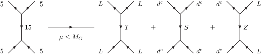
Figure 2: The $d=6$ supergraph from the $15$ exchange in the $SU(5)$ symmetric phase (left). In the $SU(5)$ broken phase ($\mu\leq M_{G}$), the latter splits into the remaining three supergraphes (right) which generate the $B-L$ invariant $d=6$ Kähler operators $(LL)({L}^{\dagger}{L}^{\dagger})$, $(d^{c}d^{c})(d^{c{\dagger}}d^{c{\dagger}})$ and $(d^{c}L)(d^{c{\dagger}}{L}^{\dagger})$ at low-energy.

As mentioned above, the $B-L$ conserving superpotential of Eq. (LABEL:su5) contains the $M_{5}$-term from which the $\mu$-parameter emerges in $W_{0}$. This mass parameter is not predicted by our model and will be determined through the requirement of EWSB (notice that the coupling $XH_{1}H_{2}$ is forbidden by $B-L$).

Also the coupling $\xi$ in Eq. (LABEL:su5) could include $24$-insertions, therefore allowing different masses for the $15$-components. For simplicity, we consider the minimal case which implies a common mass $M_{S}=M_{Z}=M_{T}=M_{15}$ at the GUT scale. The Yukawa-unification condition

$${\bf Y}_{S}={\bf Y}_{T}={\bf Y}_{Z}={\bf Y}_{15}\,,$$ (12)

can either hold or not at $M_{G}$, depending on the type and size of the $SU(5)$ breaking effects. In this respect, we can discuss the following two extreme scenarios:

(A)  Eq. (12) holds at the GUT scale. As a consequence, flavour violation is extended to all the couplings ${\bf Y}_{S}$, ${\bf Y}_{T}$ and ${\bf Y}_{Z}$, originating FV effects both in the lepton and quark sector. In this work we shall focus on this general case.

(B)  The states $S$ and $Z$ have negligible Yukawa couplings [Eq. (12) does not hold because of $SU(5)$ breaking]. In this case, FV is confined to the lepton sector since the couplings in ${\bf Y}_{T}$ are the only ones which exhibit a non-trivial flavour structure. We have already studied this scenario in Ref. [13].

Beneath the messenger scale $M_{T}$, the particle content of our model is that of the MSSM and so, the superpotential reduces to the sum of the MSSM terms in $W_{0}$ and the effective neutrino mass operator

$$W_{<M_{T}}=W_{0}+\frac{{\lambda}{\bf Y}_{T}}{2M_{T}}(LH_{2})(LH_{2}).$$ (13)

As mentioned above, the vev of $F_{X}$ induces the only tree-level SSB terms which, below the GUT scale, read ($B_{T}=B_{15}$ at $M_{G}$)

$$-{\cal L}^{>M_{T}}_{{\rm soft}}=B_{T}M_{T}(T\bar{T}+Z\bar{Z}+S\bar{S})+{\rm h.c.}\,.$$ (14)

Such terms remove the mass degeneracy between the scalar and fermionic messenger components. To avoid tachyonic scalar messengers we require that $\xi\langle F_{X}\rangle<M_{T}^{2}$ (or $B_{T}<M_{T}$). At the tree-level, the ordinary MSSM supermultiplets are degenerate as they do not couple to the superfield $X$. Nevertheless, in the presence of the bilinear terms given in Eq. (14), the mass splitting is radiatively generated at the scale $M_{T}$ through the gauge and Yukawa interactions between the messenger states $S,\,T$ and $Z$ and the ordinary MSSM fields. Our scenario can be, therefore, regarded as a gauge and Yukawa mediated SUSY breaking realization of the triplet seesaw mechanism. This will become clear in the next section where we present the complete MSSM SSB lagrangian.

4 The SSB mass parameters

We now discuss the SSB terms of the MSSM lagrangian ${\cal L}^{\rm MSSM}_{\rm soft}$ which are generated at the decoupling scale of the heavy states $S,T$ and $Z$. Below $M_{T}$, the most general ${\cal L}^{\rm MSSM}_{\rm soft}$ can be written as:

$$-{\cal L}^{\rm MSSM}_{\rm soft}\!\!\!\!\! = \!\!\!\!\!{\tilde{L}}^{\dagger}{\bf m}^{2}_{{\tilde{L}}}{\tilde{L}}+{\tilde{e^{c}}}{\bf m}^{2}_{{\tilde{e^{c}}}}{\tilde{e^{c}}}^{\dagger}+{\tilde{Q}}^{\dagger}{\bf m}^{2}_{{\tilde{Q}}}{\tilde{Q}}+{\tilde{d^{c}}}{\bf m}^{2}_{{\tilde{d^{c}}}}{\tilde{d^{c}}}^{\dagger}+{\tilde{u^{c}}}{\bf m}^{2}_{{\tilde{u^{c}}}}{\tilde{u^{c}}}^{\dagger}+m^{2}_{H_{1}}H^{\dagger}_{1}H_{1}+m^{2}_{H_{2}}H^{\dagger}_{2}H_{2}$$ (15)

$$+(H_{1}{\tilde{e^{c}}}{\bf A}_{e}{\tilde{L}}+H_{1}{\tilde{d^{c}}}{\bf A}_{d}{\tilde{Q}}+{\tilde{u^{c}}}{\bf A}_{u}{\tilde{Q}}H_{2}+\frac{1}{2}M_{a}{\lambda}_{a}{\lambda}_{a}+B_{H}\mu H_{2}H_{1}+{\mbox{h}.c.})\,,$$

where we have adopted the standard notation for the slepton, squark and Higgs soft masses, the trilinear couplings ${\bf A}_{e,d,u}$, the gaugino masses $M_{a}$ and the Higgs bilinear term $B_{H}$.

At the mass scale $M_{T}$, one-loop finite contributions are generated for ${\bf A}_{e,d,u}$, $M_{a}$ and $B_{H}$.

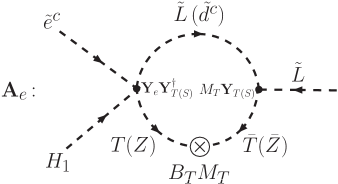
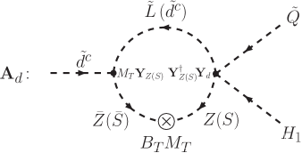
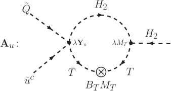
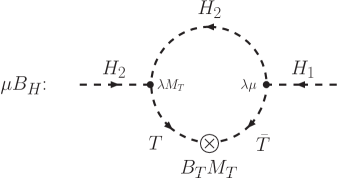
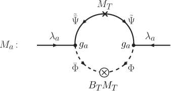
Figure 3: One-loop diagrams for the trilinear terms ${\rm A}_{e}$, ${\rm A}_{d}$ and ${\rm A}_{u}$ (first and second rows) and the bilinear Higgs term $\mu B_{H}$ and gaugino masses $M_{a}$ (third row). The fields $\Phi(\bar{\Phi})$ and $\tilde{\Psi}(\tilde{\bar{\Psi}})$ denote the scalar and fermionic components of the $T(\bar{T}),Z(\bar{Z}),S(\bar{S})$ superfields in such a way that $\Phi=(T,Z,S),(T,Z),(S,Z)$ and $\tilde{\Psi}=(\tilde{T},\tilde{Z},\tilde{S}),(\tilde{T},\tilde{Z}),(\tilde{S},\tilde{Z})$ for $a=1,2,3$, respectively (the assignments for $\bar{\Phi}$ and $\tilde{\bar{\Psi}}$ are obvious).

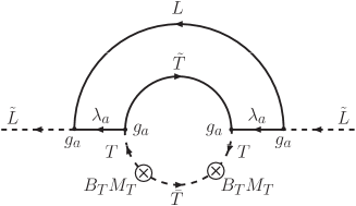
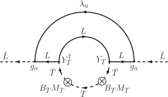
Figure 4: Examples of two-loop diagrams which contribute to ${\rm m}_{\tilde{L}}^{2}$. The upper diagrams generate contributions proportional to $g_{1,2}^{4}$ (left) and to $g_{1,2}^{2}{\rm Y}_{T}^{\dagger}{\rm Y}_{T}$ (right). Instead, the lower diagram leads to a term proportional $g_{a}^{2}{\bf Y}_{Z}^{\dagger}{\bf Y}_{Z}$.

In Fig. 3 we draw the one-loop diagrams for ${\bf A}_{e},{\bf A}_{d}$ and ${\bf A}_{u}$ (first and second rows), $\mu B_{H}$ and $M_{a}$ (third row). The evaluation of these diagrams yields:

$${{\bf A}}_{e} = \frac{3B_{T}}{16\pi^{2}}{\bf Y}_{e}({\bf Y}^{\dagger}_{T}{\bf Y}_{T}+{\bf Y}^{\dagger}_{Z}{\bf Y}_{Z})\,,$$

$${{\bf A}}_{u} = \frac{3B_{T}}{16\pi^{2}}|{\lambda}|^{2}{\bf Y}_{u}\,,$$

$${{\bf A}}_{d} = \frac{2B_{T}}{16\pi^{2}}({\bf Y}_{Z}{\bf Y}^{\dagger}_{Z}+2{\bf Y}_{S}{\bf Y}^{\dagger}_{S}){\bf Y}_{d}\,,$$

$$M_{a} = \frac{7B_{T}}{16\pi^{2}}\,g_{a}^{2}\,,$$

$$B_{H} = \frac{3B_{T}}{16\pi^{2}}\,|{\lambda}|^{2}.$$ (16)

In these expressions, $g_{a}(a=1,2,3)$ indicates the GUT normalized gauge coupling constants ($g_{1}=g_{2}=g_{3}$ at the unification scale) and the factor $N=7$ in the r.h.s. of the gaugino masses $M_{a}$ corresponds to twice the Dynkin index of the 15-representation. A noteworthy feature of the above equations is that both the $A$-terms and the Higgs doublet bilinear parameter $B_{H}$ are generated in our scenario, once the Yukawa couplings and the $\mu$ parameter are present in the superpotential.This is in contrast with the minimal GMSB realizations, where only the gaugino masses emerge at one-loop [27, 28]. We remark that the triplet states, being $SU(3)$ singlets, would not communicate SUSY breaking to the gluino. This is one more motivation, besides the aforementioned gauge coupling unification requirement, to consider the GUT extension of the triplet seesaw with the 15 representation.

Regarding the SSB squared scalar masses, the leading ${\cal O}(F^{2}_{X}/M^{2}_{T})={\cal O}(B^{2}_{T})$ contributions vanish at the one-loop level due to a cancelation among the different terms [29]. For example, in the case of the soft masses ${\bf m}^{2}_{{\tilde{L}}}$, the one-loop diagrams driven by the exchange of the $F$-component of $T$ cancel against those from the exchange of the $F$-component of $L$. Non-vanishing ${\cal O}(F^{2}_{X}/M^{2}_{T})$ contributions for the SSB squared scalar masses arise at the two-loop level. They are finite and can be evaluated either by diagrammatic computations or by means of a generalization of the wave function renormalization method proposed in Ref. [30, 31]. For the sake of illustration, we have depicted in Fig. 4 some representative two-loop diagrams which generate contributions to ${\bf m}^{2}_{\tilde{L}}$. The first diagram gives flavour-blind terms proportional to $g^{4}_{1,2}$. In turn, the remaining two diagrams generate LFV contributions proportional to $g^{2}_{1,2}{\bf Y}^{\dagger}_{T}{\bf Y}_{T}$ and to $g^{2}_{1,2,3}{\bf Y}^{\dagger}_{Z}{\bf Y}_{Z}$. In Appendix A we revisit the wave function renormalization approach and provide general formulas to extract all the SSB terms just by knowing the one-loop anomalous dimension matrices of the different fields above and below the messenger scale $M_{T}$. Our computation leads to the following result:

$$\!\!\!\!{\bf m}^{2}_{{\tilde{L}}} = \left(\frac{|B_{T}|}{16\pi^{2}}\right)^{2}\left[\frac{21}{10}g^{4}_{1}+\frac{21}{2}g^{4}_{2}-\left(\frac{27}{5}g^{2}_{1}+21g^{2}_{2}\right)\!{\bf Y}^{\dagger}_{T}{\bf Y}_{T}-\left(\frac{21}{15}g^{2}_{1}+9g^{2}_{2}+16g^{2}_{3}\right)\!{\bf Y}^{\dagger}_{Z}{\bf Y}_{Z}\right.$$

$$\!\left.+18({\bf Y}^{\dagger}_{T}{\bf Y}_{T})^{2}+15({\bf Y}^{\dagger}_{Z}{\bf Y}_{Z})^{2}+3{\rm Tr}({\bf Y}^{\dagger}_{T}{\bf Y}_{T}){\bf Y}^{\dagger}_{T}{\bf Y}_{T}+12{\bf Y}^{\dagger}_{Z}{\bf Y}_{S}{\bf Y}^{\dagger}_{S}{\bf Y}_{Z}\right.$$

$$\!\left.+3{\rm Tr}({\bf Y}^{\dagger}_{Z}{\bf Y}_{Z}){\bf Y}^{\dagger}_{Z}{\bf Y}_{Z}+9{\bf Y}^{\dagger}_{T}{\bf Y}^{T}_{Z}{\bf Y}^{*}_{Z}{\bf Y}_{T}+9({\bf Y}^{\dagger}_{T}{\bf Y}_{T}{\bf Y}^{\dagger}_{Z}{\bf Y}_{Z}+{\rm h.c.})\right.$$

$$\!\left.+3{\bf Y}^{\dagger}_{T}{\bf Y}^{T}_{e}{\bf Y}^{*}_{e}{\bf Y}_{T}+6{\bf Y}^{\dagger}_{Z}{\bf Y}_{d}{\bf Y}^{\dagger}_{d}{\bf Y}_{Z}\right]$$

$$\!\!{\bf m}^{2}_{{\tilde{e^{c}}}} = \left(\frac{|B_{T}|}{16\pi^{2}}\right)^{2}\left[\frac{42}{5}g^{4}_{1}-6{\bf Y}_{e}({\bf Y}^{\dagger}_{T}{\bf Y}_{T}+{\bf Y}^{\dagger}_{Z}{\bf Y}_{Z}){\bf Y}^{\dagger}_{e}\right]$$

$$\!\!{\bf m}^{2}_{{\tilde{Q}}} = \left(\frac{|B_{T}|}{16\pi^{2}}\right)^{2}\left[\frac{7}{30}g^{4}_{1}+\frac{21}{2}g^{4}_{2}+\frac{56}{3}g^{4}_{3}-2{\bf Y}^{\dagger}_{d}({\bf Y}_{Z}{\bf Y}^{\dagger}_{Z}+2{\bf Y}_{S}{\bf Y}^{\dagger}_{S}){\bf Y}_{d}-3|{\lambda}|^{2}{\bf Y}^{\dagger}_{u}{\bf Y}_{u}\right]$$

$$\!\!{\bf m}^{2}_{{\tilde{u^{c}}}} = \left(\frac{|B_{T}|}{16\pi^{2}}\right)^{2}\left[\frac{56}{15}g^{4}_{1}+\frac{56}{3}g^{4}_{3}-6|{\lambda}|^{2}{\bf Y}_{u}{\bf Y}^{\dagger}_{u}\right]$$

$$\!\!{\bf m}^{2}_{{\tilde{d^{c}}}} = \left(\frac{|B_{T}|}{16\pi^{2}}\right)^{2}\left[\frac{14}{15}g^{4}_{1}+\frac{56}{3}g^{4}_{3}-\left(\frac{16}{5}g^{2}_{1}+48g^{2}_{3}\right){\bf Y}_{S}{\bf Y}^{\dagger}_{S}-\left(\frac{14}{15}g^{2}_{1}+6g^{2}_{2}+\frac{32}{3}g^{2}_{3}\right){\bf Y}_{Z}{\bf Y}^{\dagger}_{Z}\right.$$

$$\!\left.+32({\bf Y}_{S}{\bf Y}^{\dagger}_{S})^{2}+4{\rm Tr}({\bf Y}_{S}{\bf Y}^{\dagger}_{S}){\bf Y}_{S}{\bf Y}^{\dagger}_{S}+8{\bf Y}_{S}{\bf Y}^{*}_{Z}{\bf Y}^{T}_{Z}{\bf Y}^{\dagger}_{S}+6{\bf Y}_{Z}{\bf Y}^{\dagger}_{T}{\bf Y}_{T}{\bf Y}^{\dagger}_{Z}\right.$$

$$\!\left.+8({\bf Y}_{S}{\bf Y}^{\dagger}_{S}{\bf Y}_{Z}{\bf Y}^{\dagger}_{Z}+{\rm h.c.})+10({\bf Y}_{Z}{\bf Y}^{\dagger}_{Z})^{2}+2{\rm Tr}({\bf Y}_{Z}{\bf Y}^{\dagger}_{Z}){\bf Y}_{Z}{\bf Y}^{\dagger}_{Z}\right.$$

$$\!\left.+8{\bf Y}_{S}{\bf Y}_{d}^{*}{\bf Y}^{T}_{d}{\bf Y}^{\dagger}_{S}+2{\bf Y}_{Z}{\bf Y}_{e}^{\dagger}{\bf Y}_{e}{\bf Y}^{\dagger}_{Z}\right]$$

$$\!\!m^{2}_{H_{1}} = \left(\frac{|B_{T}|}{16\pi^{2}}\right)^{2}\left[\frac{21}{10}g^{4}_{1}+\frac{21}{2}g^{4}_{2}-3{\rm Tr}[({\bf Y}^{\dagger}_{T}{\bf Y}_{T}+{\bf Y}^{\dagger}_{Z}{\bf Y}_{Z}){\bf Y}^{\dagger}_{e}{\bf Y}_{e}]\right.$$

$$\!\left.-6{\rm Tr}[({\bf Y}_{Z}{\bf Y}^{\dagger}_{Z}+2{\bf Y}^{\dagger}_{S}{\bf Y}_{S}){\bf Y}^{\dagger}_{d}{\bf Y}_{d}]\right]$$

$$\!\!m^{2}_{H_{2}} = \left(\frac{|B_{T}|}{16\pi^{2}}\right)^{2}\left[\frac{21}{10}g^{4}_{1}+\frac{21}{2}g^{4}_{2}-\left(\frac{27}{5}g^{2}_{1}+21g^{2}_{2}\right)|{\lambda}|^{2}+9|{\lambda}|^{2}{\rm Tr}({\bf Y}_{u}{\bf Y}^{\dagger}_{u})+21|{\lambda}|^{4}\right].$$ (17)

One can immediately recognize that the diagonal gauge-mediated contributions follow the expected form $\propto 2k_{a}C^{f}_{a}Ng^{4}_{a}\,(k_{1}=3/5,k_{2}=k_{3}=1)$, where $C^{f}_{a}$ is the quadratic Casimir of the $f$-particle [$C^{f}_{1}=Y^{2}_{f}=(Q_{f}-T^{3}_{f})^{2}$ and $C=\frac{n^{2}-1}{2n}$ for the fundamental representation of $SU(n)$].

The above expressions hold at the decoupling scale $M_{T}$ and are, therefore, meant as boundary conditions for the SSB parameters which then undergo (MSSM) RG running down to the low-energy scale $\mu_{s}$. All the soft masses have the same scaling property $m_{soft}\sim B_{T}/(16\pi^{2})$ which, on the basis of the naturalness requirement $m_{soft}\sim{\cal O}(10^{2}-10^{3}~{}{\rm GeV})$, implies that $B_{T}\lower 3.01385pt\hbox{$\;\stackrel{{\scriptstyle\textstyle>}}{{\sim}}\;$}10~{}{\rm TeV}$. In principle, the SSB parameters also receive gravity mediated contributions of order the gravitino mass $m_{3/2}\sim F/M_{PL}$ ($F^{2}=\langle|F_{X}|^{2}\rangle+\ldots$ is the sum of $F$-terms in the secluded sector). We assume such contributions to be negligible, which is the case if $M_{T}\ll~{}10^{16}~{}{\rm GeV}\,\xi\langle F_{X}\rangle/F$. This also implies that the gravitino is lighter than the MSSM sparticles.

It is apparent from Eqs. (16) and (4) (and Figs. 3 and 4) that the gauge interactions participate in the mediation of SUSY breaking in the gaugino and soft scalar masses. In the particular case of the sfermion mass matrices, the associated terms constitute the flavour blind contribution. Exactly the same situation occurs in pure GMSB models where flavour violation is automatically suppressed if the SUSY-breaking mediation scale is lower than the flavour or GUT scale [27, 28, 32]. In our case, SUSY breaking is also mediated by the Yukawa interactions ${\bf Y}_{S},{\bf Y}_{T},{\bf Y}_{Z}$ and ${\lambda}$, giving rise to the bilinear parameter $B_{H}$, the trilinear couplings ${\bf A}_{e,d,u}$ and to additional contributions to the Higgs scalar masses and the sfermion mass matrices. In this way, FV is transmitted to the SSB mass parameters. Since the origin of FV originally comes from the couplings ${\bf Y}_{15}$ (felt by the $\bar{5}$ supermultiplets), one expects that, due to the condition (12), flavour violation is inherited with comparable size by the ${\tilde{L}}$ and ${\tilde{d^{c}}}$ SSB parameters ${\bf A}_{e}$,${\bf A}_{d}$, ${\bf m}^{2}_{{\tilde{L}}}$ and ${\bf m}^{2}_{{\tilde{d^{c}}}}$. We emphasize that the FV entries of e.g., $({\bf m}^{2}_{\tilde{L}})_{ij}$ $(i\neq j)$ show up as finite radiative contributions induced by $B_{T}$ at $M_{T}$, and they are not significantly modified by the running evolution to low-energy. This is different from a previous work [9] where a common SSB scalar mass $m_{0}\sim{\cal O}(100~{}{\rm GeV})$ was assumed at $M_{G}$ and the dominant LFV contributions to ${\bf m}^{2}_{\tilde{L}}$ were generated by RG evolution from $M_{G}$ down to the decoupling scale $M_{T}$ [see Eq. (6)]. In such a case, finite contributions like those in Eqs. (16) and (4) also emerge at $M_{T}$. Nevertheless, they are subleading with respect to the RG corrections, since $B_{T}$ is of the same order as $m_{0}$. Instead, in the present picture, there is a hierarchy between the SSB parameter $B_{T}$ and the remaining ones [see Eqs. (16) and (4)], $B^{2}_{T}\gg(B_{T}g^{2}/16\pi^{2})^{2}\sim m^{2}_{0}$ [13].

5 Flavour structure in ${\bf m}^{2}_{\tilde{L}}$ and ${\bf m}^{2}_{\tilde{d^{c}}}$ from neutrino parameters

In this section we discuss in detail the features of the flavour structure which emerges in the mass matrices ${\bf m}^{2}_{\tilde{L}}$ and ${\bf m}^{2}_{\tilde{d^{c}}}$, and in the trilinear couplings ${\bf A}_{e}$ and ${\bf A}_{d}$. These parameters depend on the Yukawa couplings ${\bf Y}_{T},{\bf Y}_{S},{\bf Y}_{Z}$. The matrix ${\bf Y}_{T}$ is determined at $M_{T}$ according to the matching expressed by Eq. (3) i.e.,

$${\bf Y}_{T}=\frac{M_{T}}{{\lambda}v^{2}_{2}}\,{\bf m}_{\nu}\,,$$ (18)

where the effective neutrino mass matrix ${\bf m}_{\nu}$ has undergone the MSSM RG running from low-energy to $M_{T}$. The matrices ${\bf Y}_{S}$ and ${\bf Y}_{Z}$ are iteratively determined at $M_{T}$ under the unification constraint of Eq. (12). For the determination of the mass matrix ${\bf m}_{\nu}$ at low-energy [cf. Eq. (4)] we consider three different types of neutrino spectra:

1. Normal hierarchy (NH): $m_{1}\ll m_{2}<m_{3}$, with

   $$m^{2}_{2}=m^{2}_{1}+\Delta m^{2}_{S},~{}~{}~{}m^{2}_{3}=m^{2}_{1}+\Delta m^{2}_{S}+\Delta m^{2}_{A}\,,$$ (19)

2. Inverted hierarchy (IH): $m_{3}\ll m_{1}<m_{2}$, with

   $$m^{2}_{1}=m^{2}_{3}-\Delta m^{2}_{S}+\Delta m^{2}_{A},~{}~{}~{}m^{2}_{2}=m^{2}_{3}+\Delta m^{2}_{A}\,,$$ (20)

3. Quasi degenerate (QD): $m_{1}\approx m_{2}\approx m_{3}$, with

   $$m^{2}_{2}=m^{2}_{1}+\Delta m^{2}_{S},~{}~{}~{}m^{2}_{3}=m^{2}_{1}+\Delta m^{2}_{S}+\Delta m^{2}_{A},~{}~{}~{}m^{2}_{1}\gg\Delta m^{2}_{A}\,.$$ (21)

The neutrino mass squared differences $\Delta m^{2}_{A}=|m^{2}_{3}-m^{2}_{2}|$ and $\Delta m^{2}_{S}=m^{2}_{2}-m^{2}_{1}$ are responsible for the atmospheric and solar neutrino oscillations, respectively, together with the corresponding mixing angles $\theta_{23}$ and $\theta_{12}$ of the mixing matrix ${\bf V}$ [see Eq. (2)]. From global analysis of the neutrino oscillation data, the following best fit values are available (with their allowed $3\sigma$ range) [34]:

$$\Delta m^{2}_{A} = 2.2^{+1.1}_{-0.8}\times 10^{-3}~{}{\rm eV}^{2}\,\,\,,\,\,\,\sin^{2}\theta_{23}=0.5^{+0.18}_{-0.16}$$

$$\Delta m^{2}_{S} = 7.9^{+1.0}_{-0.8}\times 10^{-5}~{}{\rm eV}^{2},\,\,\,,\,\,\,\sin^{2}\theta_{12}=0.3^{+0.1}_{-0.6}$$ (22)

For the lepton mixing angle $\theta_{13}$ the following upper bound has been settled (at $3\sigma$) [34]:

$$\sin^{2}\theta_{13}<0.043\,.$$ (23)

It is worth noticing that, for a NH spectrum, the largest entries of ${\bf m}_{\nu}$ (and, hence, of ${\bf Y}_{T}$) are those in the $\tau-\mu$ block, where the largest neutrino mass $(\Delta m_{A}^{2})^{1/2}$ dominates. Moreover, they are of comparable size due to maximal atmospheric mixing. On the other hand, the remaining matrix elements are smaller by one or two orders of magnitude, depending on the value of $\theta_{13}$ (which introduces the dependence on $(\Delta m_{A}^{2})^{1/2}$ to these entries). In the IH case, while $({\bf m}_{\nu})_{ee}$ and the $\tau-\mu$ block are of the same order, $({\bf m}_{\nu})_{\mu e}$ and $({\bf m}_{\nu})_{\tau e}$ are generically smaller. Finally, when the neutrino mass spectrum is of the QD type, the leading mass $m_{1}$ renders the matrix pattern less hierarchical and enhances the overall magnitude of ${\bf m}_{\nu}$ (or, equivalently, of ${\bf Y}_{T}$).

Let us now turn to the flavour structure of the SSB parameters which are generated at the messenger scale $M_{T}$. For simplicity of our discussion, we temporarily assume that the unification condition (12) remains approximately valid at $M_{T}$, ${\bf Y}_{T}\approx{\bf Y}_{S}\approx{\bf Y}_{Z}$. In addition, we disregard the terms proportional to the Yukawa couplings ${\bf Y}_{e,d}$ in the expressions of ${\bf m}^{2}_{\tilde{L}}$ and ${\bf m}^{2}_{\tilde{d^{c}}}$ given in Eqs. (4). Under these assumptions, we can write:

$$({\bf m}^{2}_{\tilde{L}})_{ij} \!\!\approx\!\! -\left(\frac{{B_{T}}}{16\pi^{2}}\right)^{2}\kappa\left[{\bf V}({\bf m}^{D}_{\nu})^{2}{\bf V}^{\dagger}\right]_{ik}\left[c^{e}_{a}\,g^{2}_{a}\delta_{kj}-72\,\kappa\left[{\bf V}({\bf m}^{D}_{\nu})^{2}{\bf V}^{\dagger}\right]_{kj}-6\,\kappa{\rm Tr}({\bf m}^{D}_{\nu})^{2}\delta_{kj}\right],$$

$$({\bf A}_{e})_{ij} \approx \frac{{3B_{T}}}{8\pi^{2}}\,\kappa\,({\bf Y}_{e})_{ii}\left[{\bf V}({\bf m}^{D}_{\nu})^{2}{\bf V}^{\dagger}\right]_{ij},$$

$$({\bf m}^{2}_{\tilde{d^{c}}})^{*}_{ij} \!\!\approx\!\! -\left(\frac{{B_{T}}}{16\pi^{2}}\right)^{2}\kappa\left[{\bf V}({\bf m}^{D}_{\nu})^{2}{\bf V}^{\dagger}\right]_{ik}\left[c^{d}_{a}\,g^{2}_{a}\delta_{kj}-72\,\kappa\left[{\bf V}({\bf m}^{D}_{\nu})^{2}{\bf V}^{\dagger}\right]_{kj}-6\,\kappa{\rm Tr}({\bf m}^{D}_{\nu})^{2}\delta_{kj}\right],$$

$$({\bf A}_{d})^{*}_{ij} \approx \frac{{3B_{T}}}{8\pi^{2}}\kappa\left[{\bf V}({\bf m}^{D}_{\nu})^{2}{\bf V}^{\dagger}\right]_{ij}({\bf Y}_{d})_{jj}\quad\quad,\quad\quad\kappa=\left(\frac{M_{T}}{{\lambda}v^{2}_{2}}\right)^{\!2}\,,$$ (24)

where $c^{e}_{a},c^{d}_{a}$ are: $c^{e}_{1}=\frac{102}{15}\,,c^{e}_{2}=30\,,c^{e}_{3}=16$, $c^{d}_{1}=\frac{62}{15}~{},c^{d}_{2}=6$ and $c^{d}_{3}=\frac{176}{3}$ (summation of repeated indices is implicit). The flavour indices are $i,j=e,\mu,\tau\,(d,s,b)$ for the slepton (squark) matrices ${\bf m}^{2}_{\tilde{L}}$ and ${\bf A}_{e}$ (${\bf m}^{2}_{\tilde{d^{c}}}$ and ${\bf A}_{d}$). Wherever necessary, the correspondences $e\leftrightarrow d,\mu\leftrightarrow s,\tau\leftrightarrow b$ are understood.

From Eqs. (3)-(2), and considering the three different kinds of neutrino mass spectra shown in (19)-(21), we have:

$$\left[{\bf V}({\bf m}^{D}_{\nu})^{2}{\bf V}^{\dagger}\right]_{ij}=\left\{\begin{array}[]{l}m^{2}_{1}\delta_{ij}+\Delta m^{2}_{S}{\bf V}_{i2}{\bf V}^{*}_{j2}+(\Delta m^{2}_{A}+\Delta m^{2}_{S}){\bf V}_{i3}{\bf V}^{*}_{j3}\;\;\;{\rm(NH,QD)}\\ \\ m^{2}_{3}\delta_{ij}+\Delta m^{2}_{A}{\bf V}_{i2}{\bf V}^{*}_{j2}+(\Delta m^{2}_{A}-\Delta m^{2}_{S}){\bf V}_{i1}{\bf V}^{*}_{j1}\;\;\;{\rm(IH)}\end{array}\right.\,,$$ (28)

which manifestly shows that the FV ($i\neq j$) entries are always independent of the lightest neutrino mass. The explicit expressions in terms of the neutrino parameters read:

$$\left[{\bf V}({\bf m}^{D}_{\nu})^{2}{\bf V}^{\dagger}\right]_{\tau\mu} = \pm{\Delta m^{2}_{A}}\left[c^{2}_{13}c_{23}s_{23}\pm\rho\,\left(c_{23}s_{23}(s^{2}_{12}-c^{2}_{12}s^{2}_{13})+c_{12}s_{12}s_{13}(s^{2}_{23}-c^{2}_{23})\right)\right]$$

$$\left[{\bf V}({\bf m}^{D}_{\nu})^{2}{\bf V}^{\dagger}\right]_{\mu e} = \pm\Delta m^{2}_{A}c_{13}\left[s_{13}s_{23}\pm\rho\,c_{12}\left(c_{23}s_{12}+c_{12}s_{23}s_{13}\right)\right]\,$$

$$\left[{\bf V}({\bf m}^{D}_{\nu})^{2}{\bf V}^{\dagger}\right]_{\tau e} = \pm{\Delta m^{2}_{A}}c_{13}\left[c_{23}s_{13}\mp\rho\,c_{12}\left(s_{23}s_{12}-c_{12}c_{23}s_{13}\right)\right]\,,$$ (29)

where the upper (lower) sign applies for either the NH or QD (IH) neutrino spectrum, and $\rho=\Delta m^{2}_{S}/\Delta m^{2}_{A}\approx 0.04$. Due to the smallness of the parameter $\rho$, the quantities $|({\bf Y}^{\dagger}_{T}{\bf Y}_{T})_{ij}|\propto|[{\bf V}({\bf m}^{D}_{\nu})^{2}{\bf V}^{\dagger}]_{ij}|$ are not sensitive to the type of neutrino mass spectrum, unless $s_{13}\approx\rho\,c_{12}s_{12}c_{23}/c_{23}\,({\rm or}\,\rho\,c_{12}s_{12}c_{23}/s_{23})\approx 0.02$. For such values of $s_{13}$, the $\mu e$ and $sd$ ($\tau e$ and $bd$) matrix elements in Eqs. (5) would be strongly suppressed or even vanish for a IH (NH) mass pattern. Instead, the entries $\tau\mu\,(bs)$ do not change significantly with $\theta_{13}$, since the terms proportional to $s_{13}$ are suppressed by $\rho\cos(2\theta_{23})\approx 0$. The quartic combinations $\left[{\bf V}({\bf m}^{D}_{\nu})^{2}{\bf V}^{\dagger}\right]^{2}$ can be approximately obtained from the corresponding quadratic ones of Eq. (5) by performing the following replacements:

$${\rm NH} \!\!\!\!\!\!\!\!:\,\,\Delta m^{2}_{A}\rightarrow(\Delta m^{2}_{A})^{2}(1+2\rho)\;\;\quad,\quad\;\;\rho\rightarrow\rho^{2}(1-2\rho)\,,$$

$${\rm\vskip 6.0pt plus 2.0pt minus 2.0pt}{\rm IH} \!\!\!\!\!\!\!\!:\,\,\Delta m^{2}_{A}\rightarrow(\Delta m^{2}_{A})^{2}\;\;\quad\quad\quad\;\;\quad,\quad\;\;\rho\longrightarrow 2\rho\left(1-\frac{\rho}{2}\right)\,,$$

$${\rm QD} \!\!\!\!\!\!\!\!:\,\,\Delta m^{2}_{A}\longrightarrow 2\,m^{2}_{1}\,\Delta m^{2}_{A}\;\;\quad\quad\;\;\,\;,\quad\;\;\rho\rightarrow\rho\,.$$ (30)

It is then straightforward to obtain the explicit expressions for the r.h.s. of Eqs. (5), taking into account Eqs. (5) and (5). However, it is more instructive to consider the results for certain ranges of $\theta_{13}$. Let us focus on ${\bf m}^{2}_{\tilde{L}}$, as the result for ${\bf m}^{2}_{\tilde{d^{c}}}$ will follow directly. Distinguishing the three types of neutrino mass neutrino spectra, we find:

$\bullet\,$ NH spectrum, for $s_{13}\ll\rho^{2}c_{23}c_{12}s_{12}/s_{23}\approx 8\times 10^{-4}$:

$$({\bf m}^{2}_{{\tilde{L}}})_{\tau\mu} \!\!\!\approx\!\!\! -\left(\frac{B_{T}}{16\pi^{2}}\right)^{2}\kappa\,\left[{\bf V}({\bf m}^{D}_{\nu})^{2}{\bf V}^{\dagger}\right]_{\tau\mu}\,\left[c^{e}_{a}g^{2}_{a}-78\,\kappa\Delta m^{2}_{A}(1+2\rho)\right],$$

$$({\bf m}^{2}_{{\tilde{L}}})_{\mu e,\tau e} \!\!\!\approx\!\!\! -\left(\frac{B_{T}}{16\pi^{2}}\right)^{2}\kappa\,\left[{\bf V}({\bf m}^{D}_{\nu})^{2}{\bf V}^{\dagger}\right]_{\mu e,\tau e}\,\left[c^{e}_{a}g^{2}_{a}-6\,\kappa\Delta m^{2}_{A}(1+14\rho)\right]\,,$$ (31)

while for $s_{13}\gg\rho c_{23}c_{12}s_{12}/s_{23}\approx 0.02$:

$$({\bf m}^{2}_{\tilde{L}})_{ij}\approx-\left(\frac{{B_{T}}}{16\pi^{2}}\right)^{2}\kappa\,\left[{\bf V}({\bf m}^{D}_{\nu})^{2}{\bf V}^{\dagger}\right]_{ij}\,\left[c^{e}_{a}g^{2}_{a}-78\,\kappa\Delta m^{2}_{A}(1+2\rho)\right]$$ (32)

$\bullet\,$ IH spectrum for $s_{13}\ll\rho c_{23}c_{12}s_{12}/s_{23}\approx 0.02$:

$$({\bf m}^{2}_{{\tilde{L}}})_{\tau\mu} \!\!\!\approx\!\!\! -\left(\frac{B_{T}}{16\pi^{2}}\right)^{2}\kappa\,\left[{\bf V}({\bf m}^{D}_{\nu})^{2}{\bf V}^{\dagger}\right]_{\tau\mu}\,\left(c^{e}_{a}g^{2}_{a}-84\,\kappa\Delta m^{2}_{A}\right),$$

$$({\bf m}^{2}_{{\tilde{L}}})_{\mu e,\tau e} \!\!\!\approx\!\!\! -\left(\frac{B_{T}}{16\pi^{2}}\right)^{2}\kappa\,\left[{\bf V}({\bf m}^{D}_{\nu})^{2}{\bf V}^{\dagger}\right]_{\mu e\,\tau e}\,\left(c^{e}_{a}g^{2}_{a}-156\,\kappa\Delta m^{2}_{A}\right),$$

while for $s_{13}\gg 2\rho c_{23}c_{12}s_{12}/s_{23}\approx 0.04$:

$$({\bf m}^{2}_{\tilde{L}})_{ij}\approx-\left(\frac{{B_{T}}}{16\pi^{2}}\right)^{2}\kappa\,\left[{\bf V}({\bf m}^{D}_{\nu})^{2}{\bf V}^{\dagger}\right]_{ij}\,\left(c^{e}_{a}g^{2}_{a}-84\,\kappa\Delta m^{2}_{A}\right).$$ (34)

$\bullet\,$ QD spectrum (for any value of $s_{13}$)

$$({\bf m}^{2}_{\tilde{L}})_{ij}\approx-\left(\frac{{B_{T}}}{16\pi^{2}}\right)^{2}\kappa\,\left[{\bf V}({\bf m}^{D}_{\nu})^{2}{\bf V}^{\dagger}\right]_{ij}\left[c^{e}_{a}g^{2}_{a}-162\,\kappa\,m^{2}_{1}\left(1+\frac{\Delta m^{2}_{A}}{27m^{2}_{1}}\right)\right].$$ (35)

The above expressions exhibit the relevant flavour violating factors $[{\bf V}(m^{D}_{\nu})^{2}{\bf V}^{\dagger}]_{ij}$ separated from the piece composed by terms proportional to the gauge couplings $g_{a}^{2}$ and terms proportional to $\kappa\,\Delta m^{2}_{A}$ (NH and IH) or $\kappa\,m^{2}_{1}$ (QD). For a given effective SUSY breaking scale $B_{T}$, the overall size of those entries is controlled by $\kappa\propto(M_{T}/{\lambda})^{2}$. It is interesting to notice that, for a certain value of $M_{T}/{\lambda}$, the $g_{a}^{2}$-terms are canceled and thus all the three off-diagonal entries can be vanishing. If $s_{13}\gg 0.02$, this peculiar flavour-blind suppression happens when $M_{T}/{\lambda}\sim v^{2}_{2}(\frac{c^{e}_{a}g^{2}_{a}}{78\Delta m^{2}_{A}})^{1/2}$ and $M_{T}/{\lambda}\sim v^{2}_{2}(\frac{c^{e}_{a}g^{2}_{a}}{84\Delta m^{2}_{A}})^{1/2}$, for the NH and IH neutrino spectrum, respectively. Instead, for the QD case, the suppression occurs for $M_{T}/{\lambda}\sim v^{2}_{2}(\frac{c^{e}_{a}g^{2}_{a}}{162m^{2}_{1}})^{1/2}$, irrespective of $s_{13}$. If $s_{13}$ is tiny and the neutrino spectrum is either NH or IH, the entry $(\tau\mu)$ is suppressed for $M_{T}/{\lambda}$ smaller (larger) by $\approx 1/3$ ($\approx 1.4$), with respect to the entry $(\mu e)$ [$(\tau e)$] for the NH (IH) spectrum. We can summarise this analysis saying that the off-diagonal entries of ${\bf m}^{2}_{\tilde{L}}$ and ${\bf m}^{2}_{\tilde{d^{c}}}$ can undergo a strong reduction in two cases: 1) when $s_{13}\approx 0.02$ and so the quantities $[{\bf V}({\bf m}^{D}_{\nu})^{2}{\bf V}^{\dagger}]_{\tau e}$ and $[{\bf V}({\bf m}^{D}_{\nu})^{2}{\bf V}^{\dagger}]_{\mu e}$ are vanishing for the NH and IH spectrum, respectively; 2) when there is a cancelation between the quadratic and quartic contributions, which depends on the parameters $M_{T}$ and ${\lambda}$ and on the neutrino spectrum.

In the parameter range where the FV entries $({\bf m}^{2}_{\tilde{L}})_{ij}$ are dominated by either the quadratic or the quartic Yukawa terms, the relative size of LFV (QFV) in the $\mu-\tau$ ($b-s$) and $\mu-e$ ($s-d$) sectors, does not depend of the ratio $M_{T}/{\lambda}$, and can be approximately predicted in terms of only the low-energy observables ${\bf V}$ and ${\bf m}^{D}_{\nu}$, as:

$$R_{23/12}=\frac{({\bf m}^{2}_{\tilde{L}})_{\tau\mu}}{({\bf m}^{2}_{\tilde{L}})_{\mu e}}\sim\frac{({\bf m}^{2}_{{\tilde{d^{c}}}})_{bs}}{({\bf m}^{2}_{{\tilde{d^{c}}}})_{sd}} \approx \frac{\left[{\bf V}({\bf m}^{D}_{\nu})^{2}{\bf V}^{\dagger}\right]_{\tau\mu}}{\left[{\bf V}({\bf m}^{D}_{\nu})^{2}{\bf V}^{\dagger}\right]_{\mu e}},$$

$$R_{13/12}=\frac{({\bf m}^{2}_{\tilde{L}})_{\tau e}}{({\bf m}^{2}_{\tilde{L}})_{\mu e}}\sim\frac{({\bf m}^{2}_{{\tilde{d^{c}}}})_{bd}}{({\bf m}^{2}_{{\tilde{d^{c}}}})_{sd}} \approx \frac{\left[{\bf V}({\bf m}^{D}_{\nu})^{2}{\bf V}^{\dagger}\right]_{\tau e}}{\left[{\bf V}({\bf m}^{D}_{\nu})^{2}{\bf V}^{\dagger}\right]_{\mu e}}\,.$$ (36)

Plugging the results of Eqs. (5) into the above expressions, and taking the central values (5) for the neutrino parameters, we have:

$$R_{23/12}|_{s_{13}=0} \approx 40\,(-40),\,\,\,\,\,\,\,\,\,\,~{}~{}~{}~{}~{}R_{23/12}|_{s_{13}=0.2}\approx 3.2\,(3.8),$$

$$R_{13/12}|_{s_{13}=0} \approx -1\,(-1)\,\,\,\,~{}~{}~{}~{}~{}~{}~{}~{}~{}~{}R_{13/12}|_{s_{13}=0.2}\approx 0.8\,(1.2)\,,$$ (37)

for the NH (IH) spectrum. The QD case gives the same results as the NH one.

6 Phenomenological viability

In the previous sections, we have set up a theoretical framework consisting of the superpotential (13) and the SSB lagrangian (15), beneath the energy scale $M_{T}$, whose relevant soft mass parameters (16, 4) emerge at the messenger energy scale. Next, we describe the criteria employed to constrain the parameter space spanned by $M_{T},B_{T}$ and ${\lambda}$. With the purpose of investigating the phenomenological viability of our scenario, a detailed numerical analysis is carried out in Section 6.2. The results are then thoroughly discussed.

6.1 The phenomenological constraints

Our approach to relate the low-energy measured parameters with the high-energy quantities, such as the Yukawa couplings, follows a bottom-up perspective. In particular, this allows us to determine the following quantities:

• The matrix ${\bf Y}_{T}$ (as well as ${\bf Y}_{S}$ and ${\bf Y}_{Z}$) is determined at $M_{T}$ as already explained in the previous section [see Eq. (18)].

• The Yukawa matrices ${\bf Y}_{e},{\bf Y}_{u},{\bf Y}_{d}$ are extracted from the corresponding charged fermion masses, modulo $\tan\beta$.

• The remaining low-energy input parameters $\mu(\mu_{s})$ (with its sign) and $\tan\beta$ are determined by the EWSB conditions:

  $$\mu^{2}=\frac{-\tan^{2}\beta\overline{m}^{2}_{H_{2}}+\overline{m}^{2}_{H_{1}}}{\tan^{2}\beta-1}-\frac{M^{2}_{Z}}{2}\;\quad\quad,\quad\quad\;\sin 2\beta=\frac{2\mu B_{H}}{\overline{m}^{2}_{H_{1}}+\overline{m}^{2}_{H_{2}}+2\mu^{2}}\,.$$ (38)

  We have included the one-loop tadpole corrections $t_{1,2}$ through the redefinition of the Higgs scalar masses, i.e. $\overline{m}^{2}_{H_{1}}={m}^{2}_{H_{1}}-\frac{t_{1}}{\sqrt{2}v\cos\beta},\overline{m}^{2}_{H_{2}}={m}^{2}_{H_{2}}-\frac{t_{2}}{\sqrt{2}v\sin\beta}$. According to the standard practice, the above minimisation conditions are imposed at the scale $\mu_{s}=\sqrt{m_{\tilde{t}_{1}}m_{\tilde{t}_{2}}}$.

Hence, we are left with three free parameters, $M_{T},B_{T}$ and the coupling ${\lambda}$, which can all be taken to be real, without loss of generality.

BR	Present limits	Future sensitivity
$\mu^{-}\to e^{-}\gamma$	$1.2\times 10^{-11}$ [35]	$10^{-14}$ [36]
$\tau^{-}\to\mu^{-}\gamma$	$6.8\times 10^{-8}$ [37]	$10^{-9}~{}\cite[cite]{[\@@bibref{}{taumu:fut}{}{}]}$
$\tau^{-}\to e^{-}\gamma$	$1.1\times 10^{-7}$ [39]	$10^{-9}~{}\cite[cite]{[\@@bibref{}{taumu:fut}{}{}]}$
$\mu^{-}\to e^{-}e^{+}e^{-}$	$1.0\times 10^{-12}$ [40]	$10^{-14}$ [41]
$\tau^{-}\to\mu^{-}\mu^{+}\mu^{-}$	$1.9\times 10^{-7}$ [42]	$10^{-9}~{}\cite[cite]{[\@@bibref{}{taumu:fut}{}{}]}$
$\tau^{-}\to\mu^{-}e^{+}e^{-}$	$1.9\times 10^{-7}$ [43]	$10^{-9}~{}\cite[cite]{[\@@bibref{}{taumu:fut}{}{}]}$
$\tau^{-}\to e^{-}e^{+}e^{-}$	$2.0\times 10^{-7}$ [44]	$10^{-9}~{}\cite[cite]{[\@@bibref{}{taumu:fut}{}{}]}$
$\tau^{-}\to e^{-}\mu^{+}\mu^{-}$	$3.3\times 10^{-7}$ [44]	$10^{-9}~{}\cite[cite]{[\@@bibref{}{taumu:fut}{}{}]}$
CR($\mu\to e\,$; Ti )	$1.7\times 10^{-12}$ [45]	$10^{-18}~{}\cite[cite]{[\@@bibref{}{prime}{}{}]}$

Table 1: Present limits and future sensitivities for the branching ratios (BR) of several LFV processes. The bound on the $\mu\to e$ conversion rate (CR) in Ti is also shown.

The parameter space spanned by these parameters is constrained as follows.

• We impose the constraint coming from the decay $\mu\to e\gamma$, using the results in [11]. The experimental upper bound for the branching ratio of this decay is shown in Table 1. The relevant LFV entry is $({\bf m}^{2}_{\tilde{L}})_{\mu e}$ [see Eqs. (5) and (5)].

• A conservative limit upon the lightest Higgs boson mass, $m_{h}>110~{}{\rm GeV}$, is considered on the basis of the negative LEP2 direct searches [47]. Our predictions on $m_{h}$ include the low-energy radiative corrections which are obtained linking our code to FeynHiggs [48].

• We also require that the sparticle masses (which pass the tachyonic test) respect the experimental lower bounds set by Tevatron and LEP direct searches [15].

• The SUSY contribution to the anomalous magnetic moment of the muon $\delta a_{\mu}$ [11] has been considered and subjected to the following constraint at $99\%\,$ C.L. [49]:

  $$-13\times 10^{-10}<\delta a_{\mu}<57\times 10^{-10}\,.$$ (39)

  However, we will see that this requirement does not imply an important constraint on the parameter space.

• We have checked that all the coupling constants remain in the perturbative regime up to the scale $M_{G}$. In particular, while the presence of a complete GUT representation below $M_{G}$ does not alter the value of $M_{G}$, the gauge coupling $g_{G}$ gets an additional contribution $\delta g^{-2}_{G}=\frac{N}{8\pi}{\rm ln}({M_{T}}/{M_{G}})$. The requirement of perturbativity implies $\frac{N}{2\pi}{\rm ln}({M_{G}}/{M_{T}})\lower 3.01385pt\hbox{$\;\stackrel{{\scriptstyle\textstyle<}}{{\sim}}\;$}24$ which, for $N=7$, gives $M_{T}\lower 3.01385pt\hbox{$\;\stackrel{{\scriptstyle\textstyle>}}{{\sim}}\;$}10^{7}~{}{\rm GeV}$. The parameter space is further restricted by imposing the perturbativity requirement on the coupling constants ${\lambda}$, ${\bf Y}_{T},{\bf Y}_{S}$ and ${\bf Y}_{Z}$.

As it will be shown in the next section, the most stringent constraints come from the sparticle spectrum, $\mu\to e\gamma$ decay, the Higgs boson mass and the requirement of radiative EWSB and perturbativity.

6.2 Parameter space analysis

In Fig. 5 the constraints imposed on the parameter space $({\lambda},M_{T})$ are shown for $B_{T}=20~{}{\rm TeV}$ and $s_{13}=0(0.2)$ in the upper (lower) panel, taking the NH neutrino spectrum (later we will comment on the other cases). The light-grey regions are excluded by the perturbativity requirement. For each value of $M_{T}$, there is a minimum value of ${\lambda}$, scaling as $\sim 2\times 10^{-4}(M_{T}/10^{11}~{}{\rm GeV})$, below which the couplings ${\bf Y}_{T}$ and/or ${\bf Y}_{S,Z}$ reach the Landau pole between $M_{T}$ and $M_{G}$. Similarly, there is an upper bound for ${\lambda}$, above which ${\lambda}$ itself blows up.

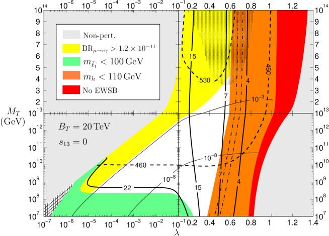
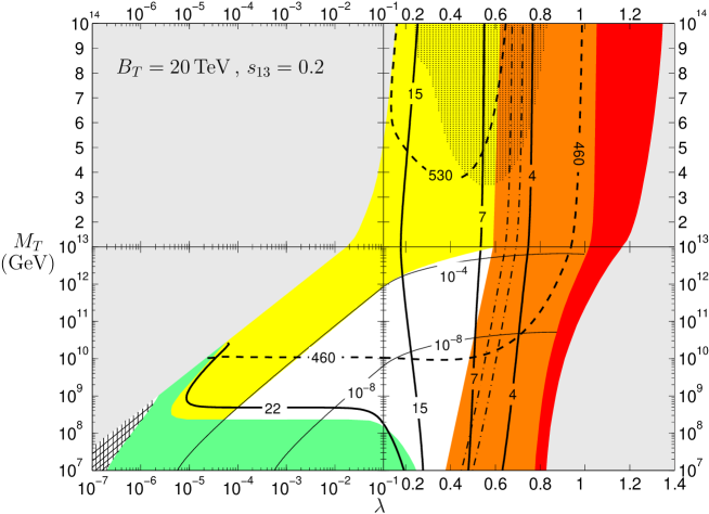
Figure 5: The $({\lambda},M_{T})$-parameter space configuration for $B_{T}=20$ TeV and $s_{13}=0~{}(s_{13}=0.2)$ in the upper (lower) panel. Perturbativity and EWSB exclude the light-grey and red regions (see legend in the upper panel), respectively. The orange region is excluded by the Higgs mass bound $m_{h}<$ 110 GeV for $m_{t}=170.2$ GeV, while the left-most (right-most) dash-dotted line delimit the same region for $m_{t}=172.5\,(174.8)$ GeV. Inside the yellow and green areas, ${\rm BR}(\mu\to e\gamma)$ is above the present experimental upper bound and the lightest slepton mass is below 100 GeV, respectively. In the dotted and hatched areas, the neutralino $\tilde{\chi}^{0}_{1}$ is the lightest MSSM sparticle and $\tilde{\ell}_{1}$ is tachyonic, respectively. The thick-solid (dashed) lines correspond to the isocontours of $\tan\beta$ ($\mu$ in GeV) for $m_{t}=172.5$ GeV. The thin solid lines refer to the FV parameter $\delta^{d}_{bs}$ [defined in Eq. (76)]. See text for more details.

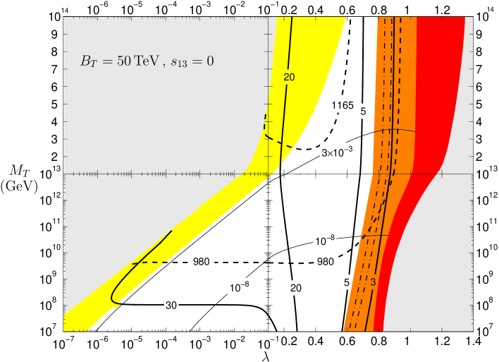
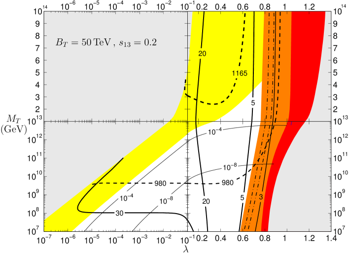
Figure 6: The same as in Fig. 5 for $B_{T}=50~{}{\rm TeV}$.

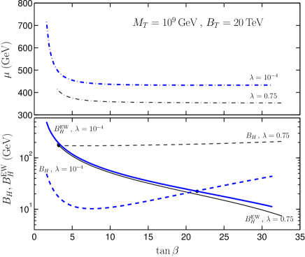
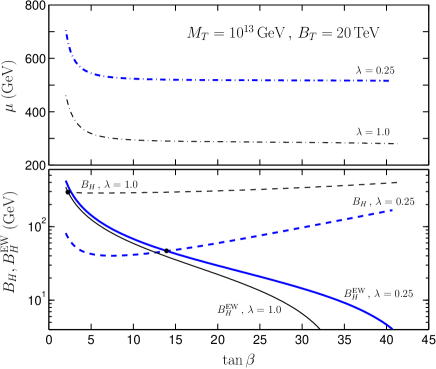
Figure 7: Left panel: Curves of $B_{H}$ (dashed lines) obtained at $\mu_{s}$ from the running of $B_{H}(M_{T})$, and of $B_{H}^{EW}$ (solid lines) determined by the minimization conditions (38), as a function of $\tan\beta$ for $B_{T}=20$ TeV, $M_{T}=10^{9}$ GeV and $\lambda=10^{-4},0.75$ (lower plot). In the upper plot, the corresponding values of the $\mu$ parameter are shown. Right panel: The same as in the left one but for $M_{T}=10^{13}$ GeV and $\lambda=0.25,1.0$.

The EWSB constraint excludes the red region (which covers the range with ${\lambda}\sim 1$ along the whole interval of $M_{T}$) limited on the left by the least achievable value of $\tan\beta\approx 2.5$. We have studied the sensitivity of our results to the top mass, considering the $1\sigma$ allowed range $m_{t}=(172.5\pm 2.3)$ GeV [50]. The most relevant effects of varying $m_{t}$ are the ones induced by the top-Yukawa term in the RG running of the soft mass $m^{2}_{H_{2}}$. However, this variation does not affect our results considerably and, therefore, we will mainly take the central value $m_{t}=172.5$ GeV.

The EWSB conditions select values of $\tan\beta$ (thick solid-contours) up to moderate ones, ($\tan\beta\lower 3.01385pt\hbox{$\;\stackrel{{\scriptstyle\textstyle<}}{{\sim}}\;$}25$). Notice that the largest values of $\tan\beta$ are achievable only for $M_{T}\lower 3.01385pt\hbox{$\;\stackrel{{\scriptstyle\textstyle<}}{{\sim}}\;$}10^{9}~{}{\rm GeV}$ and small values of ${\lambda}\lower 3.01385pt\hbox{$\;\stackrel{{\scriptstyle\textstyle<}}{{\sim}}\;$}0.2$. In fact, Eq. (38) shows that larger values of $\tan\beta$ (or smaller $\sin 2\beta$) require suppressed $B_{H}(\mu_{s})$, which can be obtained by shortening the running energy interval (and so, smaller $M_{T}$ are needed). We also display the iso-contours of the $\mu(\mu_{s})$ parameter (dashed-lines) as obtained by the EWSB conditions. One can realize that this parameter slightly increases with $M_{T}$ due to the enhancement of the RG factor which affects $m^{2}_{H_{2}}(\mu_{s})$ in the minimisation condition of Eq. (38). The whole allowed parameter space covers the range $\mu\sim(450-550)~{}{\rm GeV}$.

To better understand the behavior of the $\mu$ and $\tan\beta$ contours, it may be useful to consider Fig. 5 together with Fig. 7. Indeed, the latter displays the solutions of Eq. (38) for $\mu$ (upper plots) and $B_{H}$ (lower plots), when $M_{T}=10^{9}~{}(10^{13})~{}{\rm GeV}$ in the left (right) panel. We have chosen four distinct points in the $(\lambda,M_{T})$ parameter space and shown, for each case, the predicted parameter $B_{H}(\mu_{s})=B_{H}(M_{T})+\Delta B_{H}$, where $B_{H}(M_{T})$ is determined from Eqs. (16) and $\Delta B_{H}$ englobes the RG running between $M_{T}$ and $\mu_{s}$. The curves of $B_{H}(\mu_{s})$ have to be compared with those of $B_{H}$ as extracted from Eq. (38) (denoted by $B^{EW}_{H}$ in the plots). The crossing of these two curves (indicated by a black dot) signals the presence of a solution at the corresponding value of $\tan\beta$. For instance, the left-panel of Fig. 7 shows that for $B_{T}=20$ TeV, $M_{T}=10^{9}$ GeV and $\lambda=10^{-4}(0.75)$, EWSB occurs for $\tan\beta\approx 22(3)$ with $\mu\approx 450(400)$ GeV. A similar example is illustrated in the right-panel of Fig. 7 for $B_{T}=20$ TeV, $M_{T}=10^{13}$ GeV and $\lambda=0.25$ and 1.

Consider now the constraint imposed by the lower bound on $m_{h}$. The orange region in Fig 5 shows the portion of the parameter space forbidden by the condition $m_{h}>110$ GeV, taking the lower limit of the $1\sigma$ range for the top-mass ($m_{t}=170.2$ GeV). The dependence on $m_{t}$ comes from the low-energy radiative corrections $\propto\frac{m^{4}_{t}}{m^{2}_{W}}{\rm ln}(\mu^{2}_{s}/m^{2}_{t})$. As $m_{t}$ increases, the region shrinks, being delimited by the left-most (right-most) dashed-line when $m_{t}=172.5\,(174.8)$ GeV. It is also clear that, for each value of $M_{T}$, the upper bound on $\lambda$ is set by the Higgs mass constraint e.g., $\lambda<0.45-0.55$ when $M_{T}=10^{9}$ GeV. Since the dependence of the Higgs mass on $\tan\beta$ mostly comes from the tree-level contribution $|\cos 2\beta|M_{Z}$, the iso-contours of $m_{h}$ closely follow those of $\tan\beta$, setting in this way the least allowed value of $\tan\beta\approx 7$.

In our framework, the lightest MSSM supersymmetric particle is tipically the lightest slepton $\tilde{\ell}_{1}$, except inside the dotted region where $m_{\tilde{\chi}^{0}_{1}}<m_{\tilde{\ell}_{1}}$ (which is almost entirely excluded by the Higgs and $\mu\rightarrow e\gamma$ constraints). The mass of $\tilde{\ell}_{1}$ turns out to be below the LEP2 lower bound of about $100$ GeV in the region of the parameter space filled in green, where the large values of $\tan\beta\lower 3.01385pt\hbox{$\;\stackrel{{\scriptstyle\textstyle>}}{{\sim}}\;$}22$ reduce $m_{\tilde{\ell}_{1}}$ through the left-right mixing at the electroweak-symmetry breaking (see also Section 7.1). In the hatched region (lower-left corner), where $\tan\beta\approx 30$, the lightest slepton is tachyonic.

All the constraints discussed so far, being related to ‘unflavoured’ observables, are not sensitive to the angle $\theta_{13}$, as it is shown by the comparison between the upper ($\sin\theta_{13}=0$) and lower ($\sin\theta_{13}=0.2$) panels of Fig. 5. On the contrary, the size of LFV strongly depends on it [see Eq. (5)] and hence, the region excluded by the bound on ${\rm BR}(\mu\to e\gamma)$ changes when different values of $\theta_{13}$ are considered. For $M_{T}\lower 3.01385pt\hbox{$\;\stackrel{{\scriptstyle\textstyle>}}{{\sim}}\;$}2\times 10^{8}~{}{\rm GeV}$, the $\mu\rightarrow e\gamma$ constraint provides the most restrictive lower bound on ${\lambda}$. This stems from the fact that the size the LFV entry $({\bf m}^{2}_{\tilde{L}})_{\mu e}$ scales as $(M_{T}/{\lambda})^{2}$ [Eq. (5)]. Consequently, the allowed ${\lambda}$ range is wider for lower values of $M_{T}$, closing up for $M_{T}\sim 4\times 10^{13}~{}{\rm GeV}$. By switching on $s_{13}$ (lower panel), the size of $\mu e$ LFV is enhanced as

$$\frac{({\bf m}^{2}_{\tilde{L}})_{\mu e}|^{s_{13}=0.2}}{({\bf m}^{2}_{\tilde{L}})_{\mu e}|^{s_{13}=0}}\approx 1+\left(\frac{\Delta m^{2}_{A}}{\Delta m^{2}_{S}}\right)^{2}\frac{s_{13}}{s_{12}c_{12}}\sim 12$$ (40)

and, correspondingly, the $\mu\to e\gamma$ limit implies that the lower bound on ${\lambda}$ increases by a factor of $\sim(140)^{1/4}\approx 3.5$ and so, the allowed parameter space shrinks. Taking into account all the constraints considered above, one concludes that values of $M_{T}\lower 3.01385pt\hbox{$\;\stackrel{{\scriptstyle\textstyle>}}{{\sim}}\;$}2\times 10^{13}{\rm GeV}$ are excluded for $B_{T}=20$ TeV, independently of the value of $\lambda$.

An equivalent analysis is presented in Fig. 6 for $B_{T}=50$ TeV. The comparison with the previous case indicates that the regions excluded by the perturbativity and EWSB requirements are not significantly affected. On the other hand, the constraint on the Higgs mass implies a slightly different upper bound on ${\lambda}$ (${\lambda}\lower 3.01385pt\hbox{$\;\stackrel{{\scriptstyle\textstyle<}}{{\sim}}\;$}0.6$) and a decrease of the minimum allowed value of $\tan\beta$ ($\tan\beta\lower 3.01385pt\hbox{$\;\stackrel{{\scriptstyle\textstyle>}}{{\sim}}\;$}4$). Indeed, the sparticle spectrum is now heavier and thus, the radiative corrections $\sim{\rm ln}(\frac{\mu_{s}^{2}}{m_{t}^{2}})$ to $m_{h}$ are larger. For this reason, smaller values of $\tan\beta$ are tolerated in the tree-level contribution $\sim M_{Z}|\cos 2\beta|$. Contrarily to the previous case, ${\tilde{\ell}}_{1}$ is never tachyonic and its mass lies above the LEP bound. Consequently, for $M_{T}=10^{7}-10^{8}\,{\rm GeV}$ the allowed ${\lambda}$-range is much more extended with respect to the case with $B_{T}=20~{}{\rm TeV}$. Moreover, larger values of $\tan\beta$ are now possible ($\tan\beta\lower 3.01385pt\hbox{$\;\stackrel{{\scriptstyle\textstyle<}}{{\sim}}\;$}40$). The heavier spectrum also makes the $\mu\to e\gamma$ constraint weaker, reducing the excluded yellow region. In conclusion, the allowed parameter space enlarges when $B_{T}$ increases. Also for this case, the effect of non-zero $\theta_{13}$ (lower panel) produces similar results as for smaller $B_{T}$, by raising the lower bound of ${\lambda}$.

Before concluding this section, a comment is in order about the influence of the type of neutrino spectrum on the allowed parameter space. In the IH case, the perturbativity constraint on the Yukawa couplings ${\bf Y}_{T,S,Z}$ would just imply a slightly larger minimum of ${\lambda}$, for each $M_{T}$. All other constraints would instead be unaffected. For a QD spectrum, the effect from the perturbativity requirement would be much stronger (depending on the magnitude of the overall neutrino mass $m_{1}$) since, as already mentioned, all the ${\bf Y}_{T,S,Z}$ entries increase when compared to the NH or IH cases. Therefore, the light-grey region would mostly cover the yellow area excluded by the ${\rm BR}(\mu\to e\gamma)$ bound. In conclusion, either for the IH or QD spectrum, the resulting allowed parameter space would not be much different from the NH case displayed in Figs. 5 and 6.

7 Phenomenological predictions

After describing the main phenomenological constraints imposed on the $(\lambda,M_{T})$ parameters space, we will now go through the specific features of the sparticle and Higgs spectra (Section 7.1) of our scenario, and to the implications for several low-energy LFV processes (Section 7.2).

7.1 Sparticle and Higgs spectroscopy

The spectrum of the superpartners is determined by the finite radiative contributions to the SSB parameters at $M_{T}$ (see Section 4), acting as boundary conditions, and by the subsequent MSSM RG running from $M_{T}$ to $\mu_{s}$. The physical scalar masses are obtained by taking into account the latter effect at one-loop level [51] and the low-energy $D$ and $F$-term contributions. To get some intuition on the main features of the physical spectrum, we present some qualitative arguments in addition to the complete numerical results.

In the present framework, the boundary conditions for the gaugino and sfermion masses are not universal at $M_{T}$, even when $M_{T}$ is not far from $M_{G}$. This is due to the different gauge quantum numbers of the MSSM field representations [see Eq. (4)]. At lowest order, the gaugino masses $\overline{M}_{a}$ at the messenger scale are in proportion to the gauge coupling squared, $\overline{M}_{1}:\overline{M}_{2}:\overline{M}_{3}=\overline{\alpha}_{1}:\overline{\alpha}_{2}:\overline{\alpha}_{3}$ ($\alpha_{a}=g^{2}_{a}/4\pi$). This relation is maintained at low-energy, like in unified SUGRA scenarios. The low-energy gaugino masses are given by:

$$M_{a}(\mu_{s})=\frac{B_{T}}{16\pi^{2}}\,N\,g_{a}^{2}(\mu_{s}),~{}~{}~{}~{}~{}a=1,2,3\,,$$ (41)

which leads to: $M_{2}\approx 1.86\,M_{1}\approx 0.35\,M_{3}$ (taking $\mu_{s}\sim 700\,{\rm GeV})$. The most interesting aspect comes from the fact that the scalar and gaugino masses are mutually related at the messenger scale. For the sake of our discussion, let us disregard for the moment the contributions proportional to the Yukawa couplings in the expressions of the scalar masses in Eqs. (4), as well as the Yukawa effects in the (1-loop) renormalization. In such a case, the low-energy sfermion masses have the form:

$${\bf m}^{2}_{{\tilde{f}}}(\mu_{s}) = \frac{2k_{a}C^{f}_{a}}{N}~{}\overline{M}^{2}_{a}+\Delta R_{a}\;\;\;,\;\;\;$$

$$\Delta R_{a} = \overline{M}^{2}_{a}\frac{2k_{a}C^{f}_{a}(1-x_{a})}{b_{a}}\;\;\;,\;\;\;x_{a}=\frac{g^{4}_{a}(\mu_{s})}{\bar{g}^{4}_{a}},$$ (42)

where $b_{1}=33/5,b_{2}=1,b_{3}=-3$. The first term in ${\bf m}^{2}_{{\tilde{f}}}(\mu_{s})$ corresponds to the high-energy boundary contribution while the second one, $\Delta R_{a}$, accounts for the RG effects induced by the gaugino masses. The squark masses $m_{\tilde{Q}}$ receive the main RG correction from the gluino mass term, which amounts to a positive shift on $m_{\tilde{Q}}^{2}$. The term $\Delta R_{3}$ is larger than the boundary condition value (since $|1-x_{3}|>|b_{a}|/N=3/7$), by a factor of approximately $8~{}(2)$ for $M_{T}=10^{14}~{}(10^{7})~{}{\rm GeV}$. Notice that, in the minimal GMSB model ($N=1$), the dominance of $\Delta R_{3}$ holds only for a messenger scale above $\sim 10^{12}~{}{\rm GeV}$  [52]. Therefore, we expect the low-energy ratio $m_{{\tilde{Q}}}/M_{3}$ to be given as

$$\frac{m_{\tilde{Q}}}{M_{3}}\approx\left\{\frac{2C^{q}_{3}}{b_{3}}\frac{1-x_{3}}{x_{3}}\,\left[1+\frac{b_{3}}{N(1-x_{3})}\right]\right\}^{1/2}\,,$$ (43)

which lies within $0.9-0.8$ for $M_{T}\sim 10^{14}-10^{7}~{}{\rm GeV}$. Hence, the gluino is the heaviest of the coloured sparticles.

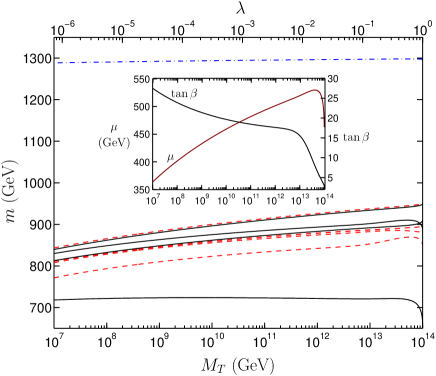
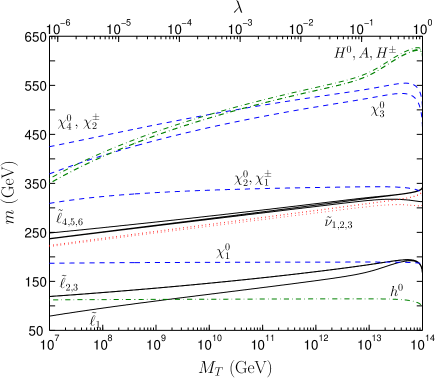
Figure 8: The sparticle and Higgs spectrum for $B_{T}=20~{}{\rm TeV}$ as a function of $M_{T}$ and correspondingly taking ${\lambda}$ (as indicated in the upper horizonal axis) along the isocontour ${\rm BR}({\mu\rightarrow e\gamma})=1.2\times 10^{-11}$. Left panel: physical squark masses, $m_{\tilde{u}}$ (black solid lines), $m_{\tilde{d}}$ (red dashed) and the pole gluino mass $m_{\tilde{g}}$ (blue dash-dotted). Right panel: charged slepton masses $m_{\tilde{\ell}}$ (solid black lines), sneutrino masses $m_{\tilde{\nu}}$ (dotted blue), neutralino and chargino masses $m_{\tilde{\chi}^{0}}$ and $m_{\tilde{\chi}^{\pm}}$ (dashed blue). The dash-dotted green lines correspond to the Higgs boson masses $m_{h},m_{H},m_{A}$ and $m_{H^{\pm}}$. In the small inner plot (on the left panel) we show the behavior of $\tan\beta$ (red line) and $\mu$ as obtained by the EWSB conditions.

In Fig. 8 we display the sparticle and Higgs spectra for $B_{T}=20~{}{\rm TeV}$. The values of $\lambda$ (shown in the upper horizontal axis) and $M_{T}$, are the ones along the border which delimits on the right the $\mu\to e\gamma$ excluded region (see upper panel of Fig. 5). The gluino pole mass includes the low-energy finite corrections (see e.g. [53]), which ammount to $20-30\,\%$ of the tree-level value $M_{3}$. As anticipated the gluino is the heaviest superparticle. The first and second generation squarks $\tilde{d}$ (dashed curves) and $\tilde{u}$ (solid) (mainly composed by left-handed squarks) are the heaviest. Instead, the lightest squark $\tilde{t}_{1}$ is mainly a right-handed $\tilde{t}^{c}$ whose mass is pushed down by a negative shift, driven mainly by the top Yukawa-induced renormalization. This effect, together with the left-right squark mixing, is enhanced for $M_{T}\lower 3.01385pt\hbox{$\;\stackrel{{\scriptstyle\textstyle>}}{{\sim}}\;$}10^{13}~{}{\rm GeV}$ where $\tan\beta$ becomes smaller (see the inner panel where we have drawn the behavior of $\tan\beta$ and $\mu$ versus $M_{T}$). This analysis has shown that for $B_{T}=20~{}{\rm TeV}$ in the allowed $({\lambda},M_{T})$ portion, where the $\mu\to e\gamma$ is close to the present bound, the squark spectrum lies in the range $800-950~{}{\rm GeV}$. This mass range will be soon explored by the Large Hadron Collider (LHC) [54] with a luminosity $\mathcal{L}=100$ pb^-1 and a center-of-mass energy $\sqrt{s}=14$ TeV.

The left-handed slepton masses can instead be compared with the $SU(2)_{W}$ gaugino mass $M_{2}$. In this case the renormalization factor in Eq. (7.1) is comparable to the boundary contribution. At low-energy, the ratio $m_{{\tilde{L}}}/M_{2}$ lies in the range $1-0.5$ for $M_{T}=10^{14}-10^{7}~{}{\rm GeV}$. In the right panel of Fig. 8 we show the physical spectrum of the electroweak states. The heaviest charged sleptons $\tilde{\ell}_{4,5,6}$ (which are mainly left-handed sleptons) have masses around $250-320~{}{\rm GeV}$ in the allowed range $M_{T}\sim 10^{8}-10^{13}~{}{\rm GeV}$. The sneutrino masses are splitted from the latter states mainly by the $SU(2)_{W}$ $D-$term, $m^{2}_{\tilde{\ell}}-m^{2}_{\tilde{\nu}}=m^{2}_{W}|\cos 2\beta|$.

The right-handed slepton masses receive contributions only from the $U(1)_{Y}$ gauge interactions and, therefore, are smaller than the other sfermion masses. In the range $M_{T}=10^{14}-10^{7}~{}{\rm GeV}$, the high energy contribution is larger than the renormalization term $\Delta R_{1}$ by a factor of $\sim 1-3$. The low-energy ratio $m_{{\tilde{e^{c}}}}/M_{1}$ is approximately in the range $1-0.7$ for $M_{T}=10^{14}-10^{7}~{}{\rm GeV}$. To these estimates one has to add the negative shift from the $Y_{\tau}$-induced renormalization and the effect from the left-right slepton mixing at the electroweak-symmetry breaking. Both these contributions are important for large $\tan\beta$ and lower the physical $\tilde{\tau}_{1}$ mass below $m_{\tilde{\tau}^{c}}$. In Fig. 8 (right panel) we can see that for $M_{T}\lower 3.01385pt\hbox{$\;\stackrel{{\scriptstyle\textstyle<}}{{\sim}}\;$}10^{8}~{}{\rm GeV}$ the $\tilde{\tau}_{1}$ mass is pushed below $100~{}{\rm GeV}$ and, in the range $M_{T}\sim 10^{8}-10^{13}~{}{\rm GeV}$, $\tilde{\tau}_{1}$ is indeed the lightest MSSM sparticle. For larger values of $M_{T}$, corresponding to small $\tan\beta$, the neutralino $\tilde{\chi}^{0}_{1}$ becomes the lightest MSSM sparticle. Hence, either $\tilde{\tau}_{1}$ or $\tilde{\chi}^{0}_{1}$ would decay into the gravitino, which is in fact the lightest SUSY particle in our framework. In conclusion, the slepton masses lie in the range $\sim 100-320$ GeV (for $B_{T}=20$ TeV) and, therefore, are within the discovery potential of the LHC.

Concerning the physical charginos and neutralinos, the inner plot (right panel) shows that the parameter $\mu$ comes out to be larger than $M_{Z}$ and $\mu^{2}-M^{2}_{1,2}>M^{2}_{Z}$ hold for most of the parameter space. These hierarchies imply that the lightest neutralino $\tilde{\chi}^{0}_{1}$ is mainly a $B$-ino and has mass $m_{\tilde{\chi}^{0}_{1}}\approx M_{1}$ , while $\tilde{\chi}^{0}_{2}$ and the lightest chargino $\tilde{\chi}^{\pm}_{1}$ are almost degenerate and are mainly $W$-inos with mass $\approx M_{2}$ [30]. Therefore, both these masses do not exhibit a significant dependence on $M_{T}$, as seen in Fig. 8 (right panel). The heaviest chargino $\tilde{\chi}^{\pm}_{2}$ and neutralinos $\tilde{\chi}^{0}_{3,4}$ are mostly higgsinos with mass set by the $\mu$ parameter, increasing therefore with $M_{T}$.

Notice that, increasing the value of $B_{T}$, all the sparticles become linearly heavier since they scale as $B_{T}$.

Finally, also the Higgs boson masses can be predicted in our scenario. As already mentioned in Section 6.1, the mass of the lightest CP-even Higgs boson ($m_{h}$ ) has been computed by including the low-energy radiative corrections. In the allowed parameter space of Fig.5, $m_{h}$ turns out to be in the range $110-120~{}{\rm GeV}$, thus being testable in the near future at the LHC (mainly through the Higgs decay into 2 photons [55]). The heaviest CP-even ($H$), CP-odd ($A$) and charged Higgs bosons are much heavier. At tree-level, $m_{A}=\mu B_{H}/\sin 2\beta$ and for $m_{A}\gg M_{Z}$ all these states are almost degenerate, $m_{H}\sim m_{H^{\pm}}\sim m_{A}$. For $B_{T}=20~{}{\rm TeV}$, Fig. 8 shows that $m_{A},m_{H},m_{H^{\pm}}\approx 400-470~{}{\rm GeV}$. For larger values of $B_{T}$ the masses of such non-standard Higgs bosons increase, while $m_{h}$ increases by a few GeV due to the logarithmic sensitivity to $B_{T}$. The Higgs sector is therefore characterized by a decoupling regime with a light SM-like Higgs boson ($h$) and the three heavy states ($H,A,H^{\pm}$).

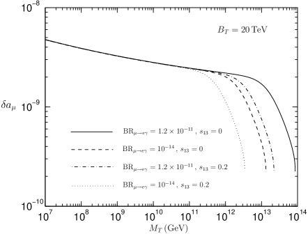
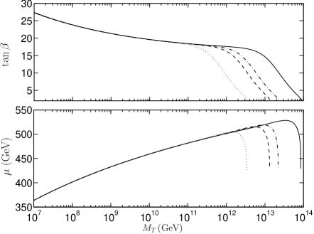
Figure 9: Left panel: SUSY muon anomalous magnetic moment contribution $\delta a_{\mu}$ as a function of $M_{T}$ (taken with its corresponding ${\lambda}$ along the lines of constant ${\rm BR}({\mu\rightarrow e\gamma})=1.2\times 10^{-11},10^{-14}$) for $s_{13}=0,0.2$ and $B_{T}=20$ TeV. Right panel: curves of $\mu$ (lower plot) and $\tan\beta$ (upper plot), for the same inputs considered in the left-panel.

We conclude this section with a comment on the SUSY contribution to the muon anomalous magnetic moment $\delta a_{\mu}$. In Fig. 9 we show the $\delta a_{\mu}$ behavior as a function of $M_{T}$ in correspondence with different values of ${\rm BR}({\mu\rightarrow e\gamma})$ and for $B_{T}=20$ TeV. It is well known that $\delta a_{\mu}$ is induced by the dipole operator whose dominant contributions go as $\sim\frac{g^{2}m_{\mu}^{2}\mu\tan\beta}{16\pi^{2}m^{3}_{soft}}$. Since the sparticle spectrum does not change significantly with $M_{T}$ (Fig. 8), $\delta a_{\mu}$ directly reflects the demeanor of $\tan\beta$ (cf. left and right panels). The sign of $\delta a_{\mu}$ is the same as the one of $\mu$ and, in the allowed range $M_{T}\lower 3.01385pt\hbox{$\;\stackrel{{\scriptstyle\textstyle>}}{{\sim}}\;$}2\times 10^{8}$ GeV, $\delta a_{\mu}\lower 3.01385pt\hbox{$\;\stackrel{{\scriptstyle\textstyle<}}{{\sim}}\;$}4\times 10^{-9}$ respects the constraint (39). As $\delta a_{\mu}$ scales as $1/B_{T}^{2}$, it decreases for larger $B_{T}$.

7.2 LFV: Model Independent Predictions

We have already described the structure and parameter dependence of the flavour violating SSB mass parameters in Section 5. Here, we intend to further investigate the phenomenological implications by considering several LFV processes (besides $\mu\to e\gamma$) such as, $\mu\to eee,\tau\to\mu\gamma,\tau\to e\gamma,\tau\to\mu\mu\mu,\tau\to eee,\tau\to\mu ee\,\tau\to e\mu\mu$ and $\mu\to e$ conversion in ${}^{22}_{48}{\rm Ti}$. The present experimental upper bounds and future sensitivities for the BRs of these decays are collected in Table 1.

Let us briefly recall some points related to the computation of such processes. The radiative decays $\ell_{j}\to\ell_{i}+\gamma$ are induced by the effective dipole operator:

$$em_{j}(iD^{L}_{ji}\bar{\ell}_{i}\bar{\sigma}^{\rho\sigma}\bar{\ell}^{c}_{j}+iD^{R}_{ji}{\ell}^{c}_{i}{\sigma}^{\rho\sigma}\ell_{j}+{\rm h.c.})F_{\rho\sigma}\,,$$ (44)

where $e$ and $F_{\rho\sigma}$ are the electric charge and the electromagnetic field strength, respectively. The corresponding branching ratios are:

$${\rm BR}(\ell_{j}\to\ell_{i}+\gamma)=\frac{48\pi^{3}\alpha}{G^{2}_{F}}\left[|D^{L}_{ji}|^{2}+|D^{R}_{ji}|^{2}\right]~{}{\rm BR}(\ell_{j}\to\ell_{i}\nu_{j}\bar{\nu}_{i})\,,$$ (45)

where $\alpha=e^{2}/(4\pi)$, $G_{F}$ is the Fermi constant, ${\rm BR}(\mu\to e\nu_{\mu}\bar{\nu}_{e})\approx 1,\,{\rm BR}(\tau\to\mu\nu_{\tau}\bar{\nu}_{\mu})\approx 17\%$ and ${\rm BR}(\tau\to e\nu_{\tau}\bar{\nu}_{e})\approx 18\%$. Since LFV resides in the parameters ${\bf m}^{2}_{\tilde{L}}$ and ${\bf A}_{e}$, the coefficient $D^{L}$ is the dominant one. In the mass-insertion approximation its parametric dependence is:

$$D^{L}_{ji}\sim\frac{g^{2}}{16\pi^{2}}\frac{1}{m^{2}_{soft}}\left[\frac{({\bf m}^{2}_{\tilde{L}})_{ji}}{m^{2}_{\rm soft}}~{}~{}{\rm or}~{}~{}\frac{({\bf m}^{2}_{\tilde{L}})_{ji}}{m^{2}_{\rm soft}}\tan\beta~{}~{}{\rm or}~{}~{}\frac{({\bf A}_{e})_{ji}}{({\bf Y}_{e})_{jj}m_{\rm soft}}\right],$$ (46)

where the coupling $g$ can be either $g_{2}$ or $g^{\prime}=\sqrt{3/5}g_{1}$. In the MSSM framework, the dipole coefficient $D^{L}$ receives contributions from three different diagram topologies which, under certain features of the sparticle spectrum, could cancel against each other. In the latter case, these decays would be strongly suppressed even if the sparticle spectrum were not too heavy [56]. This can be realized if, for instance, the A-terms ${\bf A}_{e}$ are large, or the gaugino mass parameters $M_{1}$ and $M_{2}$ have opposite sign. In our scenario such peculiar situations do not occur, so the suppression of the dipole operators can only arise from large mass parameters (i.e. by increasing $B_{T}$) or from cancelations inherent to the ${\bf m}^{2}_{\tilde{L}}$ off-diagonal entries, as discussed in Section 5.

The strict predictions regarding the ratios (5) and (5) can be translated into predictions for the ratios of the BRs [9] once Eqs. (45) and (46) are taken into account:

$$\frac{{\rm BR}(\tau\to\mu\gamma)}{{\rm BR}(\mu\to e\gamma)} \approx \left[\frac{({\bf m}^{2}_{{\tilde{L}}})_{\tau\mu}}{({\bf m}^{2}_{{\tilde{L}}})_{\mu e}}\right]^{2}\frac{{\rm BR}(\tau\to\mu\nu_{\tau}\bar{\nu}_{\mu})}{{\rm BR}(\mu\to e\nu_{\mu}\bar{\nu}_{e})}\approx\left\{\begin{array}[]{l}300\quad\quad\quad\quad[s_{13}=0]\\ \\ 2\,(3)\!\!\quad\quad\quad\quad[s_{13}=0.2]\end{array}\right.\,$$ (50)

$$\frac{{\rm BR}(\tau\to e\gamma)}{{\rm BR}(\mu\to e\gamma)} \approx \left[\frac{({\bf m}^{2}_{{\tilde{L}}})_{\tau e}}{({\bf m}^{2}_{{\tilde{L}}})_{\mu e}}\right]^{2}\frac{{\rm BR}(\tau\to e\nu_{\tau}\bar{\nu}_{e})}{{\rm BR}(\mu\to e\nu_{\mu}\bar{\nu}_{e})}\approx\left\{\begin{array}[]{l}0.2\quad\quad\quad\quad\,\,\,\,[s_{13}=0]\\ \\ 0.1~{}(0.3)\,\,\quad\quad[s_{13}=0.2]\end{array}\right.\,,$$ (54)

where the results on the r.h.s hold for all the three types of neutrino mass spectrum and the numbers in parenthesis apply for IH case, whenever this is different from the others.

Regarding the 3-body decays $\ell_{j}\to\ell_{i}\ell_{k}\ell_{k}$ and $\mu\to e$ conversion in Ti, these receive contributions from $\gamma$- (dipole $D^{L,R}$ and monopole $C^{L,R}$ operators), $Z$- (monopole $A^{L,R}$ operator) and Higgs- (monopole $\Delta^{L,R}$ operator) exchange diagrams, as well as from box ($B^{LL,RR},\,B^{LR,RL}$) diagrams. The branching ratios are given by:

$${\rm BR}(\ell_{j}^{-}\to\ell_{i}^{-}\ell_{k}^{+}\ell_{k}^{-}) = \frac{1}{8G^{2}_{F}}\left\{a_{k}|F^{LL}_{ji}|^{2}+|F^{LR}_{ji}|^{2}+|F^{RL}_{ji}|^{2}+a_{k}|F^{RR}_{ji}|^{2}+\right.$$ (56)

$$\left.+4e^{2}{\rm Re}\left[D^{L}_{ji}(a_{k}\bar{F}^{LL}_{ji}+\bar{F}^{LR}_{ji})+D^{R}_{ji}(\bar{F}^{RL}_{ji}+a_{k}\bar{F}^{RR}_{ji})\right]\right.$$

$$\left.+8e^{4}(|D^{L}_{ji}|^{2}+|D^{R}_{ji}|^{2})\left({\rm log}\frac{m^{2}_{j}}{m^{2}_{k}}-b_{k}\right)\right\}{\rm BR}(\ell_{j}^{-}\to\ell_{i}^{-}\bar{\nu}_{i}\nu_{j})\,,$$

where $a_{k}=1(2),~{}b_{k}=3(11/4)$ for $k\neq i\,(k=i)$, and the coefficients $F^{NP}\,(N,P=L,R)$ are combinations of $A^{N},B^{NP},C^{N}$ and $\Delta^{N}$ (see e.g. [56]). We have found some discrepancies between our analytical computations concerning the coefficients $A^{L,R}$ with those published by some authors [11]. In Appendix 2 we have reported and discussed our results for $A^{L,R}$. Moreover, in Appendix 3 we present the results for the box coefficients $B^{MN}$ relevant for the decays $\tau\to\mu ee$ and $\tau\to e\mu\mu$, calculated to all order in the electroweak-breaking effects. For the sake of brevity, we refer to the existing literature (e.g. [11] and [56]) for the explicit formulas of all the other coefficients, including the one relevant for the CR($\mu\to e\,$; Ti). Like for the dipole $D^{L}$, the presence of LFV in the left-handed sector implies that only the coefficients $A^{L},B^{LL},B^{LR},C^{L},\Delta^{L}$ are important. We just recall their parametric dependence:

$$A^{L}_{ji}\,,\,\frac{B^{LL(LR)}_{ji}}{g^{2}}\,,\,C^{L}_{ji}\,\sim\,\frac{g^{2}}{16\pi^{2}}\frac{({\bf m}^{2}_{\tilde{L}})_{ji}}{m^{4}_{soft}}\quad\quad,\quad\quad\Delta^{L}_{ji}\sim\frac{g^{2}}{16\pi^{2}}\frac{({\bf m}^{2}_{\tilde{L}})_{ji}}{m^{2}_{soft}}.$$ (57)

From what has been commented above about suppressing $D^{L}$ in our scenario, and by comparing Eq. (46) with (57), one can realize that, whenever the coefficients $D^{L}$ get suppressed, $A^{L},B^{LL,LR}$ and $C^{L}$ undergo the same fate. Regarding $\Delta^{L}$, one has that $\Delta^{L}_{ji}\to 0$ only if $({\bf m}^{2}_{\tilde{L}})_{ji}\to 0$ since these coefficients are insensitive to an overall mass scale increasing. Consequently, the $D^{L}$ contributions to the 3-body BRs [CR$(\mu\to e)$] are dominant with respect to those from the remaining operators, due to the $\tan\beta$ and phase-space logarithmic-factor [$\tan\beta$] enhancement.

Although the Higgs-exchange diagram contribution also benefits from a $\tan\beta$ enhancement, its numerical relevance requires the Higgs bosons $A$ and $H$ to be significantly lighter than the sleptons, charginos and neutralinos [57, 58, 56, 59]. As already discussed in Section 7.1, in our scenario this does not occur, thus the Higgs-mediated contributions come out to be subleading.

In the aforementioned dipole-dominance situation, the LFV processes under consideration can be directly compared with the radiative decays:

$$\frac{{\rm BR}(\mu\to eee)}{{\rm BR}(\mu\to e\gamma)} \approx \frac{\alpha}{3\pi}\left({\rm ln}\frac{m^{2}_{\mu}}{m^{2}_{e}}-\frac{11}{4}\right)\approx 6\times 10^{-3},$$

$$\frac{{\rm BR}(\tau\to eee)}{{\rm BR}(\tau\to e\gamma)} \approx \frac{\alpha}{3\pi}\left({\rm ln}\frac{m^{2}_{\tau}}{m^{2}_{e}}-\frac{11}{4}\right)\approx 10^{-2},$$

$$\frac{{\rm BR}(\tau\to e\mu\mu)}{{\rm BR}(\tau\to e\gamma)} \approx \frac{\alpha}{3\pi}\left({\rm ln}\frac{m^{2}_{\tau}}{m^{2}_{\mu}}-3\right)\approx 2\times 10^{-3},$$

$$\frac{{\rm BR}(\tau\to\mu\mu\mu)}{{\rm BR}(\tau\to\mu\gamma)} \approx \frac{\alpha}{3\pi}\left({\rm ln}\frac{m^{2}_{\tau}}{m^{2}_{\mu}}-\frac{11}{4}\right)\approx 2.2\times 10^{-3},$$

$$\frac{{\rm BR}(\tau\to\mu ee)}{{\rm BR}(\tau\to\mu\gamma)} \approx \frac{\alpha}{3\pi}\left({\rm ln}\frac{m^{2}_{\tau}}{m^{2}_{e}}-3\right)\approx 10^{-2},$$

$$\frac{{\rm CR}(\mu\to e\,;\,{\rm Ti})}{{\rm BR}(\mu\to e\gamma)} \approx 16\,\alpha^{4}Z_{\rm eff}^{4}Z|F(q)|^{2}\frac{\Gamma_{\mu}}{\Gamma_{\rm capt}^{\rm Ti}}\approx 5\times 10^{-3}\,,$$ (58)

where $Z=22$, $Z_{\rm eff}=17.6$, $|F(q)|^{2}\approx 0.54$, $\Gamma_{\rm capt}^{\rm Ti}\approx 2.6\times 10^{6}\,{\rm s}^{-1}$ is the muon capture width in Ti [11] and $\Gamma_{\mu}\approx 4.5\times 10^{5}\,{\rm s}^{-1}$ is the total muon decay width. In addition to these correlations, we also find that the 3-body decays can be related to each other by using the ratios (5) as follows:

$$\frac{{\rm BR}(\tau\to\mu\mu\mu)}{{\rm BR}(\mu\to eee)} \approx \left[\frac{({\bf m}^{2}_{{\tilde{L}}})_{\tau\mu}}{({\bf m}^{2}_{{\tilde{L}}})_{\mu e}}\right]^{2}\left(\frac{{\rm ln}\frac{m^{2}_{\tau}}{m^{2}_{\mu}}-\frac{11}{4}}{{\rm ln}\frac{m^{2}_{\mu}}{m^{2}_{e}}-\frac{11}{4}}\right)\frac{{\rm BR}(\tau\to\mu\nu_{\tau}\bar{\nu}_{\mu})}{{\rm BR}(\mu\to e\nu_{\mu}\bar{\nu}_{e})}\approx\left\{\begin{array}[]{ll}100&[s_{13}=0]\\ \\ 0.6~{}(0.9)&[s_{13}=0.2]\end{array}\right.$$ (62)

$$\frac{{\rm BR}(\tau\to\mu ee)}{{\rm BR}(\mu\to eee)} \approx \left[\frac{({\bf m}^{2}_{{\tilde{L}}})_{\tau\mu}}{({\bf m}^{2}_{{\tilde{L}}})_{\mu e}}\right]^{2}\left(\frac{{\rm ln}\frac{m^{2}_{\tau}}{m^{2}_{e}}-3}{{\rm ln}\frac{m^{2}_{\mu}}{m^{2}_{e}}-\frac{11}{4}}\right)\frac{{\rm BR}(\tau\to\mu\nu_{\tau}\bar{\nu}_{\mu})}{{\rm BR}(\mu\to e\nu_{\mu}\bar{\nu}_{e})}\approx\left\{\begin{array}[]{ll}550&\quad\,\,\,\,[s_{13}=0]\\ \\ 3~{}(4)&\quad\,\,\,\,[s_{13}=0.2]\end{array}\right.$$ (66)

$$\frac{{\rm BR}(\tau\to eee)}{{\rm BR}(\mu\to eee)} \approx \left[\frac{({\bf m}^{2}_{{\tilde{L}}})_{\tau e}}{({\bf m}^{2}_{{\tilde{L}}})_{\mu e}}\right]^{2}\left(\frac{{\rm ln}\frac{m^{2}_{\tau}}{m^{2}_{e}}-\frac{11}{4}}{{\rm ln}\frac{m^{2}_{\mu}}{m^{2}_{e}}-\frac{11}{4}}\right)\frac{{\rm BR}(\tau\to e\nu_{\tau}\bar{\nu}_{e})}{{\rm BR}(\mu\to e\nu_{\mu}\bar{\nu}_{e})}\sim\left\{\begin{array}[]{ll}0.3&\,\,[s_{13}=0]\\ \\ 0.2~{}(0.4)&\,\,[s_{13}=0.2]\end{array}\right.$$ (70)

$$\frac{{\rm BR}(\tau\to e\mu\mu)}{{\rm BR}(\mu\to eee)} \approx \left[\frac{({\bf m}^{2}_{{\tilde{L}}})_{\tau e}}{({\bf m}^{2}_{{\tilde{L}}})_{\mu e}}\right]^{2}\left(\frac{{\rm ln}\frac{m^{2}_{\tau}}{m^{2}_{\mu}}-3}{{\rm ln}\frac{m^{2}_{\mu}}{m^{2}_{e}}-\frac{11}{4}}\right)\frac{{\rm BR}(\tau\to e\nu_{\tau}\bar{\nu}_{e})}{{\rm BR}(\mu\to e\nu_{\mu}\bar{\nu}_{e})}\approx\left\{\begin{array}[]{ll}0.06&[s_{13}=0]\\ \\ 0.05~{}(0.07)&[s_{13}=0.2]\end{array}\right.\,,$$ (74)

where the parenthesis enclose the results for the IH spectrum (when different from the other cases). In Table 2 we present a synoptic view of the correlation pattern predicted in our context, assuming that the present bound on $\mu\to e\gamma$ (Table 1) is saturated, choosing $s_{13}=0\,(0.2)$ and setting all the remaining neutrino parameters at their best fit points (5).

Expectation	$s_{13}=0$	$s_{13}=0.2$
${\rm BR}(\tau^{-}\to\mu^{-}\gamma)$	$3\times 10^{-9}$	$2\,(3)\times 10^{-11}$
${\rm BR}(\tau^{-}\to e^{-}\gamma)$	$2\times 10^{-12}$	$1\,(3)\times 10^{-12}$
${\rm BR}(\mu^{-}\to e^{-}e^{+}e^{-})$	$6\times 10^{-14}$	$6\times 10^{-14}$
${\rm BR}(\tau^{-}\to\mu^{-}\mu^{+}\mu^{-})$	$7\times 10^{-12}$	$4\,(6)\times 10^{-14}$
${\rm BR}(\tau^{-}\to\mu^{-}e^{+}e^{-})$	$3\times 10^{-11}$	$2\,(3)\times 10^{-13}$
${\rm BR}(\tau^{-}\to e^{-}e^{+}e^{-})$	$2\times 10^{-14}$	$1\,(3)\times 10^{-14}$
${\rm BR}(\tau^{-}\to e^{-}\mu^{+}\mu^{-})$	$3\times 10^{-15}$	$2\,(4)\times 10^{-15}$
${\rm CR}(\mu\to e\,;\,{\rm Ti})$	$6\times 10^{-14}$	$6\times 10^{-14}$

Table 2: Expectations for the various LFV processes from Eqs. (50), (7.2) and (62), assuming ${\rm BR}(\mu\to e\gamma)=1.2\times 10^{-11}$. The results in parenthesis apply to the case of the IH neutrino spectrum, whenever these are different from those obtained for NH and QD.

7.3 LFV processes: Numerical analysis

We are now in position to analyse our numerical results regarding the predictions on the LFV decay branching ratios. At this point, we are interested in knowing how and to what extent the LFV processes can probe the parameter space of our framework. In other words, will the upcoming experimental sensitivities be enough to test the allowed parameter space of Figs. 5 and 6? Instead of plotting the contours relative to the various ${\rm BR}$s in the allowed $(\lambda,M_{T})$ space, we have fixed $B_{T}=20~{}{\rm TeV}$, selected some values of $M_{T}$ and performed the analysis along one direction, which can be either $s_{13}$ (and the phase $\delta$) or ${\lambda}$. This is representative enough and allows us to properly display the main features.

Consider the effective size of LFV and QFV, which can be parameterized by the following dimensionless parameters [19, 8]:

$$\delta^{L}_{ij}=\frac{|({\bf m}^{2}_{{\tilde{L}}})_{ij}|}{m^{2}_{{\tilde{L}}}},\,\,\,(i,j=e,\mu,\tau)\quad\quad,\quad\quad\delta^{d}_{ij}=\frac{|({\bf m}^{2}_{{\tilde{d^{c}}}})_{ij}|}{m^{2}_{{\tilde{d^{c}}}}},\,\,\,(i,j=d,s,b)\,,$$ (76)

where $m^{2}_{{\tilde{L}}}$ and $m^{2}_{{\tilde{d^{c}}}}$ are the average ${\tilde{L}}$ and ${\tilde{d^{c}}}$ masses, respectively. The parameters $\delta^{L,d}$ are independent of $B_{T}$, while their overall size is determined by the ratio $M_{T}/{\lambda}$. In Fig. 10 we have plotted $\delta^{L}_{ij}$ and $\delta^{d}_{ij}$ as a function of $s_{13}$ for two selected points of the parameter space shown in Fig. 5: $({\lambda},M_{T})=(4.8\times 10^{-5},10^{9}~{}{\rm GeV})$ (Fig. 10, upper panels) and $({\lambda},M_{T})=(2.4\times 10^{-5},10^{9}~{}{\rm GeV})$ (Fig. 10, lower panel). The first point lies in the allowed portion of the parameter space studied in Fig. 5 for $s_{13}=0$ (very close to the region delimited by the present $\mu\to e\gamma$ bound), whereas it is excluded for $s_{13}=0.2$. The second point falls into the region excluded by the $\mu\to e\gamma$ bound, for the NH (and QD) spectrum, irrespective of $s_{13}$ (but it is allowed in the IH case for some values of $s_{13}$).

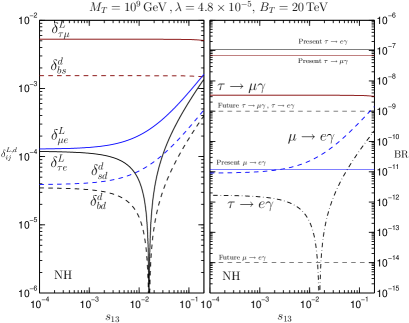
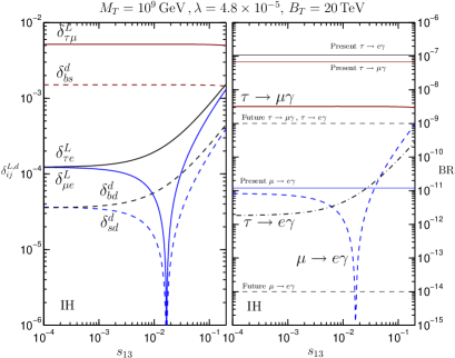
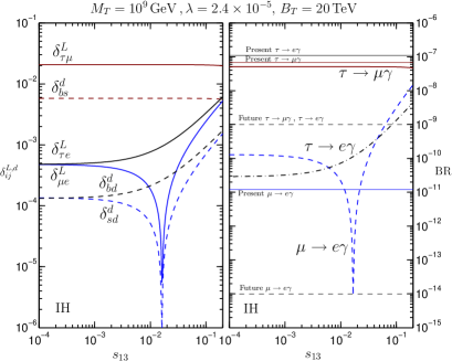
Figure 10: FV parameters $\delta^{L}_{ij},(i,j=e,\mu,\tau)$, $\delta^{d}_{ij},(i,j=d,s,b)$ and ${\rm BR}(\ell_{j}\rightarrow\ell_{i}\gamma)$ as a function of $s_{13}$ for the NH (left upper-panel) and IH (right upper-panel and lower panel). The parameters $M_{T}$, $B_{T}$ and ${\lambda}$ are fixed as indicated on the top of each panel. For each radiative decay, the present upper bound (horizontal solid-lines) and future experimental sensitivity (horizontal dashed-lines) for the BRs are shown.

The behavior of $\delta^{L,d}$ just reflects that of the relevant FV structure ${\bf V}({\bf m}^{D}_{\nu})^{2}{\bf V}^{\dagger}$ in Eq. (5). For example, notice that they scale as $1/{\lambda}^{2}$ outside the cancelation ‘dip’. This figure clearly shows that $\delta^{L}_{\tau\mu},\delta^{d}_{bs}$ are insensitive either to $s_{13}$ or to the type of neutrino spectrum (cf. the upper panels), while $\delta^{L}_{\mu e}(\delta^{d}_{sd})$ gets exchanged with $\delta^{L}_{\tau e}(\delta^{d}_{bd})$ when passing from the NH to the IH case. This latter feature is due to the fact that $\theta_{23}=\pi/4$ and so the flavours $\mu$ and $\tau$ (or $b$ and $s$) are indistinguishable. The relative ratios $\delta^{L}_{\tau\mu}/\delta^{L}_{\mu e},\,\delta^{d}_{bs}/\delta^{d}_{sd}$ and $\delta^{L}_{\tau e}/\delta^{L}_{\mu e},\,\delta^{d}_{bd}/\delta^{d}_{sd}$ just reproduce the absolute values of $R_{23/12}$ and $R_{13/12}$ in Eq. (5), respectively. As we have already deduced from (5), this constant-ratio rule is violated for $s_{13}\approx 0.02$, where $\delta^{L}_{\tau e},\,\delta^{d}_{bd}$ and $\delta^{L}_{\mu e},\,\delta^{d}_{sd}$ are strongly suppressed for the NH and IH spectrum, respectively. All the above peculiarities are common to the related curves of ${\rm BR}(\ell_{j}\to\ell_{i}\gamma)$, plotted on the right of each panel. In particular, the ratios (50) are remarkably reproduced, except for $s_{13}\approx 0.02$ where ${\rm BR}(\tau\to e\gamma)$ and ${\rm BR}(\mu\to e\gamma)$ undergo a sharp suppression for the NH and IH spectrum, respectively. Hence, the point with ${\lambda}=4.8\times 10^{-5}$ and $s_{13}\sim 0.02$ is excluded by the ${\rm BR}(\mu\to e\gamma)$ bound in the NH case, whereas it is allowed in the IH with ${\rm BR}(\tau\to\mu\gamma)\sim 3\times 10^{-9}$, ${\rm BR}(\tau\to e\gamma)\sim{\cal O}(10^{-11})$. The point with ${\lambda}=2.4\times 10^{-5}$ (lower panel) is phenomenologically viable if the neutrinos have IH masses and $s_{13}\sim 0.02$. In such a case, ${\rm BR}(\mu\to e\gamma)\ll 10^{-11}$, ${\rm BR}(\tau\to\mu\gamma)\sim 5\times 10^{-8}$ and ${\rm BR}(\tau\to e\gamma)\sim{\cal O}(10^{-10})$. This is an example where ${\rm BR}(\tau\to\mu\gamma)$ is close to the present bound and $\mu\to e\gamma$ might be unobservable.

In the examples considered above, the size of the $\delta^{d}$’s in each family sector is smaller by a factor of $\sim 3.5$ than the one of the corresponding $\delta^{L}$’s. This results from different compensating effects. Namely, the squark masses are about three times larger than the slepton ones (due to the gluino-induced renormalization effect; see also Fig. 8), while the $({\bf m}_{\tilde{d^{c}}}^{2})_{ij}$ are larger than the $({\bf m}_{\tilde{L}}^{2})_{ij}$ at the messenger scale $M_{T}$ (because of the major strong coupling contribution). In the first example, $\delta^{d}_{bs}~{}\sim 1.5\times 10^{-3}$ (left panel). This is the maximal value attainable by $\delta^{d}_{bs}$ in the allowed parameter space of Fig. 5. To perceive the phenomenological relevance of such $\delta^{d}_{bs}$, we need to confront it with the gluino and squarks masses. Recall that for $B_{T}=20~{}{\rm TeV}$ we got $m_{\tilde{Q}}\sim 900~{}{\rm GeV}$ and $M_{3}\sim 1.3~{}{\rm TeV}$ (see Fig. 8). Then, $\delta^{d}_{bs}\sim 10^{-3}$ is well below the experimental bound posed by the measured ${\rm BR}(b\to s\gamma)$ [60]. The predicted value $\delta^{d}_{sd}\sim 5\times 10^{-4}$ (obtained for $s_{13}=0.2$) also lies below the bound inferred from $K^{0}-\bar{K}^{0}$ mixing [60].

Fig. 11 is aimed to address the dependence of the ratios ${\rm BR}(\tau\to\mu\gamma)/{\rm BR}(\mu\to e\gamma)$ and ${\rm BR}(\tau\to e\gamma)/{\rm BR}(\mu\to e\gamma)$ on $s_{13}$ and the CP-violating phase $\delta$ for a NH (left panel) and IH spectrum (right panel). The results do not depend on the ratio $M_{T}/{\lambda}$ as far as either the quadratic or the quartic terms dominate in the LFV entries ${\bf m}^{2}_{\tilde{L}}$. Regarding the ratio ${\rm BR}(\tau\to\mu\gamma)/{\rm BR}(\mu\to e\gamma)$, it slightly decreases (increases) with increasing $s_{13}$ for $\delta<\pi/2$ ($\delta>\pi/2$).

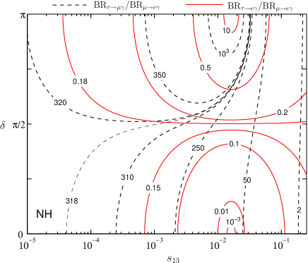
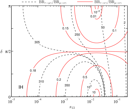
Figure 11: Contours of the ratios ${\rm BR}{(\tau\to\mu\gamma)}/{\rm BR}{(\mu\to e\gamma)}$ (dashed lines) and ${\rm BR}{(\tau\to e\gamma)}/{\rm BR}{(\mu\to e\gamma)}$ (solid lines) in the $(s_{13},\delta)$-plane, for the NH (left panel) and IH (right panel) neutrino mass spectra.

However, this ratio blows up at $s_{13}\sim 0.02$ and $\delta\approx\pi\,(0)$ for the NH (IH) spectrum. The ${\rm BR}(\tau\to e\gamma)/{\rm BR}(\mu\to e\gamma)$ is also sensitive to both $s_{13}$ and $\delta$. In fact, for a given value of $s_{13}$, the increase of this ratio with $\delta$ is quite modest in most of the $s_{13}$ range. Still, for $s_{13}\approx 0.02$, ${\rm BR}(\tau\to e\gamma)/{\rm BR}(\mu\to e\gamma)$ goes to zero (infinity) when $\delta=0\,(\pi)$ for the NH case. Instead, the opposite occurs when the IH pattern is considered since there is an interchange of the roles played by ${\rm BR}(\mu\to e\gamma)$ and ${\rm BR}(\tau\to e\gamma)$ (as already discussed). In short, barring the range around $s_{13}\approx 0.02$, the predictions (50), (7.2) and (62) are not substantially altered when the effects of $\delta\neq 0$ are included.

Finally, we come to a comparative analysis of radiative decays, 3-body decays and $\mu\to e$ conversion in Ti considering the three types of neutrino spectrum. Fig. 12 shows the dependence of the ${\rm BR}$s on ${\lambda}$ for $M_{T}=10^{9}~{}{\rm GeV}$ and $s_{13}=0\,(0.2)$ in the upper (lower) panels, assuming a NH spectrum ($m_{1}=0~{}{\rm eV}$).

For $s_{13}=0$ there is a cancelation dip only in ${\rm BR}(\tau\to\mu\gamma)$ (left panel), ${\rm BR}(\tau\to\mu ee)$ and ${\rm BR}(\tau\to 3\mu)$ (right panel) at ${\lambda}\sim 3.5\times 10^{-6}$, which lies in the (green) region excluded by the negative sparticle search, ${\lambda}\leq 6\times 10^{-6}$ (cf. also Fig. 5: upper panel). This dip originates from the cancelations of the quadratic and quartic terms in ${\bf m}^{2}_{\tilde{L}}$ discussed in Section 5. In ${\rm BR}(\mu\to e\gamma)$ this would take place at a value of ${\lambda}$ smaller by a factor of $\sim(6/78)^{1/2}\sim 0.3$ [see Eq. (5)] and so, would fall into the (grey) non-perturbative range. For $s_{13}=0.2$ the dips are instead present for all the BRs, as we expect on the basis of Eq. (32).

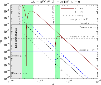
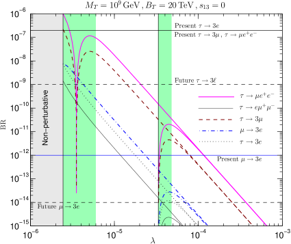
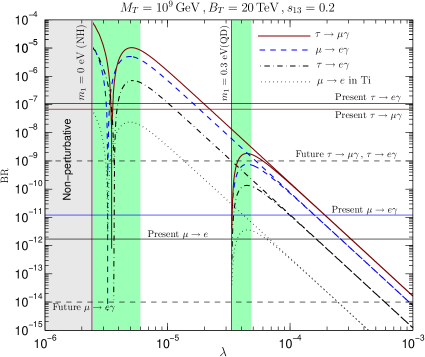
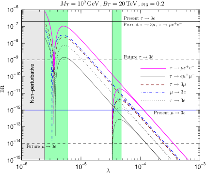
Figure 12: Left panels: branching ratios of the radiative decays $\ell_{j}\rightarrow\ell_{i}\gamma$ and $\mu\rightarrow e$ conversion in Ti, as a function of ${\lambda}$. Right panels: branching ratios of the three-body decays $\ell_{j}\to 3\ell_{i}$ and $\tau\rightarrow\mu ee\,,\,e\mu\mu$. All the results are shown as a function of ${\lambda}$ for $M_{T}=10^{9}~{}{\rm GeV}$ and $B_{T}=20$ TeV taking $s_{13}=0$ (upper plots) and $s_{13}=0.2$ (lower plots). The left (right) vertical line indicates the lower bound on $\lambda$ imposed by requiring perturbativity of the Yukawa couplings ${\bf Y}_{T,S,Z}$ when $m_{1}=0\,(0.3)$ eV [NH (QD) neutrino mass spectrum]. The regions in green (grey) are excluded by the $m_{\tilde{\ell}_{1}}>100$ GeV constraint (perturbativity requirement when $m_{1}=0$ eV).

Outside the cancelation regions, the relative ratios of ${\rm BR}(\ell_{j}\to\ell_{i}\gamma)$ are those announced in Eq. (50) and the ${\rm BR}(\ell_{j}\to\ell_{i}\ell_{k}\ell_{k})$ are correlated with ${\rm BR}(\ell_{j}\to\ell_{i}\gamma)$ according to Eq. (7.2). For comparison, we have also plotted all these ${\rm BR}$s for the case of the QD spectrum with $m_{1}=0.3~{}{\rm eV}$ which can be obtained by ‘continously’ rising the mass $m_{1}$ in the NH case beyond $(\Delta m^{2}_{A})^{1/2}$ [cf. Eq. (19)]. In the QD case the non-perturbative range extends much above the one relative to the NH (grey) so that the perturbativity lower bound on ${\lambda}$ (indicated by the vertical solid line) is larger by about one order of magnitude, ${\lambda}\geq 3\times 10^{-5}$. Notice that a more restrictive lower bound is imposed by sparticle searches (green), ${\lambda}\geq 5\times 10^{-5}$. The cancelations occur at approximately the same ${\lambda}$ (inside the excluded regions) for all the BRs. For ${\lambda}\geq 5\times 10^{-5}$, the curves corresponding to the NH and QD are superimposed and so the two scenarios are not distinguishable [cf. Eqs. (28) and (5)].

Finally, Fig. 12 reveals that, for $M_{T}=10^{9}~{}{\rm GeV}$ and assuming a NH spectrum with $s_{13}\approx 0$, only ${\rm BR}(\mu\to e\gamma),~{}{\rm BR}(\tau\to\mu\gamma)$, ${\rm BR}(\mu\to 3e)$ and ${\rm CR}(\mu\to e;{\rm Ti})$ are within the future experimental sensitivities for $5\times 10^{-5}\lower 3.01385pt\hbox{$\;\stackrel{{\scriptstyle\textstyle<}}{{\sim}}\;$}{\lambda}\lower 3.01385pt\hbox{$\;\stackrel{{\scriptstyle\textstyle<}}{{\sim}}\;$}7\times 10^{-5}$, while if ${\lambda}>7\times 10^{-5}$ only $\mu\to e\gamma$ and ${\rm CR}(\mu\to e;{\rm Ti})$ could be accessible. All the other LFV processes would be undetectable in the allowed ${\lambda}$ range. Then, if for example the MEG experiment [36] detects ${\rm BR}(\mu\to e\gamma)$ at the level of $8\times 10^{-12}$ then ${\rm BR}(\tau\to\mu\gamma)$, ${\rm BR}(\mu\to 3e)$ and ${\rm CR}(\mu\to e;{\rm Ti})$ are expected to be $\sim 2\times 10^{-9}$, $\sim 5\times 10^{-14}$ and $\sim 4\times 10^{-14}$, respectively. The case of the QD spectrum is similar: in the range ${\lambda}\sim(6-7)\times 10^{-5}$ the $\mu e$ LFV decays are observable but ${\rm BR}(\tau\to\mu\gamma)$ is predicted to be $\lower 3.01385pt\hbox{$\;\stackrel{{\scriptstyle\textstyle<}}{{\sim}}\;$}10^{-9}$, and for larger ${\lambda}$ only $\mu\to e\gamma$ and $\mu\to e$ conversion would be visible.

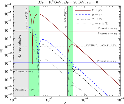
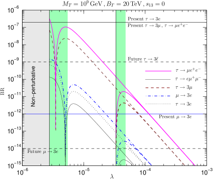
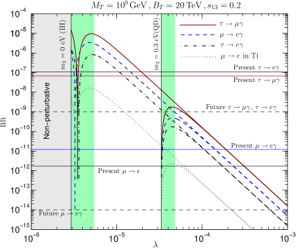
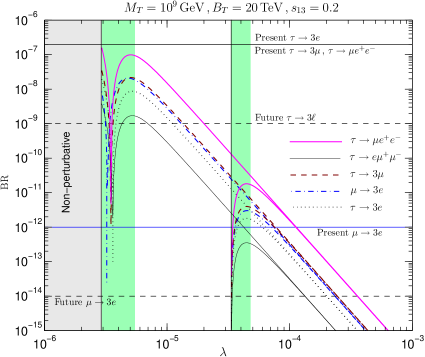
Figure 13: The same as in Fig. 12 for the case of an IH neutrino mass spectrum ($m_{3}=0$ eV). For comparison, the results with $m_{3}=0.3$ eV are also shown.

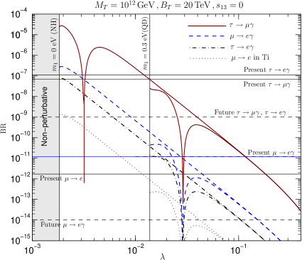
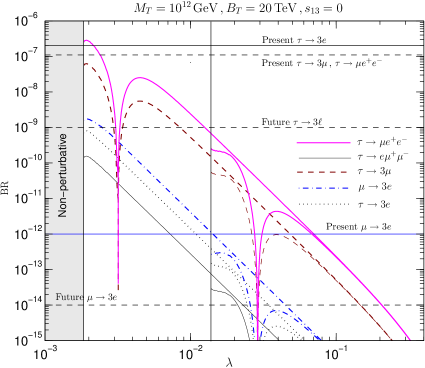
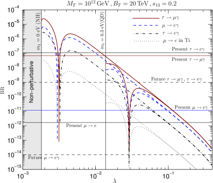
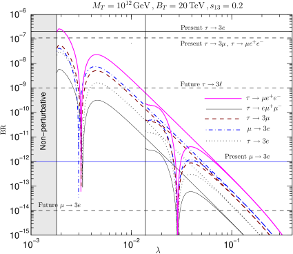
Figure 14: As in Fig. 12 but for $M_{T}=10^{12}~{}{\rm GeV}$.

By switching on $s_{13}$, LFV is enhanced in the $\mu e$ and $\tau e$ sectors, but it is not essentially altered in the $\tau\mu$ sector. As a consequence, the lower bound on ${\lambda}$ imposed by the present limit on ${\rm BR}(\mu\to e\gamma)$ is more restrictive (cf. Fig. 5) and consequently, the ${\rm BR}$s of the $\tau\mu$ sector are penalised. For instance, detecting $\mu\to e\gamma$ with a BR around $8\times 10^{-12}$ would imply the possibility to measure also ${\rm BR}(\mu\to 3e)$ and ${\rm CR}(\mu\to e;{\rm Ti})$ at the level of $5\times 10^{-14}$ and $4\times 10^{-14}$, but ${\rm BR}(\tau\to\mu\gamma)$ would be $\sim 10^{-11}$ (well below the planned future capability). This conclusion holds for both the NH and QD spectrum.

Fig. 13 presents a similar analysis for the IH spectrum with $m_{3}=0~{}{\rm eV}$. For comparison, we also show the QD case which can be obtained by pushing the mass $m_{3}$ to values larger than $(\Delta m^{2}_{A})^{1/2}$ thus recovering a case very similar to the QD one reported in Fig. 12. When $s_{13}=0$ (upper panels) the main difference with the NH case is the fact that all BRs exhibit the suppression dip in the perturbative range (in the $\tau\mu$ sector this takes place for a smaller ${\lambda}$ with respect to the $\mu e$ one). However, due to the choice of $B_{T}$ these dips fall into the (green) range excluded by sparticle searches. Outside these cancelation regions the values of all these ${\rm BR}$s (and the related correlations) are essentially the same as those obtained for the NH case leading to the same phenomenological implications.

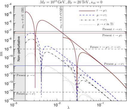
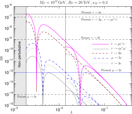
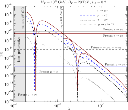
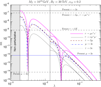
Figure 15: As in Fig. 13 but for $M_{T}=10^{12}~{}{\rm GeV}$.

The IH scenario offers the possibility to reverse the dominance of the $\mu e$ LFV over the $\tau\mu$ LFV. Suppose that the effective SUSY breaking is increased up to $B_{T}\lower 3.01385pt\hbox{$\;\stackrel{{\scriptstyle\textstyle>}}{{\sim}}\;$}70~{}{\rm TeV}$ so that all the sparticle masses are enhanced by a factor of 3.5. Then the ${\rm BR}(\mu\to e\gamma)$ dip would lie in the allowed ${\lambda}$ range and ${\rm BR}(\tau\to\mu\gamma)$ would be brought close to the present bound. As a result, $\mu\to e\gamma$, $\mu\to 3e$ and $\mu\to e$ conversion might be invisible, whereas ${\rm BR}(\tau\to\mu\gamma)\sim 5\times 10^{-8}$ could be measured [perhaps together with ${\rm BR}(\tau\to\mu ee)\sim 5\times 10^{-10}$].

By switching on $s_{13}=0.2$ (lower panels) we find, as for the NH case, that all the LFV processes undergo a dramatic suppression at the same ${\lambda}$ which, however, occurs in the excluded range. Outside this interval, the relative ratios of the ${\rm BR}$s closely follow the predictions (50), (7.2) and (62). In such a case, the planned experimental sensitivities would allow to test only $\mu\to e\gamma$, $\mu\to 3e$ and $\mu\to e$ conversion.

Figs. 14 and 15 contain the results of a similar analysis performed by taking $M_{T}=10^{12}~{}{\rm GeV}$ for the NH and IH spectrum, respectively. The increasing of $M_{T}$ implies an overall decreasing of all the BRs due to a heavier sparticle spectrum (cf. Fig. 8) with respect to the case with $M_{T}=10^{9}~{}{\rm GeV}$. We again find that for any ${\lambda}$ (barring the cancelation ranges) the several BRs are correlated according to the model-independent predictions contained in Eqs. (50), (7.2) and (62). The features of the cancelation dips are those discussed in Section 5 and already encountered for smaller $M_{T}$. Consider the NH case (Fig. 14). At $s_{13}=0$ and ${\lambda}$ within $(3-4)\times 10^{-2}$, $\mu\to e\gamma,\,\tau\to\mu\gamma$, $\mu\to 3e$ and $\mu\to e$ conversion are in the reach of the future experiments in both the NH and QD cases. From ${\lambda}\sim 4\times 10^{-2}$ up to $1.5\times 10^{-1}$ only $\mu\to e\gamma$ and $\mu\to e$ conversion could be detected. For $s_{13}=0.2$ and ${\lambda}\geq 0.1$ only $\mu\to e\gamma$, $\mu\to 3e$ and $\mu\to e$ conversion are accessible. We arrive at similar conclusions observing the case of IH spectrum displayed in Fig. 15: the $\mu e$ sector is more favoured with respect to the $\tau\mu$ sector, where only the $\tau\to\mu\gamma$ decay could be detected as far as $s_{13}\approx 0$. However, this conclusion could be contradicted for larger $B_{T}$ and $s_{13}=0$. Consider $B_{T}\lower 3.01385pt\hbox{$\;\stackrel{{\scriptstyle\textstyle>}}{{\sim}}\;$}50~{}{\rm TeV}$ so that the sparticle spectrum increases by a factor of 2.5. Then, in the suppression dips of the $\mu e$ LVF processes (see upper panels in Fig. 15), ${\rm BR}(\tau\to\mu\gamma)$ would be close to the present bound and ${\rm BR}(\tau\to\mu ee)\sim 10^{-9}$. Therefore, the future detection of both $\tau\to\mu\gamma$ and $\tau\to\mu ee$, together with a slepton and squark spectrum in the range $400-650~{}{\rm GeV}$ and $1.8-2.5~{}{\rm TeV}$, respectively, would point to a IH neutrino masses and $s_{13}\approx 0$.

8 Summary and Conclusions

The future perspectives to detect signals of new physics mostly rely on the observation of sparticles at the LHC or LFV decays at e g. the B-factories [38], the incoming MEG experiment [36], the Super Flavour factory [61] or the PRISM/PRIME experiment at J-PARC [46]. It is, therefore, extremely important to motivate and suggest theoretical scenarios which can be tested in more than one direction. In this paper we have presented and discussed in detail a supersymmetric $SU(5)$ version of the triplet seesaw mechanism in which the triplet are messengers of both $L$ and SUSY breaking. The key-points of our model can be outlined as follows:

• The tree-level exchange of the triplets $T$ generates neutrino masses, so flavour violation is induced also in the lepton sector of the SM, as required by the observation of neutrino oscillations. All the LFV effects are parameterized by a single flavour structure ${\bf Y}_{T}$;

• The quantum-level exchange of the 15-states $T,\,S$ and $Z$ generates all the SSB mass parameters of the MSSM via gauge and Yukawa interactions. Their mass scale is determined by the effective SUSY breaking scale $B_{T}$. Flavour violation is induced in the mass matrices ${\bf m}^{2}_{\tilde{L}}$ and ${\bf m}^{2}_{\tilde{d^{c}}}$, and in the trilinear terms ${\bf A}_{e}$ and ${\bf A}_{d}$, by the Yukawa couplings ${\bf Y}_{T}$ (and, according to the $SU(5)$ relation (12), also by ${\bf Y}_{S}$ and ${\bf Y}_{Z}$). Therefore, the flavour structure of the SSB parameters is provided by ${\bf Y}_{T}$ or, according to Eq. (18), by the low-energy neutrino parameters.

• The number of free parameters is three: the triplet mass $M_{T}$, the effective SUSY breaking scale $B_{T}$ and the unflavoured coupling constant ${\lambda}$.

These aspects make the present scenario highly predictive since it relates neutrino masses and mixing, sparticle and Higgs spectra, lepton and quark flavour violation in the sfermion masses and electroweak symmetry breaking. We have performed a complete analysis of the parameter space spanned by $M_{T}$, $B_{T}$ and ${\lambda}$ taking into account the present experimental constraints on the above physical observables (see Figs. 5 and 6). This has demonstrated that there is a region in the parameter space where our framework is compatible with experiment. In particular, despite the very constrained structure of our SSB mass parameters, EWSB can be radiatively realized analogously to the conventional MSSM case. Our predictions allow us to further test the allowed parameter space as follows:

• Regarding the MSSM sparticle spectrum, we predict that the gluino is the heaviest sparticle while, in most of the parameter space, $\tilde{\ell}_{1}$ is the lightest. However, the gravitino is lighter than the MSSM sparticles. For instance, if $B_{T}=20$ TeV, the squark and slepton masses lie in the ranges $800-950$ GeV and $100-300$ GeV, respectively. The chargino masses are $m_{\tilde{\chi}^{\pm}_{1}}\sim 320$ GeV and $m_{\tilde{\chi}^{\pm}_{2}}\sim 450-550$ GeV. Moreover, $m_{\tilde{\chi}^{0}_{1}}\sim 190$ GeV, $m_{\tilde{\chi}^{0}_{2}}\approx m_{\tilde{\chi}^{\pm}_{1}}$ and $m_{\tilde{\chi}^{0}_{3,4}}\approx m_{\tilde{\chi}^{\pm}_{2}}$. These mass ranges are within the discovery reach of the LHC. Increasing the parameter $B_{T}$ implies a linearly heavier spectrum. The measurement of only a few sparticle masses will provide a hint on the value of the effective SUSY breaking scale $B_{T}$ and a test of the correlation pattern shown in Fig. 8.

  The mass range of the electroweak sparticles implies that the SUSY contribution to the muon anomalous magnetic moment $\delta a_{\mu}$ never exceeds the maximum value of the interval (39). Moreover, since $\delta a_{\mu}>0$, the discrepancy between the experimental determination and SM prediction is alleviated in our model.

• The Higgs sector is characterized by a decoupling regime with a light SM-like Higgs boson ($h$) and the three heavy states ($H,A$ and $H^{\pm}$) with mass $m_{H,A,H^{\pm}}\approx 450-550$ GeV (again, for $B_{T}=20$ TeV). These masses increase almost linearly with $B_{T}$.

• We have considered several LFV processes: $\mu\to eX$, $\mu\to e$ conversion in nuclei, $\tau\to eY$ and $\tau\to\mu Y$ $(X=\gamma,ee$, $Y=\gamma,ee,\mu\mu)$. Our framework is characterized by peculiar LFV and QFV patterns [intimately related to each other; see Eq. (5)], which are mostly determined by low-energy neutrino masses and mixing. The size of QFV, when confronted with the coloured sparticle spectrum, is well below the present phenomenological bounds extracted from $b\to s\gamma$ and $K^{0}-\bar{K}^{0}$ mixing, etc. Therefore, QFV processes do not constrain our parameter space.

Concerning LFV, we stress that strict predictions have been obtained for the relative branching ratios of the radiative $\ell_{j}\to\ell_{i}\gamma$ [see Eq. (50)] and 3-body $\ell_{j}\to\ell_{i}\ell_{k}\ell_{k}$ decays [see Eq. (62)]. The latter, as well as $\mu\to e$ conversion in Ti, are also correlated with the radiative decays as shown in Eq. (7.2). All these results are model-independent in the sense that they do not depend on $M_{T}$, $B_{T}$ or ${\lambda}$ (they are given only in terms of the low-energy neutrino observables). If the present bound on ${\rm BR}(\mu\to e\gamma)$ is saturated, the branching ratios of the remaining LFV processes are predicted as shown in Table 2, where the three types of neutrino spectrum have been considered. The experimental signatures of our scenario crucially depend on the value of the lepton mixing angle $\theta_{13}$:

Tiny $\bm{\theta_{13}}$: The analysis has shown that, in the allowed parameter space, the future experimental sensitivity will allow to measure at most ${\rm BR}(\mu\to e\gamma)$, ${\rm BR}(\mu\to 3e)$, ${\rm BR}(\tau\to\mu\gamma)$ and CR($\mu\to e\,$ Ti) according to the relations (50) and (7.2). In particular, being ${\rm BR}(\tau\to\mu\gamma)/{\rm BR}(\mu\to e\gamma)\sim 300$, ${\rm BR}(\tau\to\mu\gamma)$ is expected not to exceed $3\times 10^{-9}$, irrespective of the type of neutrino spectrum. All the decays $\tau\to\ell_{i}\ell_{k}\ell_{k}$ would have ${\rm BR}<\mathcal{O}(10^{-11})$.

Sizeable $\bm{\theta_{13}}$: If $s_{13}$ is close to the upper bound (23), the $\tau\mu$ sector is hardly accessible and only the decays $\mu\to e\gamma$, $\mu\to 3e$ and $\mu\to e$ conversion in Ti can be observed in the future. This conclusion holds for the NH, IH and QD neutrino spectra. For instance, if the MEG experiment measures ${\rm BR}(\mu\to e\gamma)\sim 8\times 10^{-12}$, then ${\rm BR}(\mu\to 3e)$ and CR($\mu\to e\,$ Ti) are expected to be $\sim 5\times 10^{-14}$ and $\sim 4\times 10^{-14}$. The latter is in the reach of the PRISM/PRIME sensitivity. Values of $s_{13}\sim\mathcal{O}(10^{-1})$ will be explored soon by several neutrino experiments like MINOS, OPERA and Double Chooz [62].

Deviations to this very specific model-independent pattern occur when $({{\bf m}^{2}_{\tilde{L}}})_{ij}$ cancel (see discussion in Section 5). This can be the case if $s_{13}\approx 0.02(-0.02)$ and the neutrino spectrum is IH (NH). Then, all the $\mu e$ LFV processes might be invisible and $\tau\to\mu\gamma$ detected with a BR close to the present bound (taking $B_{T}=20$ TeV). Moreover, $\tau\to\mu ee$ would be $\mathcal{O}(10^{-9}-10^{-10})$ and the remaining $\tau$ decays below $10^{-10}$. Notice that, increasing $B_{T}$ the BRs are suppressed since they scale as $1/B_{T}^{4}$. This specific value of $s_{13}$ is in the sensitivity range of Neutrino Factories [63].

Alternatively, $({{\bf m}^{2}_{\tilde{L}}})_{\mu e}$ could be vanishing because of a cancelation between the quadratic and quartic Yukawa contributions [see Eq. (5)]. For the IH case, if $B_{T}\lower 3.01385pt\hbox{$\;\stackrel{{\scriptstyle\textstyle>}}{{\sim}}\;$}50\,$TeV and $s_{13}$ is very small, all the $\mu e$ LFV processes would be strongly suppressed whereas the $\tau\mu$ sector would be favoured with ${\rm BR}(\tau\to\mu\gamma)\sim 5\times 10^{-8}$ and ${\rm BR}(\tau\to\mu ee)\sim\times 10^{-9}$. This scenario is correlated with a slepton and squark spectrum in the ranges 400-650 GeV (in the limit of the LHC detection capabilities) and above $\sim 2$ TeV (within the LHC reach), respectively.

Given the increasing interest on the problem of finding a possible relation between leptogenesis [64] and low-energy neutrino physics [65], we would like to comment on this issue in the framework of our work. Within the present version of the supersymmetric triplet seesaw mechanism, leptogenesis can be realized by considering that the soft bilinear term $B_{T}$ produces a mass splitting between $T$ and $\bar{T}$, leading to resonant leptogenesis [66]. For this to work, $B_{T}$ must be around the electroweak scale. In our case, since $B_{T}\lower 3.01385pt\hbox{$\;\stackrel{{\scriptstyle\textstyle>}}{{\sim}}\;$}20$ TeV, the BAU turns out to be too small. Still, leptogenesis could be made effective either by adding an additional pair of triplets [14] or by including heavy singlet neutrinos [67]. The former case would imply the appearance of one more flavour source ${\bf Y}^{\prime}_{T}$ which, depending on its size, could have some impact in the predictions of our framework. Instead, we would like to comment on the second possibility which requires heavy neutrino singlets (with mass $M_{N}$) coupled to the lepton doublets through the Yukawa couplings ${\bf Y}_{N}$. To maintain the predictions made along this work we must require that the singlet contribution to neutrino masses is much smaller then the one generated by the triplet i.e., ${\bf Y}_{N}^{2}\ll{\lambda}{\bf Y}_{T}M_{N}/M_{T}$. Moreover, ${\bf Y}_{N}\ll{\bf Y}_{T}$ is also required to suppress LFV arising in the SSB parameters from the singlet exchange at the quantum level (notice that the neutrino singlets could couple to the spurion field $X$). For the purpose of leptogenesis, two different situations can be envisaged: $M_{N}>M_{T}$ or $M_{N}<M_{T}$. In the former case, the $CP$-asymmetry generated through the decay of the triplets into two leptons is directly proportional to ${\bf Y}_{N}^{2}/M_{N}$ [67], so it turns out to be very tiny (${\bf Y}_{N}^{2}\ll{\lambda}{\bf Y}_{T}M_{N}/M_{T}$). On the contrary, if $M_{N}<M_{T}$ the $CP$-asymmetry is weakly sensitive to $Y_{N}$ [67], therefore a viable value for the BAU can be achieved.

We conclude our discussion by remarking that our scenario is not only extremely predictive but it can also be tested in view of the present and future programmes of LFV and neutrino oscillation experiments.

Acknowledgments: We thank A. Brignole for valuable comments and suggestions and T. Hambye for useful discussions. The work of F.R.J. is supported by Fundação para a Ciência e a Tecnologia (FCT, Portugal) under the grant SFRH/BPD/14473/2003, INFN and PRIN Fisica Astroparticellare (MIUR). The work of A. R.  is partially supported by the project EU MRTN-CT-2004-503369.

Appendix A-Extracting the SSB terms from wave function renormalization

In this Appendix we derive the general expressions for the soft supersymmetry breaking scalar masses, the bilinear and trilinear couplings at the messenger scale $M$. We employ a generalization of the method suggested in Ref. [30] and subsequently presented in Ref. [31]. Consider the case in which the scales of SUSY breaking and its mediation to the observable sector are determined by the vev of the auxiliary and scalar components of a chiral singlet superfield $X$, $\langle X\rangle=M+\theta^{2}F$ (in the following $M$ is taken to be real and $|F|<M^{2}$, for consistency of the method). The leading contributions (at lowest order in $F$) to the SSB terms arise from $X$-dependent wave-function renormalizations of the chiral superfields ${\bf Z}_{\cal Q}$. The effective Lagrangian reads

$${\cal L}=\int{\rm d}^{4}\theta{\cal Q}^{\dagger}_{a}{\bf Z}_{\cal Q}(X,X^{\dagger})^{a}_{b}{\cal Q}^{b}+\left[\int{\rm d}^{2}\theta(\mu_{ab}{\cal Q}^{a}{\cal Q}^{b}+f_{abc}{\cal Q}^{a}{\cal Q}^{b}{\cal Q}^{c})+{\rm h.c.}\right]\,,$$ (A-1)

where $\mu_{ab}$ and $f_{abc}$ are superpotential mass parameters and dimensionless coupling constants, respectively. The wave-function renormalization ${\bf Z}_{\cal Q}$ is a hermitian matrix which depends on $|X|=\sqrt{XX^{\dagger}}$. Its $\theta$-expansion at $X=\langle X\rangle$ is given by

$$\left.{\bf Z}_{\cal Q}(|X|)\right|_{X=\langle X\rangle}={\bf Z}_{\cal Q}(M)+\frac{1}{2}\frac{\partial{\bf Z}_{\cal Q}}{\partial{\rm ln}M}\left(\theta^{2}\frac{F}{M}+\bar{\theta}^{2}\frac{F^{\dagger}}{M}\right)+\frac{1}{4}\frac{\partial^{2}{\bf Z}_{\cal Q}}{\partial{\rm ln}M^{2}}\theta^{2}\bar{\theta}^{2}\frac{FF^{\dagger}}{M^{2}}\,.$$ (A-2)

After expressing Eq. (A-1) in terms of the canonically normalized superfields ${\cal Q}^{{}^{\prime}}$ as

$${\cal Q}=\left(1+\frac{{\bf Z}^{-1}_{\cal Q}}{2}\frac{\partial{\bf Z}_{\cal Q}}{\partial M}\theta^{2}F\right){\bf Z}^{-1/2}_{\cal Q}{\cal Q}^{{}^{\prime}}\,,$$ (A-3)

we can extract the SSB masses for the scalar component of ${\cal Q}$ from the quartic terms $\theta^{2}\bar{\theta}^{2}$ in the first integral and the SSB bilinear and trilinear couplings from the quadratic terms $\theta^{2}$ in the second and third integral, respectively

$${\bf m}^{2}_{\tilde{{\cal Q}}} = -\frac{1}{4}{\bf Z}^{-1/2}_{\cal Q}\left(\frac{\partial^{2}{\bf Z}_{\cal Q}}{\partial{\rm ln}M^{2}}-\frac{\partial{\bf Z}_{\cal Q}}{\partial{\rm ln}M}{\bf Z}^{-1}_{\cal Q}\frac{\partial{\bf Z}_{\cal Q}}{\partial{\rm ln}M}\right){\bf Z}^{-1/2}_{\cal Q}\frac{FF^{\dagger}}{M^{2}},$$

$${\bf A}_{abc} = \frac{1}{2}\left[f_{a^{{}^{\prime}}bc}\left({\bf Z}^{-1/2}_{\cal Q}\frac{\partial{\bf Z}_{\cal Q}}{\partial{\rm ln}M}{\bf Z}^{-1/2}_{\cal Q}\right)^{a^{{}^{\prime}}}_{a}+f_{ab^{{}^{\prime}}c}\left({\bf Z}^{-1/2}_{\cal Q}\frac{\partial{\bf Z}_{\cal Q}}{\partial{\rm ln}M}{\bf Z}^{-1/2}_{\cal Q}\right)^{b^{{}^{\prime}}}_{b}\right.$$

$$\left.+f_{abc^{{}^{\prime}}}\left({\bf Z}^{-1/2}_{\cal Q}\frac{\partial{\bf Z}_{\cal Q}}{\partial{\rm ln}M}{\bf Z}^{-1/2}_{\cal Q}\right)^{c^{{}^{\prime}}}_{c}\right]\frac{F}{M},$$

$$B_{ab} = \frac{1}{2}\left[\mu_{a^{{}^{\prime}}b}\left({\bf Z}^{-1/2}_{\cal Q}\frac{\partial{\bf Z}_{\cal Q}}{\partial{\rm ln}M}{\bf Z}^{-1/2}_{\cal Q}\right)^{a^{{}^{\prime}}}_{a}+\mu_{ab^{{}^{\prime}}}\left({\bf Z}^{-1/2}_{\cal Q}\frac{\partial{\bf Z}_{\cal Q}}{\partial{\rm ln}M}{\bf Z}^{-1/2}_{\cal Q}\right)^{b^{{}^{\prime}}}_{b}\right].$$ (A-4)

In order to find the explicit expressions for the SSB parameters at an energy scale $\mu$ we recall that the $\mu$-dependence of ${\bf Z}_{\cal Q}$ is expressed by the RG equation:

$$\left\{{\bf Z}^{-1/2}_{\cal Q},\frac{{\rm d}{\bf Z}^{1/2}_{\cal Q}}{{\rm d}t}\right\}=\bm{\gamma}_{\cal Q}\,,$$ (A-5)

where $t={\rm ln}\mu$ and $\bm{\gamma}_{\cal Q}$ is the matrix of anomalous dimension. By defining ${\bf Z}^{1/2}_{\cal Q}=1+\delta{\bf Z}^{1/2}_{\cal Q}$, where $\delta{\bf Z}^{1/2}_{\cal Q}$ encodes the quantum corrections, Eq. (A-5) reads

$$\frac{{\rm d}\delta{\bf Z}^{1/2}_{\cal Q}}{{\rm dt}}=\frac{\bm{\gamma}_{\cal Q}}{2}+\left\{\delta{\bf Z}^{1/2}_{\cal Q},\frac{\bm{\gamma}_{\cal Q}}{4}\right\}\,,$$ (A-6)

at the lowest order. By following the procedure outlined in Ref. [31], we have to formally integrate the above equation to obtain $\delta{\bf Z}^{1/2}_{\cal Q}$ in terms of the anomalous dimension. Afterwards, the solution can be plugged into the expressions (A-4) to extract the SSB terms. For the sake of brevity, we do not report all the intermediate steps (which can be easily performed) and, instead, give the final expressions at $\mu=M$:

$${\bf m}^{2}_{\tilde{{\cal Q}}} = -\frac{1}{4}\left[\frac{{\rm d}\Delta\bm{\gamma}_{\cal Q}(M)}{{\rm d{\rm ln}M}}-\left(\Delta\frac{{\rm d}}{{\rm d}{\rm ln}M}\right)\bm{\gamma}_{{\cal Q}}^{<}(M)\right]\frac{FF^{\dagger}}{M^{2}},$$

$$A_{abc} = \frac{1}{2}\left[f_{a^{{}^{\prime}}bc}\Delta\bm{\gamma}_{\cal Q}(M)^{a^{{}^{\prime}}}_{a}+f_{ab^{{}^{\prime}}c}\Delta\bm{\gamma}_{\cal Q}(M)^{b^{{}^{\prime}}}_{b}+f_{abc^{{}^{\prime}}}\Delta\bm{\gamma}_{\cal Q}(M)^{c^{{}^{\prime}}}_{c}\right]\frac{F}{M},$$

$$B_{ab} = \frac{1}{2}\left[\mu_{a^{{}^{\prime}}b}\Delta\bm{\gamma}_{\cal Q}(M)^{a^{{}^{\prime}}}_{a}+\mu_{ab^{{}^{\prime}}}\Delta\bm{\gamma}_{\cal Q}(M)^{b^{{}^{\prime}}}_{b}\right]\frac{F}{M}$$ (A-7)

where $\bm{\gamma}_{{\cal Q}}^{>}(M)$ [$\bm{\gamma}_{{\cal Q}}^{<}(M)$] is the anomalous dimension above (below) the mass scale $M$, $\Delta\bm{\gamma}_{\cal Q}(M)\equiv\bm{\gamma}_{{\cal Q}}^{>}(M)-\bm{\gamma}_{{\cal Q}}^{<}(M)$ and $(\Delta\frac{{\rm d}}{{\rm d}{\rm ln}M})\bm{\gamma}_{{\cal Q}}^{<}(M)$ means considering the difference of the beta-functions of the couplings contained in $\bm{\gamma}_{{\cal Q}}^{<}(M)$ above and below $M$. Notice that our result (Appendix A-Extracting the SSB terms from wave function renormalization) for ${\bf m}^{2}_{\tilde{{\cal Q}}}$ differs from the one obtained in Ref. [31] because an extra term proportional to the commutator $[\bm{\gamma}_{{\cal Q}}^{>},\bm{\gamma}_{{\cal Q}}^{<}]$ appears in that work, which is manifestly inconsistent for a hermitian quantity such as ${\bf m}^{2}_{\tilde{{\cal Q}}}$. We believe that the appearance of such a commutator is due to the improper definition of the RG equation for ${\bf Z}_{\cal Q}$ given in Eq. (3.5) of Ref. [31].

In the following, we provide the explicit expressions for the relevant anomalous dimensions needed to extract the SSB parameters from Eq. (Appendix A-Extracting the SSB terms from wave function renormalization) in our specific framework. The anomalous dimensions below the scale $M$ are:

$$16\pi^{2}\bm{\gamma}_{L}^{<} = -\left[2{\bf Y}^{\dagger}_{e}{\bf Y}_{e}-4\left(\frac{3}{20}g^{2}_{1}+\frac{3}{4}g^{2}_{2}\right)\right],$$

$$16\pi^{2}\bm{\gamma}_{e^{c}}^{<} = -\left[4{\bf Y}_{e}{\bf Y}^{\dagger}_{e}-\frac{12}{5}g^{2}_{1}\right],$$

$$16\pi^{2}\bm{\gamma}_{Q}^{<} = -\left[2{\bf Y}^{\dagger}_{d}{\bf Y}_{d}+2{\bf Y}^{\dagger}_{u}{\bf Y}_{u}-4\left(\frac{1}{60}g^{2}_{1}+\frac{3}{4}g^{2}_{2}+\frac{4}{3}g^{2}_{3}\right)\right],$$

$$16\pi^{2}\bm{\gamma}_{d^{c}}^{<} = -\left[4{\bf Y}_{d}{\bf Y}^{\dagger}_{d}-4\left(\frac{1}{15}g^{2}_{1}+\frac{4}{3}g^{2}_{3}\right)\right],$$

$$16\pi^{2}\bm{\gamma}_{u^{c}}^{<} = -\left[4{\bf Y}_{u}{\bf Y}^{\dagger}_{u}-4\left(\frac{4}{15}g^{2}_{1}+\frac{4}{3}g^{2}_{3}\right)\right],$$

$$16\pi^{2}\bm{\gamma}_{H_{1}}^{<} = -\left[2{\rm Tr}({\bf Y}^{\dagger}_{e}{\bf Y}_{e}+3{\bf Y}^{\dagger}_{d}{\bf Y}_{d})-4\left(\frac{3}{20}g^{2}_{1}+\frac{3}{4}g^{2}_{2}\right)\right],$$

$$16\pi^{2}\bm{\gamma}_{H_{2}}^{<} = -\left[6{\rm Tr}({\bf Y}^{\dagger}_{u}{\bf Y}_{u})-4\left(\frac{3}{20}g^{2}_{1}+\frac{3}{4}g^{2}_{2}\right)\right].$$ (A-8)

The differences $\Delta\bm{\gamma}_{{\cal Q}}(M)$ are instead the following:

$$16\pi^{2}\Delta\bm{\gamma}_{L} = -6\left({\bf Y}^{\dagger}_{T}{\bf Y}_{T}+{\bf Y}^{\dagger}_{Z}{\bf Y}_{Z}\right),$$

$$16\pi^{2}\Delta\bm{\gamma}_{d^{c}} = -4\left({\bf Y}_{Z}{\bf Y}^{\dagger}_{Z}+2{\bf Y}_{S}{\bf Y}^{\dagger}_{S}\right),$$

$$16\pi^{2}\Delta\bm{\gamma}_{H_{2}} = -6|{\lambda}|^{2},$$

$$16\pi^{2}\Delta\bm{\gamma}_{{\cal F}} = 0,~{}~{}~{}~{}~{}~{}~{}~{}{\cal F}=e^{c},Q,u^{c},H_{1}.$$ (A-9)

Regarding the expressions for the RG equations at one loop in the MSSM framework with the $(15+\overline{15})$ $SU(5)$ representation we refer to Ref. [9]. Finally, we obtain the explicit formulas given in Eqs. (16) and (4).

Appendix B-Coefficients of the $\bm{\ell_{j}\ell_{i}Z}$ operators

In this Appendix we compute the coefficients $A^{L,R}$ of the monopole operators

$$g_{Z}(A^{L}_{ji}\bar{\ell}_{i}\bar{\sigma}^{\mu}\ell_{j}+A^{R}_{ji}{\ell}^{c}_{i}{\sigma}^{\mu}\bar{\ell}^{c}_{j}+{\rm h.c.})Z_{\mu}\;\;,\;\;A^{L(R)}_{ji}=A^{L(R),c}_{ji}+A^{L(R),n}_{ji}$$ (B-1)

where $g_{Z}=g_{2}/c_{W}$ ($c_{W}=\cos{\theta_{W}}$, $\theta_{W}$ is the weak mixing angle) and $A^{L(R),c}$ [$A^{L(R),n}$] stand for the contributions from the chargino/sneutrino [neutralino/charged-slepton] loop diagrams. The two-component spinor notation is used such that, for example, $\ell_{i}(\bar{\ell}^{c}_{i})$ is the left-handed (right-handed) component of the lepton $i$ field $(i=e,\mu,\tau)$. Different one-loop results for such coefficients have been presented in the literature. For instance, the authors of Ref. [11] provided an all-order calculation in the electroweak breaking effects, while the authors of Ref. [56] performed a lowest-order calculation. We found dramatic numerical discrepancies between the two aforementioned results, which cannot be ascribed to the approximation used in Ref. [56]. Moreover, the authors of Ref. [59] have recently re-evaluated the contributions to $A^{L,R}$ and claimed to have found additional contributions disregarded in Ref. [11]. We have independently performed the all-order computation to compare with the previous results and to clarify this issue. The notation of Ref. [11] has been adopted to define the mass eigenstates of the charged sleptons $\tilde{\ell}_{X},(X=1,\ldots 6)$ , sneutrinos $\tilde{\nu}_{X},(X=1,\ldots 3)$, charginos $\tilde{\chi}^{-}_{A},(A=1,2)$ and neutralinos $\tilde{\chi}^{0}_{A},(A=1,\ldots 4)$. The corresponding (unitary) mixing matrices are denoted by $U^{\ell}_{Xi},U^{\nu}_{Xi},(O_{L})_{A\alpha},(O_{R})_{A\alpha}$ and $(O_{N})_{A\beta}$ (where $\alpha(\beta)$ is the current-basis index for charged or neutral gauginos/higgsinos). The relevant interactions of sleptons/leptons with charginos and neutralinos are:

$${\cal L}=\bar{\ell}_{i}C^{R}_{iAX}\tilde{\nu}_{X}\bar{\tilde{\chi}}^{+}_{A}+{e}^{c}_{i}C^{L}_{iAX}\tilde{\nu}_{X}\tilde{\chi}^{-}_{A}+\bar{\ell}_{i}N^{R}_{iAX}\tilde{\ell}_{X}\bar{\tilde{\chi}}^{0}_{A}+{e}^{c}_{i}N^{L}_{iAX}\tilde{\ell}^{c}_{X}\tilde{\chi}^{0}_{A}+{\rm h.c.},$$ (B-2)

where

$$C^{R}_{iAX}=-g_{2}(O_{R})_{A1}U^{\nu}_{Xi}\quad,\quad C^{L}_{iAX}=g_{2}\frac{m_{\ell_{i}}}{\sqrt{2}m_{W}\cos\beta}(O_{L})_{A2}U^{\nu}_{Xi},$$

$$N^{R}_{iAX}=-\frac{g_{2}}{\sqrt{2}}\left\{-[(O_{N})_{A2}+(O_{N})_{A1}\tan\theta_{W}]U^{\ell}_{Xi}+\frac{m_{\ell_{i}}}{m_{W}\cos\beta}(O_{N})_{A3}U^{\ell}_{X(i+3)}\right\},$$

$$N^{L}_{iAX}=-\frac{g_{2}}{\sqrt{2}}\left[2(O_{N})_{A1}\tan\theta_{W}U^{\ell}_{X(i+3)}+\frac{m_{\ell_{i}}}{m_{W}\cos\beta}(O_{N})_{A3}U^{\ell}_{X(i+3)}\right]\,.$$ (B-3)

The interactions of charginos and neutralinos with the $Z$ boson are the following:

$${\cal L}=-g_{Z}\left(\overline{\tilde{\chi}^{+}}_{A}\bar{\sigma}^{\mu}\tilde{\chi}^{+}_{B}R_{AB}-\overline{\tilde{\chi}^{-}}_{A}\bar{\sigma}^{\mu}\tilde{\chi}^{-}_{B}L_{AB}+\overline{\tilde{\chi}^{0}}_{A}\bar{\sigma}^{\mu}\tilde{\chi}^{0}_{B}N_{AB}\right)Z_{\mu},$$ (B-4)

where

$$R_{AB}=\left[c^{2}_{\theta_{W}}(O_{R}^{\ast})_{A1}(O_{R})_{B1}+\left(\frac{1}{2}-s^{2}_{\theta_{W}}\right)(O_{R}^{\ast})_{A2}(O_{R})_{B2}\right]\quad,\quad L_{AB}=R^{\ast}_{AB}|_{R\rightarrow L},$$

$$N_{AB}=\frac{1}{2}\left[(O_{N}^{\ast})_{A3}(O_{N})_{B3}-(O_{N}^{\ast})_{A4}(O_{N})_{B4}\right]$$ (B-5)

The chargino contributions are:

$$A^{L,c}_{ji} \!\!=\!\! \frac{C^{R}_{iBX}C^{R*}_{jAX}}{16\pi^{2}}\left[R^{\ast}_{AB}\frac{F(x_{\tilde{\chi}_{A}\tilde{\nu}_{X}},x_{\tilde{\chi}_{B}\tilde{\nu}_{X}})+{\rm ln}\frac{\mu^{2}}{M_{A}^{2}}}{2}-\frac{M_{\tilde{\chi}_{A}}M_{\tilde{\chi}_{B}}}{m^{2}_{\tilde{\nu}_{X}}}L_{AB}G(x_{\tilde{\chi}_{A}\tilde{\nu}_{X}},x_{\tilde{\chi}_{B}\tilde{\nu}_{X}})\right.$$ (B-6)

$$\left.-\delta_{AB}\left(\frac{1}{2}-Z^{\ell}_{L}\right)\frac{H(x_{\tilde{\chi}_{A}\tilde{\nu}_{X}})+{\rm ln}\frac{\mu^{2}}{M_{A}^{2}}}{2}\right],$$

$$A^{R,c}_{ji} \!\!=\!\! A^{L,c}_{ji}|_{L\leftrightarrow R},$$ (B-7)

here $A,B=1,2$, $\,X=1,2,3$ and $Z^{\ell}_{L(R)}=T^{3}_{\ell_{L(R)}}-Q_{\ell}s^{2}_{\theta_{W}}$ ($T^{3}_{\ell_{L}}=-\frac{1}{2},T^{3}_{\ell_{R}}=0$ and $Q_{\ell}=-1$). (A summation over repeated indices is understood.) In the above equations the first and second terms come from the diagrams in which the $Z$ boson line is attached to the chargino line, the third one where it is attached to the sneutrino and the fourth term comes from the wave function renormalization. For completeness, we have also displayed the terms proportional to ${\rm ln}(\mu^{2}/M_{A}^{2})$ in Eq. (B-6), coming from the divergent diagrams, where $\mu$ is the renormalization scale. Obviously, such terms cancel out. As for the argument of the loop functions we have adopted the convention $x_{ab}=m^{2}_{a}/m^{2}_{b}$, then e.g. $x_{\tilde{\chi}_{A}\tilde{\nu}_{X}}=M^{2}_{\tilde{\chi}_{A}}/m^{2}_{\tilde{\nu}_{X}}$. The loop functions are defined as follows:

$$F(x,y) = \frac{1}{2}+{\rm ln}x+\frac{1}{x-y}\left(\frac{x^{2}\,{\rm ln}x}{1-x}-\frac{y^{2}\,{\rm ln}y}{1-y}\right),$$

$$G(x,y) = \frac{1}{x-y}\left(\frac{x\,{\rm ln}x}{1-x}-\frac{y\,{\rm ln}y}{1-y}\right),$$

$$H(x) = \frac{3}{2}+\left[\frac{(1-2x)\,{\rm ln}x}{(1-x)^{2}}-\frac{1}{1-x}\right].$$ (B-8)

Using the relation $H(x)=F(x,x)-2\,x\,G(x,x)$, one can easily verify the validity of the Ward-Takahashi (WT) identity in the $SU(2)_{W}\times U(1)_{Y}$ unbroken phase, which entails the vanishing of the coefficient, $A^{L(R),c}|_{v_{1}=v_{2}=0}=0$. By exploiting this identity in Eq. (B-6), the above expressions (B-6) simplify to:

$$A^{L,c}_{ji} \!\!=\!\! -\frac{C^{R}_{iBX}C^{R*}_{jAX}}{16\pi^{2}}\left[(O_{R})_{A2}(O_{R}^{\ast})_{B2}\frac{F(x_{\tilde{\chi}_{A}\tilde{\nu}_{X}},x_{\tilde{\chi}_{B}\tilde{\nu}_{X}})}{4}\right.$$ (B-9)

$$\left.-(O_{L}^{\ast})_{A2}(O_{L})_{B2}\frac{M_{\tilde{\chi}_{A}}M_{\tilde{\chi}_{B}}}{m^{2}_{\tilde{\nu}_{X}}}G(x_{\tilde{\chi}_{A}\tilde{\nu}_{X}},x_{\tilde{\chi}_{B}\tilde{\nu}_{X}})\right],$$

$$A^{R,c}_{ji} \!\!=\!\! -A^{Z}_{L}|_{L\leftrightarrow R}.$$ (B-10)

The result obtained for $A^{L}$ in (B-9) coincides with that of Ref. [11] and is consistent with the one in Ref. [56]. The formulas (B-6, B-7) are also in agreement with those reported in Ref. [59], which, however, have not been reduced to the form (B-9, B-10). We observe that $A^{Z,c}_{R}\ll A^{Z,c}_{L}$ because of the Yukawa coupling suppression (this coefficient has been set directly to zero in [11]).

The coefficients $A^{L(R),n}$ from the neutralino-exchange contributions are given by:

$$A^{L,n}_{ji} \!\!\!=\!\!\! \frac{N^{R}_{iBX}N^{R*}_{jAY}}{16\pi^{2}}\left\{\delta_{XY}\left[N_{AB}^{\ast}\frac{F(x_{\tilde{\chi}_{A}\tilde{\ell}_{X}},x_{\tilde{\chi}_{B}\tilde{\ell}_{X}})+{\rm ln}\frac{\mu^{2}}{M_{A}^{2}}}{2}+N_{AB}\frac{M_{\tilde{\chi}_{A}}M_{\tilde{\chi}_{B}}}{m^{2}_{\tilde{\nu}_{X}}}\,G(x_{\tilde{\chi}_{A}\tilde{\ell}_{X}},x_{\tilde{\chi}_{B}\tilde{\ell}_{X}})\right]\right.$$

$$-\frac{\delta_{AB}}{2}\left.\left[s^{2}_{W}\delta_{XY}\left({H(x_{\tilde{\chi}_{A}\tilde{\nu}_{X}})+{\rm ln}\frac{\mu^{2}}{M_{A}^{2}}}\right)-U^{\ell\ast}_{Xk}U^{\ell}_{Yk}\frac{I(x_{\tilde{\chi}_{A}\tilde{\ell}_{Y}},x_{\tilde{\ell}_{X}\tilde{\ell}_{Y}})+{\rm ln}\frac{\mu^{2}}{M_{A}^{2}}}{2}\right]\right.$$

$$\left.+\delta_{AB}\delta_{XY}Z^{\ell}_{L}\frac{H(x_{\tilde{\chi}_{A}\tilde{\ell}_{X}})+{\rm ln}\frac{\mu^{2}}{M_{A}^{2}}}{2}\right\}$$

$$A^{R,n}_{ji} \!\!\!=\!\!\! -\frac{N^{L}_{iBX}N^{L*}_{jAX}}{16\pi^{2}}\left\{\delta_{XY}\left[N_{AB}\frac{F(x_{\tilde{\chi}_{A}\tilde{\ell}_{X}},x_{\tilde{\chi}_{B}\tilde{\ell}_{X}})+{\rm ln}\frac{\mu^{2}}{M_{A}^{2}})}{2}+N_{AB}^{\ast}\frac{M_{\tilde{\chi}_{A}}M_{\tilde{\chi}_{B}}}{m^{2}_{\tilde{\nu}_{X}}}\,G(x_{\tilde{\chi}_{A}\tilde{\ell}_{X}},x_{\tilde{\chi}_{B}\tilde{\ell}_{X}})\right\}\right.$$ (B-11)

$$\left.+\frac{\delta_{AB}}{2}\left[s^{2}_{W}\delta_{XY}\left({H(x_{\tilde{\chi}_{A}\tilde{\nu}_{X}})+{\rm ln}\frac{\mu^{2}}{M_{A}^{2}}}\right)-U^{\ell\ast}_{Xk}U^{\ell}_{Yk}\frac{I(x_{\tilde{\chi}_{A}\tilde{\ell}_{Y}},x_{\tilde{\ell}_{X}\tilde{\ell}_{Y}})+{\rm ln}\frac{\mu^{2}}{M_{A}^{2}}}{2}\right]\right.$$

$$\left.-\delta_{AB}\delta_{XY}Z^{\ell}_{R}\frac{H(x_{\tilde{\chi}_{A}\tilde{\ell}_{X}})+{\rm ln}\frac{\mu^{2}}{M_{A}^{2}}}{2}\right\},$$

where $A,B=1,\ldots 4,X=1,\ldots 6$, $k=e,\mu,\tau$ and the loop function $I(x,y)=1+F(x,y)$. The first and second terms derive from the contributions with the $Z$ attached to the neutralino line, the third and fourth from those with the $Z$ attached to the slepton line, and the fifth one from the wave-function renormalization diagram. By using again the WT the above expressions simplify as:

$$A^{L,n}_{ji} \!\!\!=\!\!\! \frac{N^{R}_{iBX}N^{R*}_{jAY}}{16\pi^{2}}\left\{\delta_{XY}\left[N_{AB}^{\ast}\frac{F(x_{\tilde{\chi}_{A}\tilde{\ell}_{X}},x_{\tilde{\chi}_{B}\tilde{\ell}_{X}})}{2}+N_{AB}\frac{M_{\tilde{\chi}_{A}}M_{\tilde{\chi}_{B}}}{m^{2}_{\tilde{\ell}_{X}}}G(x_{\tilde{\chi}_{A}\tilde{\ell}_{X}},x_{\tilde{\chi}_{B}\tilde{\ell}_{X}})\right]\right.$$ (B-12)

$$\left.+\delta_{AB}\left[U^{\ell\ast}_{Xk}U^{\ell}_{Yk}\frac{I(x_{\tilde{\chi}_{A}\tilde{\ell}_{Y}},x_{\tilde{\ell}_{X}\tilde{\ell}_{Y}})}{4}-\delta_{XY}\frac{H(x_{\tilde{\chi}_{A}\tilde{\ell}_{X}})}{4}\right]\right\}$$

$$A^{R,n}_{ji} \!\!\!=\!\!\! -\frac{N^{L}_{iBX}N^{L*}_{jAY}}{16\pi^{2}}\left\{\delta_{XY}\left[N_{AB}\frac{F(x_{\tilde{\chi}_{A}\tilde{\ell}_{X}},x_{\tilde{\chi}_{B}\tilde{\ell}_{X}})}{2}+N_{AB}^{\ast}\frac{M_{\tilde{\chi}_{A}}M_{\tilde{\chi}_{B}}}{m^{2}_{\tilde{\ell}_{X}}}G(x_{\tilde{\chi}_{A}\tilde{\ell}_{X}},x_{\tilde{\chi}_{B}\tilde{\ell}_{X}})\right]\right.$$

$$\left.-\delta_{AB}U^{\ell\ast}_{Xk}U^{\ell}_{Yk}\frac{I(x_{\tilde{\chi}_{A}\tilde{\ell}_{Y}},x_{\tilde{\ell}_{X}\tilde{\ell}_{Y}})}{4}\right\}.$$

Our results (Appendix B-Coefficients of the $\bm{\ell_{j}\ell_{i}Z}$ operators) are compatible with those of Ref. [59] (see, however, the comment in Footnote 20), and are also compatible with Ref. [56]. Instead, our final expressions (B-12) differ from those of Ref. [11], because of the third and fourth (third) terms in $A^{L,n}(A^{R,n})$.

Appendix C-Box coefficients for the $\bm{\ell_{j}\to\ell_{i}\ell_{k}\ell_{k}\,(i\neq k)}$ amplitudes

We consider the four-fermion operators which are relevant for the amplitude of the LFV decays $\ell_{j}\to\ell_{i}\ell_{k}\ell_{k}$:

$$(\overline{\ell}_{i}{\bar{\sigma}}^{\mu}\ell_{j})\left(B^{LL}_{ji;k}\,\bar{\ell}_{k}{\bar{\sigma}}_{\mu}\ell_{k}+B^{LR}_{ji;k}\,\ell^{c}_{k}\sigma_{\mu}\bar{\ell}^{c}_{k}\right)+(\ell_{i}^{c}\sigma^{\mu}\overline{\ell}^{c}_{j})\left(B^{RL}_{ji;k}\,\bar{\ell}_{k}{\bar{\sigma}}_{\mu}\ell_{k}+B^{RR}_{ji;k}\,\ell^{c}_{k}\sigma_{\mu}\bar{\ell}^{c}_{k}\right)+{\rm h.c.}.$$ (C-1)

Each coefficient $B^{MN}\,(M,N=L,R)$ receive contributions from box diagrams with either charginos/sneutrinos or neutralinos/charged-sleptons exchange (see Fig. 16):

$$B^{MN}_{ji;k}=B^{MN(c)}_{ji;k}+B^{MN(n)}_{ji;k}$$ (C-2)

We have obtained the following results valid for $i\neq k$:

$$B^{LL(c)}_{ji;k} = \frac{1}{4}J_{4}(M^{2}_{\tilde{\chi}_{A}},M^{2}_{\tilde{\chi}_{B}},m^{2}_{\tilde{\nu}_{X}},m^{2}_{\tilde{\nu}_{Y}})\left[C^{R}_{iAY}C^{R*}_{jAX}C^{R}_{kBX}C^{R*}_{kBY}+C^{R*}_{jAX}C^{R}_{iBX}C^{R}_{kAY}C^{R*}_{kBY}\right]$$

$$B^{LR(c)}_{ji;k} = \frac{1}{4}J_{4}(M^{2}_{\tilde{\chi}_{A}},M^{2}_{\tilde{\chi}_{B}},m^{2}_{\tilde{\nu}_{X}},m^{2}_{\tilde{\nu}_{Y}})C^{R}_{iAY}C^{R*}_{jAX}C^{L}_{kBX}C^{L*}_{kBY}$$

$$-\frac{1}{2}M_{\tilde{\chi}_{A}}M_{\tilde{\chi}_{B}}I_{4}(M^{2}_{\tilde{\chi}_{A}},M^{2}_{\tilde{\chi}_{B}},m^{2}_{\tilde{\nu}_{X}},m^{2}_{\tilde{\nu}_{Y}})C^{R}_{iBX}C^{R*}_{jAX}C^{L}_{kAY}C^{L*}_{kBY}$$

$$B^{LL(n)}_{ji;k} = \frac{1}{4}J_{4}(M^{2}_{\tilde{\chi}_{A}},M^{2}_{\tilde{\chi}_{B}},m^{2}_{\tilde{\ell}_{X}},m^{2}_{\tilde{\ell}_{Y}})\left[N^{R}_{iBX}N^{R*}_{jAX}N^{R}_{kAY}N^{R*}_{kBY}+N^{R}_{iAY}N^{R*}_{jAX}N^{R}_{kBX}N^{R*}_{kBY}\right]$$

$$+\frac{1}{2}M_{\tilde{\chi}_{A}}M_{\tilde{\chi}_{B}}I_{4}(M^{2}_{\tilde{\chi}_{A}},M^{2}_{\tilde{\chi}_{B}},m^{2}_{\tilde{\ell}_{X}},m^{2}_{\tilde{\ell}_{Y}})\left[N^{R}_{iBX}N^{R*}_{jAX}N^{R}_{kBY}N^{R*}_{kAY}\right.$$

$$\left.+N^{R}_{iBY}N^{R*}_{jAX}N^{R}_{kBX}N^{R*}_{kAY}\right]$$

$$B^{LR(n)}_{ji;k} = \frac{1}{4}J_{4}(M^{2}_{\tilde{\chi}_{A}},M^{2}_{\tilde{\chi}_{B}},m^{2}_{\tilde{\ell}_{X}},m^{2}_{\tilde{\ell}_{Y}})\left[N^{R}_{iAY}N^{R*}_{jAX}N^{L*}_{kBY}N^{L}_{kBX}-N^{R}_{iBX}N^{R*}_{jAX}N^{L*}_{kAY}N^{L}_{kBY}\right.$$

$$\left.+N^{R}_{iBY}N^{R*}_{jAX}N^{L*}_{kAY}N^{L}_{kBX}\right]$$

$$-\frac{1}{4}M_{\tilde{\chi}_{A}}M_{\tilde{\chi}_{B}}I_{4}(M^{2}_{\tilde{\chi}_{A}},M^{2}_{\tilde{\chi}_{B}},m^{2}_{\tilde{\ell}_{X}},m^{2}_{\tilde{\ell}_{Y}})N^{R}_{iBX}N^{R*}_{jAX}N^{L*}_{kBY}N^{L}_{kAY}$$

$$B^{RR(c)}_{ji;k} = B^{LL(c)}_{ji;k}|_{L\leftrightarrow R},~{}~{}~{}~{}~{}~{}B^{RL(c)}_{ji;k}=B^{LR(c)}_{ji;k}|_{L\leftrightarrow R},~{}~{}~{}~{}~{}~{}$$

$$B^{RR(n)}_{ji;k} = B^{LL(n)}_{ji;k}|_{L\leftrightarrow R},~{}~{}~{}~{}~{}~{}B^{RL(n)}_{ji;k}=B^{LR(n)}_{ji;k}|_{L\leftrightarrow R},$$ (C-3)

where the coefficients $N^{L(R)}_{iAX},C^{L(R)}_{iAX}$ have been defined in Eq. (B-2) and the loop integrals are given as:

$$I_{4}(m_{1}^{2},\ldots,m_{4}^{2}) \equiv \!{-i\over 16\pi^{4}}\!\int\!{{\rm d}^{4}k\over(k^{2}-m_{1}^{2})\ldots(k^{2}-m_{4}^{2})}$$

$$J_{4}(m_{1}^{2},\ldots,m_{4}^{2}) \equiv \!{-i\over 16\pi^{4}}\!\int\!{k^{2}\,{\rm d}^{4}k\over(k^{2}-m_{1}^{2})\ldots(k^{2}-m_{4}^{2})}.$$ (C-4)

The box coefficients for the decays $\tau\to\mu ee$ and $\tau\to e\mu\mu$ correspond to the replacements $(j,i,k)\to(\tau,\mu,e)$ and $(j,i,k)\to(\tau,e,\mu)$, respectively. Our results for these coefficients are in numerical agreement with those of Ref. [56].

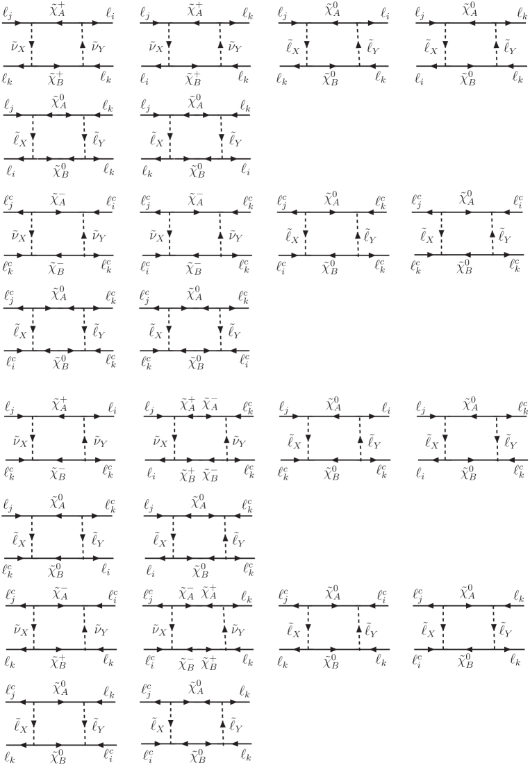
Figure 16: Box diagrams relevant for the computation of the coefficients $B^{LL}_{ji;k}$ (first and second rows), $B^{RR}_{ji;k}$ (third and fourth rows), $B^{LR}_{ji;k}$ (fifth and sixth rows) and $B^{RL}_{ji;k}$ (seventh and eighth rows) [see Eqs. (C-1)-(Appendix C-Box coefficients for the $\bm{\ell_{j}\to\ell_{i}\ell_{k}\ell_{k}\,(i\neq k)}$ amplitudes)].

References

- [1] S. Weinberg, Phys. Rev. Lett. 43 (1979) 1566.
- [2] P. Minkowski, Phys. Lett. B 67 421 (1977); M. Gell-Mann, P. Ramond and R. Slansky, in Supergravity, eds. P. Van Nieuwenhuizen and D. Freedman (North-Holland, Amsterdam, 1979),p. 315; T. Yanagida, in Proceedings of the Workshop on the Unified Theory and the Baryon Number in the Universe, eds. O. Sawada and A. Sugamoto (KEK, Tsukuba, 1979), p. 95; S.L. Glashow, in Quarks and Leptons, eds. M. Lévy et al., (Plenum, 1980, New-York), p. 707; R.N. Mohapatra and G. Senjanović, Phys. Rev. Lett. 44, 912 (1980).
- [3] R. Foot, H. Lew, X. G. He and G. C. Joshi, Z. Phys. C 44 (1989) 441; E. Ma, Phys. Rev. Lett. 81 (1998) 1171;B. Brahmachari, E. Ma and U. Sarkar, Phys. Lett. B 520 (2001) 152.
- [4] R. Barbieri, D.V. Nanopolous, G. Morchio and F. Strocchi, Phys. Lett. B 90, 91 (1980); R. E. Marshak and R. N. Mohapatra, VPI-HEP-80/02 Invited talk given at Orbis Scientiae, Coral Gables, Fla., Jan 14-17, 1980; T. P. Cheng and L. F. Li, Phys. Rev. D 22, 2860 (1980); M. Magg and Ch. Wetterich, Phys. Lett. B 94, 61 (1980); J. Schechter and J. W. F. Valle, Phys. Rev. D 22, 2227 (1980); G. Lazarides, Q. Shafi and C. Wetterich, Nucl. Phys. B 181, 287 (1981); R.N. Mohapatra and G. Senjanovic, Phys. Rev. D 23, 165 (1981); E. Ma and U. Sarkar, Phys. Rev. Lett. 80, 5716 (1998).
- [5] J. A. Casas, V. Di Clemente, A. Ibarra and M. Quiros, Phys. Rev. D 62 (2000) 053005.
- [6] J. R. Ellis and D. V. Nanopoulos, Phys. Lett. B 110, 44 (1982); R. Barbieri and R. Gatto, Phys. Lett. B 110, 211 (1982); M. J. Duncan, Nucl. Phys. B 221, 285 (1983); J. F. Donoghue, H. P. Nilles and D. Wyler, Phys. Lett. B 128, 55 (1983).
- [7] F. Borzumati and A. Masiero, Phys. Rev. Lett. 57, 961 (1986).
- [8] F. Gabbiani and A. Masiero, Nucl. Phys. B 322, 235 (1989).
- [9] A. Rossi, Phys. Rev. D 66, 075003 (2002).
- [10] See A. Casas and A. Ibarra in Ref. [12] and S. Davidson and A. Ibarra, JHEP 0109 (2001) 013.
- [11] J. Hisano, T. Moroi, K. Tobe and M. Yamaguchi, Phys. Rev. D 53, 2442 (1996).
- [12] J. Hisano, D. Nomura and T. Yanagida, Phys. Lett. B 437, 351 (1998); J. Hisano and D. Nomura, Phys. Rev. D 59 (1999) 116005; J. R. Ellis, M. E. Gomez, G. K. Leontaris, S. Lola and D. V. Nanopoulos, Eur. Phys. J. C 14 (2000) 319; J. A. Casas and A. Ibarra, Nucl. Phys. B 618, 171 (2001); D. F. Carvalho, J. R. Ellis, M. E. Gomez and S. Lola, Phys. Lett. B 515 (2001) 323; S. Lavignac, I. Masina and C. A. Savoy, Phys. Lett. B 520, 269 (2001); A. Kageyama, S. Kaneko, N. Shimoyama and M. Tanimoto, Phys. Rev. D 65 (2002) 096010; A. Masiero, S. K. Vempati and O. Vives, Nucl. Phys. B 649, 189 (2003); K. S. Babu, B. Dutta and R. N. Mohapatra, Phys. Rev. D 67 (2003) 076006;T. Blazek and S. F. King, Nucl. Phys. B 662 (2003) 359; S. T. Petcov, S. Profumo, Y. Takanishi and C. E. Yaguna, Nucl. Phys. B 676 (2004) 453; M. Hirsch, J. C. Romao, S. Skadhauge, J. W. F. Valle and A. Villanova del Moral, Phys. Rev. D 69 (2004) 093006; E. Arganda and M. J. Herrero, Phys. Rev. D 73, 055003 (2006); L. Calibbi, A. Faccia, A. Masiero and S. K. Vempati, arXiv:hep-ph/0605139; P. Hosteins, S. Lavignac and C. A. Savoy, arXiv:hep-ph/0606078; S. Antusch, E. Arganda, M. J. Herrero and A. M. Teixeira, arXiv:hep-ph/0607263.
- [13] F. R. Joaquim and A. Rossi, Phys. Rev. Lett. 97 (2006) 181801.
- [14] T. Hambye, E. Ma and U. Sarkar, Nucl. Phys. B 602 (2001) 23.
- [15] S. Eidelman et al. [Particle Data Group], Phys. Lett. B 592 (2004) 1.
- [16] L. J. Hall and L. Randall, Phys. Rev. Lett. 65 (1990) 2939.
- [17] V. Cirigliano, B. Grinstein, G. Isidori and M. B. Wise, Nucl. Phys. B 728 (2005) 121; B. Grinstein, V. Cirigliano, G. Isidori and M. B. Wise, arXiv:hep-ph/0608123; S. Davidson and F. Palorini, arXiv:hep-ph/0607329; G. C. Branco, A. J. Buras, S. Jager, S. Uhlig and A. Weiler, arXiv:hep-ph/0609067.
- [18] V. S. Kaplunovsky and J. Louis, Phys. Lett. B 306 (1993) 269; A. Brignole, L. E. Ibanez and C. Munoz, Nucl. Phys. B 422 (1994) 125 [Erratum-ibid. B 436 (1995) 747].
- [19] L. J. Hall, V. A. Kostelecky and S. Raby, Nucl. Phys. B 267 (1986) 415.
- [20] R. Barbieri and L. J. Hall, Phys. Lett. B 338 (1994) 212.
- [21] E. J. Chun, A. Masiero, A. Rossi and S. K. Vempati, Phys. Lett. B 622, 112 (2005).
- [22] C. Bachas, C. Fabre and T. Yanagida, Phys. Lett. B 370, 49 (1996); S. Chaudhuri, G. Hockney and J. D. Lykken, Nucl. Phys. B 469, 357 (1996); T. Han, T. Yanagida and R. J. Zhang, Phys. Rev. D 58, 095011 (1998); B. Brahmachari, Phys. Rev. D 65, 067502 (2002); I. Dorsner and P. F. Perez, Nucl. Phys. B 723, 53 (2005); I. Dorsner, P. F. Perez and R. Gonzalez Felipe, Nucl. Phys. B 747, 312 (2006).
- [23] P. Langacker and B. D. Nelson, Phys. Rev. D 72 (2005) 053013 [arXiv:hep-ph/0507063].
- [24] M. Cvetic, I. Papadimitriou and G. Shiu, Nucl. Phys. B 659 (2003) 193 [Erratum-ibid. B 696 (2004) 298]; M. Cvetic and P. Langacker, arXiv:hep-th/0607238.
- [25] H. Georgi and C. Jarlskog, Phys. Lett. B 86, 297 (1979); J. A. Harvey, P. Ramond and D. B. Reiss, Phys. Lett. B 92, 309 (1980); For more recent works see for example: K. S. Babu and S. M. Barr, Phys. Rev. D 56, 2614 (1997); Z. Berezhiani, Phys. Lett. B 417, 287 (1998); R. Barbieri, L. J. Hall, S. Raby and A. Romanino, Nucl. Phys. B 493, 3 (1997); Z. Berezhiani and A. Rossi, JHEP 9903, 002 (1999); Z. Berezhiani and A. Rossi, Nucl. Phys. B 594, 113 (2001); G. Altarelli, F. Feruglio and I. Masina, JHEP 0011 (2000) 040.
- [26] S. Dimopoulos and H. Georgi, Nucl. Phys. B 193 (1981) 150; N. Sakai, Z. Phys. C 11, 153 (1981); E. Witten, Nucl. Phys. B 188, 513 (1981).
- [27] M. Dine, W. Fischler and M. Srednicki, Nucl. Phys. B 189, 575 (1981); S. Dimopoulos and S. Raby, Nucl. Phys. B 192, 353 (1981); L. Alvarez-Gaume, M. Claudson and M. B. Wise, Nucl. Phys. B 207, 96 (1982); C. R. Nappi and B. A. Ovrut, Phys. Lett. B 113, 175 (1982); S. Dimopoulos and S. Raby, Nucl. Phys. B 219, 479 (1983); M. Dine and A. E. Nelson, Phys. Rev. D 48, 1277 (1993); M. Dine, A. E. Nelson and Y. Shirman, Phys. Rev. D 51, 1362 (1995).
- [28] For a recent review see G. F. Giudice and R. Rattazzi, Phys. Rept. 322, 419 (1999).
- [29] M. Dine, Y. Nir and Y. Shirman, Phys. Rev. D 55 (1997) 1501 [arXiv:hep-ph/9607397].
- [30] L. V. Avdeev, D. I. Kazakov and I. N. Kondrashuk, Nucl. Phys. B 510 (1998) 289; G. F. Giudice and R. Rattazzi, Nucl. Phys. B 511, 25 (1998); N. Arkani-Hamed, G. F. Giudice, M. A. Luty and R. Rattazzi, Phys. Rev. D 58, 115005 (1998); C. E. M. Wagner, Nucl. Phys. B 528, 3 (1998).
- [31] Z. Chacko and E. Ponton, Phys. Rev. D 66 (2002) 095004.
- [32] For a string-inspired realization of GMSB see e.g. E. Floratos and C. Kokorelis, arXiv:hep-th/0607217.
- [33] G. R. Dvali and M. A. Shifman, Phys. Lett. B 399 (1997) 60; Z. Chacko, E. Katz and E. Perazzi, Phys. Rev. D 66 (2002) 095012.
- [34] See e.g. , M. C. Gonzalez-Garcia, Phys. Scripta T121 (2005) 72; G. L. Fogli, E. Lisi, A. Marrone and A. Palazzo, Prog. Part. Nucl. Phys. 57, 742 (2006); A. Strumia and F. Vissani, Nucl. Phys. B 726, 294 (2005); R. N. Mohapatra and A. Y. Smirnov, arXiv:hep-ph/0603118; J. W. F. Valle, arXiv:hep-ph/0603223.
- [35] M. L. Brooks et al. [MEGA Collaboration], Phys. Rev. Lett. 83, 1521 (1999).
- [36] M. Grassi [MEG Collaboration], Nucl. Phys. Proc. Suppl. 149 (2005) 369.
- [37] B. Aubert et al. [BABAR Collaboration], Phys. Rev. Lett. 95, 041802 (2005).
- [38] A. G. Akeroyd et al. [SuperKEKB Physics Working Group], arXiv:hep-ex/0406071.
- [39] B. Aubert et al. [BABAR Collaboration], Phys. Rev. Lett. 96, 041801 (2006).
- [40] U. Bellgardt et al. [SINDRUM Collaboration], Nucl. Phys. B 299 (1988) 1.
- [41] J. Aysto et al., arXiv:hep-ph/0109217; B. L. Roberts, M. Grassi and A. Sato, Nucl. Phys. Proc. Suppl. 155 (2006) 123.
- [42] B. Aubert et al. [BABAR Collaboration], arXiv:hep-ex/0312027.
- [43] Y. Yusa, H. Hayashii, T. Nagamine and A. Yamaguchi [Belle Collaboration], eConf C0209101 (2002) TU13 [Nucl. Phys. Proc. Suppl. 123 (2003) 95] [arXiv:hep-ex/0211017].
- [44] M. Hodgkinson [BaBar Collaboration], Nucl. Phys. Proc. Suppl. 144 (2005) 167.
- [45] J. Kaulard et al. [SINDRUM II Collaboration], Phys. Lett. B 422 (1998) 334.
- [46] Y. Mori et al. [PRISM/PRIME Working group], LOI at J-PARC 50-GeV PS, LOI-25 [http:// psux1.kek.jp/jhf-np/LOIlist/LOIlist.html].
- [47] R. Barate et al. [LEP Working Group for Higgs boson searches], Phys. Lett. B 565 (2003) 61.
- [48] S. Heinemeyer, W. Hollik and G. Weiglein, Comput. Phys. Commun. 124, 76 (2000).
- [49] See for a review see e.g., M. Passera, Nucl. Phys. Proc. Suppl. 155 (2006) 365.
- [50] [Tevatron Electroweak Working Group], arXiv:hep-ex/0603039.
- [51] See e.g., N. K. Falck, Z. Phys. C 30, 247 (1986); S. P. Martin and M. T. Vaughn, Phys. Rev. D 50, 2282 (1994).
- [52] For studies on the sparticle spectrum in GMSB models see e.g., S. Dimopoulos, S. D. Thomas and J. D. Wells, Nucl. Phys. B 488, 39 (1997); A. Strumia, Phys. Lett. B 409, 213 (1997).
- [53] D. M. Pierce, J. A. Bagger, K. T. Matchev and R. j. Zhang, Nucl. Phys. B 491 (1997) 3.
- [54] For a review see N. V. Krasnikov and V. A. Matveev, Phys. Usp. 47, 643 (2004) [Usp. Fiz. Nauk 174, 697 (2004)] and http://CMSinfo.cern.ch/Welcome.html/CMSdocuments/CMSplots.
- [55] M. Carena and H. E. Haber, Prog. Part. Nucl. Phys. 50 (2003) 63, and references therein.
- [56] A. Brignole and A. Rossi, Nucl. Phys. B 701, 3 (2004).
- [57] K. S. Babu and C. Kolda, Phys. Rev. Lett. 89 (2002) 241802;A. Dedes, J. R. Ellis and M. Raidal, Phys. Lett. B 549 (2002) 159.
- [58] A. Brignole and A. Rossi, Phys. Lett. B 566 (2003) 217.
- [59] See E. Arganda and M. J. Herrero in [12].
- [60] F. Gabbiani, E. Gabrielli, A. Masiero and L. Silvestrini, Nucl. Phys. B 477 (1996) 321; J. Foster, K. i. Okumura and L. Roszkowski, JHEP 0603 (2006) 044.
- [61] M. A. Giorgi et al. [SuperB group], INFN Roadmap Report, March 2006.
- [62] M. Komatsu, P. Migliozzi and F. Terranova, J. Phys. G 29, 443 (2003); P. Migliozzi and F. Terranova, Phys. Lett. B 563, 73 (2003); P. Huber, J. Kopp, M. Lindner, M. Rolinec and W. Winter, JHEP 0605, 072 (2006).
- [63] For a recent rewiew, see A. Blondel, A. Cervera-Villanueva, A. Donini, P. Huber, M. Mezzetto and P. Strolin, arXiv:hep-ph/0606111.
- [64] M. Fukugita and T. Yanagida, Phys. Lett. B 174 (1986) 45.
- [65] G. C. Branco, R. Gonzalez Felipe, F. R. Joaquim and M. N. Rebelo, Nucl. Phys. B 640 (2002) 202; W. Buchmuller, P. Di Bari and M. Plumacher, Nucl. Phys. B 643 (2002) 367; G. C. Branco, R. Gonzalez Felipe, F. R. Joaquim, I. Masina, M. N. Rebelo and C. A. Savoy, Phys. Rev. D 67 (2003) 073025; S. Pascoli, S. T. Petcov and W. Rodejohann, Phys. Rev. D 68 (2003) 093007; E. K. Akhmedov, M. Frigerio and A. Y. Smirnov, JHEP 0309 (2003) 021; G. F. Giudice, A. Notari, M. Raidal, A. Riotto and A. Strumia, Nucl. Phys. B 685 (2004) 89; T. Hambye, Y. Lin, A. Notari, M. Papucci and A. Strumia, Nucl. Phys. B 695 (2004) 169; R. Gonzalez Felipe, F. R. Joaquim and B. M. Nobre, Phys. Rev. D 70 (2004) 085009; W. Buchmuller, P. Di Bari and M. Plumacher, Annals Phys. 315 (2005) 305; G. C. Branco, R. Gonzalez Felipe, F. R. Joaquim and B. M. Nobre, Phys. Lett. B 633 (2006) 336; A. Abada, S. Davidson, F. X. Josse-Michaux, M. Losada and A. Riotto, JCAP 0604 (2006) 004; E. Nardi, Y. Nir, E. Roulet and J. Racker, JHEP 0601 (2006) 164; A. Abada, S. Davidson, A. Ibarra, F. X. Josse-Michaux, M. Losada and A. Riotto, arXiv:hep-ph/0605281; V. Cirigliano, G. Isidori and V. Porretti, arXiv:hep-ph/0607068; K. Bhattacharya, N. Sahu, U. Sarkar and S. K. Singh, arXiv:hep-ph/0607272.
- [66] G. D’Ambrosio, T. Hambye, A. Hektor, M. Raidal and A. Rossi, Phys. Lett. B 604, 199 (2004); For previous works on resonant leptogenesis in different contexts see e.g., M. Flanz, E. A. Paschos and U. Sarkar, Phys. Lett. B 345 (1995) 248 [Erratum-ibid. B 382 (1996) 447]; L. Covi, E. Roulet and F. Vissani, Phys. Lett. B 384 (1996) 169; M. Flanz, E. A. Paschos, U. Sarkar and J. Weiss, Phys. Lett. B 389 (1996) 693; G. D’Ambrosio, G. F. Giudice and M. Raidal, Phys. Lett. B 575 (2003) 75; Y. Grossman, T. Kashti, Y. Nir and E. Roulet, Phys. Rev. Lett. 91 (2003) 251801; Nucl. Phys. B 692 (2004) 303.
- [67] T. Hambye and G. Senjanovic, Phys. Lett. B 582 (2004) 73; S. Antusch and S. F. King, Phys. Lett. B 597 (2004) 199; T. Hambye, arXiv:hep-ph/0412053; T. Hambye, M. Raidal and A. Strumia, Phys. Lett. B 632 (2006) 667.
- [68] Y. Farzan, JHEP 0502 (2005) 025.