Neutrino reconstruction with topological information

Abstract

In general a decay with a missing (not detected) particle can not be fully reconstructed apart from a few exceptions. For example, if the momentum of the decaying particle is known or if the missing energy in an event is measured precisely, then the missing particle 4-momentum can be determined. Here a new method is proposed that utilizes additional information about the topology of a decay: The direction from the primary to the secondary vertex combined with momentum conservation allows the determination of the missing particle momentum up to a twofold ambiguity. The semileptonic decay of the $B^{0}_{s}$ mesons is considered as an example to illustrate this method and to compare its performance against conventional approaches.

, , ,

1 Introduction

Generally it is considered that the decay of a particle, where one of the final state products is not detected, can not be fully reconstructed. There are a few well known exceptions. If the momentum of the decaying particle is known and all but one of the decay products are detected and reconstructed then, obviously, it is possible to determine the missing particle’s 4-momentum. Another possibility to measure the momentum of missing particle is based on the hermeticity of the detector where the missing energy is measured sufficiently well. An approximate method is used in studies of $B^{0}_{s}{\kern-1.60004pt\kern 1.79993pt\overline{\kern-1.79993ptB}{}^{0}_{s}}$ oscillations with semileptonic decays where the neutrino is a missing particle. The reconstruction of the $B^{0}_{s}$ meson momentum is a key ingredient in these studies. For this purpose, a $k$-factor is introduced which is the ratio between the momentum of the measured decay products and the original $B^{0}_{s}$ momentum. The $k$-factor is obtained from Monte Carlo (MC) studies. The use of the $k$-factor induces a large error on the proper time of the $B^{0}_{s}$.

In this paper we point out that by including additional topological information the neutrino 4-momentum can be reconstructed up to a twofold ambiguity. The study of $B^{0}_{s}{\kern-1.60004pt\kern 1.79993pt\overline{\kern-1.79993ptB}{}^{0}_{s}}$- oscillations in the semileptonic decay of the $B^{0}_{s}$ meson at hadron colliders is used to illustrate the method of the neutrino 4-momentum reconstruction.

2 Kinematics of the Semileptonic $B^{0}_{s}$ Decay

Consider the decay $B^{0}_{s}\rightarrow D^{-}_{s}\ell^{+}\nu$ where the $D^{-}_{s}$ meson decays into a final state with charged hadrons and all hadrons are reconstructed. The kinematics of such a decay can be described by four equations in three dimensions:

$$\sqrt{m_{B}^{2}+\vec{P}_{B}^{2}}=\sqrt{m_{(D_{s}\ell)}^{2}+\vec{P}_{(D_{s}\ell)}^{2}}+|\vec{P}_{\nu}|$$ (1)

$$\vec{P}_{B}=\vec{P}_{(D_{s}\ell)}+\vec{P}_{\nu}$$ (2)

In this system of equations there are six unknown variables: $P_{B}^{i}$, $P_{\nu}^{i}$, where $i$ stands for $x$, $y$ and $z$. Since there are only four equations, the system is undetermined.

The flight direction of the $B^{0}_{s}$ meson, $\vec{V}_{B}$, obtained from the primary and secondary vertex, provides the necessary information to solve for the neutrino momentum. Without loss of generality one can work in a two dimensional coordinate system: one axis ($\parallel$) is defined by the $B^{0}_{s}$ flight direction $\vec{V}_{B}$, the other one ($\perp$) is defined in the plane spanned by the two vectors $\vec{P}_{D_{s}\ell}$ and $\vec{V}_{B}$ and is orthogonal to the $B^{0}_{s}$ flight direction. $\Theta$ is the angle between the flight directions of the $B^{0}_{s}$ meson and the $D_{s}\ell$ system. Then one gets:

$$\sqrt{m_{B}^{2}+\vec{P}_{B}^{2}} = \sqrt{m_{(D_{s}\ell)}^{2}+\vec{P}_{(D_{s}\ell)}^{2}}+|\vec{P}_{\nu}|$$ (3)

$$|\vec{P}_{B}| = P_{(D_{s}\ell)}^{\parallel}+P_{\nu}^{\parallel}$$ (4)

$$\vec{P}_{\nu}^{2} = (P_{\nu}^{\parallel})^{2}+(P_{\nu}^{\perp})^{2}$$ (5)

$$\vec{P}_{(D_{s}\ell)}^{2} = (P_{(D_{s}\ell)}^{\parallel})^{2}+(P_{(D_{s}\ell)}^{\perp})^{2}$$ (6)

$$P_{(D_{s}\ell)}^{\parallel} = |\vec{P}_{(D_{s}\ell)}|\times\cos{\Theta}$$ (7)

$$\cos{\Theta} = \frac{\vec{P}_{(D_{s}\ell)}\cdot\vec{V}_{B}}{|\vec{P}_{(D_{s}\ell)}||\vec{V}_{B}|}$$ (8)

The momentum components of the $D_{s}\ell$ system and of the neutrino orthogonal to the $B^{0}_{s}$ flight direction are of equal magnitude and opposite sign:

$$P_{(D_{s}\ell)}^{\perp} = -P_{\nu}^{\perp}$$ (9)

Therefore the neutrino momentum component along the $B^{0}_{s}$ flight direction can be obtained with a straightforward calculation:

$$P_{\nu}^{\parallel} = -a\pm\sqrt{r}$$ (10)

where

$$a = \frac{(m_{B}^{2}-m_{(D_{s}\ell)}^{2}-2\cdot(P_{(D_{s}\ell)}^{\perp})^{2})\cdot P_{(D_{s}\ell)}^{\parallel}}{2\cdot((P_{(D_{s}\ell)}^{\parallel})^{2}-E_{(D_{s}\ell)}^{2})}$$ (11)

$$r = \frac{(m_{B}^{2}-m_{(D_{s}\ell)}^{2}-2\cdot(P_{(D_{s}\ell)}^{\perp})^{2})^{2}\cdot E_{(D_{s}\ell)}^{2}}{4\cdot((P_{(D_{s}\ell)}^{\parallel})^{2}-E_{(D_{s}\ell)}^{2})^{2}}+\frac{E_{(D_{s}\ell)}^{2}\cdot(P_{(D_{s}\ell)}^{\perp})^{2}}{(P_{(D_{s}\ell)}^{\parallel})^{2}-E_{(D_{s}\ell)}^{2}}$$ (12)

Eq. 10 leads to two solutions, only one of them is correct. In an experimental environment there might be no solution of this equation if the radicand $r$ is negative due to finite vertex and momentum resolutions. In the following we illustrate that despite these facts the method still provides competitive results with respect to conventional approaches.

3 MC simulations

To verify that the proposed method works not only in ideal conditions without experimental errors, a MC simulation has been developed to study $B^{0}_{s}{\kern-1.60004pt\kern 1.79993pt\overline{\kern-1.79993ptB}{}^{0}_{s}}$ - mixing in the semileptonic decay mode. The PYTHIA V6.227 [1] package has been used as an event generator with a center-of-mass energy of 14 TeV. We have generated 45000 events each containing two b quarks. One of them hadronizes to a $B^{0}_{s}$ meson and decays according to

$$B^{0}_{s}\ \rightarrow D_{s}\mu^{+}\nu_{\mu},\qquad D_{s}\rightarrow\phi\pi^{-},\qquad\phi\rightarrow K^{+}K^{-};$$ (13)

the second $b$ quark hadronizes according to PYTHIA into a $b$-hadron and decays unconstrained. The decay in (13) is called ‘signal’ decay to distinguish it from the other $b$-hadron decay.

All hadrons from the signal decay are required to have $\mbox{$p_{T}$}\geq 1{\mathrm{\,Ge\kern-1.00006ptV\!/}c}$, the muon is required to have $p_{T}\geq 3{\mathrm{\,Ge\kern-1.00006ptV\!/}c}$. The track parameters and vertex positions (primary and secondary) have been smeared according to Gaussian distributions with the following parameters. The momentum uncertainty has been simulated by smearing the pseudorapidity with $\sigma_{\eta}=5.8\times 10^{-4}$, the angle $\phi$ with $\sigma_{\phi}=0.58\rm\,mrad$ and the inverse transverse momentum with $\sigma_{(1/p_{T})}=0.013(GeV/c)^{-1}$. The primary vertex has been smeared with $\sigma_{x,y}=20\,\mu\rm m$ in both, x- and y-direction, the secondary vertex has been smeared with $\sigma_{||}=70\,\mu\rm m$ in flight direction of the $B^{0}_{s}$ and $\sigma_{\perp}=10\,\mu\rm m$ in the perpendicular direction.

4 Proper time reconstruction

The most important ingredient in the measurement of the $B^{0}_{s}$ oscillation frequency is the proper time calculated in the transverse plane as follows:

$$c\tau=\frac{L_{xy}\,m(B^{0}_{s})}{p_{T}(B^{0}_{s})},$$ (14)

where $L_{xy}$ is the flight path length, $m(B^{0}_{s})$ and $p_{T}(B^{0}_{s})$ are the mass and transverse momentum of the $B^{0}_{s}$ meson respectively.

In the semileptonic $B^{0}_{s}$ meson decay, the neutrino is not detected and the $p_{T}$ of the $B^{0}_{s}$ meson cannot be measured directly. Therefore a correction factor, derived from MC simulations, is introduced to scale the measured transverse momentum of the $D_{s}\ell$ system. Eq. 14 is modified as follows

$$c\tau=\frac{L_{xy}\,m(B^{0}_{s})}{p_{T}(D_{s}\ell)}\times k,$$ (15)

with the $k$-factor estimated from MC simulations and calculated as

$$k=\frac{p_{T}(D_{s}\ell)}{p_{T}(B^{0}_{s})}.$$ (16)

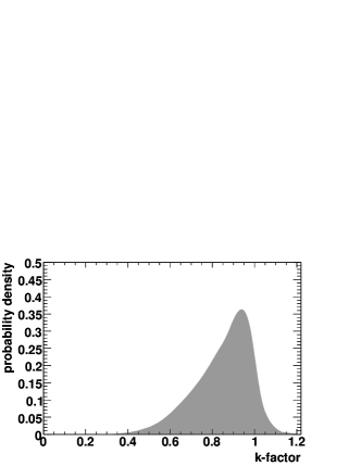
Figure 1: Probability density for the $k$-factor.

This $k$-factor (see Fig. 1) introduces a significant error on the $B^{0}_{s}$ momentum and, hence, on the proper time as well. To reduce the error by an average $k$-factor, it is calculated in bins of $m_{(D_{s}\ell)}$. We illustrate in Fig. 2 the $B^{0}_{s}$  meson transverse momentum resolution as a function of the invariant mass of the $D_{s}\ell$ system for the $k$-factor and the neutrino reconstruction method. It is evident that the resolution obtained with the neutrino reconstruction method is substantially better than with the $k$-factor method. Note that the neutrino reconstruction method is sensitive to $\sigma_{\perp}$, therefore two different performances for $\sigma_{\perp}=10\,\mu\rm m$ and $\sigma_{\perp}=30\,\mu\rm m$ are shown.

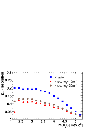
Figure 2: $B^{0}_{s}$ momentum resolution calculated with $k$-factor and neutrino reconstruction methods.

Fig. 3 illustrates the proper time resolution obtained with the $k$-factor method (a) and the neutrino reconstruction method (b). For the latter method the closest to the true value solutions are filled in the histogram. The distributions are fitted with two Gaussian, the average width $\sigma$ is determined according to

$$\sigma^{2}=\frac{N_{n}^{2}\sigma_{n}^{2}+N_{w}^{2}\sigma_{w}^{2}}{N_{n}^{2}+N_{w}^{2}},$$ (17)

where $\sigma_{n}$ ($\sigma_{w}$) and $N_{n}$ ($N_{w}$) are the width and normalization of the narrow (wide) Gaussian, respectively. For the $k$-factor method $\sigma_{n}=100\rm\,fs$ ($\sigma_{w}=338\rm\,fs$) and $N_{n}=2700$ ($N_{w}=730$) that gives an average $\sigma=132\rm\,fs$. For the neutrino reconstruction method $\sigma_{n}=77\rm\,fs$ ($\sigma_{w}=193\rm\,fs$) and $N_{n}=2300$ ($N_{w}=660$) that gives an average $\sigma=91\rm\,fs$. The neutrino reconstruction method provides a proper time resolution which is better than in the reconstruction done with the $k$-factor method.

Figure 3: Proper time resolution. (a) $k$-factor method, (b) neutrino reconstruction method.

5 Amplitude Fit

A standard way to search for $B^{0}_{s}$ oscillations is the amplitude method described in Ref. [2]. Briefly it consists of the following steps. Candidates for the decay (13) are split into two samples. Events with the same flavor at production and decay time comprise the unmixed sample, events with the opposite flavor constitute the mixed sample. The two cases are distinguished by tagging the flavor of the $B^{0}_{s}$ meson at the production and the decay. Tagging at the production can be achieved by identifying the flavor of the second $b$-hadron in the event; tagging at the decay can be accomplished by identifying the charge of the $B^{0}_{s}$ meson decay products.

In each event, the proper decay time of the $B^{0}_{s}$ mesons is reconstructed and the two event samples are used to define the time-dependent asymmetry

$$a(t)=\frac{P_{unmix}-P_{mix}}{P_{unmix}+P_{mix}}\propto A\times D\times\cos(\Delta m_{s}t),$$ (18)

where $D$ is a global dilution factor accounting for background, miss-tagging and proper-time resolution and $A$ is the amplitude. $P_{unmix}$ and $P_{mix}$ are the time-dependent probability distribution functions for mixed and unmixed $B^{0}_{s}$ meson decays, respectively.

In the fit to the asymmetry distribution, the oscillation frequency $\Delta m_{s}$ is fixed, leaving the amplitude $A$ as a free parameter. A scan over $\Delta m_{s}$ is performed starting from zero. If the fixed value of $\Delta m_{s}$ is consistent with the true one, the fitted amplitude will be equal to unity, else it is consistent with zero. The error on the amplitude value $A$ is calculated according to the formula

$$\sigma_{A}=\frac{1}{1-2W}\times\sqrt{\frac{2}{S+B}}\times\frac{S+B}{S}\times e^{\textstyle\frac{\Delta m_{s}^{2}\sigma_{t}^{2}}{2}},$$ (19)

where $W$ is the mistagging probability, $S$ the number of signal, $B$ the number of background events, and $\sigma_{t}$ the proper time resolution. The amplitude method is sensitive to the tested value of $\Delta m_{s}$ if $\sigma_{A}$ is small compared to unity. The value of $\Delta m_{s}$ at which $1=1.645\times\sigma_{A}$ is quoted as sensitivity limit.

In the following we assume a mistagging probability of $40\%$, a number of 45000 signal events for semileptonic $B^{0}_{s}$ decays and a signal to background ratio of 1:1. The simulated oscillation frequency is taken as $\Delta m_{s}=17.25~{}\mathrm{ps^{-1}}$ [3, 4].

The result of the amplitude fit for the $k$-factor method with the sensitivity curve is presented in Fig. 4a. The sensitivity of the method for the processed number of signal events is about 17 $\mathrm{ps^{-1}}$.

On Fig. 4b one can see the result of the amplitude fit done on the events reconstructed with the neutrino reconstruction method. The sensitivity to $\Delta m_{s}$ is about 21 $\mathrm{ps^{-1}}$. In this case there is a clear peak in the amplitude fit at the input value of $\Delta m_{s}=17.25~{}\mathrm{ps^{-1}}$.

Figure 4: Amplitude fits for $B^{0}_{s}{\kern-1.60004pt\kern 1.79993pt\overline{\kern-1.79993ptB}{}^{0}_{s}}$ oscillations. (a) $k$-factor method, (b) neutrino reconstruction method.

6 Discussion

On the one hand the use of the neutrino reconstruction method improves the momentum resolution of the $B^{0}_{s}$ meson. On the other hand it degrades the signal to background ratio and reduces the signal sample. First, since solving the system of equations, we end up with a quadratic equation with two solutions. One solution is the ‘true’, the other is the ‘wrong’ one. In such a way the number of background events is increased by the number of wrong solutions from the signal as well as from the background sample. Second, again due to the quadratic equation and the realistic resolutions, a certain fraction of events has a negative radicand $r$ and, hence, there is no solution for the $B^{0}_{s}$ meson momentum. These events are excluded from the analysis (both from signal and background samples).

With the resolutions used in this analysis the number of signal events is decreased by a factor of 2 roughly (the same is true also for background) and the number of background events is increased by a factor of 3 (due to the ‘wrong’ signal and background events). Hence, in the neutrino reconstruction method the signal to background ratio is not 1:1 (like in the $k$-factor method) but 1:3. Despite these facts the sensitivity of the neutrino reconstruction method is still at higher values of $\Delta m_{s}$ compared to the $k$-factor method.

Also the quality of both methods with respect to the primary (Fig. 5a) and secondary (Fig. 5b) vertex resolution is investigated, when all other resolutions are kept constant. From these figures one can conclude that the neutrino reconstruction method is more powerful than the $k$-factor method if $\sigma_{\perp}\lesssim 45\mu$m and $\sigma_{x,y}\lesssim 45\mu$m. For a typical hadron collider detector resolutions better than quoted above are achievable [5, 6, 7, 8].

Figure 5: Sensitivity as a function of (a) the primary vertex resolution $\sigma_{x,y}$ and (b) the secondary vertex resolution $\sigma_{\perp}$ for neutrino reconstruction and $k$-factor methods.

7 Conclusion

In this paper we have shown that the full neutrino reconstruction is possible in decays like the semileptonic $B^{0}_{s}$ decay mode where all but one final state particle are measured. For this one has to use additional topological information, in our example the direction of the $B^{0}_{s}$ meson momentum. The search for the $B^{0}_{s}{\kern-1.60004pt\kern 1.79993pt\overline{\kern-1.79993ptB}{}^{0}_{s}}$ oscillations has been used as an illustration of the method. For the verification of our procedure we have used typical resolutions of hadron collider detectors. The sensitivity obtained with the neutrino reconstruction method is much higher than with the convenient method used for this decay mode.

Finally, we would like to stress that the proposed method can be used not only in semileptonic $B$ decays but in some other cases where the known topology of a decay can compensate for the incompleteness of kinematical information.

8 Acknowledgment

We would like to thank our colleagues from PSI for fruitful discussions. This research was supported by the Swiss National Science Foundation (SNF).

References

- [1] T. Sjostrand, S. Mrenna and P. Skands, “PYTHIA 6.4 physics and manual,” JHEP 0605 (2006) 026 [arXiv:hep-ph/0603175].
- [2] H. G. Moser and A. Roussarie, “Mathematical methods for oscillation analyses,” Nucl. Instrum. Meth. A 384 (1997) 491.
- [3] A. Abulencia [CDF - Run II Collaboration], “Measurement of the oscillation frequency,” arXiv:hep-ex/0606027.
- [4] V. M. Abazov et al. [D0 Collaboration], “First direct two-sided bound on the oscillation frequency,” arXiv:hep-ex/0603029.
- [5] A. Starodumov, Z. Xie, “ decay vertex resolution,” CMS NOTE 1997/85.
- [6] ATLAS Collaboration, “ATLAS: Detector and physics performance technical design report. Volume 1,” CERN-LHCC-99-14.
- [7] F. Abe et al. [CDF Collaboration], “Measurement of the meson lifetime using semileptonic decays,” Phys. Rev. D 59 (1999) 032004 [arXiv:hep-ex/9808003].
- [8] V. M. Abazov et al. [D0 Collaboration], “A precise measurement of the lifetime,” arXiv:hep-ex/0604046.