Abstract

We study the indirect detection of neutralino dark matter using positrons and gamma rays from its annihilation in the galactic halo. Considering the HESS data as the spectrum constituting the gamma–ray background, we compare the prospects for the experiments GLAST and PAMELA in a general supergravity framework with non–universal scalar and gaugino masses. We show that with a boost factor of about 10, PAMELA will be competitive with GLAST for typical NFW cuspy profiles.

1 Introduction

The existence of dark matter in the Universe is generally accepted by the scientific community, though its nature is still unknown. One of the most popular candidates, the lightest neutralino, appears naturally in supersymmetric (SUSY) extensions of the standard model. It has long been thought that dark matter particles could be observed indirectly by detecting the products of their annihilations. Such products include gamma-rays, neutrinos and anti–matter. Actually, many experiments have been performed or are planned in order to detect indirectly (or directly) the presence of such particles in the galactic halo [1]. For example, high–energy positron excess in the cosmic rays provides an opportunity to search for the dark matter signal. These fluxes will be measured with unprecedented accuracy by the present space-based experiment PAMELA (Payload for Antimatter–Matter Exploration and Light–nuclei Astrophysics [2]), and also by future experiments like AMS-02 (Alpha Magnetic Spectrometer [3]), designed to be deployed in the International Space Station around 2009–10. The precision measurements of the cosmic positron spectrum to be provided by PAMELA will be very important to identify signatures of dark matter in our Galaxy.

On the other hand, the gamma–ray data, richer than the cosmic particle data, also give us exciting expectations. The gamma–ray detection experiments have the advantage of being able to search for point sources of annihilation radiation. In particular, the center of our Galaxy, given its dark matter density, is one of the most promising sources of diffuse gamma-rays from dark matter annihilation. In addition to the controversial EGRET data [4], atmospheric Cerenkov telescopes like HESS [5] and MAGIC [6] have observed recently a very bright source in this direction. Actually, HESS was able to measure in detail the gamma–ray spectrum. Although fitting the data with a reasonable SUSY model seems quite difficult, one can use them as the astrophysical background for gamma-ray detection [7]. Scheduled to begin its five years mission in 2007, GLAST (gamma–ray Large Area Space Telescope [8]) will be the most sensitive gamma–ray telescope in the energy range of interest ($1-300$ GeV).

Both space-based experiments, PAMELA and GLAST, will provide us their first results around 2009 (before the LHC data). The aim of this work is to compare the detection prospects of these two experiments in the framework of supergravity (SUGRA) models, taking into account the different astrophysical uncertainties: boost factor and halo density profile. In particular, the effect of clumps in the galactic halo may increase substantially the positron fluxes, and this is parameterised by the so-called boost factor. Likewise, cuspy halo profiles may also give rise to larger gamma–ray fluxes. Let us finally remark that although antiproton fluxes may be in principle as competitive as the positron ones, we prefer to carry out the analysis of antiprotons in detail in a future work [9].

The paper is organized then as follows. In section 2 we will review the neutralino characteristics as a dark matter candidate in SUGRA models. In section 3 we will recall the main features of the positron propagation and detection in the light of the PAMELA experiment. Section 4 will be devoted to gamma–rays detection and GLAST prospects. In Section 5 we will compare in detail these two detection modes. Finally, the conclusions are left for section 6.

2 Neutralino dark matter

For the computation of the positron and gamma–ray fluxes it is crucial to evaluate the neutralino annihilation cross section. Of course, for determining this value the theoretical framework must be established. In particular, we will work in the context of the minimal supersymmetric standard model (MSSM). Let us recall that in this framework there are four neutralinos, $\tilde{\chi}^{0}_{i}~{}(i=1,2,3,4)$, since they are the physical superpositions of the fermionic partners of the neutral electroweak gauge bosons, called bino ($\tilde{B}^{0}$) and wino ($\tilde{W}_{3}^{0}$), and of the fermionic partners of the neutral Higgs bosons, called Higgsinos ($\tilde{H}^{0}_{u}$, $\tilde{H}_{d}^{0}$). Thus one can express the lightest neutralino as

$$\tilde{\chi}^{0}_{1}={Z_{11}}\tilde{B}^{0}+{Z_{12}}\tilde{W}_{3}^{0}+{Z_{13}}\tilde{H}^{0}_{d}+{Z_{14}}\tilde{H}^{0}_{u}\ .$$ (2.1)

It is commonly defined that $\tilde{\chi}^{0}_{1}$ is mostly gaugino-like if $P\equiv|{Z_{11}}|^{2}+|{Z_{12}}|^{2}>0.9$, Higgsino-like if $P<0.1$, and mixed otherwise.

In figure 1 we show the relevant Feynman diagrams contributing to neutralino annihilation. As was remarked e.g. in Refs. [10, 11], the annihilation cross section can be significantly enhanced depending on the SUSY model under consideration. We will concentrate here on the SUGRA scenario, where the soft terms are determined at the unification scale, $M_{GUT}\approx 2\times 10^{16}$ GeV, after SUSY breaking, and radiative electroweak symmetry breaking is imposed.

                                                  

$\propto\frac{m_{\chi}m_{f}}{m_{\tilde{f}}^{2}}Z_{11}^{2}~{}~{}~{}$ $\propto\frac{m_{\chi}^{2}}{m_{A}^{2}}\frac{Z_{11}Z_{13,14}}{m_{W}}m_{f_{d}}\tan\beta(\frac{m_{f_{u}}}{\tan\beta})~{}~{}~{}$ $\propto\frac{m_{f}m_{\chi}}{m_{Z}^{2}}Z_{13,14}^{2}~{}$ $\propto\frac{[-Z_{14}V_{21}^{*}+\sqrt{2}Z_{12}V_{11}^{*}]^{2}(-Z_{13}Z_{31}^{*}+Z_{14}Z_{41}^{*})^{2}}{1+m_{\chi_{i}^{+(0)}}^{2}/m_{\chi}^{2}-m_{W(Z)}^{2}/m_{\chi}^{2}}$

Figure 1: Dominant neutralino annihilation diagrams. Relevant parts of the amplitudes are shown explicitly Terms between parenthesis correspond to $f_{u}$ and $Z$ final states in second and fourth diagrams. V and Z are chargino and neutralino mixing matrices.

2.1 Supergravity models

Let us discuss first the minimal supergravity (mSUGRA) scenario, where the soft terms of the MSSM are assumed to be universal at $M_{GUT}$. Recall that in mSUGRA one has only four free parameters: the soft scalar mass $m$, the soft gaugino mass $M$, the soft trilinear coupling $A$, and the ratio of the Higgs vacuum expectation values, $\tan\beta=\langle H_{u}^{0}\rangle/\langle H_{d}^{0}\rangle$. In addition, the sign of the Higgsino mass parameter, $\mu$, remains also undetermined by the minimization of the Higgs potential.

Since in this scenario the lightest neutralino $\tilde{\chi}^{0}_{1}$ is mainly bino, only ${Z_{11}}$ is large and then the contribution of diagrams in Fig. 1 will be generically small, the first being suppressed by $\tilde{f}$ masses. As a consequence, for example to reproduce in mSUGRA the present experimental accesible regions (EGRET data) is not possible [12] for a typical halo model.

However, as discussed in detail in Ref. [10, 12] in the context of indirect detection, the annihilation cross section can be increased in different ways when the structure of mSUGRA for the soft terms is abandoned. In particular, it is possible to enhance the annihilation channels involving the exchange of the CP-odd Higgs, $A$, by reducing the Higgs mass. In addition, it is also possible to increase the Higgsino components of the lightest neutralino ${Z_{13,14}}$. Thus annihilation channels through Higgs exchange become more important than in mSUGRA. This is also the case for $Z$, $\chi_{1}^{\pm}$, and $\tilde{\chi}_{1}^{0}$-exchange channels. As a consequence, positron and gamma–ray fluxes will be increased.

In particular, the most important effects are produced by the non-universality of Higgs and gaugino masses. These can be parameterised, at $M_{GUT}$, as follows

$$m_{H_{d}}^{2}=m^{2}(1+\delta_{1})\ ,\quad m_{H_{u}}^{2}=m^{2}(1+\delta_{2})\ ,$$ (2.2)

and

$$M_{1}=M\ ,\quad M_{2}=M(1+\delta^{\prime}_{2})\ ,\quad M_{3}=M(1+\delta^{\prime}_{3})\ .$$ (2.3)

We will concentrate in our analysis on the following representative cases:

$$a)\,\,\delta_{1} = 0\ \,\,\,\,\,\,\,\,,\,\,\,\,\delta_{2}\ =\ 0\,\,\,\,\,\,\,\,\,,\,\,\,\,\delta^{\prime}_{2,3}\ =\ 0\ ,$$

$$b)\,\,\delta_{1} = 0\ \,\,\,\,\,\,\,\,,\,\,\,\,\delta_{2}\ =\ 1\ \,\,\,\,\,\,\,\,,\,\,\,\,\delta^{\prime}_{2,3}\ =\ 0\ ,$$

$$c)\,\,\delta_{1} = -1\ \,\,\,\,,\,\,\,\,\delta_{2}\ =\ 0\ \,\,\,\,\,\,\,\,,\,\,\,\,\delta^{\prime}_{2,3}\ =\ 0\ ,$$

$$d)\,\,\delta_{1} = -1\ \,\,\,\,,\,\,\,\,\delta_{2}\ =\ 1\ \,\,\,\,\,\,\,\,,\,\,\,\,\delta^{\prime}_{2,3}\ =\ 0\ \,\,,$$

$$e)\,\,\delta_{1,2} = 0\ \,\,\,\,\,\,\,\,,\,\,\,\,\delta^{\prime}_{2}\ =\ 0\,\,\,\,\,\,\,\,\,,\,\,\,\,\delta^{\prime}_{3}\ =\ -0.5\ ,$$

$$f)\,\,\delta_{1,2} = 0\ \,\,\,\,\,\,\,\,,\,\,\,\,\delta^{\prime}_{2}\ =\ -0.5\,\,\,\,\,\,\,\,\,,\,\,\,\,\delta^{\prime}_{3}\ =\ 0\ .$$ (2.4)

Case a) corresponds to mSUGRA with universal soft terms, cases b), c) and d) correspond to non-universal Higgs masses, and finally cases e) and f) to non-universal gaugino masses. The cases b), c), d), and e) were discussed in Ref. [10], and are known to produce gamma–ray fluxes larger than in mSUGRA, whereas case f) enhances efficiently annihilation processes because of the pure wino nature of the LSP.

Let us remark that for the evaluation of the gamma–ray fluxes and the positron fluxes at production we use the last DarkSusy released version [13]. Concerning the computation of the fluxes observed in the solar neighborhood in the case of adiabatically compressed halos we use our own code. To solve the renormalization group equations (RGEs) for the soft SUSY-breaking terms between $M_{GUT}$ and the electroweak scale, we use the Fortran package SUSPECT [14]. Concerning the positron spectrum observed by PAMELA, we use the annihilation cross section given by DarkSusy at the source, but solve ourselves the propagation equation and calculation of the flux measured on the Earth.

2.2 Experimental and astrophysical constraints

We have taken into account in the computation several experimental and astrophysical bounds. These may produce important constraints on the parameter space of SUGRA models, restricting therefore the regions where the gamma–ray and positron fluxes have to be analyzed.

In particular, concerning the astrophysical constraints, the bounds $0.1\raise 1.29167pt\hbox{$\;<$\kern-7.5pt\raise-4.73611pt\hbox{$\sim\;$}}\Omega_{DM}h^{2}\raise 1.29167pt\hbox{$\;<$\kern-7.5pt\raise-4.73611pt\hbox{$\sim\;$}}0.3$, on the relic neutralino density computation has been considered. Due to its relevance, the WMAP narrow range $0.094\raise 1.29167pt\hbox{$\;<$\kern-7.5pt\raise-4.73611pt\hbox{$\sim\;$}}\Omega_{DM}h^{2}\raise 1.29167pt\hbox{$\;<$\kern-7.5pt\raise-4.73611pt\hbox{$\sim\;$}}0.129$ has also been analyzed in detail.

Concerning the experimental constraints, the lower bounds on the masses of SUSY particles and on the lightest Higgs have been implemented, as well as the experimental bounds on the branching ratio of the $b\to s\gamma$ process and on $a^{\rm SUSY}_{\mu}$. Note that we are using $\mu>0$. We will not consider in the calculation the opposite sign of $\mu$ because this would produce a negative contribution for the $g_{\mu}-2$, and, as will be discussed below, we are mainly interested in positive contributions. Recall that the sign of the contribution is basically given by $\mu M_{2}$, and that $M$, and therefore $M_{2}$, can always be made positive after performing an $U(1)_{R}$ rotation. For $a^{\rm SUSY}_{\mu}$, we have taken into account the recent experimental result for the muon anomalous magnetic moment [15], as well as the most recent theoretical evaluations of the standard model contributions [16]. It is found that when $e^{+}e^{-}$ data are used the experimental excess in $(g_{\mu}-2)$ would constrain a possible SUSY contribution to be $a^{\rm SUSY}_{\mu}=(27.1\pm 10)\times 10^{-10}$. At $2\sigma$ level this implies $7.1\times 10^{-10}\raise 1.29167pt\hbox{$\;<$\kern-7.5pt\raise-4.73611pt\hbox{$\sim\;$}}a^{\rm SUSY}_{\mu}\raise 1.29167pt\hbox{$\;<$\kern-7.5pt\raise-4.73611pt\hbox{$\sim\;$}}47.1\times 10^{-10}$. It is worth noticing here that when tau data are used a smaller discrepancy with the experimental measurement is found. In order not to exclude the latter possibility we will discuss the relevant value $a^{\rm SUSY}_{\mu}=7.1\times 10^{-10}$.

On the other hand, the measurements of $B\to X_{s}\gamma$ decays at CLEO [17] and BELLE [18], lead to bounds on the branching ratio $b\to s\gamma$. In particular we impose on our computation $2.33\times 10^{-4}\leq BR(b\to s\gamma)\leq 4.15\times 10^{-4}$, where the evaluation is carried out using the routine provided by the program micrOMEGAs [19]. This program is also used for our evaluation of $a^{\rm SUSY}_{\mu}$ and relic neutralino density.

3 The positrons in the Galaxy

3.1 The background

The conventional sources of cosmic rays are believed to be supernovae and supernovae remnants, pulsars, compact objects in close binary systems, and stellar winds. Observations of synchrotron emission and $\gamma-$rays reveal the presence of energetic particles in this objects, thus testifying to efficient acceleration processes. Propagation in the interstellar medium changes the initial composition and spectra of cosmic ray species due to the energy losses (ionization, Coulomb scattering, bremsstrahlung, inverse Compton scattering, and synchrotron emission), energy gain (diffusive re-acceleration), and other processes (i.e., diffusion and convection by the galactic wind) [20]. The destruction of primary nuclei via spallation gives rise to secondary nuclei and isotopes which are rare in nature (i.e., Li, Be, B), antiprotons, and pions ($\pi^{\pm},~{}\pi^{0}$) that decay producing secondary $e^{\pm}$ and $\gamma-$rays. The abundance of stable (Li, Be, B, Sc, Ti, V) and radioactive ($Be^{10},~{}Al^{26},~{}Cl^{36},~{}Mn^{54}$) secondaries in cosmic rays are used to derive the diffusion coefficient and the halo size [21]. The result of recent simulations agrees with measurements of the low–energy positron flux in the cosmic rays [21]. The fitting functions for high energy positrons, primary electrons, and secondary electrons have been constructed [22],

$$\Phi_{e^{-}}^{\mathrm{prim}}(E)=\frac{0.16E^{-1.1}}{1+11E^{0.9}+3.2E^{2.15}}~{}\mathrm{(GeV^{-1}cm^{-2}s^{-1}sr^{-1})}\ ,$$ (3.5)

$$\Phi_{e^{-}}^{\mathrm{sec}}(E)=\frac{0.70E^{0.7}}{1+110E^{1.5}+580E^{4.2}}~{}\mathrm{(GeV^{-1}cm^{-2}s^{-1}sr^{-1})}\ ,$$ (3.6)

$$\Phi_{e^{+}}^{\mathrm{sec}}(E)=\frac{4.5E^{0.7}}{1+650E^{2.3}+1500E^{4.2}}~{}\mathrm{(GeV^{-1}cm^{-2}s^{-1}sr^{-1})}\ .$$ (3.7)

3.2 The propagation of a positron

Concerning the propagation of positrons, we will use the "diffusion model" in which the random walk is described by the diffusion equation,

$$\frac{\partial}{\partial t}f(E,r)=K(E)\Delta f(E,r)+\frac{\partial}{\partial E}[b(E)f(E,r)]+Q(E,r)\ ,$$ (3.8)

where $f(E,r)$ denotes the number density of particles per unit of volume and energy and $Q(E,r)$ is the source (positron injection) term generated by neutralino annihilation. The flux of positrons with high energy ($E\gg m_{e}$) around the Sun is given by:

$$\frac{c}{4\pi}f(E,r_{\mathrm{\odot}})\ .$$ (3.9)

Above a few GeV, positron energy losses are dominated by synchrotron radiation in the galactic fields and by inverse Compton scattering on stellar light and on CMB photons. The energy loss rate $b(E)$ depends on the positron energy $E$ through :

$$b(E)=\frac{E^{2}}{E_{0}\tau_{E}}\ ,$$ (3.10)

where we have set the energy reference $E_{0}$ to 1 GeV and the typical energy loss time is $\tau_{E}=10^{16}$ s. We have also assume that the space diffusion coefficient $K(E)$ is written on the form

$$K(E)=K_{0}\left(\frac{E}{E_{0}}\right)^{\alpha}\ ,$$ (3.11)

where the diffusion coefficient at 1 GeV is $K_{0}=3\times 10^{27}\mathrm{cm^{2}s^{-1}}$ with a spectral index of $\alpha=0.6$ [22].

To solve Eq. (3.8) we make the hypothesis that the positron fluxes coming from dark matter annihilation are in equilibrium in the present universe i.e., $\frac{\partial}{\partial t}f(E,r)=0$. Thus Eq. (3.8) simplifies into

$$K_{0}\epsilon^{\alpha}\Delta f(\epsilon,r)+\frac{\partial}{\partial\epsilon}\left[\frac{\epsilon^{2}}{\tau_{E}}f(\epsilon,r)\right]+Q(\epsilon,r)=0\ ,$$ (3.12)

where we have defined $\epsilon=E/E_{0}$.

Concerning the boundary condition, we impose the "free escape" one. This means that the positron density drops to zero on the surface of the diffusion zone. Moreover, we neglect the positrons coming from outside our Galaxy. The diffusion zone (Galaxy) will be parameterised by a cylinder of half height $L=3$ kpc and radius $R=20$ kpc. We will see afterwards that this boundary condition does not affect too much the result around the Sun.

We can see from Eq. (3.8) that the high–energy positrons mainly come from a region within few kpc from the solar system. In fact, this depends mainly on the parameters $K$ and $b$ appearing there. Indeed, positrons far from the Earth lose their energies during the propagation, and consequently they contribute to the low–energy part of the spectrum. Using Eq. (3.8) we can easily approximate the distance in which positrons travel without significant energy loss:

$$r\approx\sqrt{\frac{K(E)E}{b(E)}}=1.8\times(E/1\mathrm{GeV})^{-0.2}~{}~{}\mathrm{kpc}\ ,$$ (3.13)

which gives $r\sim 1.8$ kpc for 1 GeV and $r\sim 0.72$ kpc for a 100 GeV positron. This implies that the influence of the different kinds of dark matter density profiles on the positron fluxes is negligible (recall that all simulations give rise to the same kind of profile around the solar system). Thus the astrophysical dependence of the indirect detection of dark matter through positrons, instead of being similar to the case of the indirect detection through gamma–rays, looks more like the case of the direct detection of dark matter.

To solve Eq. (3.12) we use the treatment given in Ref. [23], where the solution is expressed with the Green function $G$ as :

$$f(\epsilon,r)=\int_{\epsilon_{s}=\epsilon}^{\epsilon_{s}=+\infty}d\epsilon_{s}\int d^{3}r_{s}~{}G(\epsilon,\epsilon_{s},r,r_{s})~{}Q(\epsilon_{s},r_{s})\ ,$$ (3.14)

with

$$G(\epsilon,\epsilon_{s},r,r_{s})=\frac{1-\alpha}{4\pi K_{0}\tau_{E}(\epsilon^{\alpha-1}-\epsilon_{s}^{\alpha-1})}\times\exp\left[\frac{-\rho^{2}(1-\alpha)}{4K_{0}\tau_{E}(\epsilon^{\alpha-1}-\epsilon_{s}^{\alpha-1})}\right]\times V(\epsilon,\epsilon_{s},z,z_{s})\ ,$$ (3.15)

and

$$r=\left[x^{2}+y^{2}+z^{2}\right]^{1/2}~{}~{}~{}~{}~{}\ ,~{}~{}~{}~{}\rho=\left[(x-x_{s})^{2}+(y-y_{s})^{2}\right]^{1/2}.$$ (3.16)

The expression for $V(\epsilon,\epsilon_{s},z,z_{s})$ is obtained using the original method of "electrical images" firstly introduced by Blatz and Edsjo [22]

$$V(\epsilon,\epsilon_{s},z,z_{s}) = \sum_{n=1}^{+\infty}\frac{1}{L}\{\exp\left[-\frac{\lambda_{n}\tau_{E}(\epsilon^{\alpha-1}-\epsilon_{s}^{\alpha-1})}{1-\alpha}\right]\phi_{n}(z_{s})\phi_{n}(z)$$ (3.17)

$$+\exp\left[-\frac{\lambda^{\prime}_{n}\tau_{E}(\epsilon^{\alpha-1}-\epsilon_{s}^{\alpha-1})}{1-\alpha}\right]\phi^{\prime}_{n}(z_{s})\phi^{\prime}_{n}(z)\}\ ,$$

where $\lambda_{n}=K_{0}\times(n-1/2)\frac{\pi}{L}$, $\lambda^{\prime}_{n}=K_{0}\times n\frac{\pi}{L}$, and $\phi_{n}(z)=\sin{k_{n}(L-|z|)}$, $\phi^{\prime}_{n}(z)=\sin{k^{\prime}_{n}(L-z)}$, with $k_{n}=1/L(n-1/2)\pi$, $k^{\prime}_{n}=1/Ln\pi$. We have checked that (as was already noticed in [23]) usually just a few eigenfunctions $\phi_{n}$, $\phi^{\prime}_{n}$, need to be considered for the sum in Eq. (3.17) to converge. We illustrate the effect of the propagation on the spectrum in Fig. 2. Clearly, this is softened after the propagation through the interstellar medium.

Figure 2: The positron flux from neutralino annihilation in the non–universal case $f)$ $M_{2}=0.5M$ with tan$\beta=35$, $\mu=0$, $m=1$ TeV, $M=1$ TeV (corresponding to a neutralino mass $m_{\chi}=401$) as a function of positron energy $E$ before (dashed–line) and after (continuous line) propagation in the interstellar medium.

3.3 The boost factor

Recently, many works based on N-body simulations discussed the effect of large inhomogeneity (clumps) in the galactic halo. In particular, it has been shown that dark matter annihilation and detection rates may be largely enhanced around the solar system [25, 26, 23]. The effect is parameterised by a multiplicative factor, the so-called boost factor ($BF$), which is defined by the ratio of the signal fluxes with inhomogeneity and without inhomogeneity,

$$BF=\frac{\int_{V}d^{3}x\rho_{clumpy}^{2}}{\int_{V}d^{3}x\rho_{smooth}^{2}}\simeq\frac{\int_{V}d^{3}x\rho_{clumpy}^{2}}{\rho^{2}_{0}V}\ ,$$ (3.18)

where the region of integration is taken to be $V\sim\mathrm{(a~{}few~{}kpc)^{3}}$ around the solar system. Obviously, the boost factor is one only when the density $\rho$ is constant, otherwise it is always larger than one. Clustering scenarios suggest a boost factor of $\sim 2-5$.

3.4 Profile dependence

We show in Fig. 3 the influence of the dark matter distribution on the positron fluxes measured on the Earth. We have calculated the positron flux in two extreme distributions around the galactic center: a non–divergent isothermal profile and a cuspy one (Moore et al. profile with adiabatic compression [12]). Our numerical result clearly agrees with the approximated result discussed in Eq. (3.13), confirming that most of the positrons observed would be produced in the vicinity of the solar system. We remark also that a Moore et al. compressed profile affects mainly the low–energy positrons in the spectrum. Indeed, a more cuspy profile will enhance the flux of positrons coming from the galactic center, $i.e.$ far away from the solar neighborhood. They will lose considerable amount of energy during their propagation. As a consequence, such annihilation process will contribute to the low–energy part of the positron spectrum, as we can see in Fig. 3.

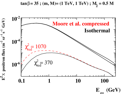
Figure 3: Positron flux dependence on the dark matter halo profile. A non–cuspy isothermal profile (continuous line) and the very cuspy Moore et al. profile with adiabatic compression (dashed line) are shown. Black upper curves show the background, and the signal plus background.

3.5 The PAMELA experiment

The PAMELA experiment has been launched recently into space. One of the PAMELA primary goals is the measurement of the cosmic positron spectrum up to 270 GeV [2]. The geometric acceptance in the standard trigger configuration is $\sim$ 20 $\mathrm{cm^{2}~{}sr}$. We consider in our analysis a three years mission and assume Gaussian statistics to determine the $\chi^{2}$.

Let us explain now how we can define that a positron signal arriving from the galactic halo will be distinguished effectively as a "signal" from the point of view of an experiment. We will mainly follow in this study the work by Lionetto, Morselli and Zdravkovic [27] and Hooper and Silk [28]. Let us call $\phi^{susy}$ the signal, $\phi^{bkg}$ the background, and $\phi^{tot}=\phi^{susy}+\phi^{bkg}$ the total flux which will be observed by PAMELA. We will divide our energy range between 1 to 500 GeV in 20 energy bins (N=20) logarithmically evenly spaced. For the discrimination between the signal and the background, we calculate the reduced $\chi^{2}$, $\chi^{2}_{\mathrm{red}}$:

$$\chi^{2}_{red}=\frac{1}{N}\sum_{n=0}^{N}\frac{(E_{n}^{2}\phi^{tot}_{n}-E_{n}^{2}\phi^{bkg}_{n})^{2}}{(\sigma_{n})^{2}}\ ,$$ (3.19)

where $\sigma_{n}$ is the error, assuming Gaussian statistic, on the measured value of the flux multiplied by $E_{n}^{2}$. For a "discovery signal", we request the condition $\chi^{2}_{red}>1.$

It is easy to check that this $\sigma_{n}$, for a given $E_{n}$, can be expressed as :

$$\sigma_{n}=\sqrt{\frac{E_{n}^{2}(E_{n}^{2}\phi^{tot})}{AT}}\ ,$$ (3.20)

where A is the geometrical factor or acceptance of the experiment mentioned above, and $T$ is the exposure time (3 years in our study). This means that a signal at one $\sigma$ in one energy bin $E_{n}$ will give us N hits in the range $N\pm\sqrt{N}$ after T seconds (Gaussian law).

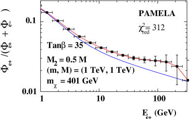
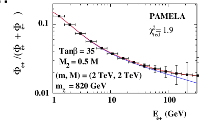
Figure 4: PAMELA expectations for positrons in the non–universal case $f)$ $M_{2}=0.5M$ with tan$\beta=35$, $A=0$, $m=1$ TeV, $M=1$ TeV (left) and $m=2$ TeV $M=2$ TeV (right), corresponding to a neutralino mass of $m_{\chi}=401$ GeV and $m_{\chi}=820$ GeV, respectively. The boost factor $BF$ has been set to 5 in an isothermal profile. The error bars shown are those projected for the PAMELA experiment after 3 years of observation. The lower (blue) line is the background–only prediction. The reduced $\chi^{2}$ is 312 in the first case giving a signal clearly distinguishable from the background whereas $\chi^{2}_{\mathrm{r}ed}$ is only 1.9 in the second case and gives a good fit of the background.

To illustrate the discussion we show in Fig. 4 the signal that we can expect for two different points in the non–universal SUGRA parameter space (in particular for the case $f)$ $M_{2}=0.5M$ in Eq. (2.4)). Let us remark that in addition to the propagation effects, as positrons approach the solar system, their interactions with the solar wind and magnetosphere can become important. These effects are called solar modulation. Alternatively, if one assumes that the effects of solar modulation are charge-sign independent, their impact can be removed considering the ratio of positrons to positrons plus electrons at a given energy rather than the positron flux alone. This quantity, the so-called $positron$ $fraction$ is often used to minimize the uncertainties associated with modelling the impact of solar modulation. As we can convert the fluxes to positron fractions by using fluxes of background positrons and electrons given by the Eqs. (3.5)-(3.7), we can replace the number of events used in Eq. (3.19) with ratios of positrons to positrons$+$electrons to reduce the effects of solar modulation in our results. Because there are substantially more electrons than positrons observed, we can assume that there are negligible errors associated with the electron flux.

4 The gamma–rays in the Galaxy

4.1 The flux

The spectrum of gamma–rays generated in dark matter annihilation and coming from a direction forming an angle $\psi$ with respect to the galactic center is

$$\Phi_{\gamma}(E_{\gamma},\psi)=\sum_{i}\frac{dN_{\gamma}^{i}}{dE_{\gamma}}\langle\sigma_{i}v\rangle\frac{1}{8\pi m_{\chi}^{2}}\int_{line\ of\ sight}\rho^{2}\ dl\ ,$$ (4.21)

where the discrete sum is over all dark matter annihilation channels, $dN_{\gamma}^{i}/dE_{\gamma}$ is the differential gamma–ray yield, $\langle\sigma_{i}v\rangle$ is the annihilation cross section averaged over its velocity distribution, and $\rho$ is the dark matter density.

	a (kpc)	$\alpha$	$\beta$	$\gamma$	$\bar{J}(10^{-5}{\rm sr})$
NFW	20	1	3	1	$1.264\times 10^{4}$
$\rm{NFW_{c}}$	20	0.8	2.7	1.45	$1.205\times 10^{7}$
Moore et al.	28	1.5	3	1.5	$5.531\times 10^{6}$
$\rm{Moore_{c}}$	28	0.8	2.7	1.65	$5.262\times 10^{8}$

Table 1: NFW and Moore et al. density profiles without and with adiabatic compression ($\rm{NFW}_{c}$ and $\rm{Moore_{c}}$ respectively) with the corresponding parameters, and values of $\bar{J}(\Delta\Omega)$.

It is customary to rewrite Eq. (4.21) introducing the dimensionless quantity $J$ (which depends only on the dark matter distribution):

$$J(\psi)=\frac{1}{8.5~{}\mathrm{kpc}}\left(\frac{1}{0.3~{}\mathrm{GeV/cm^{3}}}\right)^{2}\int_{line\ of\ sight}\rho^{2}(r(l,\psi))\ dl\ .$$ (4.22)

After having averaged over a solid angle, $\Delta\Omega$, the gamma–ray flux can now be expressed as

$$\Phi_{\gamma}(E_{\gamma}) = 0.94\times 10^{-13}\ \mathrm{cm^{-2}\ s^{-1}\ GeV^{-1}\ sr^{-1}}$$ (4.23)

$$\times \mbox{}\sum_{i}\frac{dN_{\gamma}^{i}}{dE_{\gamma}}\left(\frac{\langle\sigma_{i}v\rangle}{10^{-29}{\mathrm{cm^{3}s^{-1}}}}\right)\left(\frac{100~{}\mathrm{GeV}}{m_{\chi}}\right)^{2}{\overline{J}}(\Delta\Omega)\Delta\Omega\ .$$

The value of $\overline{J}(\Delta\Omega)\Delta\Omega$ depends crucially on the dark matter distribution. The different profiles that have been proposed in the literature can be parameterised as

$$\rho(r)=\frac{\rho_{0}[1+(R_{0}/a)^{\alpha}]^{(\beta-\gamma)/\alpha}}{(r/R_{0})^{\gamma}[1+(r/a)^{\alpha}]^{(\beta-\gamma)/\alpha}}\ ,$$ (4.24)

where $\rho_{0}$ is the local (solar neighborhood) halo density and $a$ is a characteristic length. Although we will use $\rho_{0}=0.3$ GeV/cm³ throughout the paper, since this is just a scaling factor in the analysis, modifications to its value can be straightforwardly taken into account in the results. N–body simulations suggest a cuspy inner region of dark matter halo with a distribution where $\gamma$ generally lies in the range 1 (NFW profile [29]) to 1.5 (Moore et al. profile [30]), producing a profile with a behaviour $\rho(r)\propto r^{-\gamma}$ at small distances. Over a solid angle of $10^{-5}$ sr, such profiles can lead to $\overline{J}(\Delta\Omega)\sim 10^{4}$ to $10^{7}$. Moreover, if we take into account the baryon distribution in the Galaxy, we can predict even more cuspy profiles with $\gamma$ in the range 1.45 to 1.65 ($\overline{J}(\Delta\Omega)\sim 10^{7}-10^{8}$) through the adiabatic compression process (see the study of Refs. [32, 12]). We summarize the parameters used in our study and the values of $\bar{J}$ for each profile in table 1. It is worth noticing here that we are neglecting the effect of clumpiness, even though other studies showed that, depending upon assumptions on the clumps distribution, in principle an enhacement of a factor 2 to 10 is possible [26]. Thus our predictions below for GLAST of the gamma-ray flux from the galactic center from dark matter pair annihilations, are conservative in this respect.

4.2 The background

HESS [5] has recently measured the gamma–ray spectrum from the galactic center in the range of energy $\sim$ [160 GeV–10 TeV]. The collaboration claim that the data are fitted by a power–law $F(E)=F_{0}~{}E_{\mathrm{TeV}}^{-\alpha}$, with a spectral index $\alpha=2.21\pm 0.09$ and $F_{0}=(2.50\pm 0.21)\times 10^{-8}~{}\mathrm{cm^{-2}~{}s^{-1}~{}TeV^{-1}}$ The data were taken during the second phase of the measurement (July–August, 2003) with a $\chi^{2}$ of 0.6 per degree of freedom. Because of the constant slope power–law observed by HESS, it results possible but difficult to conciliate such a spectrum with a signal from dark matter annihilation [12, 33]. Indeed, final particles (quarks, leptons or gauge bosons) produced through annihilations give rise to an spectrum with a continuously changing slope. Several astrophysical models have been proposed in order to match the HESS data [34]. In the present study we consider the astrophysical background for gamma–ray detection as the one extrapolated from the HESS data with a continuous power–law over the energy range of interest ($\approx$ 1 – 300 GeV). As was recently underlined in [7], GLAST sensitivity is affected by the presence of such an astrophysical source. Note that neutralino masses obtained in our parameter space $\lesssim 1$ TeV avoid any conflict with the observations of HESS.

In addition, we have also taken into account the EGRET data [4] in our background at energies below 10 GeV, as they can affect the sensitivity of the analysis. Indeed, the extrapolation of the gamma–ray fluxes measured by HESS down to energies as low as 1 GeV is likely to be an underestimation of the gamma–ray background in the galactic center, as EGRET measurements are one to two orders of magnitude higher than the HESS extrapolation. We have decided then to take as our background an interpolation between the HESS extrapolation and the EGRET data below 10 GeV to stay as conservative as possible in evaluating the gamma–ray background.

4.3 The GLAST experiment

The space–based gamma–ray telescope GLAST [8] is scheduled for launch in 2007 for a five years mission. It will perform an all-sky survey covering a large energy range ($\approx$ 1 – 300 GeV). With an effective area and angular resolution on the order of $10^{4}~{}\mathrm{cm^{2}}$ and $0.1^{o}$ ($\Delta\Omega\sim 10^{-5}$ sr) respectively, GLAST will be able to point and analyze the inner center of the Milky Way ($\sim 7$ pc).

In Fig. 5 we show the ability of GLAST to identify a signal from dark matter annihilation in the non–universal case $f)$ $M_{2}=0.5M$ with $\tan\beta=35$ for ($m=500$ GeV, $M=500$ GeV) and ($m=2$ TeV, $M=2$ TeV) giving a neutralino mass of 185.4 GeV and 820 GeV respectively. Concerning the requested condition on the $\chi^{2}_{red}$ for a signal discovery, we have used an analysis similar to the one considered in the case of positron detection with the PAMELA experiment in section 3.5, with a three years mission run. The error bars shown are projected assuming Gaussian statistic, and we adopt a power–law background extrapolated from the HESS data. We find that with a $\chi^{2}_{red}$ of 134, GLAST would potentially be able to detect dark matter annihilation radiation from a neutralino of mass 185.4 GeV, whereas with a $\chi^{2}_{red}$ of 0.02, a signal coming from a neutralino of mass 820 GeV will be below its sensitivity.

Figure 5: GLAST expectations for gamma–ray fluxes in the non–universal case $f)$ $M_{2}=0.5M$ with tan$\beta=35$, $A=0$, $m=500$ GeV, $M=500$ GeV (left) and $m=2$ TeV $M=2$ TeV (right), corresponding to a neutralino mass of $m_{\chi}=185.4$ GeV and 820 GeV, respectively. A NFW profile is used in both cases. The error bars shown are those projected for the GLAST experiment after 3 years of observation. The lower (blue) line is the background–only prediction. The reduced $\chi^{2}$ is 134 in the first case giving a signal clearly distinguishable from the background, whereas it is only 0.02 in the second case and gives a very good fit of the background.

5 Discussion

We have plotted in Fig. 6 the isocontour $\chi_{red}^{2}=1$ for PAMELA and GLAST, each after three years of observations, in the six cases of Eq. (2.4), and in the SUGRA parameter space (m, M) for $\tan\beta=35$, $A=0$ and $\mu>0$. We have calculated it for boost factors between 1 and $10^{4}$, and three typical halo profiles, isothermal (ISO), NFW, and NFW with adiabatic compression (NFW_c). We have taken into account in the computation the astrophysical and experimental constraints discussed in section 2.2. In particular, the brown-dark region is excluded by the experimental constraints and the stau as the lightest SUSY particle. The region to the right of the black dashed line corresponds to $a^{\rm SUSY}_{\mu}<7.1\times 10^{-10}$, and would be excluded by $e^{+}e^{-}$ data. The region between thick and thin solid contours fulfils $0.1\leq\Omega_{\tilde{\chi}_{1}^{0}}h^{2}\leq 0.3$ (the thick contour indicates the WMAP range $0.094<\Omega_{\tilde{\chi}_{1}^{0}}h^{2}<0.129$). Notice however that we did not rescale the fluxes according to the cosmological abundance, since this procedure would affect photon and positron in the same way and our work focuses on the comparison between the two kinds of detection. As usually discussed in the literature, for points with relic density away from WMAP values, scenarios with non-thermal production or dilution can be invoked to accomodate the abundance of neutralinos.

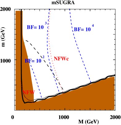
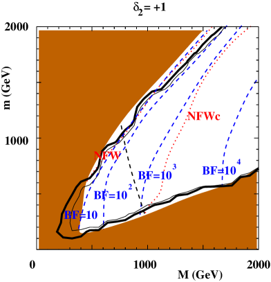
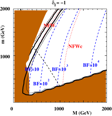
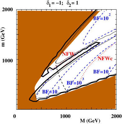
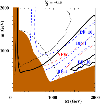
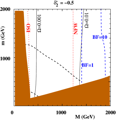
Figure 6: The isocontour $\chi_{red}^{2}=1$ for PAMELA (blue–dashed lines) and GLAST (red–dotted lines) for different kinds of halo profiles and boost factors, each after three years of observations, for tan$\beta=35$, $A_{0}=0$ and sign($\mu$) $>$ 0.

We clearly see in the figure that the parameter space of mSUGRA will be reachable only in astrophysical scenarios where the halo profile is very cuspy, like NFW_c (recall that this profile is also very similar to a Moore et al. profile without compression), or very clumpy with $BF\gtrsim$ 100. Notice in this sense that for a given $BF$ (halo profile), the region to the right of that blue-dashed (red-dotted) line will correspond to $\chi_{red}^{2}<1$, and therefore no observation. These results are in accordance with a similar study made in the framework of mSUGRA for the antiproton detection [27]. In case b), non–universality in $m_{H_{2}}$ ($\delta_{2}>0$) increase the Higgsino fraction of the neutralino: the annihilation process through $Z$ exchange is enhanced, permitting observations in NFW–type profiles or $BF\sim$ 10. Cases c) and d) are similar in the sense that the non-universality for $m_{H_{1}}$ ($\delta_{1}<0$) open a broad region of $A-$pole, increasing the gamma ray and positron fluxes through $\chi\chi\xrightarrow{A}f\overline{f}$, favored in high tan$\beta$ regimes. Profiles even less cuspy than NFW and boost factor $\lesssim$ 10 could be sufficient for an observation by GLAST or PAMELA. The phenomenon is even more spectacular in case e) where the non–universality in the gluino sector, $M_{3}$ ($\delta_{3}^{\prime}<0$), acts on $\mu$ and $m_{A}$ through the RGEs. As a consequence, the $A-$pole region is broader and allows observations even for $BF\sim 1$. In case f), the neutralino in mainly Wino and then annihilation to positrons is favored (through $W^{\pm}$ final states). In this scenario, a clumpy profile with a boost factor of about 1 would be comparable with a cuspy NFW profile. Unfortunatly, the amount of relic density in either cases is not sufficient to account for the WMAP results. As a conclusion, we can say that generically, GLAST and PAMELA will have similar discovery prospects for a NFW profile and $BF\sim 10$, or for a NFW_c profile and $BF\sim 1000$. Obviously, a boost factor as large as the latter is unrealistic, and in the case of halo models with adiabatic compression PAMELA cannot really be competitive with GLAST.

6 Conclusions

We have studied the indirect detection of neutralino dark matter using positrons and gamma rays from its annihilation in the galactic halo. Considering the HESS data as the spectrum constituting the gamma–ray background, we have compared the prospects for the experiments GLAST and PAMELA in a general SUGRA framework with non–universal soft gaugino and scalar masses. We have shown that with a clumpiness (boost) factor of about 10, PAMELA will be competitive with GLAST for a typical NFW cuspy profile. However, for the case of a NFW compressed profile, PAMELA cannot be competitive with GLAST since an unrealistic clumpiness factor of about 1000 would be necessary. For the future, it would be interesting to compile all the detection modes (antiproton, deuteron, positron and gamma rays) in order to carry out a complete analysis of the parameter space in a general SUGRA framework [9].

Acknowledgements

We thank Igor Moskalenko and Andrew Strong for their friendly collaboration during this work. We are also grateful to Pierre Salati and Julien Lavalle for having shared with us their knowledge about the propagation of positrons in our Galaxy. The authors want specially to thank warmly Aldo Morselli and Andrea Lionetto for their help and discussions on theoretical and experimental issues concerning GLAST and PAMELA.

The work of Y.M. was sponsored by the PAI programm PICASSO under contract PAI–10825VF. The work of C.M. was supported in part by the Spanish DGI of the MEC under Proyectos Nacionales BFM2003-01266 and FPA2003-04597 and under Acción Integrada Hispano-Francesa HF-2005-0005; by the Comunidad de Madrid under Ayudas de I+D S-0505/ESP-0346; and also by the European Union under the RTN program MRTN-CT-2004-503369, and under the ENTApP Network of the ILIAS project RII3-CT-2004-506222. The work of E.N. was supported by the I.I.S.N. and the Belgian Federal Science Policy (return grant and IAP 5/27).

References

- [1] For recent reviews, see: C. Munoz, ‘Dark matter detection in the light of recent experimental results’, Int. J. Mod. Phys.A19 (2004) 3093 [arXiv:hep-ph/0309346]; G. Bertone, D. Hooper and J. Silk, ‘Particle dark matter: Evidence, candidates and constraints’, Phys. Rept. 405 (2005) 279 [arXiv:hep-ph/0404175].
- [2] Y. I. Stozhkov et al. [PAMELA Collaboration], ‘About separation of hadron and electromagnetic cascades in the PAMELA calorimeter’, Int. J. Mod. Phys. A20 (2005) 6745; P. Picozza and A. Morselli, ‘The science of PAMELA space mission,’ arXiv:astro-ph/0604207.
- [3] F. Barao [AMS-02 Collaboration], ‘AMS: Alpha Magnetic Spectrometer on the International Space Station’, Nucl. Instrum. Meth. A535 (2004) 134.
- [4] S. D. Hunger et al. [EGRET Collaboration], ‘EGRET observations of the diffuse gamma-ray emission from the galactic plane’, Astrophys. J. 481 (1997) 205; H. A. Mayer-Hasselwander et al., ‘High-energy gamma-ray emission from the galactic center’ Astron. & Astrophys. 335 (1998) 161.
- [5] F. Aharonian et al. [HESS Collaboration], ‘Very high energy gamma–rays from the direction of Sagittarius A*’, Astron. Astrophys. 425 (2004) L13 [arXiv:astro-ph/0408145].
- [6] J. Albert et al. [MAGIC Collaboration], ‘Observation of gamma rays from the galactic center with the MAGIC telescope’, Astrophys. J. 638 (2006) L101 [arXiv:astro-ph/0512469].
- [7] G. Zaharijas and D. Hooper, ‘Challenges in detecting gamma–rays from dark matter annihilations in the galactic center’, arXiv:astro-ph/0603540.
- [8] N. Gehrels and P. Michelson, ‘GLAST: the next generation high-energy gamma–ray astronomy mission’, Astropart. Phys. 11 (1999) 277.
- [9] A. Lionetto, Y. Mambrini, A. Morselli, C. Munoz, E. Nezri, in preparation.
- [10] Y. Mambrini and C. Muñoz, ‘Gamma–ray detection from neutralino annihilation in non-universal SUGRA scenarios’, Astrop. Phys. 24 (2005) 208 [arXiv:hep-ph/0407158]; Y. Mambrini and C. Muñoz, ‘A comparison between direct and indirect dark matter search’, JCAP 10 (2004) 003 [arXiv:hep-ph/0407352].
- [11] H. Baer, A. Mustafayev, S. Profumo, A. Belyaev and X. Tata, ‘Direct, indirect and collider detection of neutralino dark matter in SUSY models with non-universal Higgs masses’, JHEP 07 (2005) 065 [arXiv:hep-ph/0504001]; H. Baer, A. Mustafayev, E. K. Park, S. Profumo and X. Tata, ‘Mixed higgsino dark matter from a reduced SU(3) gaugino mass: Consequences for dark matter and collider searches’, arXiv:hep-ph/0603197; H. Baer, A. Mustafayev, E. K. Park and S. Profumo, ‘Mixed Wino dark matter: Consequences for direct, indirect and collider detection’, JHEP 07 (2005) 046 [arXiv:hep-ph/0505227]; V. Bertin, E. Nezri and J. Orloff, ‘Neutralino dark matter beyond CMSSM universality,’ J. High Energy Phys. 02 (2003) 046 [arXiv:hep-ph/0210034]; A. Birkedal-Hansen and B. D. Nelson, ‘Relic neutralino densities and detection rates with nonuniversal gaugino masses,’ Phys. Rev. D67 (2003) 095006 [arXiv:hep-ph/0211071].
- [12] Y. Mambrini, C. Munoz, E. Nezri and F. Prada, ‘Adiabatic compression and indirect detection of supersymmetric dark matter’, JCAP 01 (2006) 010 [arXiv:hep-ph/0506204].
- [13] P. Gondolo, J. Edsjo, P. Ullio, L. Bergstrom, M. Schelke and E. A. Baltz, ‘DarkSUSY: Computing supersymmetric dark matter properties numerically’, arXiv:astro-ph/0406204; See also the web page http://www.physto.se/~edsjo/darksusy
- [14] A. Djouadi, J. L. Kneur and G. Moultaka, ‘SuSpect: a Fortran code for the supersymmetric and Higgs particle spectrum in the MSSM’, arXiv:hep-ph/0211331; See also the web page http://www.lpm.univ-montp2.fr:6714/~kneur/suspect.html.
- [15] G. W. Bennett et al. [Muon g-2 Collaboration], ‘Measurement of the negative muon anomalous magnetic moment to 0.7-ppm’, Phys. Rev. Lett. 92 (2004) 161802 [arXiv:hep-ex/0401008].
- [16] M. Davier, S. Eidelman, A. Hocker and Z. Zhang, ‘Updated estimate of the muon magnetic moment using revised results from annihilation’, Eur. Phys. J. C31 (2003) 503 [arXiv:hep-ph/0308213]; K. Hagiwara, A. D. Martin, D. Nomura and T. Teubner, ‘Predictions for of the muon and ’, Phys. Rev. D69 (2004) 093003 [arXiv:hep-ph/0312250]; J. F. de Troconiz and F. J. Yndurain, ‘The hadronic contributions to the anomalous magnetic moment of the muon’, Phys. Rev. D71 (2005) 073008 [arXiv:hep-ph/0402285].
- [17] S. Chen et al. [CLEO Collaboration], ‘Branching fraction and photon energy spectrum for ’, Phys. Rev. Lett. 87 (2001) 251807 [arXiv:hep-ex/0108032].
- [18] H. Tajima [BELLE Collaboration] ‘Belle B physics results’, Int. J. Mod. Phys. A17 (2002) 2967 [arXiv:hep-ex/0111037]; See also the web page http://wwwlapp.in2p3.fr/lapth/micromegas
- [19] G. Belanger, F. Boudjema, A. Pukhov and A. Semenov, ‘micrOMEGAs: a program for calculating the relic density in the MSSM’, Comput. Phys. Commun. 149 (2002) 103 [arXiv:hep-ph/0112278]; G. Belanger, F. Boudjema, A. Pukhov and A.G. Semenov, ‘MicrOMEGAs: Version 1.3’, [arXiv:hep-ph/0405253]; G. Belanger, F. Boudjema, A. Pukhov and A. Semenov, “micrOMEGAs2.0: A program to calculate the relic density of dark matter in a generic model,” arXiv:hep-ph/0607059.
- [20] A. W. Strong, I. V. Moskalenko and O. Reimer, ‘Diffuse Galactic continuum gamma–rays. A model compatible with EGRET data and cosmic-ray measurements’, Astrophys. J. 613 (2004) 962 [arXiv:astro-ph/0406254].
- [21] I. V. Moskalenko and A. W. Strong, ‘Production and propagation of cosmic-ray positrons and electrons’, Astrophys. J. 493 (1998) 694 [arXiv:astro-ph/9710124].
- [22] E. A. Baltz and J. Edsjo, ‘Positron propagation and fluxes from neutralino annihilation in the halo’, Phys. Rev. D59 (1999) 023511 [arXiv:astro-ph/9808243].
- [23] J. Lavalle, J. Pochon, P. Salati and R. Taillet, ‘Clumpiness of Dark Matter and Positron Annihilation Signal: Computing the odds of the Galactic Lottery’, arXiv:astro-ph/0603796.
- [24] J. Hisano, S. Matsumoto, O. Saito and M. Senami, “Heavy Wino-like neutralino dark matter annihilation into antiparticles,” Phys. Rev. D 73 (2006) 055004 [arXiv:hep-ph/0511118]; M. Asano, S. Matsumoto, N. Okada and Y. Okada, “Cosmic positron signature from dark matter in the littlest Higgs model with T-parity,” arXiv:hep-ph/0602157.
- [25] J. Silk and A. Stebbins, ‘Clumpy cold dark matter’, Astrophys. J. 411 (1993) 439.
- [26] L. Bergstrom, J. Edsjo, P. Gondolo and P. Ullio, ‘Clumpy neutralino dark matter’, Phys. Rev. D 59 (1999) 043506 [astro-ph/9806072].
- [27] A. M. Lionetto, A. Morselli and V. Zdravkovic, ‘Uncertainties of cosmic ray spectra and detectability of antiproton mSUGRA contributions with PAMELA’, JCAP 09 (2005) 010 [arXiv:astro-ph/0502406].
- [28] D. Hooper and J. Silk, ‘Searching for dark matter with future cosmic positron experiments’, Phys. Rev. D71 (2005) 083503 [arXiv:hep-ph/0409104].
- [29] J. F. Navarro, C. S. Frenk and S. D. M. White, ‘The Structure of Cold Dark Matter Halos’, Astrophys. J. 462 (1996) 563 [arXiv:astro-ph/9508025]; J. F. Navarro, C. S. Frenk and S. D. M. White, ‘A Universal Density Profile from Hierarchical Clustering’, Astrophys. J. 490 (1997) 493 [arXiv:astro-ph/9611107].
- [30] B. Moore, S. Ghigna, F. Governato, G. Lake, T. Quinn, J. Stadel and P. Tozzi, ‘Dark matter substructure within galactic halos’, Astrophys. J. 524 (1999) L19.
- [31] G. Gentile, P. Salucci, U. Klein, D. Vergani and P. Kalberla, MNRAS 351 (2004) 903 [arXiv:astro-ph/0403154].
- [32] F. Prada, A. Klypin, J. Flix, M. Martinez and E. Simonneau, ‘Astrophysical inputs on the SUSY dark matter annihilation detectability’, arXiv:astro-ph/0401512; G. Bertone and D. Merritt, ‘Dark matter dynamics and indirect detection’, Mod. Phys. Lett. A20 (2005) 1021 [arXiv:astro-ph/0504422]; G. Bertone and D. Merritt, ‘Time-Dependent Models for Dark Matter at the Galactic Center’, Phys. Rev. D72 (2005) 103502 [arXiv:astro-ph/0501555]. E. Athanassoula, F. S. Ling and E. Nezri, ‘Halo geometry and dark matter annihilation signal’, Phys. Rev. D72, 083503 (2005) [arXiv:astro-ph/0504631].
- [33] S. Profumo, ‘TeV gamma–rays and the largest masses and annihilation cross sections of neutralino dark matter’, Phys. Rev. D72 (2005) 103521 [arXiv:astro-ph/0508628]; D. Hooper, I. de la Calle Perez, J. Silk, F. Ferrer and S. Sarkar, ‘Have atmospheric Cerenkov telescopes observed dark matter?’, JCAP 09 (2004) 002 [arXiv:astro-ph/0404205].
- [34] F. Aharonian and A. Neronov, ‘High energy gamma–rays from the massive black hole in the galactic center’, Astrophys. J. 619 (2005) 306 [arXiv:astro-ph/0408303]; A. Atoyan and C. D. Dermer, ‘TeV emission from the galactic center black-hole plerion’, Astrophys. J. 617 (2004) L123 [arXiv:astro-ph/0410243].