1 Introduction

The impressive experimental evidence of neutrino masses [1] has lead to the first clear signal of physics beyond the standard model (SM). One of the simplest extensions of the SM that allows to naturally explain the smallness of the neutrino masses (without excessively tiny Yukawa couplings) consists in incorporating right-handed Majorana neutrinos, and imposing a seesaw mechanism for the neutrino mass generation [2, 3]. The seesaw mechanism offers in addition the interesting possibility of baryogenesis via leptogenesis [4]. Within the framework of leptogenesis, the observed baryon asymmetry of the Universe (BAU) is explained by the out-of-equilibrium decays of the same heavy right-handed neutrinos which are responsible for the suppression of the light neutrino masses. The scale of new physics is naturally introduced by the heavy right-handed neutrino masses which, for the simplest case of just one right-handed neutrino, and assuming neutrino Yukawa couplings, $Y_{\nu}$, of $\mathcal{O}(1)$, typically lies close to $10^{14}$ GeV.

Supersymmetric (SUSY) extensions of the SM, including three right-handed neutrino superfields, are well motivated models which can accommodate a seesaw mechanism, and at the same time stabilise the hierarchy between the scale of new physics and the electroweak (EW) scale. One of the most striking phenomenological implications of SUSY seesaw models is the prediction of sizable rates for lepton flavour violating (LFV) processes [5]. Assuming $Y_{\nu}\approx\mathcal{O}(1)$ and that the scale of soft-SUSY breaking is of the order (or below) 1 TeV, the radiatively induced SUSY corrections driven by the neutrino Yukawa couplings lead to rates for the LFV observables which are many orders of magnitude larger than those expected from the SM seesaw. Even though this holds irrespective of the chosen mass pattern for the right-handed neutrinos, it has been shown that when compared to the degenerate case [6, 7] the hierarchical scenario leads to larger LFV rates, which may even be within the reach of current experimental bounds [8, 9, 10, 11, 12, 13, 14, 15, 16, 17, 18, 19, 20]. In this sense, the $l_{j}\to l_{i}\,\gamma$ and $l_{j}\to 3\,l_{i}$ ($i\neq j)$ lepton decay channels, as well as $\mu-e$ conversion in heavy nuclei, are among the most interesting processes [21]. Experimentally, the most promising decay is the $\mu\to e\,\gamma$ process, which exhibits the most stringent present bounds, and offers a significant improvement regarding the future sensitivity. Furthermore, in the presence of complex neutrino Yukawa couplings, one can also construct from the latter LFV decays interesting observables, which are sensitive to CP violation in the neutrino sector. For instance, one can build T- and P-odd asymmetries in $\mu\to e\,\gamma$ and $\mu\to 3\,e$ decays, which were addressed in [22, 23].

In addition to the large number of parameters of the minimal supersymmetric standard model (MSSM), the seesaw mechanism introduces 18 new parameters in the neutrino sector. As a first step to simplify the analysis of the LFV rates in a SUSY seesaw model, we choose to work in the so-called constrained MSSM (CMSSM), assuming universality of the soft-SUSY breaking parameters at the scale of gauge coupling unification, $M_{X}$. This allows to reduce the unknown parameters in the SUSY sector to the five usual parameters of a minimal supergravity (mSUGRA) framework. Moreover, regarding the neutrino sector, we will assume a hierarchical spectrum for both light and heavy neutrinos.

Among the various seesaw parameters, those connected to the light neutrino sector can in principle be derived from low-energy neutrino data, while those associated with the heavy neutrino sector, in particular the values of the masses, are à priori clearly unreachable. However, and given the fact that both light and heavy neutrinos enter in the determination of the LFV rates (via the Yukawa interactions), a powerful link between the low- and high-energy neutrino parameters can be obtained from these LFV processes. From the requirement of compatibility with both current LFV bounds and low-energy neutrino data, one can then extract information on the heavy neutrino sector, thus providing an indirect access to the heavy neutrino parameters. In the presence of additional CP phases (other than those associated to the light sector), and assuming that BAU is generated from thermal leptogenesis, one can obtain a further insight on the heavy neutrino parameters. More specifically, one can obtain a lower bound on the mass of the lightest right-handed neutrino, which in turn translates into lower mass bounds for the other heavy states.

Here we address the subject of how to extract information on the unknown SUSY-seesaw parameters from both the analysis of LFV decays and the requirement of successful BAU. As already said, we restrict ourselves to the scenario of hierarchical heavy neutrinos, which leads to the most interesting predictions. There are studies also addressing the same subject, within similar SUSY seesaw frameworks and hierarchical neutrino scenarios. In particular, some constraints on the heavy neutrino and SUSY sectors have been considered by [13, 14, 15, 16, 17, 18, 19, 20] and further implications regarding low-energy CP violating observables were studied in [22, 23, 24, 25]. In addition, it has been noticed that not only are the LFV branching ratios (BRs) sensitive to the heavy neutrino parameters, but there is also a potentially relevant role being played by the yet undetermined low-energy neutrino parameters. The latter include the overall light neutrino mass scale and CP violating phases. Concretely, the effects of this scale and of the two Majorana phases on the radiative LFV decays have been analysed in [26].

An even more intriguing situation occurs regarding the sensitivity of the LFV rates to $\theta_{13}$, which is our main interest here. Although it is not expected to be of relevance in the context of the LFV phenomenology, the few studies regarding the dependence of LFV rates on $\theta_{13}$ [15, 18] have revealed that, for some specific seesaw cases, the LFV muon decays indeed exhibit a strong sensitivity to this parameter. In particular, the dependence of the BR($\mu\to e\,\gamma$) on $\theta_{13}$ was noticed [15] in the context of SUSY grand unified theories (SUSY-GUTs), and in [18] within the CMSSM. In the latter, it was further emphasised that in addition to $\mu\to e\,\gamma$ other LFV decays as $\mu\to 3\,e$ are also very sensitive to $\theta_{13}$. Both these studies assumed a simple scenario where no additional mixing, other than that induced from the low-energy mixing angles $\theta_{ij}$, was present in the neutrino sector.

In this work we systematically explore the sensitivity of LFV processes to $\theta_{13}$ in a broader class of SUSY seesaw scenarios, with different possibilities for the mixing in the neutrino sector, and we incorporate in our analysis the requirement of BAU via thermal leptogenesis. Specifically, we conduct a comprehensive and comparative study of the dependence on $\theta_{13}$ in all the following decay channels: $\mu^{-}\to e^{-}\,\gamma$, $\mu^{-}\to e^{-}\,e^{-}\,e^{+}$, $\tau^{-}\to e^{-}\,\gamma$, $\tau^{-}\to e^{-}\,e^{-}\,e^{+}$, $\tau^{-}\to\mu^{-}\,\gamma$ and $\tau^{-}\to\mu^{-}\,\mu^{-}\,\mu^{+}$. We will show here that various of these channels indeed offer interesting expectations regarding the sensitivity to $\theta_{13}$. In our analysis, we work in the context of a CMSSM extended by three right-handed neutrinos and their SUSY partners, and use the requirement of generating a successful BAU in order to constrain the explored seesaw parameter space. Our main motivation to perform the present study has been triggered by the potential measurement of $\theta_{13}$, as suggested by the experimental program of MINOS and OPERA, which claim a future experimental sensitive of $\theta_{13}\lesssim 8^{\circ}$ [27] and $\theta_{13}\lesssim 7^{\circ}$ [28, 29], respectively. With the advent of other experiments, like Double Chooz and T2K, the expected sensitivity will be further improved to $\theta_{13}\lesssim 4^{\circ}$ [30] and $\theta_{13}\lesssim 2^{\circ}$ [31]. An ambitious program to push the sensitivity to less than $1^{\circ}$ is envisioned by Neutrino Factory [32, 33] and/or Beta Beam [34, 35] facilities.

Our ultimate goal is to explore the impact of a potential $\theta_{13}$ measurement on the LFV branching ratios, which together with the current and future experimental bounds (measurements) on the latter ratios, could lead to a better knowledge (determination) of the heavy neutrino parameters.

Our work is organised as follows. In Section 2, we present the SUSY seesaw scenario, describing the seesaw mechanism for the neutrino mass generation, and discussing how flavour mixing in the slepton and sneutrino sectors arises in this context. We further address the constraints on the seesaw parameters from the requirement of generating a successful BAU via thermal leptogenesis, and from imposing compatibility with experimental data on charged lepton electric dipole moments (EDMs). In Section 3, we explore in detail how the several parameters affect the theoretical predictions for the LFV rates, and whether the former can modify the sensitivity of a given LFV observable to $\theta_{13}$. Section 4 is devoted to the discussion of the hints on SUSY and seesaw parameters which can be derived from a potential measurement of $\theta_{13}$ and LFV branching ratios. Finally, our conclusions are summarised in Section 5.

2 LFV within the SUSY seesaw model

In what follows, we first present the SUSY seesaw scenario within the CMSSM, then proceed to describe how LFV processes arise in this framework and finally discuss the implications regarding BAU and charged lepton EDMs.

2.1 The SUSY seesaw scenario

The leptonic superpotential containing the relevant terms to describe a type-I SUSY seesaw is given by

$$W\,=\,\hat{N}^{c}\,Y_{\nu}\,\hat{L}\,\hat{H}_{2}\,+\,\hat{E}^{c}\,Y_{l}\,\hat{L}\,\hat{H}_{1}\,+\,\frac{1}{2}\,\hat{N}^{c}\,m_{M}\,\hat{N}^{c}\,,$$ (1)

where $\hat{N}^{c}$ is the additional superfield that contains the three right-handed neutrinos $\nu_{R_{i}}$ and their scalar partners $\tilde{\nu}_{R_{i}}$. The lepton Yukawa couplings $Y_{l,\nu}$ and the Majorana mass $m_{M}$ are $3\times 3$ matrices in lepton flavour space. From now on, we will assume that we are in a basis where $Y_{l}$ and $m_{M}$ are diagonal.

After EW symmetry breaking, the charged lepton and Dirac neutrino mass matrices can be written as

$$m_{l}\,=\,Y_{l}\,\,v_{1}\,,\quad\quad m_{D}\,=\,Y_{\nu}\,v_{2}\,,$$ (2)

where $v_{i}$ are the vacuum expectation values (VEVs) of the neutral Higgs scalars, with $v_{1(2)}=\,v\,\cos(\sin)\beta$ and $v=174$ GeV.

The $6\times 6$ neutrino mass matrix is given by

$$M^{\nu}\,=\,\left(\begin{array}[]{cc}0&m_{D}^{T}\\ m_{D}&m_{M}\end{array}\right)\,.$$ (3)

The eigenvalues of $M^{\nu}$ are the masses of the six physical Majorana neutrinos. In the seesaw limit, the three right-handed masses are much heavier than the EW scale, $m_{M_{i}}\,\gg\,v$, and one obtains three light and three heavy states, $\nu_{i}$ and $N_{i}$, respectively.

Block-diagonalisation of the neutrino mass matrix of Eq. (3), leads (at lowest order in the $(m_{D}/m_{M})^{n}$ expansion) to the standard seesaw equation for the light neutrino mass matrix,

$$m_{\nu}\,=\,-m_{D}^{T}m_{M}^{-1}m_{D}\,,$$ (4)

as well as the simpler relation for the heavy mass eigenstates, $m_{N}\,=\,m_{M}$. Since we are working in a basis where $m_{M}$ is diagonal, the heavy eigenstates are then given by

$$m_{N}^{\text{diag}}\,=\,m_{N}\,=\,\text{diag}\,(m_{N_{1}},m_{N_{2}},m_{N_{3}})\,.$$ (5)

The matrix $m_{\nu}$ can be diagonalised by the Maki-Nakagawa-Sakata unitary matrix $U_{\text{MNS}}$ [36, 37], leading to the following masses for the light physical states

$$m_{\nu}^{\text{diag}} \,=\,U_{\text{MNS}}^{T}\,m_{\nu}\,U_{\text{MNS}}\,=\,\text{diag}\,(m_{\nu_{1}},m_{\nu_{2}},m_{\nu_{3}})\,.$$ (6)

Here we use the standard parameterisation for $U_{\mathrm{MNS}}$ given by

$$U_{\text{MNS}}=\left(\begin{array}[]{ccc}c_{12}\,c_{13}&s_{12}\,c_{13}&s_{13}\,e^{-i\delta}\\ -s_{12}\,c_{23}\,-\,c_{12}\,s_{23}\,s_{13}\,e^{i\delta}&c_{12}\,c_{23}\,-\,s_{12}\,s_{23}\,s_{13}\,e^{i\delta}&s_{23}\,c_{13}\\ s_{12}\,s_{23}\,-\,c_{12}\,c_{23}\,s_{13}\,e^{i\delta}&-c_{12}\,s_{23}\,-\,s_{12}\,c_{23}\,s_{13}\,e^{i\delta}&c_{23}\,c_{13}\end{array}\right)\,.\,V\,,$$ (7)

with

$$V\,=\,\text{diag}\,(e^{-i\frac{\phi_{1}}{2}},e^{-i\frac{\phi_{2}}{2}},1)\,,$$ (8)

and $c_{ij}\equiv\cos\theta_{ij}$, $s_{ij}\equiv\sin\theta_{ij}$. $\theta_{ij}$ are the neutrino flavour mixing angles, $\delta$ is the Dirac phase and $\phi_{1,2}$ are the Majorana phases.

In view of the above, the seesaw equation (4) can be solved for $m_{D}$ as [10]

$$m_{D}\,=\,i\sqrt{m^{\text{diag}}_{N}}\,R\,\sqrt{m^{\text{diag}}_{\nu}}\,U^{\dagger}_{\text{MNS}}\,,$$ (9)

where $R$ is a generic complex orthogonal $3\times 3$ matrix that encodes the possible extra neutrino mixings (associated with the right-handed sector) in addition to the ones in $U_{\text{MNS}}$. $R$ can be parameterised in terms of three complex angles, $\theta_{i}$ $(i=1,2,3)$ as

$$R\,=\,\left(\begin{array}[]{ccc}c_{2}\,c_{3}&-c_{1}\,s_{3}\,-\,s_{1}\,s_{2}\,c_{3}&s_{1}\,s_{3}\,-\,c_{1}\,s_{2}\,c_{3}\\ c_{2}\,s_{3}&c_{1}\,c_{3}\,-\,s_{1}\,s_{2}\,s_{3}&-s_{1}\,c_{3}\,-\,c_{1}\,s_{2}\,s_{3}\\ s_{2}&s_{1}\,c_{2}&c_{1}\,c_{2}\end{array}\right)\,,$$ (10)

with $c_{i}\equiv\cos\theta_{i}$, $s_{i}\equiv\sin\theta_{i}$. Eq. (9) is a convenient means of parameterising our ignorance of the full neutrino Yukawa couplings, while at the same time allowing to accommodate the experimental data. Notice that it is only valid at the right-handed neutrino scales $m_{M}$, so that the quantities appearing in Eq. (9) are the renormalised ones, $m^{\text{diag}}_{\nu}\,(m_{M})$ and $U_{\text{MNS}}\,(m_{M})$.

We shall focus on the simplest scenario, where both the heavy and light neutrinos are hierarchical, and in particular we will assume a normal hierarchy,

$$m_{N_{1}}\,\ll\,m_{N_{2}}\,\ll\,m_{N_{3}}\,,$$

$$m_{\nu_{1}}\,\ll\,m_{\nu_{2}}\,\ll\,m_{\nu_{3}}\,.$$ (11)

The masses $m_{\nu_{2,3}}$ can be written in terms of the lightest mass $m_{\nu_{1}}$, and of the solar and atmospheric mass-squared differences as

$$m_{\nu_{2}}^{2}\,=\,\Delta m_{\text{sol}}^{2}\,+\,m_{\nu_{1}}^{2}\,,$$

$$m_{\nu_{3}}^{2}\,=\,\Delta m_{\text{atm}}^{2}\,+\,m_{\nu_{1}}^{2}\,.$$ (12)

Moving now to the s-spectrum, we encounter an enlarged slepton sector due to the inclusion of the SUSY partners of $\nu_{R_{i}}$, namely ${\tilde{\nu}}_{R_{i}}$. The soft-SUSY breaking Lagrangian for the slepton sector will also include new terms and parameters. In addition to the left- and right-handed soft-breaking masses, $m_{\tilde{L}}$, $m_{\tilde{E}}$, and trilinear couplings, $A_{l}$, for the charged sleptons, one now includes soft-breaking sneutrino masses, $m_{\tilde{M}}$, sneutrino trilinear couplings $A_{\nu}$, and the new bilinear parameter, $B_{M}$.

The universality conditions of the soft-SUSY breaking parameters at the high-energy scale $M_{X}$ (with $M_{X}\gg m_{M}$) for the full slepton sector then read as follows:

$$\left(m_{\tilde{L}}\right)^{2}_{ij}\,=\,\left(m_{\tilde{E}}\right)^{2}_{ij}\,=\,\left(m_{\tilde{M}}\right)^{2}_{ij}\,=\,M_{0}^{2}\,\delta_{ij}\,,\,\,$$

$$\left(A_{l}\right)_{ij}\,=\,A_{0}\,\left(Y_{l}\right)_{ij}\,,\,\,\left(A_{\nu}\right)_{ij}\,=\,A_{0}\,\left(Y_{\nu}\right)_{ij}\,,$$ (13)

where $M_{0}$ and $A_{0}$ are the universal scalar soft-breaking mass and trilinear coupling of the CMSSM, and $i,j$ denote lepton flavour indices, with $i,j=1,2,3$. Here, we choose $M_{X}$ to be the gauge coupling unification scale. The extended CMSSM is further specified by the universal gaugino mass, $M_{1/2}$, the ratio of the Higgs VEVs, $\tan\beta$, and the sign of the bilinear $\mu$-parameter ($\text{sign}\,\mu$).

The CMSSM predictions for the low-energy parameters are obtained by solving the full renormalisation group equations (RGEs), which must now include the appropriate equations and extra terms for the extended neutrino and sneutrino sectors. Due to the existence of intermediate scales $m_{M}$ introduced by the seesaw mechanism, the running must be carried in two steps. The full set of equations is first run down from $M_{X}$ to $m_{M}$. At the seesaw scales, the right-handed neutrinos as well as their SUSY partners decouple, and the new RGEs (without the equations and terms for $\nu_{R}$ and $\tilde{\nu}_{R}$) are then run down from $m_{M}$ to the EW scale, where the couplings and mass matrices are finally computed.

2.2 Lepton flavour violating decays

In the present study, and since we work within the CMSSM, all LFV originates solely from the neutrino Yukawa couplings. For the LFV process that we are interested in, the flavour mixing in the neutrino sector is transmitted to the charged lepton sector via radiative corrections involving $Y_{\nu}$. These corrections can be important since, due to the Majorana nature of the neutrinos, the Yukawa couplings may be sizable (as large as $\mathcal{O}(1)$). In particular, we will consider here the following LFV muon and tau decays: $\mu\to e\gamma$, $\tau\to\mu\gamma$, $\tau\to e\gamma$, $\mu\to 3\,e$, $\tau\to 3\,e$ and $\tau\to 3\,\mu$.

Under the requirement that at the seesaw scales ($m_{M}$) $Y_{\nu}$ satisfies Eq. (9), the running from $M_{X}$ down to the EW scale will induce flavour mixing in the low-energy charged slepton squared mass matrix, $M_{\tilde{l}}^{2}$, whose $LL$, $RR$, $LR$ and $RL$ elements are given by

$$M_{LL}^{ij\,2} \,=\,m_{\tilde{L},ij}^{2}\,+\,v_{1}^{2}\,\left(Y_{l}^{\dagger}\,Y_{l}\right)_{ij}\,+\,m_{Z}^{2}\,\cos 2\beta\,\left(-\frac{1}{2}\,+\,\sin^{2}\theta_{W}\right)\,\delta_{ij}\,,$$

$$M_{RR}^{ij\,2} \,=\,m_{\tilde{E},ij}^{2}\,+\,v_{1}^{2}\,\left(Y_{l}^{\dagger}\,Y_{l}\right)_{ij}\,-\,m_{Z}^{2}\,\cos 2\beta\,\sin^{2}\theta_{W}\,\delta_{ij}\,,$$

$$M_{LR}^{ij\,2} \,=\,v_{1}\,\left(A_{l}^{ij}\right)^{*}\,-\,\mu\,Y_{l}^{ij}\,v_{2}\,,$$

$$M_{RL}^{ij\,2} \,=\,\left(M_{LR}^{ji\,2}\right)^{*}\,,$$ (14)

with $m_{Z}$ the $Z$-boson mass and $\theta_{W}$ the weak mixing angle. Below $m_{M}$, the right-handed sneutrinos decouple, and the low-energy sneutrino mass eigenstates are dominated by the $\tilde{\nu}_{L}$ components [38]. Thus, the sneutrino flavour mixing is confined to the left-handed sector, and described by the following $3\times 3$ matrix:

$$M_{\tilde{\nu}}^{ij\,2}\,=\,m_{\tilde{L},ij}^{2}+\frac{1}{2}\,m_{Z}^{2}\,\cos 2\beta\,\delta_{ij}\,.$$ (15)

The physical masses and states are obtained by diagonalising the previous mass matrices, leading to

$${M_{\tilde{l}}^{2}}^{\text{diag}} \,=\,R^{l}\,M_{\tilde{l}}^{2}\,R^{l\,\dagger}\,=\,\text{diag}\,(m_{\tilde{l}_{1}}^{2},..,m_{\tilde{l}_{6}}^{2})\,,$$

$${M_{\tilde{\nu}}^{2}}^{\text{diag}} \,=\,R^{\nu}\,M_{\tilde{\nu}}^{2}\,R^{\nu\,\dagger}\,=\,\text{diag}\,(m_{\tilde{\nu}_{1}}^{2},\,m_{\tilde{\nu}_{2}}^{2},\,m_{\tilde{\nu}_{3}}^{2})\,,$$ (16)

where $R^{l,\nu}$ are unitary rotation matrices.

The LFV ratios for the decay processes of our interest are obtained here via a full one-loop computation (and in terms of physical eigenstates), including all relevant SUSY diagrams.

For the radiative decays $l_{j}\to l_{i}\,\gamma$ ($i\neq j$), the branching ratios are given by

$$\text{BR}(l_{j}\to l_{i}\,\gamma)\,=\,\frac{e^{2}}{16\,\pi}\,\frac{m^{5}_{l_{j}}}{\Gamma_{l_{j}}}\,\left(|A_{2}^{L}|^{2}\,+\,|A_{2}^{R}|^{2}\right)\,,$$ (17)

where ${\Gamma_{l_{j}}}$ is the total lepton width, and the form factors $A_{2}^{L,R}$ receive contributions from two types of diagrams, sneutrino-chargino loops and charged slepton-neutralino loops. These BRs were computed in Ref. [5, 6]. We will use in our analysis the explicit formulae for the $|A_{2}^{L,R}|$ form factors as in Ref. [18].

Regarding the LFV decays into three leptons, $l_{j}\to 3\,l_{i}$, the one-loop computation was presented in [6], and later revised and completed in [18]. The latter work included the full set of SUSY one-loop contributing diagrams, namely photon-, $Z$-, and Higgs-penguins, as well as box diagrams. As shown by the explicit computation of [18], the dominant contribution is clearly coming from the photon-penguin diagrams and, more specifically, from the same form factors $A_{2}^{L,R}$ as in the case of the radiative decays. This is valid even in the case of very large $\tan\beta$ where the Higgs-penguin diagrams, although enhanced, induce contributions which are still many orders of magnitude below those associated with the photon-penguins. Therefore, the BR for the $l_{j}\to 3\,l_{i}$ decays can be approximated by the simple expression,

$$\text{BR}(l_{j}\to 3l_{i})\,=\,\frac{\alpha}{3\,\pi}\,\left(\log\frac{m_{l_{j}}^{2}}{m_{l_{i}}^{2}}\,-\,\frac{11}{4}\right)\,\times\,\text{ BR}(l_{j}\to l_{i}\,\gamma)\,,$$ (18)

where $\alpha$ is the electromagnetic coupling constant. However, and although we have verified that this is indeed a very good approximation, we use in the present analysis the full one-loop formulae for the BR($l_{j}\to 3l_{i}$) from Ref. [18].

Finally, and regarding the estimation of the low-energy parameters, we consider the full 2-loop RGE running, except for the neutrino sector which is treated at the 1-loop level. Nevertheless, for the forthcoming discussion, it will be clarifying and interesting to compare the full results with the simplified estimation which is obtained within the leading logarithmic approximation (LLog). In the latter framework, the RGE generated flavour mixing in the slepton sector is summarised by the following logarithmic contributions,

$$(\Delta m_{\tilde{L}}^{2})_{ij} \,=\,-\frac{1}{8\,\pi^{2}}\,(3\,M_{0}^{2}+A_{0}^{2})\,(Y_{\nu}^{\dagger}\,L\,Y_{\nu})_{ij}\,,$$

$$(\Delta A_{l})_{ij} \,=\,-\frac{3}{16\,\pi^{2}}\,A_{0}\,Y_{l_{i}}\,(Y_{\nu}^{\dagger}\,L\,Y_{\nu})_{ij}\,,$$

$$(\Delta m_{\tilde{E}}^{2})_{ij} \,=\,0\,\,;\,L_{kl}\,\equiv\,\log\left(\frac{M_{X}}{m_{M_{k}}}\right)\,\delta_{kl}\,,$$ (19)

which are originated by the running from $M_{X}$ to the right handed mass scales $m_{M_{i}}$, $i=1,2,3$. The matrix elements $(Y_{\nu}^{\dagger}LY_{\nu})_{ij}$ in Eq. (2.2) can be simply written in terms of the parameterisation of Eqs. (5-10). In particular, we obtain

$$v_{2}^{2}\,(Y_{\nu}^{\dagger}\,L\,Y_{\nu})_{21}\,=\,$$

$${L_{33}}\,{m_{N_{3}}}\,\left[{c_{13}}\,\left(e^{\frac{i}{2}\,{{\phi}_{1}}}\,{\sqrt{{m_{\nu_{1}}}}}\,{c_{12}}\,{s_{2}}+e^{\frac{i}{2}\,{{\phi}_{2}}}\,{\sqrt{{m_{\nu_{2}}}}}\,{c_{2}}\,{s_{1}}\,{s_{12}}\right)+e^{i\,\delta}\,{\sqrt{{m_{\nu_{3}}}}}\,{c_{1}}\,{c_{2}}\,{s_{13}}\right]\,$$

$$\qquad\left[{\sqrt{{m_{\nu_{3}}}}}\,{c_{1}}\,{c_{2}}\,{c_{13}}\,{s_{23}}-e^{-\frac{i}{2}\,{{\phi}_{1}}}{{\sqrt{{m_{\nu_{1}}}}}\,{s_{2}}\,\left({c_{23}}\,{s_{12}}+e^{i\,\delta}\,{c_{12}}\,{s_{13}}\,{s_{23}}\right)}\right.$$

$$\qquad+\left.e^{-\frac{i}{2}\,{{\phi}_{2}}}{{\sqrt{{m_{\nu_{2}}}}}\,{c_{2}}\,{s_{1}}\,\left({c_{12}}\,{c_{23}}-e^{i\,\delta}\,{s_{12}}\,{s_{13}}\,{s_{23}}\right)}\right]$$

$$+{L_{22}}\,m_{N_{2}}\,\left[e^{\frac{i}{2}\,{{\phi}_{1}}}\,{\sqrt{{m_{\nu_{1}}}}}\,{c_{2}}\,{c_{12}}\,{c_{13}}\,{s_{3}}+e^{\frac{i}{2}\,{{\phi}_{2}}}\,{\sqrt{{m_{\nu_{2}}}}}\,{c_{13}}\,\left({c_{1}}\,{c_{3}}-{s_{1}}\,{s_{2}}\,{s_{3}}\right)\,{s_{12}}\right.$$

$$\left.\qquad-e^{i\,\delta}\,{\sqrt{{m_{\nu_{3}}}}}\,\left({c_{3}}\,{s_{1}}+{c_{1}}\,{s_{2}}\,{s_{3}}\right)\,{s_{13}}\right]\,$$

$$\qquad\left[-{\sqrt{{m_{\nu_{3}}}}}\,{c_{13}}\,\left({c_{3}}\,{s_{1}}+{c_{1}}\,{s_{2}}\,{s_{3}}\right)\,{s_{23}}-e^{-\frac{i}{2}\,{{\phi}_{1}}}{{\sqrt{{m_{\nu_{1}}}}}\,{c_{2}}\,{s_{3}}\,\left({c_{23}}\,{s_{12}}+e^{i\,\delta}\,{c_{12}}\,{s_{13}}\,{s_{23}}\right)}\right.$$

$$\left.\qquad+e^{-\frac{i}{2}\,{{\phi}_{2}}}{{\sqrt{{m_{\nu_{2}}}}}\,\left({c_{1}}\,{c_{3}}-{s_{1}}\,{s_{2}}\,{s_{3}}\right)\,\left({c_{12}}\,{c_{23}}-e^{i\,\delta}\,{s_{12}}\,{s_{13}}\,{s_{23}}\right)}\right]$$

$$+{L_{11}}\,m_{N_{1}}\,\left[e^{\frac{i}{2}\,{{\phi}_{1}}}\,{\sqrt{{m_{\nu_{1}}}}}\,{c_{2}}\,{c_{3}}\,{c_{12}}\,{c_{13}}-e^{\frac{i}{2}\,{{\phi}_{2}}}\,{\sqrt{{m_{\nu_{2}}}}}\,{c_{13}}\,\left({c_{3}}\,{s_{1}}\,{s_{2}}+{c_{1}}\,{s_{3}}\right)\,{s_{12}}\right.$$

$$\qquad\left.+e^{i\,\delta}\,{\sqrt{{m_{\nu_{3}}}}}\,\left(-\left({c_{1}}\,{c_{3}}\,{s_{2}}\right)+{s_{1}}\,{s_{3}}\right)\,{s_{13}}\right]\,$$

$$\qquad\left[{\sqrt{{m_{\nu_{3}}}}}\,{c_{13}}\,\left(-\left({c_{1}}\,{c_{3}}\,{s_{2}}\right)+{s_{1}}\,{s_{3}}\right)\,{s_{23}}-e^{-\frac{i}{2}\,{{\phi}_{1}}}{{\sqrt{{m_{\nu_{1}}}}}\,{c_{2}}\,{c_{3}}\,\left({c_{23}}\,{s_{12}}+e^{i\,\delta}\,{c_{12}}\,{s_{13}}\,{s_{23}}\right)}\right.$$

$$\left.\qquad-e^{-\frac{i}{2}\,{{\phi}_{2}}}{{\sqrt{{m_{\nu_{2}}}}}\,\left({c_{3}}\,{s_{1}}\,{s_{2}}+{c_{1}}\,{s_{3}}\right)\,\left({c_{12}}\,{c_{23}}-e^{i\,\delta}\,{s_{12}}\,{s_{13}}\,{s_{23}}\right)}\right]\,.$$ (20)

The above is the relevant matrix element for the $\mu\to e\gamma$ and $\mu\to 3e$ decays, which will be the most emphasised in the present work. Correspondingly, the expression for the $(Y_{\nu}^{\dagger}\,L\,Y_{\nu})_{32}$ ($(Y_{\nu}^{\dagger}\,L\,Y_{\nu})_{31}$) matrix element, omitted here for brevity, is the relevant one with respect to $\tau\to\mu\gamma$ and $\tau\to 3\,\mu$ ($\tau\to e\gamma$ and $\tau\to 3\,e$) decays.

Since the dominant contribution to the $\mu\to e\gamma$ decay stems from the RGE induced flavour mixing in $(\Delta m_{\tilde{L}}^{2})_{21}$, within the framework of the mass insertion and leading logarithmic approximations, one then obtains a simple formula given by

$$\text{BR}(\mu\to e\,\gamma)\,=\,\frac{\alpha^{3}\,\tan^{2}\beta}{G_{F}^{2}\,m_{\text{SUSY}}^{8}}\,\left|\frac{1}{8\,\pi^{2}}\,\left(3\,M_{0}^{2}+A_{0}^{2}\right)\,\left(Y_{\nu}^{\dagger}\,L\,Y_{\nu}\right)_{21}\right|^{2}\,,$$ (21)

where $G_{F}$ is the Fermi constant, $(Y_{\nu}^{\dagger}\,L\,Y_{\nu})_{21}$ has been given in Eqs. (2.2, 10), and $m_{\text{SUSY}}$ represents a generic SUSY mass.

2.3 Thermal leptogenesis and gravitino constraints

In our analysis, we will take into account constraints on LFV from the requirement of successfully generating the baryon asymmetry of the Universe via thermal leptogenesis [4]. In this scenario, the BAU is explained by the out-of-equilibrium decay of the same heavy right-handed neutrinos which are responsible for the suppression of light neutrino masses in the seesaw mechanism. The needed CP asymmetry for BAU is obtained from the CP violating phases in the complex angles $\theta_{i}$ (see Eqs. (9), (10)), which also have a clear impact on the LFV rates. Here we assume that the necessary population of right-handed neutrinos emerges via processes in the thermal bath of the early Universe. We will furthermore consider cosmological constraints on the reheat temperature after inflation associated with thermally produced gravitinos. The reheat temperature, $T_{\mathrm{RH}}$, has a strong impact on thermal leptogenesis since the thermal production of right-handed neutrinos $N_{1}$ is suppressed if $T_{\mathrm{RH}}\ll m_{N_{1}}$.

2.3.1 Gravitino problems and the reheat temperature

Thermally produced gravitinos can lead to two generic constraints on the reheat temperature [42]. Both are associated with the fact that in the scenarios under consideration, and assuming R-parity conservation, the gravitinos will ultimately decay in the lightest supersymmetric particle (LSP). Firstly, they can decay late, after the Big Bang nucleosynthesis (BBN) epoch, and potentially spoil the success of BBN. This leads to upper bounds on the reheat temperature which depend on the specific supersymmetric model as well as on the mass of the gravitino. In particular, with a heavy gravitino (roughly above $100$ TeV), the BBN constraints can be nearly avoided. In our study, we will consider the gravitino mass as a free parameter, so that we can safely avoid the latter constraints for any given reheat temperature. Secondly, the decay of a gravitino produces one LSP, which has an impact on the relic density of the latter. The number of thermally produced gravitinos increases with the reheat temperature, and we can estimate the contribution to the dark matter (DM) relic density arising from non-thermally produced LSPs via gravitino decay as [42]

$$\Omega^{\mathrm{non-th}}_{\mathrm{LSP}}h^{2}\approx 0.054\left(\frac{m_{\mathrm{LSP}}}{100\,\text{GeV}}\right)\left(\frac{T_{\mathrm{RH}}}{10^{10}\,\text{GeV}}\right),$$ (22)

which depends on the LSP mass, $m_{\mathrm{LSP}}$, as well as on the reheat temperature $T_{\mathrm{RH}}$. Taking the bound $\Omega^{\mathrm{non-th}}_{\mathrm{LSP}}h^{2}\leq\Omega_{\mathrm{DM}}h^{2}\lesssim 0.13$ from the Wilkinson Microwave Anisotropy Probe (WMAP) [43], we are led to an upper bound on the reheat temperature of

$$T_{\mathrm{RH}}\lesssim 2.4\times 10^{10}\,\text{GeV}\,\left(\frac{100\>\text{GeV}}{m_{\mathrm{LSP}}}\right).$$ (23)

For the considered SUSY scenarios, the mass of the LSP (which is the lightest neutralino) is in the range 100 GeV$\,-\,150$ GeV, resulting in an estimated upper bound on the reheat temperature of approximately $T_{\mathrm{RH}}\lesssim 2\,\times\,10^{10}\,\text{GeV}$. In the following subsection, we will consider the constraints on the $R$-matrix parameters from the requirement of generating the BAU via thermal leptogenesis, while taking into account the latter bound on the reheat temperature.

2.3.2 Thermal leptogenesis

In the chosen scenario of hierarchical right-handed neutrinos, the baryon asymmetry arises from the out-of-equilibrium decay of the lightest right-handed neutrino $N_{1}$. The produced lepton asymmetry is then partially transformed into a baryon asymmetry via sphaleron conversion. In the MSSM, the resulting baryon to photon ratio from thermal leptogenesis can be written as [44]

$$\frac{n_{\mathrm{B}}}{n_{\gamma}}\approx-\,1.04\,\times\,10^{-2}\,\varepsilon_{1}\,\eta\;,$$ (24)

where $\varepsilon_{1}$ is the decay asymmetry of $N_{1}$ into Higgs and lepton doublets and $\eta$ is an efficiency factor for thermal leptogenesis, which can be estimated by solving the Boltzmann equations. The efficiency strongly depends on the ratio $m_{N_{1}}/T_{\mathrm{RH}}$ as well as on the parameter $\widetilde{m}_{1}$ [45], which is defined as

$$\widetilde{m}_{1}=\frac{\sum_{f}(Y_{\nu})_{1f}(Y^{\dagger}_{\nu})_{f1}\,v_{2}^{2}}{m_{{N_{1}}}}\;.$$ (25)

In the following, regarding the estimation of the efficiency $\eta(\widetilde{m}_{1},m_{N_{1}}/T_{\mathrm{RH}})$, we will use the numerical results of Ref. [44] for $10^{-7}$ eV $\leq\widetilde{m}_{1}\leq 1$ eV and $0.1\leq m_{N_{1}}/T_{\mathrm{RH}}\leq 100$ (under the assumption of a zero initial population of $N_{1}$). As presented in [44], the efficiency dramatically drops if either $m_{N_{1}}\gg T_{\mathrm{RH}}$ or if $\widetilde{m}_{1}$ strongly deviates from its optimal value $\widetilde{m}_{1}\approx 10^{-3}$ eV. Thus, the optimisation of this efficiency factor, to obtain a successful BAU, suggests that $m_{N_{1}}\,\lesssim\,T_{\mathrm{RH}}$, which we will assume for the forthcoming LFV analysis.

With respect to the decay asymmetries we will use the 1-loop results [46]

$$\varepsilon_{1}=\frac{1}{8\pi}\frac{\sum_{j\not=1}\mbox{Im}\,\{[(Y_{\nu}Y^{\dagger}_{\nu})_{1j}]^{2}\}}{\sum_{f}\,|(Y_{\nu})_{1f}|^{2}}\,\sqrt{x_{j}}\,\left[\frac{2}{1-x_{j}}-\ln\left(\frac{x_{j}+1}{x_{j}}\right)\right],$$ (26)

with $x_{j}=m^{2}_{N_{j}}/m^{2}_{N_{1}}$, for $j\not=1$.

Since in our analysis we use the $R$-matrix parameterisation of Eq. (9), it is convenient to rewrite both the decay asymmetry $\varepsilon_{1}$ (in the limit of hierarchical right-handed neutrinos) and the washout parameter $\widetilde{m}_{1}$, in terms of the $R$-matrix parameters [47],

$$\varepsilon_{1}\approx-\frac{3}{8\pi}\frac{m_{N_{1}}}{v_{2}^{2}}\frac{\sum_{j}m_{\nu_{j}}^{2}\mbox{Im}(R^{2}_{1j})}{\sum_{i}m_{\nu_{i}}|R_{1i}|^{2}}\;,\quad\widetilde{m}_{1}=\sum_{j}m_{\nu_{j}}|R_{1j}|^{2}\;.$$ (27)

As seen from the previous equation, a successful leptogenesis requires complex values of the $R$-matrix entries in order to generate a non-zero decay asymmetry.

The BAU estimate in Eq. (24) should be compared with the reported WMAP 68% confidence range for the baryon-to-photon ratio [43]

$$\frac{n_{\text{B}}}{n_{\gamma}}\,=\,(6.0965\,\pm\,0.2055)\,\times\,10^{-10}\,.$$ (28)

Finally, the constraints on the $R$-matrix parameters from the requirement of a successful BAU compatible with the upper bound $T_{\mathrm{RH}}\lesssim 2\,\times\,10^{10}\>\text{GeV}$ are summarised in Figs. 1 and 2.

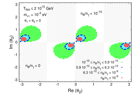
Figure 1: Constraints on the $R$-matrix angle $\theta_{2}$ (in radians) defined in Eq. (10), from the requirement of a successful BAU via thermal leptogenesis (compatible with the constraint on $T_{\mathrm{RH}}$ from Eq. (23)). From out- to inner-most rings, the regions are associated with the following BAU ranges: $n_{\text{B}}/n_{\gamma}\in[10^{-10},\,5.9\times 10^{-10}]$, $n_{\text{B}}/n_{\gamma}\in[5.9\times 10^{-10},\,6.3\times 10^{-10}]$, $n_{\text{B}}/n_{\gamma}\in[6.3\times 10^{-10},\,10^{-9}]$ and $n_{\text{B}}/n_{\gamma}\gtrsim 10^{-9}$.

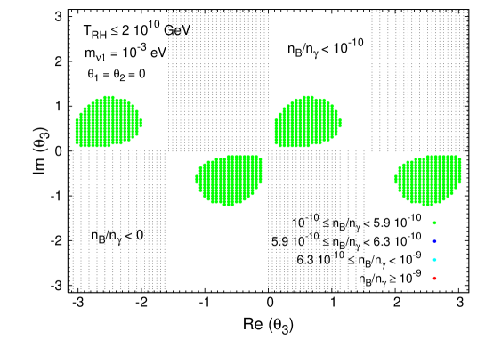
Figure 2: Constraints on the $R$-matrix angle $\theta_{3}$ defined in Eq. (10), from the requirement of successful BAU via thermal leptogenesis with the constraint $T_{\mathrm{RH}}\lesssim 2\,\times\,10^{10}\,\text{GeV}$. Colour code as in Fig. 1 (in this case only the region $n_{\text{B}}/n_{\gamma}\in[10^{-10},\,5.9\times 10^{-10}]$ is present).

Figure 1 illustrates the impact of $\theta_{2}$ (with $\theta_{1}=\theta_{3}=0$) on the estimated BAU. As one can see, the 68% WMAP confidence range of Eq. (28) corresponds to a very narrow ring (represented by the darkest region in Fig. 1) in the Re($\theta_{2}$)-Im($\theta_{2}$) plane. Notice also that values of either Re($\theta_{2}$) or Im($\theta_{2}$) larger than 1.2 radians (mod $\pi$) lead to very small values of the BAU,namely $n_{\text{B}}/n_{\gamma}<10^{-10}$. On the other hand, the analogous study of Fig. 2 shows that with just $\theta_{3}$ ($\theta_{1}=\theta_{2}=0$) one cannot accommodate the WMAP range. Similarly, values of Re($\theta_{3}$) or Im($\theta_{3}$) larger than 1.2 radians (mod $\pi$) also lead to excessively small $n_{\text{B}}/n_{\gamma}$ ($<10^{-10}$). Similar results regarding the constraints on $\theta_{2}$ and $\theta_{3}$ from successfull BAU via leptogenesis have been found in [17] and [19]. We also see from Figs. 1 and 2 that a significant part of the parameter space is excluded since the baryon asymmetry is produced with the wrong sign, $n_{\mathrm{B}}/n_{\gamma}<0$, which contradicts observation.

Regarding $\theta_{1}$, and even though it cannot independently account for a successful BAU, it may have an impact on leptogenesis if $\theta_{2}$ and/or $\theta_{3}$ are non-zero, as can be inferred from Eq. (27).

For the present study of LFV, we adopt a conservative approach, and we only require the estimated baryon-to-photon ratio to be within the range

$$\frac{n_{\mathrm{B}}}{n_{\gamma}}\in\left[10^{-10},10^{-9}\right].$$ (29)

This broad range for $n_{\text{B}}/n_{\gamma}$ reflects the theoretical uncertainties in our estimate which may come, for instance, from flavour effects in the Boltzmann equations [48, 49, 50] and, more generally, from the approximations made in [44] in order to calculate the efficiency factor $\eta$. To accommodate the extended range of Eq. (29), Figs. 1 and 2 suggest that one should take values of $\theta_{2}$ and $\theta_{3}$ not larger than approximately 1 radian (mod $\pi$).

2.4 Implications for charged lepton EDMs

The presence of CP violating phases in the neutrino Yukawa couplings has further implications on low-energy phenomenology. In particular, RGE running will also induce, in addition to the LFV decays, contributions to flavour conserving CP violating observables, as is the case of the charged lepton EDMs. Here, we also analyse the potential constraints on the SUSY seesaw parameter space arising from the present experimental bounds [51] on the EDMs of the electron, muon and tau.

As argued in [24, 25, 52, 53], the dominant contributions to the EDMs arise from the renormalisation of the charged lepton soft-breaking parameters. In particular, the EDMs are strongly sensitive to the non-degeneracy of the heavy neutrinos, and to the several CP violating phases of the model (in our case, the complex $R$-matrix angles). In the present analysis we estimate the relevant contributions to the charged lepton EDMs, taking into account the associated one-loop diagrams (chargino-sneutrino and neutralino-slepton mediated), working in the mass eigenstate basis, and closely following the computation of [54, 55] and [23]. Instead of conducting a detailed survey, we only use the EDMs as a viability constraint, and postpone a more complete study, including all phases, to a forthcoming work. The discussion of other potential CP violating effects, as for instance CP asymmetries in lepton decays, is also postponed to a future study.

3 Results and discussion

In this section we present the numerical results for the LFV branching ratios arising in the SUSY seesaw scenario previously described. In particular, we aim at investigating the dependence of the BRs on the several input parameters, namely on $\theta_{i}$, $m_{N_{i}}$, and $m_{\nu_{1}}$, and how the results would reflect the impact of a potential $\theta_{13}$ measurement. In all cases, we further discuss how the requirement of a viable BAU would affect the allowed parameter range, and in turn the BR predictions.

Regarding the dependence of the BRs on the CMSSM parameters, and instead of scanning over the full ($M_{1/2},\,M_{0},\,A_{0},\,\tan\beta,\,\text{sign}\,\mu$) parameter space, we study specific points, each exhibiting distinct characteristics from the low-energy phenomenology point of view. We specify these parameters by means of the “Snowmass Points and Slopes” (SPS) cases [56] listed in Table 1.

SPS	$M_{1/2}$ (GeV)	$M_{0}$ (GeV)	$A_{0}$ (GeV)	$\tan\beta$	$\mu$
1 a	250	100	-100	10	$>\,0$
1 b	400	200	0	30	$>\,0$
2	300	1450	0	10	$>\,0$
3	400	90	0	10	$>\,0$
4	300	400	0	50	$>\,0$
5	300	150	-1000	5	$>\,0$

Table 1: Values of $M_{1/2}$, $M_{0}$, $A_{0}$, $\tan\beta$, and sign $\mu$ for the SPS points considered in the analysis.

These points are benchmark scenarios for an mSUGRA SUSY breaking mechanism. Points 1a and 1b are “typical” mSUGRA points (with intermediate and large $\tan\beta$, respectively), lying on the so-called bulk of the cosmological region. The focus-point region for the relic abundance is represented by SPS 2, also characterised by a fairly light gaugino spectrum. SPS 3 is directed towards the coannihilation region, accordingly displaying a very small slepton-neutralino mass difference. Finally, SPS 4 and 5 are extreme $\tan\beta$ cases, with very large and small values, respectively. Since the LFV rates are very sensitive to $\tan\beta$, we will also display the BR predictions as a function of this parameter, with $M_{1/2},\,M_{0},\,A_{0}$ and $\text{sign}\,\mu$ as fixed by the SPS points.

To obtain the low-energy parameters of the model (and thus compute the relevant physical masses and couplings), the full RGEs (including relevant terms and equations for the neutrinos and sneutrinos) are firstly run down from $M_{X}$ to $m_{M}$. At the seesaw scale (in particular at $m_{N_{3}}$), we impose the boundary condition of Eq. (9). After the decoupling of the heavy neutrinos and sneutrinos, the new RGEs are then run down from $m_{N_{1}}$ to the EW scale, at which the observables are computed.

The numerical implementation of the above procedure is achieved by means of the public Fortran code SPheno2.2.2 [58]. The value of $M_{X}$ is derived from the unification condition of the $SU(2)$ and $U(1)$ gauge couplings (systematically leading to a value of $M_{X}$ very close to $2\times 10^{16}$ GeV throughout the numerical analysis), while $|\mu|$ is derived from the requirement of obtaining the correct radiative EW symmetry breaking. The code SPheno2.2.2 has been adapted in order to fully incorporate the right-handed neutrino (and sneutrino) sectors, as well as the full lepton flavour structure [18]. The computation of the LFV branching ratios (for all channels) has been implemented into the code with additional subroutines [18]. Likewise, the code has been enlarged with two other subroutines which estimate the value of the BAU, and evaluate the contributions to the charged lepton EDMs.

The input values used regarding the light neutrino masses and the $U_{\text{MNS}}$ matrix elements are

$$\Delta\,m^{2}_{\text{sol}}\,=\,8\,\times 10^{-5}\,\,\text{eV}^{2}\,,\quad\quad\Delta\,m^{2}_{\text{atm}}\,=\,2.5\,\times 10^{-3}\,\,\text{eV}^{2}\,,$$

$$\theta_{12}\,=\,30^{\circ}\,,\quad\theta_{23}\,=\,45^{\circ}\,,\quad\theta_{13}\,\lesssim\,10^{\circ}\,,\quad\quad\delta\,=\,\phi_{1}\,=\,\phi_{2}\,=\,0\,,$$ (30)

which are compatible with present experimental data (see, for instance, the analysis of [59, 60, 61]). As previously mentioned, we do not address the impact of non-vanishing $U_{\text{MNS}}$ phases (Dirac or Majorana) in the LFV branching ratios. The effects of Majorana phases on the BRs have been discussed in Ref. [26].

Regarding charged lepton EDMs, we require compatibility with the current experimental bounds [51]

$$|d_{e}|\,\lesssim(6.9\pm 7.4)\,\times\,10^{-28}\,\,\text{e.cm}\,,\quad|d_{\mu}|\,\lesssim(3.7\pm 3.4)\,\times\,10^{-19}\,\,\text{e.cm}\,,\quad$$

$$\hskip 28.45274pt-2.2\,\times\,10^{-17}\,\lesssim\,d_{\tau}\,\lesssim 4.5\,\times\,10^{-17}\,\,\text{e.cm}\,.$$ (31)

Finally, and before beginning the numerical analysis and discussion of the results, we briefly summarise in Table 2 the present LFV bounds [62, 63, 64, 65, 66], as well as the future planned sensitivities [67, 68, 69, 70], for the several channels under consideration.

LFV process	Present bound	Future sensitivity
BR($\mu\to e\,\gamma$)	$1.2\times 10^{-11}$	$1.3\times 10^{-13}$
BR($\tau\to e\,\gamma$)	$1.1\times 10^{-7}$	$10^{-8}$
BR($\tau\to\mu\,\gamma$)	$6.8\times 10^{-8}$	$10^{-8}$
BR($\mu\to 3\,e$)	$1.0\times 10^{-12}$	$10^{-13}$
BR($\tau\to 3\,e$)	$2.0\times 10^{-7}$	$10^{-8}$
BR($\tau\to 3\,\mu$)	$1.9\times 10^{-7}$	$10^{-8}$

Table 2: Present bounds and future sensitivities for the LFV processes.

3.1 Sensitivity to $\theta_{13}$ in the case $R=\mathbbm{1}$

We begin our study by revisiting the $R=\mathbbm{1}$ case which represents the situation where there are no further neutrino mixings in the Yukawa couplings other than those induced by the $U_{\text{MNS}}$. In this case, the BR($\mu\to e\gamma$) dependence on $\theta_{13}$ was first observed in the context of SUSY GUTs [15]. In Ref. [18], a comprehensive study of all the leptonic decay channels was performed (in a full RGE approach), and it was noticed that $\mu\to e\,\gamma$ and $\mu\to 3\,e$ were the channels that exhibited both a clear sensitivity to $\theta_{13}$ and promising prospects from the point of view of experimental detection. Here, we complete the study of [18], also analysing the other LFV channels. More concretely, we investigate how sensitive to $\theta_{13}$ the BR($l_{j}\to l_{i}\,\gamma$) and BR($l_{j}\to 3\,l_{i}$) are. We also add some comments on the comparison between the full and the LLog approximation results.

In Figs. 3 and 4 we plot the branching ratios of the decays $\mu\to e\,\gamma$, $\mu\to 3\,e$, $\tau\to e\,\gamma$ and $\tau\to 3\,e$, as a function of $\theta_{13}$, which we vary in the range $[0^{\circ},\,10^{\circ}]$. We also display, for comparison, the lines associated with the present experimental bounds and future sensitivities. In each case, we consider as input the six SPS points, and take $\theta_{i}\,=\,0$, so that in this case no BAU is generated and there is no flavour mixing arising from the right-handed neutrino sector. Regarding the neutrino masses, we have assumed $m_{\nu_{1}}\,=\,10^{-5}$ eV, while the masses of the heavy right-handed are set to $m_{N}\,=\,(10^{10},\,10^{11},\,10^{14})$ GeV. In particular we have chosen $m_{N_{1}}$ to avoid the gravitino problem in relation with non-thermal LSP production, as explained in Section 2.3.1. Notice that our choice of $m_{N_{3}}$ leads to large values for the third family Yukawa couplings , specifically $(Y_{\nu})_{33}\approx(Y_{\nu})_{32}\approx 0.3$.

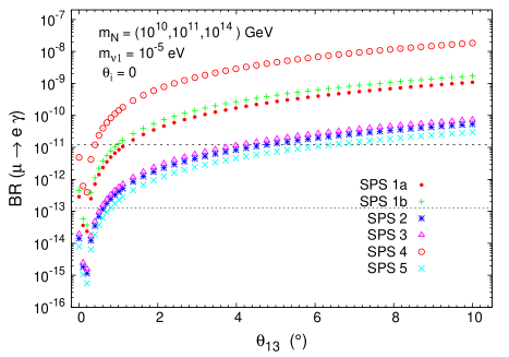
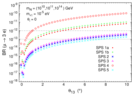
Figure 3: BR($\mu\to e\,\gamma$) and BR($\mu\to 3\,e$) as a function of $\theta_{13}$ (in degrees), for SPS 1a (dots), 1b (crosses), 2 (asterisks), 3 (triangles), 4 (circles) and 5 (times). A dashed (dotted) horizontal line denotes the present experimental bound (future sensitivity).

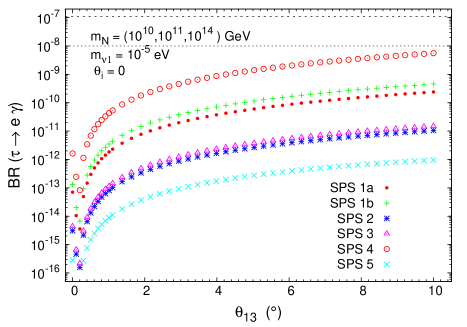
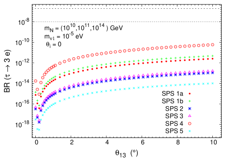
Figure 4: BR($\tau\to e\,\gamma$) and BR($\tau\to 3\,e$) as a function of $\theta_{13}$ (in degrees) for SPS 1a, 1b, 2, 3, 4 and 5. Line and colour codes as in Fig. 3.

The first conclusion to be inferred from Fig. 3 is that, in agreement with [18], the sensitivity to $\theta_{13}$ is clearly manifest in the $\mu\to e\,\gamma$ and $\mu\to 3\,e$ channels. In addition, Fig. 4 shows that BR($\tau\to e\,\gamma$) and BR($\tau\to 3\,e$) also display a strong dependence on $\theta_{13}$. Notice that in these tau decays the BR predictions for the explored $\theta_{13}$ values lie below the present and future experimental sensitivities.

The observed qualitative behaviour with respect to $\theta_{13}$ can be easily understood from Eq. (2.2), which predicts that the dominant contribution proportional to $(L_{33}\,m_{N_{3}}\,m_{\nu_{3}})^{2}$ should grow as $(c_{13}\,s_{13})^{2}$. For small values of $\theta_{13}$ , the “dip” exhibited by the BRs is a consequence of a shift in $\theta_{13}$ arising from RGE running, changing it from $\theta_{13}\equiv\theta_{13}(m_{Z})$ to $\theta_{13}(m_{M})$. Renormalisation induces, in our example, that $\theta_{13}({m_{M}})\approx\theta_{13}({m_{Z}})-0.2^{\circ}$, so that the minimum of the BR is shifted from $\theta_{13}=0^{\circ}$ to $\theta_{13}\approx 0.2^{\circ}$ (which is consistent with analytical estimates [74]). More explicitly, even when starting with a value $\theta_{13}=0^{\circ}$ at the EW scale, RGE running leads to the appearance of a negative value for $\theta_{13}(m_{M})$ (or, equivalently, a non-zero positive $\theta_{13}$ and $\delta=\pi$).

Concerning the $\tau\to\mu\,\gamma$ and $\tau\to 3\,\mu$ channels, the corresponding branching ratios do not exhibit any noticeable dependence on $\theta_{13}$, as expected from the analytical expressions of the LLog approximation. For the case $R=\mathbbm{1}$, and taking for example $\theta_{13}=5^{\circ}$, these BRs are presented in Table 3.

BR	SPS 1a	SPS 1b	SPS 2	SPS 3	SPS 4	SPS 5
$\tau\to\mu\,\gamma$	$4.2\times 10^{-9}$	$7.9\times 10^{-9}$	$1.8\times 10^{-10}$	$2.6\times 10^{-10}$	$9.7\times 10^{-8}$	$1.9\times 10^{-11}$
$\tau\to 3\,\mu$	$9.4\times 10^{-12}$	$1.8\times 10^{-11}$	$4.1\times 10^{-13}$	$5.9\times 10^{-13}$	$2.2\times 10^{-10}$	$4.3\times 10^{-14}$

Table 3: Predictions for the BR($\tau\to\mu\,\gamma$) and BR($\tau\to 3\,\mu$) corresponding to the SPS points. The values of $m_{N_{i}}$ and $m_{\nu_{1}}$ are as specified in Figs. 3 and 4. In each case, the predicted values should be compared with the present bounds (future prospects) BR($\tau\to\mu\,\gamma$) $<$ $6.8\times 10^{-8}$ ($10^{-8}$) and BR($\tau\to 3\,\mu$) $<$ $1.9\times 10^{-7}$ ($10^{-8}$).

The conclusion to be inferred from Figs. 3, 4 and Table 3 is that, for the assumed value of $m_{\nu_{1}}$, and for the chosen seesaw scenario (which is specified by $\theta_{i}$ and $m_{N_{i}}$), the experimental bounds for BR($\tau\to\mu\,\gamma$) already disfavour the CMSSM scenario of SPS 4 (for any value of $\theta_{13}$). From the comparative analysis of the $\theta_{13}$-sensitive channels it is also manifest that $\mu\to e\,\gamma$ and $\mu\to 3\,e$ are the decays whose BRs are within the reach of present experiments, thus potentially allowing to constrain the values of $\theta_{13}$. In fact, BR($\mu\to e\,\gamma$) suggests that SPS 4, 1(a and b), 3, 2 and 5 are disfavoured for values of $\theta_{13}$ larger than approximately $0.5^{\circ}$, $1^{\circ}$, $4^{\circ}$, $5^{\circ}$ and $6^{\circ}$, respectively, while a similar analysis of BR($\mu\to 3\,e$) would exclude $\theta_{13}$ values above $1^{\circ}$, $3^{\circ}$ and $4^{\circ}$ for SPS 4, 1a and 1b, correspondingly. Nevertheless, it is crucial to notice that, as can be seen from Eqs. (2.2, 21), the value of $m_{N_{3}}$ plays a very relevant role. For instance, by lowering $m_{N_{3}}$ from $10^{14}$ GeV to $10^{13}$ GeV one could have compatibility with the experimental bound on BR($\mu\to e\,\gamma$) for $\theta_{13}\lesssim 2^{\circ}$ for all SPS scenarios. Moreover, in this case, even SPS 4 would be in agreement with the experimental bound on BR($\tau\to\mu\,\gamma$).

The relative predictions for each of the SPS points can be easily understood from the BRs dependence on the SUSY spectrum and $\tan\beta$, which is approximately given by Eq. (21). However, it is worth emphasising that although the several approximations leading to Eq. (21) do provide a qualitative understanding of the LFV rates, they are not sufficiently accurate, and do fail in some regions of the CMSSM parameter space. In particular, for the SPS 5 scenario, we have verified that the LLog predictions for the BRs arising from Eq. (2.2) differ from our results by several orders of magnitude. We will return to this discussion at a later stage.

As already mentioned, in the context of SUSY GUTs, the dependence of the BR($\mu\to e\,\gamma$) on $\theta_{13}$ for the same set of SPS points was presented in [15]. Instead of the full computations, the analysis was done using the LLog approximation, and the amount of slepton flavour violation was parameterised by means of mass insertions. In general, and even though a different seesaw scenario was considered, the results are in fair agreement with Fig. 3, the only exception occurring for SPS 5. In fact, while [15] predicts the largest BR($\mu\to e\,\gamma$) for the SPS 5 case, our results of Fig. 3 show that the rates for this point are indeed the smallest ones. As already mentioned, this is due to the failure of the LLog for SPS 5.

Henceforth, and in view of the fact that not only is the decay $\mu\to e\,\gamma$ one of the most sensitive to $\theta_{13}$, but it is also the most promising regarding experimental detection, we will mainly focus our discussion on the analysis of BR($\mu\to e\,\gamma$).

3.2 Implications of a favourable BAU scenario on the sensitivity to $\theta_{13}$

Motivated by the generation of a sufficient amount of CP asymmetry in the decay of the right-handed heavy neutrinos, one has to depart from the $R=\mathbbm{1}$ case, and this will naturally affect the predictions for the several BRs. Nevertheless, it is worth stressing that the hierarchy of the SPS points regarding the relative predictions to the distinct LFV observables is not altered, and we also observe the same ordering as that emerging from Figs. 3, 4 and Table 3, namely BR₄ $>$ BR${}_{\text{1b}}$ $\gtrsim$ BR${}_{\text{1a}}$ $>$ BR₃ $\gtrsim$ BR₂ $>$ BR₅.

As discussed in Section 2.3, the $R$-matrix complex parameters $\theta_{2}$ and $\theta_{3}$ are instrumental in obtaining a value for the baryon asymmetry in agreement with experimental observation, while $\theta_{1}$ plays a comparatively less relevant role. In what follows, we discuss how requiring a favourable BAU scenario would constrain the $\theta_{i}$ ranges, and how this would reflect on the BRs’ sensitivity to $\theta_{13}$.

3.2.1 Influence of $\theta_{2}$

In view of the above, we begin by analysing the dependence of the BR($\mu\to e\,\gamma$) on $\theta_{2}$ and consider two particular values of $\theta_{13}$, $\theta_{13}=0^{\circ}\,,5^{\circ}$. We choose SPS 1a, and motivated from the discussion regarding Fig. 1, take $0\,\lesssim\,|\theta_{2}|\,\lesssim\,\pi/4$, with $\arg\theta_{2}\,=\,\{\pi/8\,,\,\pi/4\,,\,3\pi/8\}$.

In Fig. 5, we display the numerical results, considering $m_{\nu_{1}}\,=\,10^{-5}$ eV and $m_{\nu_{1}}\,=\,10^{-3}$ eV, while for the heavy neutrino masses we take $m_{N}\,=\,(10^{10},\,10^{11},\,10^{14})$ GeV.

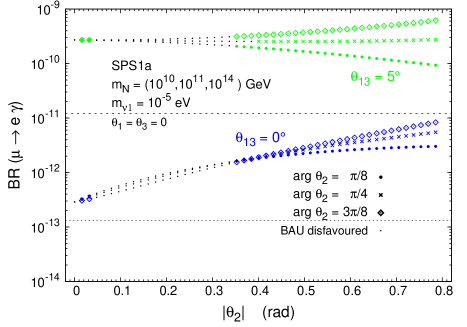
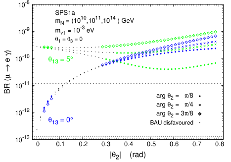
Figure 5: BR($\mu\to e\,\gamma$) as a function of $|\theta_{2}|$, for $\arg\theta_{2}\,=\,\{\pi/8\,,\,\pi/4\,,\,3\pi/8\}$ (dots, times, diamonds, respectively) and $\theta_{13}=0^{\circ}$, 5^∘ (blue/darker, green/lighter lines). We take $m_{\nu_{1}}\,=\,10^{-5}$ ($10^{-3}$) eV, on the left (right) panel. In all cases black dots represent points associated with a disfavoured BAU scenario and a dashed (dotted) horizontal line denotes the present experimental bound (future sensitivity).

There are several important conclusions to be drawn from Fig. 5. Let us first discuss the case $m_{\nu_{1}}\,=\,10^{-5}$ eV. As previously mentioned, one can obtain a baryon asymmetry in the range $10^{-10}$ to $10^{-9}$ for a considerable region of the analysed $|\theta_{2}|$ range. In particular, a deviation from the $R=\mathbbm{1}$ case as small as for instance, $\theta_{2}\,=\,0.05\,e^{\pi/8\,i}$ can account for an amount of BAU close to the WMAP value. A wide region with larger values of $|\theta_{2}|$ ($0.3\lesssim|\theta_{2}|\lesssim 0.8$) can also accommodate a viable baryon asymmetry, as can be seen from Fig. 5. Notice also that there is a clear separation between the predictions of $\theta_{13}=0^{\circ}$ and $\theta_{13}=5^{\circ}$, with the latter well above the present experimental bound. At present, this would imply an experimental impact of $\theta_{13}$, in the sense that the BR predictions become potentially detectable for this non-vanishing $\theta_{13}$ value. With the planned MEG sensitivity [67], both cases would be within experimental reach. However, this statement is strongly dependent on the assumed parameters, in particular $m_{\nu_{1}}$. For instance, a larger value of $m_{\nu_{1}}=10^{-3}$ eV, illustrated on the right panel of Fig. 5, leads to a very distinct situation regarding the sensitivity to $\theta_{13}$. While for smaller values of $|\theta_{2}|$ the branching ratio displays a clear sensitivity to having $\theta_{13}$ equal or different from zero (a separation larger than two orders of magnitude for $|\theta_{2}|\lesssim 0.05$), the effect of $\theta_{13}$ is diluted for increasing values of $|\theta_{2}|$. For $|\theta_{2}|\gtrsim 0.3$ the BR($\mu\to e\,\gamma$) associated with $\theta_{13}\,=\,5^{\circ}$ can be even smaller than for $\theta_{13}\,=\,0^{\circ}$. This implies that in this case, a potential measurement of BR($\mu\to e\,\gamma$) would not be sensitive to $\theta_{13}$.

Moreover, $m_{\nu_{1}}$ also affects the BAU-favoured regions. In general, larger values of $m_{\nu_{1}}$ (still smaller than $10^{-3}$ eV) widen the range of $|\theta_{2}|$ for which a viable BAU can be obtained. This can be understood from the fact that for very small (or zero) $\theta_{2}$ and $\theta_{3}$ (and with fixed $m_{N_{1}}$), $m_{\nu_{1}}$ controls the size of the Yukawa couplings to the lightest right-handed neutrino, $N_{1}$. On the other side, these are the Yukawa couplings governing the washout parameter $\widetilde{m}_{1}$ for thermal leptogenesis, as introduced in Eq. (25). For very small $\theta_{2}$ and $\theta_{3}$, an optimal value $\widetilde{m}_{1}\approx 10^{-3}$ eV can be reached for $m_{\nu_{1}}\approx 10^{-3}$ eV (c.f. Eq. (27)), whereas smaller $m_{\nu_{1}}$ lead to suppressed leptogenesis in this case. For larger values of $\theta_{2}$ and/or $\theta_{3}$, which can be still consistent with leptogenesis, $m_{\nu_{1}}$ becomes less important, since the other light neutrino masses $m_{\nu_{2}}$ and/or $m_{\nu_{3}}$ contribute to $\widetilde{m}_{1}$ as well. In most of the following analysis, we will use $m_{\nu_{1}}\approx 10^{-3}$ eV and enable a successful thermal leptogenesis by introducing a small $R$-matrix rotation angle $\theta_{2}$. In what concerns the sensitivity to $\theta_{13}$ via LFV, this is clearly a conservative choice since, as previously mentioned, lower values of $m_{\nu_{1}}$ (e.g. $m_{\nu_{1}}=10^{-5}$ eV) would lead to a more favourable situation.

Whether or not a BAU-compatible SPS 1a scenario would be disfavoured by current experimental data on BR($\mu\to e\,\gamma$) requires a careful weighting of several aspects. Even though Fig. 5 suggests that for this particular choice of parameters only very small values of $\theta_{2}$ and $\theta_{13}$ would be in agreement with current experimental data, a distinct choice of $m_{N_{3}}$ (e.g. $m_{N_{3}}=10^{13}$ GeV) would lead to a rescaling of the estimated BRs by a factor of approximately $10^{-2}$. Although we do not display the associated plots here, in the latter case nearly the entire $|\theta_{2}|$ range would be in agreement with experimental data (in fact the points which are below the present MEGA bound on Fig. 5 would then lie below the projected MEG sensitivity).

Regarding the other SPS points, which are not shown here, we find BRs for SPS 1b comparable to those of SPS 1a. Smaller ratios are associated with SPS 2, 3 and 5, while larger (more than one order of magnitude) BRs occur for SPS 4.

Let us now consider how the value of $m_{N_{1}}$ affects the amount of BAU, and thus indirectly the branching ratio associated to a given choice of $\theta_{2}$ that accounts for a viable BAU scenario. In Fig. 6 we present the BR($\mu\to e\,\gamma$) as a function of $|\theta_{2}|$ for two distinct heavy neutrino spectra: $m_{N}\,=\,(5\,\times\,10^{9},\,10^{11},\,10^{14})$ GeV and $m_{N}\,=\,(5\,\times\,10^{10},\,10^{11},\,10^{14})$ GeV (values for $m_{N_{1}}$ respectively smaller and larger than what was previously considered). Regarding $\arg\theta_{2}$, we have chosen an example which represents a minimal deviation from the real case, $\arg\theta_{2}\,=\,0.2$, and set $\theta_{1}\,=\theta_{3}\,=0$. We consider SPS 1a, and again show both cases associated with $\theta_{13}\,=\,0^{\circ}\,,5^{\circ}$.

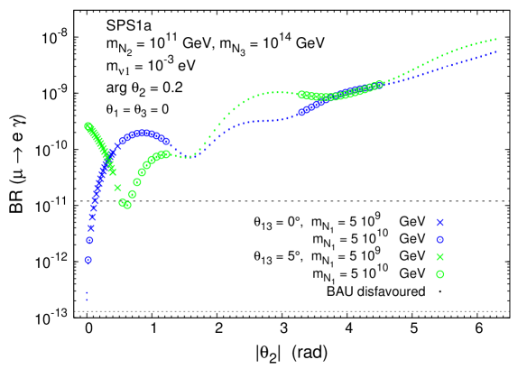
Figure 6: BR($\mu\to e\,\gamma$) as a function of $|\theta_{2}|$, for SPS 1a, with $\arg\theta_{2}\,=\,0.2$. $\theta_{13}\,=\,0^{\circ}\,,5^{\circ}$ (blue/darker, green/lighter lines, respectively), and $m_{N_{1}}=5\,\times\,10^{9}$ GeV, $5\,\times\,10^{10}$ GeV (crosses, circles, respectively). Dots represent points associated with a disfavoured BAU scenario for either $m_{N_{1}}=5\,\times\,10^{9}$ or $5\,\times\,10^{10}$ GeV and a dashed (dotted) horizontal line denotes the present experimental bound (future sensitivity).

From this figure, it can be seen that in the case $m_{N_{1}}=5\,\times\,10^{9}$ GeV, only one BAU-favoured window is opened, for small values of $\theta_{2}$ ($0<\theta_{2}\lesssim\pi/4$). In contrast, for $m_{N_{1}}=5\,\times\,10^{10}$ GeV, a second window opens, corresponding to the $\mod\pi$ periodicity evidenced in Fig. 1 (also some additional points at very small $|\theta_{2}|$ are allowed). The width of the $|\theta_{2}|$ interval for this second window shrinks with decreasing $m_{N_{1}}$. In particular, for $m_{N_{1}}=10^{10}$ GeV (not displayed) this interval becomes extremely small. The latter effect can be understood from the interplay of $\theta_{2}$ and $m_{N_{1}}$ on the relevant BAU parameters of Eq. (27). While $\widetilde{m}_{1}$ is unchanged and as long as $m_{N_{1}}\lesssim T_{\mathrm{RH}}$, the produced baryon asymmetry increases with $m_{N_{1}}$. For a given value of $m_{N_{1}}$, the disappearance of the second window associated with larger values of $|\theta_{2}|$ ($\pi\lesssim|\theta_{2}|\lesssim 3\,\pi/2$), is due to a stronger washout, which leads to values of $n_{\text{B}}/n_{\gamma}$ below the viable BAU range of Eq. (29).

Finally, let us notice that the BAU-favoured ranges of $\theta_{2}$ imply very distinct predictions for both the BRs, and the associated $\theta_{13}$ sensitivity. Even though the BRs arising from the second $\theta_{2}$ window are significantly larger, in this case the sensitivity to $\theta_{13}$ is considerably reduced, as is clearly manifest in Fig. 6. All the previous facts taken into account, we will often rely on the choice $m_{N_{1}}=10^{10}$ GeV and $\theta_{2}\,=\,0.05\,e^{0.2\,i}$ as a means of ensuring a viable BAU scenario via a minimal deviation from the $R=\mathbbm{1}$ case.

3.2.2 Influence of $\theta_{1}$

It has become clear from the previous analysis that a departure from the $R=\mathbbm{1}$ case via non-vanishing values of $\theta_{2}$ can significantly affect the BR sensitivity to $\theta_{13}$. Here we will show that $\theta_{1}$ plays an equally important role on the present discussion. In Figs. 7 and 8 we display the BR($\mu\to e\,\gamma$) as a function of $|\theta_{1}|$, for different values of its argument.

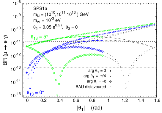
Figure 7: BR($\mu\to e\,\gamma$) as a function of $|\theta_{1}|$, for $\arg\theta_{1}\,=\,\{0\,,\,-\pi/4\,,-\pi\}$ (dots, times, diamonds, respectively) and $\theta_{13}=0^{\circ}\,,5^{\circ}$ (blue/darker, green/lighter lines). BAU is enabled by the choice $\theta_{2}\,=0.05\,e^{0.2\,i}$ ($\theta_{3}\,=0$). In all cases black dots represent points associated with a disfavoured BAU scenario and a dashed(dotted) horizontal line denotes the present experimental bound (future sensitivity).

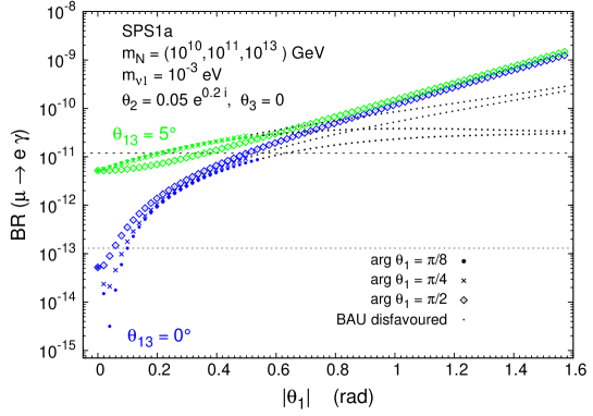
Figure 8: BR($\mu\to e\,\gamma$) as a function of $|\theta_{1}|$, for $\arg\theta_{1}\,=\,\{\pi/8\,,\,\pi/4\,,\pi/2\}$ (dots, times, diamonds, respectively) and $\theta_{13}=0^{\circ}\,,5^{\circ}$ (blue/darker, green/lighter lines). BAU is enabled by the choice $\theta_{2}\,=0.05\,e^{0.2\,i}$ ($\theta_{3}\,=0$). In all cases black dots represent points associated with a disfavoured BAU scenario and a dashed(dotted) horizontal line denotes the present experimental bound (future sensitivity).

As already observed in [18], the effect of departing from the case $R=\mathbbm{1}$ by varying $\theta_{1}$ leads to important additional contributions to the considered LFV decays. Here, we have only presented the case $m_{N_{3}}=10^{13}$ GeV, since for $m_{N_{3}}=10^{14}$ GeV the experimental exclusion line is already crossed for very small values of $\theta_{1}$ ($|\theta_{1}|\approx 0.1$). Opposed to the $\theta_{2}$ case, and as expected from the analytical estimates, there is little dependence of the BR on the choice of the lightest neutrino mass. Considering the other SPS scenarios leads to analogous results, the only difference lying in a global rescaling of the BR($\mu\to e\,\gamma$), and the discussion is similar to that regarding $\theta_{2}$.

In the case of negative arguments, the influence of $\theta_{1}$ is shown in Fig. 7. Notice that in all cases, for extremely small values of $|\theta_{1}|$ ($|\theta_{1}|\lesssim 0.1$), we again recover for $\theta_{13}=5^{\circ}$ BRs which are larger, and clearly distinguishable from the $\theta_{13}=0^{\circ}$ case. In contrast, for a large (negative) $\arg\theta_{1}$, the situation is reversed, and the predictions for BR($\mu\to e\,\gamma$) associated to $\theta_{13}=5^{\circ}$ are actually smaller than for $\theta_{13}=0^{\circ}$. This becomes manifest when $\arg\theta_{1}\lesssim-\pi/2$, a regime for which the BR starts decreasing with increasing $|\theta_{1}|$. For real (and negative) $\theta_{1}$, (i.e. $\arg\theta_{1}=-\pi$) the effect is such that for $\theta_{13}=5^{\circ}$ two local minima of the BR are present (although one disfavoured by BAU), both with an associated value of the BR below the planned MEG sensitivity (for this specific choice of SPS point and seesaw parameters). These “dips” reflect a cancellation between the terms proportional to $m_{\nu_{2}}$ and $m_{\nu_{3}}$ (see Eq. (2.2)), which in fact is also present for $\theta_{13}\approx 0^{\circ}$, albeit only for the second, BAU-disfavoured, $|\theta_{1}|$ value. It is worth pointing out that this apparent accidental cancellation for a specific choice of the $R$-matrix parameters could correspond to the occurrence of texture zeros in the neutrino Yukawa couplings (motivated, for instance, from some flavour symmetry, or arising within specific seesaw models). Although not stable under RGE effects, these zeros effectively translate into very small entries in the Yukawa couplings, which can account for the observed suppression of the BR [18] corresponding to the “dips” in Fig. 7. We would like to remark that, generically, the position and depth of these “dips” depend on the chosen values of all the seesaw parameters.

In Fig. 8 we present a few examples of $\arg\theta_{1}>0$. In this case, the discussion of the BRs and sensitivity to $\theta_{13}$ is very similar to that conducted for small negative arguments. That is, for small $|\theta_{1}|$ values, the predictions for the two $\theta_{13}$ cases are clearly distinguishable. On the other hand, and irrespective of the argument (positive or negative), for sufficiently large $|\theta_{1}|$, the lines corresponding to the cases $\theta_{13}=0^{\circ}$ and 5^∘ eventually meet, and thus for this choice of parameters the sensitivity of the BR to $\theta_{13}$ is lost.

Another relevant aspect to be inferred from Figs. 7 and 8 is how $\theta_{1}$ affects the BAU predictions enabled by $\theta_{2}$. Unlike what occurs for $\theta_{2}$ and $\theta_{3}$, the role of $\theta_{1}$ in accounting for the observed BAU is somewhat more indirect. In particular, and as mentioned in Section 2.3, $\theta_{1}$ essentially deforms the favoured BAU areas in the $\theta_{2}-\theta_{3}$ plane. For instance, and for the chosen BAU-enabling $\theta_{2}$ value in Fig. 7, a real value of $\theta_{1}$ larger than 0.9 leads to an estimated $n_{\text{B}}/n_{\gamma}$ which is no longer within the viable BAU range of Eq. (29). A distinct situation occurs for the cases $\arg\theta_{1}=-\pi/4$ and $\pi/2$, where the entire $|\theta_{1}|$ range successfully accounts for $n_{\text{B}}/n_{\gamma}$ within $[10^{-10},10^{-9}]$.

To conclude this subsection, let us add two further comments. Regarding the influence of $\theta_{3}$ it suffices to mention that although relevant with respect to BAU (see Fig. 2), we have not found a significant BR($\mu\to e\,\gamma$) dependence on the latter parameter. This is a consequence of having the Yukawa couplings to the heaviest right-handed neutrino dominating, since a $\theta_{3}$ $R$-matrix rotation leaves unchanged the couplings $(Y_{\nu})_{i3}$. In this case, the sensitivity to $\theta_{13}$ is very similar to what was found for the $R=\mathbbm{1}$ case. In the remaining analysis we will fix $\theta_{3}=0$.

Concerning the EDMs, which are clearly non-vanishing in the presence of complex $\theta_{i}$, we have numerically checked that for all the explored parameter space, the predicted values for the electron, muon and tau EDMs are well below the experimental bounds given in Eq.(3).

3.3 Dependence on other relevant parameters: $\boldsymbol{m_{N_{3}}}$ and $\boldsymbol{\tan\beta}$

Throughout the discussion regarding the dependence of the branching ratios on the $R$-matrix complex angles, it has often been stressed that the leading contributions to the BRs were those proportional to the mass of the heaviest right-handed neutrino, $m_{N_{3}}$. This is indeed the most relevant parameter. Here, and to briefly summarise the effect of $m_{N_{3}}$, let us present the predictions for BR($\mu\to e\,\gamma$) as a function of the latter mass, while keeping $m_{N_{1}}$ and $m_{N_{2}}$ fixed. We have checked that the BRs do not significantly depend on $m_{N_{1}}$ and $m_{N_{2}}$, apart from one exception for $m_{N_{2}}$, which we will later comment. The results for SPS 1a are displayed in Fig. 9. For completeness, we have included in the upper horizontal axis the associated value of $(Y_{\nu})_{33}$ (with similar values being obtained for $(Y_{\nu})_{32}$).

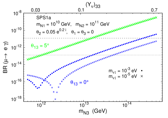
Figure 9: BR($\mu\to e\,\gamma$) as a function of $m_{N_{3}}$ for SPS 1a, with $m_{\nu_{1}}\,=\,10^{-5}$ eV and $m_{\nu_{1}}\,=\,10^{-3}$ eV (times, dots, respectively), and $\theta_{13}=0^{\circ},\,5^{\circ}$ (blue/darker, green/lighter lines). BAU is enabled by the choice $\theta_{2}\,=0.05\,e^{0.2\,i}$ ($\theta_{1}=\theta_{3}=0$). On the upper horizontal axis we display the associated value of $(Y_{\nu})_{33}$. A dashed (dotted) horizontal line denotes the present experimental bound (future sensitivity).

We find from Fig. 9 that the full RGE result grows with $m_{N_{3}}$ in a very similar fashion to that predicted by the LLog approximation, i.e. $m_{N_{3}}^{2}\,\log^{2}m_{N_{3}}$. It is clear that without a predictive theoretical framework for $m_{N_{3}}$ (e.g. GUT models) or indirect experimental evidence for the scale of the seesaw mechanism, there is a large uncertainty regarding the value of $m_{N_{3}}$. Within our chosen scenario of hierarchical heavy neutrinos ($m_{N_{1}}\ll m_{N_{2}}\ll m_{N_{3}}$), assuming that the observed BAU is generated via a mechanism of thermal leptogenesis (with $m_{N_{1}}\gtrsim 10^{9}$ GeV), and given the gauge coupling unification scale ($M_{X}\approx 2\times 10^{16}$ GeV), the natural choice for $m_{N_{3}}$ would lie in the range [$10^{10}$ GeV, $10^{15}$ GeV]. It is obvious from Fig. 9 that such an uncertainty in $m_{N_{3}}$ translates into predictions for the BR ranging over many orders of magnitude. Hence, one can at most extract an upper bound on $m_{N_{3}}$ for the chosen set of input parameters. For instance, in Fig. 9, $m_{N_{3}}\,\gtrsim\,10^{13}\,(10^{14})$ GeV is not allowed by the present experimental bounds on the BR($\mu\to e\,\gamma$) for $\theta_{13}=5^{\circ}\,(0^{\circ})$. Notice that, although the sensitivity to $\theta_{13}$ is clearly displayed in Fig. 9 (with more than two orders of magnitude separation of the $\theta_{13}=0^{\circ}$ and $5^{\circ}$ lines), without additional knowledge of $m_{N_{3}}$ it will be very difficult to disentangle the several $\theta_{13}$ cases. However, this argument can be reversed. This strong dependence on $m_{N_{3}}$ could indeed be used to derive hints on $m_{N_{3}}$ from a potential BR measurement. We will return to this type of considerations in the following section.

It is also worth commenting on the local minima appearing in Fig. 9 for the lines associated with $\theta_{13}=0^{\circ}$. As mentioned before, these “dips” are induced by the effect of the running of $\theta_{13}$, shifting it from zero to a negative value. In the LLog approximation, the “dips” can be understood from Eq. (2.2) as a cancellation between the terms proportional to $m_{N_{3}}\,L_{33}$ and $m_{N_{2}}\,L_{22}$ in the limit $\theta_{13}(m_{M})\to 0^{-}$ (with $\theta_{1}=\theta_{3}=0$). The depth of the minimum is larger for smaller $m_{\nu_{1}}$, as visible in Fig. 9. We have also checked that an analogous effect takes place when one investigates the dependence of BR($\mu\to e\,\gamma$) on $m_{N_{2}}$. It is only in this limit $\theta_{13}(m_{M})\to 0^{-}$, and in the vicinity of the “dip”, that $m_{N_{2}}$ can visibly affect the BRs.

Regarding the other SPS points, with the exception of SPS 3 and 5, the results from the full RGE computation (not displayed here) are also in good agreement with the LLog approximation. The predicted BRs for SPS 3 are found to be larger than those of the LLog by a factor of approximately 3. This divergence is due to the fact that in the LLog approximation the effects of $M_{1/2}$ in the running of the soft-breaking parameters of Eq. (2.2) are not taken into account. Therefore, for low $M_{0}$ and large $M_{1/2}$ (as is the case of SPS 3), there is a significant difference between the results of the full and approximate computations, as previously noted by [78, 79]. Moreover, this difference becomes more evident for low values of $\tan\beta$.

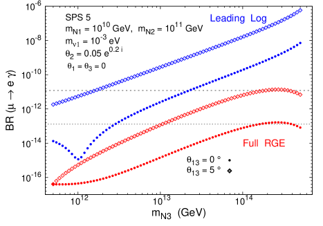
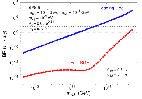
Figure 10: Prediction for BR($\mu\to e\,\gamma$) and BR($\tau\to\mu\,\gamma$) as a function of $m_{N_{3}}$ for SPS 5, using the LLog approximation (upper blue lines) and full RGE (lower red lines). $\theta_{13}=0^{\circ},\,5^{\circ}$ (dots, diamonds, respectively). BAU is enabled by the choice $\theta_{2}\,=0.05\,e^{0.2\,i}$ ($\theta_{1}=\theta_{3}=0$). A dashed (dotted) horizontal line denotes the present experimental bound (future sensitivity).

The divergence of the two computations is more dramatic for SPS 5. This is shown in Fig. 10, where we compare the dependence of the BR($\mu\to e\,\gamma$) and BR($\tau\to\mu\,\gamma$) on $m_{N_{3}}$, as given from the full computation, and in the leading log approximation. The latter approximation over-estimates by more than four orders of magnitude the values of the BR($\mu\to e\,\gamma$). The full RGE and LLog results diverge even more regarding the BR($\tau\to\mu\,\gamma$), with a separation that can be as large as five orders of magnitude. It is also manifest from Fig. 10 that the qualitative behaviour of the full results with respect to $m_{N_{3}}$ is no longer given by $m_{N_{3}}^{2}\,\log^{2}m_{N_{3}}$. The reason for this divergence is associated to the large negative value of the trilinear coupling, $A_{0}$. We considered other large negative values of $A_{0}$, in all cases leading to the same conclusion. Taking large positive $A_{0}$ also leads to an important, albeit not as large, separation (for instance, three orders of magnitude for $A_{0}=1000$ GeV).

Finally, we briefly comment on the BR dependence on $\tan\beta$. As it is well known, the BRs approximately grow as $\tan^{2}\beta$, and therefore this is also a relevant parameter. In Fig. 11, we plot a generalisation of the SPS points 1a and 4 (defined by $M_{0}$, $M_{1/2}$, $A_{0}$ and $\text{sign\,}\mu$) with free $\tan\beta$, and present the sensitivity of the branching ratios to distinct values of $\theta_{13}$.

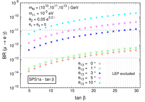
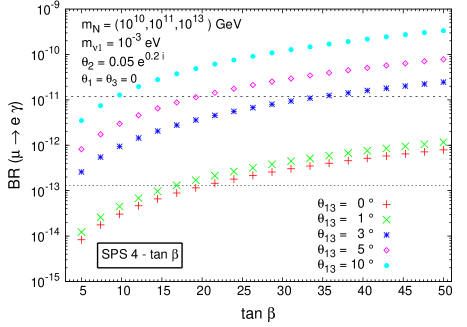
Figure 11: BR($\mu\to e\,\gamma$) as a function of $\tan\beta$, for $m_{N}\,=\,(10^{10},\,10^{11},\,10^{13})$ GeV, for SPS 1a (left) and SPS 4 (right). $\theta_{13}=0^{\circ},1^{\circ},3^{\circ},5^{\circ}$, and $10^{\circ}$ (crosses, times, asterisks, diamonds and dots, respectively). BAU is enabled by the choice $\theta_{2}\,=0.05\,e^{0.2\,i}$ ($\theta_{1}=\theta_{3}=0$). A dashed (dotted) horizontal line denotes the experimental bound (future sensitivity). Vertical shaded regions correspond to regions with spectra excluded by LEP data.

Again, as can be seen in Fig. 11, the sensitivity to $\theta_{13}$ is clearly manifest, in the sense that for a given $\tan\beta$ the predictions for the BRs are very distinct for different $\theta_{13}$ values. However, the $\tan\beta$ dependence is so important that two $\tan\beta$ values, for instance 10 and 20, lead to predictions of the BR that diverge as much as those one obtains from the comparison of $\theta_{13}=3^{\circ}$ and $5^{\circ}$ (for a fixed value of $\tan\beta$). This implies that unless the experimental range for $\tan\beta$ is far more constrained than at present, we cannot conclude about the allowed/disallowed $\theta_{13}$ values from the present $\mu\to e\,\gamma$ bounds. Just like as argued for $m_{N_{3}}$, the strong BR dependence on $\tan\beta$ can be constructively used to further constrain $\tan\beta$ from a potential BR($\mu\to e\,\gamma$) measurement. We will address this topic in the following section.

4 Experimental prospects: hints on SUSY and Seesaw parameters from measuring $\theta_{13}$ and BRs

In the previous section, we analysed how the several free parameters of the SUSY seesaw scenario affect the predictions for the BR($\mu\to e\,\gamma$). We also emphasised how the sensitivity of the latter ratios to $\theta_{13}$ can be altered by the uncertainty introduced from the indetermination of $\theta_{i}$, $\tan\beta$ and, most of all, $m_{N_{3}}$. The question we aim to address in this section is whether a joint measurement of the BRs and $\theta_{13}$ can shed some light on apparently unreachable parameters, like $m_{N_{3}}$.

The expected improvement in the experimental sensitivity to the LFV ratios (see Table 2) support the possibility that a BR be measured in the future, thus providing the first experimental evidence for new physics, even before its discovery at the LHC. The prospects are especially encouraging regarding $\mu\to e\,\gamma$, where the sensitivity will improve by at least two orders of magnitude. Moreover, and given the impressive effort on experimental neutrino physics, a measurement of $\theta_{13}$ will likely also occur in the future [27, 28, 29, 30, 31, 32, 33, 34, 35]. In what follows, let us envisage a future “toy”-like scenario, where we will assume the following hypothesis: (i) measurement of BR($\mu\to e\,\gamma$); (ii) measurement of $\theta_{13}$; (iii) discovery of SUSY at the LHC, with a given spectrum. Furthermore, we assume that BAU is explained via thermal leptogenesis, with a hierarchical heavy-neutrino spectrum.

Under the above conditions, let us conduct the following exercise. First, choosing SPS 1a, $m_{N_{1}}=10^{10}$ GeV, $m_{N_{2}}=10^{11}$ GeV, $m_{\nu_{1}}=10^{-3}$ eV, $\theta_{2}\,=0.05\,e^{0.2\,i}$ (a minimal BAU-enabling deviation from the $R=\mathbbm{1}$ case), and with $\theta_{13}$ set to $1^{\circ}$ ($\pm 0.1^{\circ}$) and to $5^{\circ}$ ($\pm 0.5^{\circ}$), we predict the BRs as a function of $\tan\beta$ and $m_{N_{3}}$. We then plot the contour lines for constant BR values in the $m_{N_{3}}-\tan\beta$ plane. In Fig. 12 we display the corresponding contours for the central values of $1.2\times 10^{-n}$ with $n=10,\dots,15$, allowing for a 10% spread-out around these values. The predicted contours should be compared with the present bound and future sensitivity of $1.2\times 10^{-11}$ [62] and $1.3\times 10^{-13}$ [67], respectively.

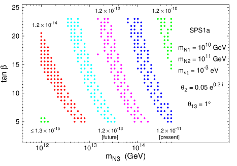
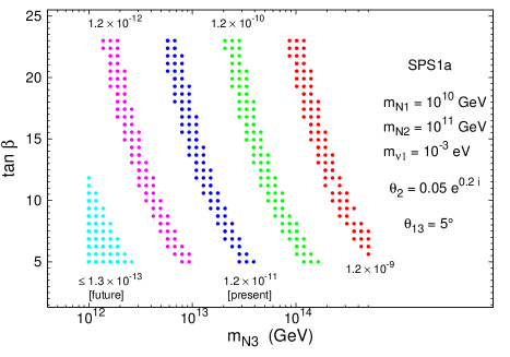
Figure 12: Contours of BR($\mu\to e\,\gamma$)$=(1.2\pm 0.1)\times 10^{-n}$, with $n=10,\dots,15$ in the $m_{N_{3}}-\tan\beta$ plane, for a generalised SPS 1a scenario. We assume $\theta_{13}=1^{\circ}\pm 0.1^{\circ}\,(5^{\circ}\pm 0.5^{\circ})$ on the left (right) panel. BAU is enabled by the choice $\theta_{2}\,=0.05\,e^{0.2\,i}$ ($\theta_{1}=\theta_{3}=0$). The current experimental bound is associated with the darkest (blue) surface, while the future sensitivity is represented by the lightest (cyan) one.

Given a potential SUSY discovery, the implications of a measurement of BR($\mu\to e\,\gamma$) and $\theta_{13}$ are clearly manifest in Fig. 12. From this figure we first learn that, even in the absence of an experimental determination of $\tan\beta$, a potential measurement of BR($\mu\to e\,\gamma$) and $\theta_{13}$ will allow to constrain $m_{N_{3}}$. For example, an hypothetical measurement of BR($\mu\to e\,\gamma$)$\approx 1.2(\pm 0.1)\times 10^{-12}$ would point towards the following allowed ranges of $m_{N_{3}}$:

$$\theta_{13}\,\approx\,1^{\circ}\,\Rightarrow\,\,\,2\,\times\,10^{13}\,\,\text{GeV}\,\lesssim\,m_{N_{3}}\lesssim\,2\,\times\,10^{14}\,\,\text{GeV}\,,$$

$$\theta_{13}\,\approx\,5^{\circ}\,\Rightarrow\,\,\,1.5\,\times\,10^{12}\,\,\text{GeV}\,\lesssim\,m_{N_{3}}\lesssim\,10^{13}\,\,\text{GeV}\,.$$ (32)

Other assumptions for the BRs would equally lead to an order of magnitude interval for the constrained values of $m_{N_{3}}$. If in addition to the s-spectrum, we assume that $\tan\beta$ is experimentally determined, then the intervals for $m_{N_{3}}$ presented in Eq. (4) can be significantly reduced. For instance, assuming that SPS 1a is indeed reconstructed (that is, $\tan\beta=10$), then we would find

$$\theta_{13}\,\approx\,1^{\circ}\,\Rightarrow\,\,\,4\,\times\,10^{13}\,\,\text{GeV}\,\lesssim\,m_{N_{3}}\lesssim\,7\,\times\,10^{13}\,\,\text{GeV}\,,$$

$$\theta_{13}\,\approx\,5^{\circ}\,\Rightarrow\,\,\,3\,\times\,10^{12}\,\,\text{GeV}\,\lesssim\,m_{N_{3}}\lesssim 5\,\times\,10^{12}\,\,\text{GeV}\,.$$ (33)

The hypothetical reconstruction of any other SPS-like scenario would lead to similar one order of magnitude intervals for $m_{N_{3}}$ but with distinct $m_{N_{3}}$ central values. As expected, for the same BR and $\theta_{13}$ measurements, SPS 2, 3 and 5 lead to larger values of $m_{N_{3}}$, the contrary occurring for SPS 1b and 4. This can be seen in Fig. 13, where we present an analogous study to that of Fig. 12, but focusing on SPS 2 and SPS 4, and only considering $\theta_{13}=5^{\circ}\pm 0.5$.

Figure 13: Contours of BR($\mu\to e\,\gamma$)$=(1.2\pm 0.1)\times 10^{-n}$, with $n=10,\dots,15$ in the $m_{N_{3}}-\tan\beta$ plane for a generalised SPS 2 (left) and SPS 4 (right) scenarios. We assume $\theta_{13}=5^{\circ}\pm 0.5^{\circ}$. BAU is enabled by the choice $\theta_{2}\,=0.05\,e^{0.2\,i}$ ($\theta_{1}=\theta_{3}=0$).

Concerning the comparison with current experimental bounds, one can also draw some conclusions regarding the excluded regions of the $m_{N_{3}}$-$\tan\beta$ plane. From both Figs. 12 and  13, for $\theta_{13}=5^{\circ}$, and for the chosen set of input parameters, we infer that in all cases the upper-right regions of the $m_{N_{3}}$-$\tan\beta$ plane are clearly disfavoured. For instance, for SPS 1a, $m_{N_{3}}\gtrsim 10^{14}$ GeV would be excluded for any value of $\tan\beta$. In the case of SPS 2, the exclusion region would be delimited by $\tan\beta\gtrsim 10$ and $m_{N_{3}}\gtrsim 10^{14}$ GeV. The most pronounced exclusion region is for SPS 4, and is given by $\tan\beta\gtrsim 20$, $m_{N_{3}}\gtrsim 10^{13}$ GeV. With the expected future sensitivity, these exclusion regions will be significantly enlarged.

A potential caveat to the previous discussion is the fact that, as seen in Section 3, there is a very important dependence of the BRs on the $R$-matrix parameters $\theta_{i}$. Not only will this have implications on how accurate the indirect estimates of $m_{N_{3}}$ are, but will also affect any judgement regarding the experimental viability of a SUSY seesaw scenario. We recall that, as shown in Section 3, other choices of $\theta_{2}$ (and $\theta_{1}$) can lead to substantially smaller or larger BRs, therefore modifying the exclusion regions of Figs. 12 and  13.

To take into account the strong $R$-matrix dependence, let us conduct in what follows a more comprehensive survey of the parameter space. For SPS 1a, and for distinct choices of the heaviest neutrino mass, we scan over the BAU-enabling $R$-matrix angles (setting $\theta_{3}$ to zero) as

$$0\,\lesssim\,|\theta_{1}|\,\lesssim\,\pi/4\,,\quad\quad-\pi/4\,\lesssim\,\arg\theta_{1}\,\lesssim\,\pi/4\,,$$

$$0\,\lesssim\,|\theta_{2}|\,\lesssim\,\pi/4\,,\quad\quad\quad\,\,\,\,\,\,0\,\lesssim\,\arg\theta_{2}\,\lesssim\,\pi/4\,,$$

$$m_{N_{3}}\,=\,10^{12}\,,\,10^{13}\,,\,10^{14}\,\text{GeV}\,.$$ (34)

Given that, as previously emphasised, $\mu\to e\,\gamma$ is very sensitive to $\theta_{13}$, whereas this is not the case for BR($\tau\to\mu\,\gamma$), and that both BRs display the same approximate behaviour with $m_{N_{3}}$ and $\tan\beta$, we now propose to study the correlation between these two observables. This optimises the impact of a $\theta_{13}$ measurement, since it allows to minimise the uncertainty introduced from not knowing $\tan\beta$ and $m_{N_{3}}$, and at the same time offers a better illustration of the uncertainty associated with the $R$-matrix angles. In this case, the correlation of the BRs with respect to $m_{N_{3}}$ means that, for a fixed set of parameters, varying $m_{N_{3}}$ implies that the predicted point (BR($\tau\to\mu\,\gamma$), BR($\mu\to e\,\gamma$)) moves along a line with approximately constant slope in the BR($\tau\to\mu\,\gamma$)-BR($\mu\to e\,\gamma$) plane. On the other hand, varying $\theta_{13}$ leads to a displacement of the point along the vertical axis. In Fig. 14, we illustrate this correlation for SPS 1a, and for the previously selected $m_{N_{3}}$ and $\theta_{1,2}$ ranges (c.f. Eq. (4)). We consider the following values, $\theta_{13}=1^{\circ}$, $3^{\circ}$, $5^{\circ}$ and $10^{\circ}$, and only include the BR predictions allowing for a favourable BAU. In addition, and as done throughout our analysis, we have verified that all the points in this figure lead to charged lepton EDM predictions which are compatible with present experimental bounds. More specifically, we have obtained values for the EDMs lying in the following ranges (in units of e.cm):

$$10^{-39}\,\lesssim\,|d_{e}|\,\lesssim\,2\times 10^{-35}\,,\,6\times 10^{-37}\,\lesssim\,|d_{\mu}|\,\lesssim\,1.5\times 10^{-32}\,,\,10^{-34}\,\lesssim\,|d_{\tau}|\,\lesssim\,4\times\,10^{-31}\,.$$ (35)

For a fixed value of $m_{N_{3}}$, and for a given value of $\theta_{13}$, the dispersion arising from a $\theta_{1}$ and $\theta_{2}$ variation produces a small area rather than a point in the BR($\tau\to\mu\,\gamma$)-BR($\mu\to e\,\gamma$) plane.

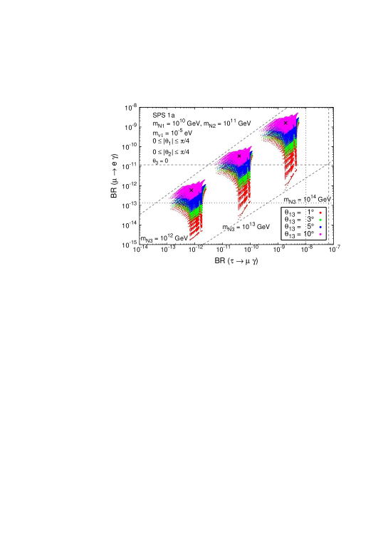
Figure 14: Correlation between BR($\mu\to e\,\gamma$) and BR($\tau\to\mu\,\gamma$) as a function of $m_{N_{3}}$, for SPS 1a. The areas displayed represent the scan over $\theta_{i}$ as given in Eq. (4). From bottom to top, the coloured regions correspond to $\theta_{13}=1^{\circ}$, $3^{\circ}$, $5^{\circ}$ and $10^{\circ}$ (red, green, blue and pink, respectively). Horizontal and vertical dashed (dotted) lines denote the experimental bounds (future sensitivities).

The dispersion along the BR($\tau\to\mu\,\gamma$) axis is of approximately one order of magnitude for all $\theta_{13}$. In contrast, the dispersion along the BR($\mu\to e\,\gamma$) axis increases with decreasing $\theta_{13}$ (in agreement with the findings of Section 3), ranging from an order of magnitude for $\theta_{13}=10^{\circ}$, to over three orders of magnitude for the case of small $\theta_{13}$ ($1^{\circ}$). From Fig. 14 we can also infer that other choices of $m_{N_{3}}$ (for $\theta_{13}\in[1^{\circ},10^{\circ}]$) would lead to BR predictions which would roughly lie within the diagonal lines depicted in the plot. Comparing these predictions for the shaded areas along the expected diagonal “corridor”, with the allowed experimental region, allows to conclude about the impact of a $\theta_{13}$ measurement on the allowed/excluded $m_{N_{3}}$ values.

The most important conclusion from Fig. 14 is that for SPS 1a, and for the parameter space defined in Eq. (4), an hypothetical $\theta_{13}$ measurement larger than $1^{\circ}$, together with the present experimental bound on the BR($\mu\to e\,\gamma$), will have the impact of excluding values of $m_{N_{3}}\gtrsim 10^{14}$ GeV. This lends support to the hints already drawn from Fig. 12. Moreover, with the planned MEG sensitivity, the same $\theta_{13}$ measurement can further constrain $m_{N_{3}}\lesssim 3\times 10^{12}$ GeV. The impact of any other $\theta_{13}$ measurement can be analogously extracted from Fig. 14.

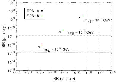
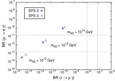
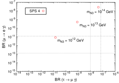
Figure 15: Correlation between BR($\mu\to e\,\gamma$) and BR($\tau\to\mu\,\gamma$) as a function of $m_{N_{3}}$. The points displayed mimic the behaviour of the central $\theta_{13}=10^{\circ}$ marked point in Fig. 14, for SPS points 1a, 1b, 2, 3, 4 and 5. Horizontal and vertical dashed (dotted) lines denote the experimental bounds (future sensitivities).

Similar conclusions can be reached for the other SPS points, as seen in Fig. 15, where we only display the predictions corresponding to the point marked with a cross in the centre of the $\theta_{13}=10^{\circ}$ shaded area of Fig. 14 (taking into account all $\theta_{13}$ values would lead to replications of the shaded areas observed in Fig. 14). Regarding SPS 1b, the discussion is very similar to that of SPS 1a, and the inferred constrains on $m_{N_{3}}$ are almost identical. SPS 2 and SPS 3 offer very close predictions, and when compared to SPS 1a, for the same $\theta_{13}$ measurement, allow to extract slightly weaker bounds on $m_{N_{3}}$. On the other hand, SPS 4 clearly provides the most stringent scenario and a measurement of $\theta_{13}=10^{\circ}$ is only compatible with $m_{N_{3}}\lesssim 10^{12}$ GeV. Notice also that this is the only case where the present experimental bound from BR($\tau\to\mu\,\gamma$) plays a relevant role. SPS 5 provides the weakest bounds on $m_{N_{3}}$ but nevertheless still allows to exclude $m_{N_{3}}\gtrsim 10^{14}$ GeV from a measurement of $\theta_{13}=10^{\circ}$. Finally, it is interesting to notice that the observed correlations for SPS 5 are manifestly different from the other cases, in agreement with the findings of Section 3. In this case, varying $m_{N_{3}}$ leads to predictions of the BR($\mu\to e\,\gamma$) and BR($\tau\to\mu\,\gamma$) which are not linearly correlated, opposed to what would be expected from the LLog approximation.

5 Conclusions

In this work, we have investigated lepton flavour violating muon and tau decays in the CMSSM extended by three right-handed (s)neutrinos, and used a type-I seesaw mechanism to explain the smallness of the neutrino masses. As typical examples of an mSUGRA-like scenario, several SPS SUSY benchmark points were considered. We have parameterised the solutions to the seesaw equation in terms of a complex orthogonal matrix $R$ and of the right-handed neutrino masses, requiring compatibility with low-energy data. We have considered scenarios of hierarchical light and heavy neutrinos. In addition, we imposed consistency with present bounds on charged lepton EDMs and baryogenesis via thermal leptogenesis taking into account constraints on the reheating temperature from non-thermal LSP production by gravitino decay. We have studied in great detail the sensitivity of the BRs to $\theta_{13}$, giving special emphasis to the $\mu\to e\,\gamma$ decay channel.

In a first stage, we have considered the simple case $R=\mathbbm{1}$ where there are no additional neutrino mixings other than those in the $U_{\text{MNS}}$. We have found a very pronounced sensitivity to $\theta_{13}$ in the decay channels $\mu\to e\,\gamma$, $\mu\to 3\,e$, $\tau\to e\,\gamma$ and $\tau\to 3\,e$. Varying $\theta_{13}$ from $0^{\circ}$ to $10^{\circ}$, the branching ratios for the above processes increase by several orders of magnitude. In view of the present experimental bounds and the expected future sensitivity, $\mu\to e\,\gamma$ is by far the most promising channel to study the sensitivity to $\theta_{13}$ in LFV processes. We would like to notice that $\mu\to 3\,e$ may also offer interesting additional information. We have presented the predictions for the branching ratios for various SPS SUSY benchmark points. We further emphasised the importance of a full numerical computation, which we have found to differ significantly from the LLog approximation in some cases.

We have then explored how the sensitivity of BR($\mu\to e\,\gamma$) to $\theta_{13}$ is altered when we take into account the remaining SUSY seesaw parameters. In this sense, we have found that the most relevant parameters are $\theta_{1}$, $\theta_{2}$, $m_{N_{3}}$ and $\tan\beta$ and we have systematically studied their influence on the impact of $\theta_{13}$ on BR($\mu\to e\,\gamma$). We have also noticed that the sensitivity to $\theta_{13}$ improves for lower values of $m_{\nu_{1}}$ ($m_{\nu_{1}}\lesssim 10^{-3}$ eV).

Compared to the special case $R=\mathbbm{1}$, non-vanishing $\theta_{i}$ can have important consequences. In particular, the sensitivity to $\theta_{13}$ is considerably reduced for large values of $|\theta_{1}|$ and $|\theta_{2}|$. However, thermal leptogenesis severely constrains $\theta_{2}$ and $\theta_{3}$ (but not generically $\theta_{1}$). In fact, the requirement of successful thermal leptogenesis with constraints on the reheating temperature from non-thermal LSP production by gravitino decay, suggests a region $|\theta_{2,3}|\lesssim 1$. In these ranges, we have studied the sensitivity of the BR to $\theta_{13}$. Generically, the separation between the BR predictions for distinct $\theta_{13}$ is reduced when we move from $R=\mathbbm{1}$ to $R\neq\mathbbm{1}$, and one could be led to the conclusion that the BR sensitivity to $\theta_{13}$ would be reduced. However, we have also found cases of $R\neq\mathbbm{1}$ where, although this separation is reduced, the BR predictions are now larger (and can be above the experimental bounds) and different $\theta_{13}$ values can be distinguished even more efficiently than in the $R=\mathbbm{1}$ case.

Regarding the right-handed neutrino masses, the most relevant one for the LFV BRs is clearly $m_{N_{3}}$ (with a marginal role being played by $m_{N_{2}}$). Even though $m_{N_{1}}$ does not directly affect the BRs, it nevertheless plays a relevant role with respect to baryogenesis. This, together with the assumption of hierarchical right-handed neutrinos, leads furthermore to an indirect lower bound for $m_{N_{3}}$. For a given choice of $\theta_{13}$, the dependence on $m_{N_{3}}$ is so pronounced that for the investigated range $[10^{11}\,\text{GeV},10^{15}\,\text{GeV}]$, the BRs change by over six orders of magnitude. Thus, and even though the sensitivity to $\theta_{13}$ is clearly manifest (for instance, more than two orders of magnitude separation between the BR predictions of $\theta_{13}=1^{\circ}$ and $5^{\circ}$, for a given value of $\theta_{2}$) without additional knowledge of $m_{N_{3}}$ it will be very difficult to disentangle the several $\theta_{13}$ cases.

In a similar fashion, the sensitivity of the BRs to $\theta_{13}$ can be altered by the uncertainty introduced from the indetermination of $\tan\beta$. The study of the generalised SPS points shows that changing $\tan\beta$ from 5 to 50 translates in BR($\mu\to e\,\gamma$) predictions which differ by two orders of magnitude, so that unless there is an experimental determination of $\tan\beta$, it will also be hard to distinguish the distinct $\theta_{13}$ predictions. Moreover, we have emphasised that this strong dependence on $m_{N_{3}}$ and $\tan\beta$ can be constructively used as a means of extracting information on these parameters from a potential joint measurement of $\theta_{13}$ and BR($\mu\to e\,\gamma$).

Remarkably, within a particular SUSY scenario and scanning over specific $\theta_{1}$ and $\theta_{2}$ BAU-enabling ranges for various values of $\theta_{13}$, the comparison of the theoretical predictions for BR($\mu\to e\,\gamma$) and BR($\tau\to\mu\,\gamma$) with the present experimental bounds allows to set $\theta_{13}$-dependent upper bounds on $m_{N_{3}}$. Together with the indirect lower bound arising from leptogenesis considerations, this clearly provides interesting hints on the value of the seesaw parameter $m_{N_{3}}$. For instance, in the SUSY scenario SPS1a and for values of $\theta_{13}$ in the present experimental allowed range, the present MEGA constraint on BR$(\mu\to e\gamma)$ already sets an upper bound on $m_{N_{3}}$, $m_{N_{3}}\lesssim 10^{13}$ GeV for $\theta_{13}\gtrsim 10^{\circ}$ and $m_{N_{3}}\lesssim 6\times 10^{13}$ GeV for $\theta_{13}\gtrsim 3^{\circ}$, as inferred from Fig. 14. These bounds are even more stringent for the case of SPS4 (see Fig. 15) where the present contraint on BR$(\mu\to e\gamma)$ sets an upper bound of $m_{N_{3}}\lesssim 3\times 10^{12}$ GeV for $\theta_{13}\gtrsim 10^{\circ}$ and $m_{N_{3}}\lesssim 10^{13}$ GeV for $\theta_{13}\gtrsim 3^{\circ}$. With the planned future sensitivities, these bounds would further improve by approximately one order of magnitude.

Ultimately, a joint measurement of the LFV branching ratios, $\theta_{13}$ and the sparticle spectrum would be a powerful tool for shedding some light on otherwise unreachable SUSY seesaw parameters.

References

- [1] B. T. Cleveland et al., Astrophys. J. 496 (1998) 505; W. Hampel et al., Phys. lett. B 447 (1999) 127; Q. R. Ahmad et al. [SNO Collaboration], Phys. Rev. Lett. 87 (2001) 071301 [arXiv:nucl-ex/0106015]; Q. R. Ahmad et al. [SNO Collaboration], Phys. Rev. Lett. 89 (2002) 011302 [arXiv:nucl-ex/0204009]; R. Becker-Szendy et al., Nucl. Phys. Proc. Suppl. 38 (1995) 331; Y. Fukuda et al. [Kamiokande Collaboration], Phys. Lett. B 335 (1994) 237; Y. Ashie et al. [Super-Kamiokande Collaboration], Phys. Rev. Lett. 93 (2004) 101801 [arXiv:hep-ex/0404034]; T. Araki et al. [KamLAND Collaboration], Phys. Rev. Lett. 94 (2005) 081801 [arXiv:hep-ex/0406035]; E. Aliu et al. [K2K Collaboration], Phys. Rev. Lett. 94 (2005) 081802 [arXiv:hep-ex/0411038]; T. Araki et al. [KamLAND Collaboration], Phys. Rev. Lett. 94 (2005) 081801 [arXiv:hep-ex/0406035].
- [2] P. Minkowski, Phys. Lett. B 67 (1977) 421; M. Gell-Mann, P. Ramond and R. Slansky, in Complex Spinors and Unified Theories eds. P. Van. Nieuwenhuizen and D. Z. Freedman, Supergravity (North-Holland, Amsterdam, 1979), p.315 [Print-80-0576 (CERN)]; T. Yanagida, in Proceedings of the Workshop on the Unified Theory and the Baryon Number in the Universe, eds. O. Sawada and A. Sugamoto (KEK, Tsukuba, 1979), p.95; S. L. Glashow, in Quarks and Leptons, eds. M. Lévy et al. (Plenum Press, New York, 1980), p.687; R. N. Mohapatra and G. Senjanović, Phys. Rev. Lett. 44 (1980) 912.
- [3] R. Barbieri, D. V. Nanopolous, G. Morchio and F. Strocchi, Phys. Lett. B 90 (1980) 91; R. E. Marshak and R. N. Mohapatra, Invited talk given at Orbis Scientiae, Coral Gables, Fla., Jan. 14-17, 1980, VPI-HEP-80/02; T. P. Cheng and L. F. Li, Phys. Rev. D 22 (1980) 2860; M. Magg and C. Wetterich, Phys. Lett. B 94 (1980) 61; J. Schechter and J. W. F. Valle, Phys. Rev. D 22 (1980) 2227; R. N. Mohapatra and G. Senjanovic, Phys. Rev. D 23 (1981) 165;
- [4] M. Fukugita and T. Yanagida, Phys. Lett. B 174 (1986) 45.
- [5] F. Borzumati and A. Masiero, Phys. Rev. Lett. 57 (1986) 961.
- [6] J. Hisano, T. Moroi, K. Tobe and M. Yamaguchi, Phys. Rev. D 53 (1996) 2442 [arXiv:hep-ph/9510309].
- [7] J. Hisano, T. Moroi, K. Tobe, M. Yamaguchi and T. Yanagida, Phys. Lett. B 357 (1995) 579 [arXiv:hep-ph/9501407].
- [8] J. Hisano and D. Nomura, Phys. Rev. D 59 (1999) 116005 [arXiv:hep-ph/9810479].
- [9] W. Buchmuller, D. Delepine and F. Vissani, Phys. Lett. B 459 (1999) 171 [arXiv:hep-ph/9904219]
- [10] J. A. Casas and A. Ibarra, Nucl. Phys. B 618 (2001) 171 [arXiv:hep-ph/0103065].
- [11] S. Lavignac, I. Masina and C. A. Savoy, Phys. Lett. B 520 (2001) 269 [arXiv:hep-ph/0106245].
- [12] X. J. Bi and Y. B. Dai, Phys. Rev. D 66 (2002) 076006 [arXiv:hep-ph/0112077]
- [13] J. R. Ellis, J. Hisano, M. Raidal and Y. Shimizu, Phys. Rev. D 66 (2002) 115013 [arXiv:hep-ph/0206110].
- [14] T. Fukuyama, T. Kikuchi and N. Okada, Phys. Rev. D 68 (2003) 033012 [arXiv:hep-ph/0304190].
- [15] A. Masiero, S. K. Vempati and O. Vives, New J. Phys. 6 (2004) 202 [arXiv:hep-ph/0407325].
- [16] T. Fukuyama, A. Ilakovac and T. Kikuchi, arXiv:hep-ph/0506295.
- [17] S. T. Petcov, W. Rodejohann, T. Shindou and Y. Takanishi, Nucl. Phys. B 739 (2006) 208 [arXiv:hep-ph/0510404].
- [18] E. Arganda and M. J. Herrero, Phys. Rev. D 73 (2006) 055003 [arXiv:hep-ph/0510405].
- [19] F. Deppisch, H. Päs, A. Redelbach and R. Rückl, Phys. Rev. D 73 (2006) 033004 [arXiv:hep-ph/0511062].
- [20] L. Calibbi, A. Faccia, A. Masiero and S. K. Vempati, arXiv:hep-ph/0605139.
- [21] For a comprehensive review see for instance, Y. Kuno and Y. Okada, Rev. Mod. Phys. 73 (2001) 151 [arXiv:hep-ph/9909265].
- [22] Y. Okada, K. i. Okumura and Y. Shimizu, Phys. Rev. D 61 (2000) 094001 [arXiv:hep-ph/9906446].
- [23] J. R. Ellis, J. Hisano, S. Lola and M. Raidal, Nucl. Phys. B 621 (2002) 208 [arXiv:hep-ph/0109125].
- [24] J. R. Ellis, J. Hisano, M. Raidal and Y. Shimizu, Phys. Lett. B 528 (2002) 86 [arXiv:hep-ph/0111324].
- [25] J. R. Ellis and M. Raidal, Nucl. Phys. B 643 (2002) 229 [arXiv:hep-ph/0206174].
- [26] S. T. Petcov and T. Shindou, arXiv:hep-ph/0605151.
- [27] E. Ables et al. [MINOS Collaboration], Fermilab-proposal-0875; G. S. Tzanakos [MINOS Collaboration], AIP Conf. Proc. 721 (2004) 179.
- [28] M. Komatsu, P. Migliozzi and F. Terranova, J. Phys. G 29 (2003) 443 [arXiv:hep-ph/0210043].
- [29] P. Migliozzi and F. Terranova, Phys. Lett. B 563 (2003) 73 [arXiv:hep-ph/0302274].
- [30] P. Huber, J. Kopp, M. Lindner, M. Rolinec and W. Winter, JHEP 0605 (2006) 072 [arXiv:hep-ph/0601266].
- [31] Y. Itow et al., arXiv:hep-ex/0106019.
- [32] A. Blondel, A. Cervera-Villanueva, A. Donini, P. Huber, M. Mezzetto and P. Strolin, arXiv:hep-ph/0606111.
- [33] P. Huber, M. Lindner, M. Rolinec and W. Winter, arXiv:hep-ph/0606119.
- [34] J. Burguet-Castell, D. Casper, E. Couce, J. J. Gomez-Cadenas and P. Hernandez, Nucl. Phys. B 725 (2005) 306 [arXiv:hep-ph/0503021].
- [35] J. E. Campagne, M. Maltoni, M. Mezzetto and T. Schwetz, arXiv:hep-ph/0603172.
- [36] Z. Maki, M. Nakagawa and S. Sakata, Prog. Theor. Phys. 28 (1962) 870.
- [37] B. Pontecorvo, Sov. Phys. JETP 6 (1957) 429 [Zh. Eksp. Teor. Fiz. 33 (1957) 549]; Sov. Phys. JETP 7 (1958) 172 [Zh. Eksp. Teor. Fiz. 34 (1957) 247].
- [38] Y. Grossman and H. E. Haber, Phys. Rev. Lett. 78 (1997) 3438 [arXiv:hep-ph/9702421].
- [39] A. Brignole and A. Rossi, Nucl. Phys. B 701 (2004) 3 [arXiv:hep-ph/0404211].
- [40] K. S. Babu and C. Kolda, Phys. Rev. Lett. 89 (2002) 241802 [arXiv:hep-ph/0206310].
- [41] P. Paradisi, JHEP 0602 (2006) 050 [arXiv:hep-ph/0508054].
- [42] For a recent discussion and references see: K. Kohri, T. Moroi and A. Yotsuyanagi, Phys. Rev. D 73 (2006) 123511 [arXiv:hep-ph/0507245].
- [43] D. N. Spergel et al., arXiv:astro-ph/0603449.
- [44] G. F. Giudice, A. Notari, M. Raidal, A. Riotto and A. Strumia, Nucl. Phys. B 685 (2004) 89 [arXiv:hep-ph/0310123]; Additional data and numerical results, private communication.
- [45] W. Buchmuller and M. Plumacher, Int. J. Mod. Phys. A15 (2000) 5047 [arXiv:hep-ph/0007176].
- [46] L. Covi, E. Roulet, and F. Vissani, Phys. Lett. B 384 (1996) 169 [arXiv:hep-ph/9605319].
- [47] S. Davidson and A. Ibarra, Phys. Lett. B 535 (2002) 25 [arXiv:hep-ph/0202239].
- [48] A. Abada, S. Davidson, F. X. Josse-Michaux, M. Losada and A. Riotto, JCAP 0604 (2006) 004 [arXiv:hep-ph/0601083].
- [49] E. Nardi, Y. Nir, E. Roulet and J. Racker, JHEP 0601 (2006) 164 [arXiv:hep-ph/0601084].
- [50] A. Abada, S. Davidson, A. Ibarra, F. X. Josse-Michaux, M. Losada and A. Riotto, arXiv:hep-ph/0605281.
- [51] S. Eidelman et al. [Particle Data Group Collaboration], Phys. Lett. B 592 (2004) 1.
- [52] I. Masina, Nucl. Phys. B 671 (2003) 432 [arXiv:hep-ph/0304299].
- [53] Y. Farzan and M. E. Peskin, Phys. Rev. D 70 (2004) 095001 [arXiv:hep-ph/0405214].
- [54] T. Ibrahim and P. Nath, Phys. Rev. D 57 (1998) 478 [Erratum-ibid. D 58: 019901 (1998); D 60: 079903 (1998); D 60: 119901 (1999)] [arXiv:hep-ph/9708456].
- [55] S. Abel, S. Khalil and O. Lebedev, Nucl. Phys. B 606 (2001) 151 [arXiv:hep-ph/0103320].
- [56] B. C. Allanach et al., in Proc. of the APS/DPF/DPB Summer Study on the Future of Particle Physics (Snowmass 2001) ed. N. Graf, Eur. Phys. J. C 25 (2002) 113 [eConf C010630 (2001) P125] [arXiv:hep-ph/0202233].
- [57] S. Antusch, J. Kersten, M. Lindner and M. Ratz, Phys. Lett. B 538 (2002) 87 [arXiv:hep-ph/0203233].
- [58] W. Porod, Comput. Phys. Commun. 153 (2003) 275 [arXiv:hep-ph/0301101].
- [59] M. C. González-Garcia and C. Peña-Garay, Phys. Rev. D 68 (2003) 093003 [arXiv:hep-ph/0306001].
- [60] M. Maltoni, T. Schwetz, M. A. Tortola and J. W. F. Valle, New J. Phys. 6 (2004) 122 [arXiv:hep-ph/0405172].
- [61] G. L. Fogli, E. Lisi, A. Marrone and A. Palazzo, Prog. Part. Nucl. Phys. 57 (2006) 742 [arXiv:hep-ph/0506083].
- [62] M. L. Brooks et al. [MEGA Collaboration], Phys. Rev. Lett. 83 (1999) 1521 [arXiv:hep-ex/9905013].
- [63] B. Aubert et al. [BABAR Collaboration], Phys. Rev. Lett. 96 (2006) 041801 [arXiv:hep-ex/0508012].
- [64] B. Aubert et al. [BABAR Collaboration], Phys. Rev. Lett. 95 (2005) 041802 [arXiv:hep-ex/0502032].
- [65] U. Bellgardt et al. [SINDRUM Collaboration], Nucl. Phys. B 299 (1988) 1.
- [66] B. Aubert et al. [BABAR Collaboration], Phys. Rev. Lett. 92 (2004) 121801 [arXiv:hep-ex/0312027].
-
[67]
S. Ritt [MEGA Collaboration], on the web page
http://meg.web.psi.ch/docs/talks/sritt/mar06novosibirsk/ritt.ppt. - [68] A. G. Akeroyd et al. [SuperKEKB Physics Working Group], arXiv:hep-ex/0406071.
- [69] T. Iijima, “Overview of Physics at Super B-Factory”, talk given at the 6th Workshop on a Higher Luminosity B Factory, KEK, Tsukuba, Japan, November 2004.
- [70] J. Aysto et al., arXiv:hep-ph/0109217.
- [71] The PRIME working group, “Search for the Conversion Process at an Ultimate Sensitivity of the Order of with PRISM”, unpublished; LOI to J-PARC 50-GeV PS, LOI-25, http://psux1.kek.jp/jhf-np/LOIlist/LOIlist.html
- [72] Y. Kuno, Nucl. Phys. Proc. Suppl. 149 (2005) 376.
- [73] F. Deppisch, H. Pas, A. Redelbach, R. Ruckl and Y. Shimizu, Eur. Phys. J. C 28 (2003) 365 [arXiv:hep-ph/0206122].
- [74] S. Antusch, J. Kersten, M. Lindner and M. Ratz, Nucl. Phys. B 674 (2003) 401 [arXiv:hep-ph/0305273].
- [75] S. F. King, JHEP 0209 (2002) 011 [arXiv:hep-ph/0204360].
- [76] T. Blazek and S. F. King, Nucl. Phys. B 662 (2003) 359 [arXiv:hep-ph/0211368].
- [77] J. I. Illana and M. Masip, Eur. Phys. J. C 35 (2004) 365 [arXiv:hep-ph/0307393].
- [78] S. T. Petcov, S. Profumo, Y. Takanishi and C. E. Yaguna, Nucl. Phys. B 676 (2004) 453 [arXiv:hep-ph/0306195].
- [79] P. H. Chankowski, J. R. Ellis, S. Pokorski, M. Raidal and K. Turzynski, Nucl. Phys. B 690 (2004) 279 [arXiv:hep-ph/0403180].