Diagrammatics of the Dimensionally Reduced Action in $\phi^{4}$ theory

Abstract

We describe the Feynman rules for the construction of the Dimensionally Reduced Action (DRA) for a $\phi^{4}$ field theory, as well as rules for the construction of the connected Green functions and the Dimensionally Reduced Effective Action (DREA), the effective action obtained from the DRA. Two and four-point connected Green functions are calculated to illustrate the application of those rules, and to exhibit the subtraction of UV divergences. As the DRA formalism expands about a background field, instead of the high temperature expansion obtained in the usual dimensional reduced field theory, we derive an expansion that is defined for all range of temperatures. We make a low temperature analysis of the DREA by considering soft modes. In particular, we study the case of near zero mass.

Dimensional reduction Weinberg (1980); Ginsparg (1980); Appelquist and Pisarski (1981); Nadkarni (1983) is a powerful tool to describe thermal field theory for high temperatures, reducing it to a stationary field theory which simplifies the calculations, in particular for the description of relativistic heavy ion collision experiments. It also describes very well the behavior of high temperature semi-classical systems and critical phenomena Zinn-Justin (2000). Nevertheless, expanding around infinite temperature introduces problems such as the appearance of spurious divergences. Another problem is that the validity of the theory is restricted to very high temperature systems, being the low-temperature regime not inaccessible from this point of view.

The dimensionally reduced action (DRA), on the other hand, is defined, and well-behaved, for all ranges of temperature, and is free of the spurious divergences that appear in the dimensionally reduced field theory. It is constructed by incorporating quantum fluctuations in an expansion around a classical field configuration which satisfies the equations of motion and the KMS conditions Kubo (1957); Martin and Schwinger (1959). The DRA was proposed and developed in de Carvalho et al. (2001) in $d$ spatial dimensions for scalar and gauge fields, and studied in de Carvalho and Cavalcanti (2002) for $d=0$, which corresponds to the quantum mechanical case.

The first objective in this article is to find simplified rules for the computation of connected and one-particle irreducible (1PI) diagrams, which are the physical thermal-correlators obtained in perturbation theory. Although the rules we give here are for a $\phi^{4}$ theory, it is easy to generalize for any kind of potential, and for other scalar field theories involving more than one interacting field. The DRA for a fermionic field theory will be pending. The second objective is the construction of the effective action from the reduced action, or the Dimensionally Reduced Effective Action (DREA), and its analysis for soft modes and low temperatures.

This article is organized as follows: In section I we will give a brief description of the DRA and the Feynman rules to construct it; in section II, we will generalize the rules to construct connected diagrams, and exhibit two examples, the self-energy and the four-point connected diagrams at one-loop; finally, in section III, we will construct the DREA, and generalize the rules for the construction of $1PI$ diagrams. Then, an analysis of the effective action for soft modes and low temperatures will be made for the massive case, and for small masses.

I Brief introduction to DRA

Following the construction described in de Carvalho et al. (2001), we will start with the definition of the DRA from the partition function ${\cal Z}=\textrm{Tr}~{}\rho$, with the diagonal density matrix defined as

$$\rho[\phi,\phi]=\oint D\varphi~{}\textrm{e}^{-S[\varphi]}.$$

The integral $\oint$ is to be performed over all fields $\varphi(\tau;\bm{x})$ that satisfy the boundary conditions in the euclidean time $\varphi(0;\bm{x})=\varphi(\beta;\bm{x})=\phi(\bm{x})$ with $\beta=1/T$. The original action $S=S_{F}+S_{I}$ is the Klein-Gordon action in euclidean space, where the free part is defined as

$$S_{F}[\varphi]=\int_{\tau{\bm{x}}}\frac{1}{2}\big{[}(\partial_{\tau}\varphi)^{2}+(\bm{\nabla}\varphi)^{2}+m^{2}\varphi^{2}\big{]}.$$ (1)

Here, we use $\int_{\tau}\equiv\int_{0}^{\beta}d\tau$ and $\int_{\bm{x}}\equiv\int d^{d}x$. Expanding the field $\varphi$ around a background field $\hat{\varphi}$ that satisfies the boundary conditions and the equations of motion for the free theory, we obtain the density matrix $\rho=\exp\{-S_{\textrm{\tiny RED}}\}$, where $S_{\textrm{\tiny RED}}$ is the reduced action, defined as

$$\textrm{e}^{-S_{\textrm{\tiny RED}}[\phi]}=\textrm{e}^{-S_{F}[\hat{\varphi}]}\oint D\eta~{}\textrm{e}^{-S_{F}[\eta]-S_{I}[\hat{\varphi}+\eta]},$$

and where $\varphi=\hat{\varphi}+\eta$. Now, the field integration is performed over all fields $\eta(\tau;\bm{x})$ that satisfy the boundary conditions $\eta(0;\bm{x})=\eta(\beta;\bm{x})=0$. The background field is defined as

$$\hat{\varphi}(\tau;\bm{x})=\int_{\bm{p}}h(\tau;p)\tilde{\phi}(\bm{p})\textrm{e}^{i\bm{p\cdot}\bm{x}},$$

where $\tilde{\phi}(\bm{p})$ is the Fourier transformation of $\phi(\bm{x})$, and

$$h(\tau;p)=\frac{\cosh[\omega_{{p}}(\tau-\beta/2)]}{\cosh(\omega_{p}\beta/2)}.$$ (2)

The integral in Fourier space is defined as $\int_{\bm{p}}\equiv\int\frac{d^{d}p}{(2\pi)^{d}}$, and $\omega_{p}=\sqrt{p^{2}+m^{2}}$. This background field then satisfies the equations of motion and the boundary conditions $\hat{\varphi}(0,\bm{x})=\hat{\varphi}(\beta,\bm{x})=\phi(\bm{x})$.

In the construction and applications of the DRA, there will appear three propagators. The first one is the $\phi$ propagator

$$G_{\phi}(p)=\frac{1}{2\omega_{p}\tanh(\beta\omega_{p}/2)},$$ (3)

which is the inverse of the free action in (1), in momentum space. The second one is the free propagator of the $\eta$ fields

$$G_{\eta}(\tau_{1},\tau_{2};p)=\hskip 156.49014pt$$

$$\theta(\tau_{1}-\tau_{2})\frac{\sinh(\omega_{p}\tau_{2})\sinh[\omega_{p}(\beta-\tau_{1})]}{\omega_{p}\sinh(\beta\omega_{p})}+\tau_{1}\leftrightarrow\tau_{2},$$ (4)

which satisfies the boundary conditions. There is also a third propagator, $G_{th}$, constructed with both propagators $G_{\eta}$ and $G_{\phi}$

$$G_{th}(\tau_{1}-\tau_{2};p)=h(|\tau_{1}-\tau_{2}|;p)G_{\phi}(p)$$

$$\quad\equiv G_{\eta}(\tau_{1},\tau_{2};p)+h(\tau_{1};p)h(\tau_{2};p)G_{\phi}(p).\hskip 28.45274pt$$ (5)

In fact, we will see later that if we sum all the contributions for $\phi$ correlation diagrams calculated with the DRA, the last relation will appear in all internal lines for connected diagrams, and in all loops for 1PI diagrams. This propagator is the Fourier transformation of the usual Matsubara propagator: $G_{th}(\tau;\bm{p})=T\sum_{n}\textrm{e}^{\tau\omega_{n}}(\omega_{n}^{2}+\omega_{\bm{p}}^{2})^{-1}$.

Consider the interaction part of the action as

$$S_{I}[\varphi]=\int_{\tau\bm{x}}\left[\frac{1}{2}\delta_{m}\varphi^{2}+\frac{1}{4!}\lambda_{0}\varphi^{4}\right],$$ (6)

$\lambda_{0}$ being the bare coupling with the counterterm $\delta_{\lambda}=\lambda_{0}-\lambda\sim\lambda^{2}$, and $\delta_{m}$ being the mass counterterm, defined as $\delta_{m}=m_{0}^{2}-m^{2}\sim\lambda_{0}$ $m_{0}$ being the bare mass. We will derive the rules to construct the DRA, and calculate correlation functions for that interaction, but our procedure can be easily generalized to any kind of interaction term described by a polynomial in powers of $\phi$. After integration over the $\eta$ fields, hereafter called thermal ghosts, re-exponentiating and neglecting constant terms independent of the temperature, the dimensional reduced effective action DRA will be then

$$S_{\textrm{\tiny RED}}[\phi]=S_{\textrm{\tiny RED}}[0]+S_{\textrm{\tiny RED}}^{F}[\phi]+S_{\textrm{\tiny RED}}^{I}[\phi],$$

where $S_{\textrm{\tiny RED}}[0]$ is the vaccum contribution, $S_{\textrm{\tiny RED}}^{F}[\phi]=S_{F}[\hat{\varphi}]$ is the quadratic free part, and $S_{\textrm{\tiny RED}}^{I}[\phi]$ the interactive part, defined respectively as

$$S_{\textrm{\tiny RED}}[0] = \frac{1}{2}\ln\det G_{\eta}^{-1}+\Gamma_{\eta c}^{(0)},$$

$$S_{\textrm{\tiny RED}}^{F}[\phi] = \frac{1}{2}\int_{\bm{p}}G_{\phi}(p)^{-1}\tilde{\phi}(-\bm{p})\tilde{\phi}(\bm{p}),$$

$$S_{\textrm{\tiny RED}}^{I}[\phi] = \sum_{n=1}^{\infty}\frac{1}{(2n)!}\int_{\bm{p}_{1}\dots\bm{p}_{2n}}\Gamma_{\eta c}^{(2n)}\tilde{\phi}_{1}\dots\tilde{\phi}_{2n},$$

where $\tilde{\phi}_{i}=\tilde{\phi}(\bm{p}_{i})$, and the terms $\Gamma_{\eta c}^{(2n)}(\bm{p}_{1},\dots,\bm{p}_{n})$ are defined as the effective vertices, expressed diagrammatically in FIG. 1. The effective vertices are the terms resulting from the integration of the $\eta$-field, and the sub-index $\eta c$ denotes that they are constructed through connected $\eta$-diagrams. Then, they can be expressed as a series in powers of the coupling constant

$$\Gamma^{(2n)}_{\eta c}=\sum_{r\geq 1}\Gamma_{\eta c}^{(2n,r)},\quad\mathrm{with}\quad\Gamma_{\eta c}^{(2n,r)}\sim{\lambda_{0}}^{r}$$ (7)

defined as

$$-\Gamma_{\eta c}^{(2n,r)} = \left.\frac{(-1)^{r}}{r!}\frac{\delta^{2n}\langle 0|T_{\eta}S_{I}[\hat{\varphi}+\eta]^{r}|0\rangle_{\eta c}}{\delta\tilde{\phi}(\bm{p}_{1})\dots\delta\tilde{\phi}(\bm{p}_{2n})}\right|_{\phi=0},$$

where the term $\langle 0|T_{\eta}~{}{\cal O}|0\rangle_{\eta c}$ has the time ordering applied only to the $\eta$ fields, considering only connected diagrams. The effective vertices $\Gamma_{\eta c}^{(2n,r)}$ are totally symmetric with respect to the momentum parameter.

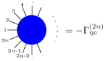
Figure 1: Diagrammatic representation of a DRA effective vertex with $2n$ external $\phi$-lines.

Now, the DRA is expressed in powers of the coupling constant. If we are interested in calculating correlation functions up to order $\lambda^{R}$, we just need to construct the DRA up to such order $S_{\textrm{\tiny RED}}=\sum_{r=0}^{R}{\lambda_{0}}^{r}S_{\textrm{\tiny red}}^{(r)}$. After obtaining the DRA, we can then define the generating functional for the $\phi$ fields, by adding a current source

$${\cal Z}[J]=\int D\phi~{}\textrm{exp}\left\{-S_{\textrm{\tiny RED}}[\phi]+\int_{\bm{x}}J(\bm{x})\phi(\bm{x})\right\}$$ (8)

In the case $J=0$ we obtain the thermodynamic potential: ${\cal Z}[0]=\textrm{exp}\left\{-\beta\Omega\right\}$.

I.1 Feynman rules for the construction of DRA

To obtain the effective vertices of the DRA, let us note first that due to the splitting of the original field into a background field and the quantum fluctuation, $S_{I}[\hat{\varphi}+\eta]$, we will obtain 8 diagrams instead of two, if we consider the interaction in (6): Three vertices with two legs ($-\delta_{m}$), and five vertices with four legs ($-\lambda_{0}$). FIG. 2 shows diagrammatically the different vertices for the construction of the DRA effective vertices.

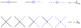
Figure 2: Vertices from the interaction part of the Lagrangian separated in the background field part, containing the $\hat{\varphi}$ field (continuous line), and the fluctuation field part, containing $\eta$ (dashed line).

In terms of Feynman diagrams, the effective vertices are defined as

$$\Gamma^{(2n,r)}_{\eta c}(\bm{p}_{1},\dots,\bm{p}_{2n})=\frac{1}{(2n)!}\Big{[}\gamma_{\eta c}^{(2n,r)}(\bm{p}_{1};\dots;\bm{p}_{2n})$$

$$+\mathrm{all}~{}\bm{p}_{i}\mathrm{-permutations}\Big{]}(2\pi)^{d}\delta({\textstyle\sum\bm{p}_{i})}$$ (9)

where $\gamma^{(2n,r)}_{\eta c}$ are the effective vertex components, the respective Feynman diagrams to order ${\lambda_{0}}^{r}$ computed by integrating over thermal ghosts with $2n$ external $\phi$ legs. In general, we will use semicolons for nonsymmetric dependence on momenta, and commas whenever quantities depend symmetrically. To construct the effective vertices, the Feynman rules are almost the usual ones, except for small modifications.

Rules to calculate the $2n$-points $\sim{\lambda_{0}}^{r}$ effective vertex $-\Gamma_{\eta c}^{(2n,r)}$ in momentum space:

• Draw all the topologically distinct diagrams with $2n$ external $\phi$-lines and connected internal $\eta$-lines formed with $r$ vertices.

• Multiply by $(-\delta_{m})^{c}(-\lambda_{0})^{r-c}/s$ for a diagram constructed with $c$ counterterm vertices, where $s$ is the symmetry factor.

• Multiply by $h(\tau_{i},\bm{p}_{i})$, defined in (2), for every external $\phi_{i}$ line.

• Join the $\eta$ internal lines with the $G_{\eta}$ propagator, defined in (4), imposing momentum conservation.

• Integrate over euclidean time $\tau_{i}$, and over undetermined loop momenta.

• Sum over all external momentum $\bm{p}_{i}$- permutations, and multiply by $(2\pi)^{d}\delta({\textstyle\sum\bm{p}_{i})}/(2n)!$.

A direct consequence of the construction of the effective vertices is the fact that higher-point ($n>2$) effective vertices require more than one vertex of order $\lambda_{0}$ for their construction. Specifically, the tree level $2n$-effective vertex (i.e. without $\eta$-loops) will be of order ${\lambda_{0}}^{n-1}$. This will yield the useful relation

$$\Gamma_{\eta c}^{(2n)}\sim{\lambda_{0}}^{R\geq n-1}.$$ (10)

If we need to make corrections up to order $\lambda^{R}$, we need the DRA up to this order, which includes the tree level component $\phi^{2(R+1)}$.

For example, $\lambda^{2}$ corrections, as we will see in section II.2, will include the term $\sim\Gamma_{\eta c}^{(6,2)}\tilde{\phi}^{6}$, which is negative, and therefore makes the functional integral divergent, as in the case found in de Carvalho and Cavalcanti (2002). Nevertheless, we can always include the next terms: in the present case, if we go to order $\lambda^{3}$, we will include the positive tree-contribution $\sim\Gamma_{\eta c}^{(8,3)}\tilde{\phi}^{8}$, giving the correct convergence of the functional integral.

This procedure can be easily extended to the case of more than one field involved. Particularly, in the case of gauge fields, the DRA can be obtained by using the Feynman gauge, obtaining a tensorial $\eta$-propagator ${G_{\eta}}^{\mu\nu}=\delta^{\mu\nu}G_{\eta}$.

In the next sections, we will exhibit two examples of one-loop diagrams, and how to apply our Feynman rules. Moreover, we will derive more simplified rules to calculate connected and 1PI diagrams.

II Connected diagrams, radiative corrections, and renormalization

We already know the rules to construct the DRA. Depending on the order of the corrections to correlators or observable quantities that we want to obtain, we will construct it up to that order. However, it is not necessary to construct the whole DRA, as we will show. Here, we will present two examples, the most common ones, which are the one-loop correction to the propagator, and the four-point vertex. Such radiative corrections will have ultraviolet divergences that will be canceled by the two counterterms, $\delta_{m}$ and $\delta_{\lambda}$. In fact, those counterterms will be the only terms needed to remove UV divergences to all orders, since the effective theory came from a renormalizable theory.

To calculate connected diagrams, we need the generating functional for the connected green functions $G_{c}[J]=\ln{\cal Z}[J]$ defined from (8). Expressed in terms of the $2n$ connected Green functions, it is defined as

$$G_{c}[J]=-\beta\Omega+\sum_{n=1}\frac{1}{(2n)!}\int_{\bm{p}_{1}\dots\bm{p}_{2n}}G_{c}^{(2n)}\tilde{J}_{1}\dots\tilde{J}_{2n},$$

with $\tilde{J}_{i}\equiv\tilde{J}(\bm{p}_{i})$, the Fourier transformation of $J$. The connected Green functions $G_{c}^{(2n)}(\bm{p}_{1},\dots,\bm{p}_{2n})$ can be expressed in terms of a connected vertex $\Gamma_{c}^{(2n)}$ with $2n$ external legs, which corresponds to the amputated Green function

$$G_{c}^{(2n)}=-\Gamma_{c}^{(2n)}(\bm{p}_{1},\dots,\bm{p}_{2n})G_{\phi}(p_{1})\dots G_{\phi}(p_{2n}),$$

and the thermodynamic potential $\beta\Omega=\Gamma_{c}^{(0)}$. Like the DRA effective vertices, the connected vertices will be totally symmetric, also following the relation in (9), and can be expressed as a series in the renormalized coupling constant $\Gamma_{c}^{(2n)}=\sum_{r\geq 0}\Gamma_{c}^{(2n,r)}$, with $\Gamma_{c}^{(2n,r)}\sim\lambda^{r}$ as in (7). Diagrammatically, $\Gamma_{c}^{(2n,r)}$ corresponds to all the Feynman diagrams of order $\lambda^{r}$ with connected $\eta$ and $\phi$ lines, with the special cases

$$\Gamma_{c}^{(0,0)} = \frac{1}{2}\ln\det G_{\eta}^{-1}+\frac{1}{2}\ln\det G_{\phi}^{-1},$$

$$\Gamma_{c}^{(2,0)} = -G_{\phi}(p_{1})^{-1}(2\pi)^{d}\delta(\bm{p}_{1}+\bm{p}_{2}).$$

II.1 Self energy and mass renormalization.

Although this example was already discussed in de Carvalho et al. (2001), we will explain it here in more detail, in order to explain the notation involved. Starting from the DRA, we need the two-point connected correlator $\langle\tilde{\phi}_{1}\tilde{\phi}_{2}\rangle$ in order to calculate the corrected $\phi$ propagator. To find the self-energy we need only 1PI diagrams,

$$G_{c}^{(2)}(\bm{p}_{1},\bm{p}_{2})=\frac{(2\pi)^{d}\delta(\bm{p}_{1}+\bm{p}_{2})}{G_{\phi}(p_{1})^{-1}+\Sigma(p_{1})},$$

where the self energy is defined as

$$\Sigma(p_{1})(2\pi)^{d}\delta(\bm{p}_{1}+\bm{p}_{2})=\Gamma^{(2)}_{\phi\textrm{\tiny 1PI}}(\bm{p}_{1},\bm{p}_{2}),$$

which defines the one particle irreducible diagrams with respect to the $\phi$ lines. In this case, the connected diagrams of order $\lambda_{0}$ are 1PI: $\Gamma^{(2,1)}_{c}=\Gamma^{(2,1)}_{\phi\textrm{\tiny 1PI}}$. Since we want to compute corrections up to order $\lambda$, and following the rules defined in Section I.1, the respective Feynman diagrams needed to construct the effective vertices are

$$\gamma^{(2,1)}_{{\eta c}-1} = \delta_{m}\int_{\tau}h(\tau,p_{1})h(\tau,p_{2}),$$ (11)

$$\gamma^{(2,1)}_{{\eta c}-2} = \frac{1}{2}\lambda_{0}\int_{\tau\bm{k}}h(\tau,p_{1})h(\tau,p_{2})G_{\eta}(\tau,\tau;k),$$ (12)

$$\gamma^{(4,1)}_{\eta c} = \lambda_{0}\int_{\tau}h(\tau,p_{1})h(\tau,p_{2})h(\tau,p_{3})h(\tau,p_{4}).$$ (13)

They are shown diagrammatically in FIG. 3. Now, we proceed to write the effective vertices as defined in (9). To calculate the connected vertex of order $\lambda$, we resort the usual Feynman rules

$$\Gamma_{c}^{(2,1)} = \Gamma_{\eta c}^{(2,1)}+\frac{1}{2}\int_{\bm{k}}\Gamma_{\eta c}^{(4,1)}(\bm{p}_{1},\bm{p}_{2},\bm{k},-\bm{k})G_{\phi}(k).\hskip 22.76228pt$$ (14)

The sum of the contributions from the diagrams $\gamma_{\eta c-2}^{(2,1)}$ and $\gamma_{\eta c}^{(4,1)}$ gives the relation for the thermal propagator $G_{th}$ defined in (5), yielding the self energy

$$\Sigma(\bm{p}) = \int_{\tau}h(\tau,p)^{2}\left\{\delta_{m}+{\textstyle\frac{1}{2}}\lambda_{0}\int_{\bm{k}}G_{th}(0;k)\right\}.\hskip 14.22636pt$$ (15)

Diagrammatically, the contributions to the self-energy are shown in FIG. 4, where the sum of the thermal ghost line and the $\phi$ line gives the thermal propagator, denoted as a double line, solid and dashed. The thermal propagator in (15) can be written as

$$G_{th}(0;k)=\frac{1}{2\omega_{k}}(2n_{B}(\omega_{k})+1),$$

where $n_{B}(\omega)=(\textrm{e}^{\beta\omega}-1)^{-1}$ is the Bose-Einstein distribution. Then, we can identify the divergent part, which is independent of the temperature. To remove it, we must set

$$\delta_{m}=-\lambda_{0}\int_{\bm{k}}\frac{1}{4\omega_{k}}.$$ (16)

If we want to make higher corrections to the propagator, or one loop corrections to the four-legged vertex, we need to consider the next terms of the DRA.

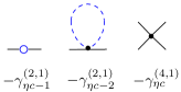
Figure 3: Feynman diagram contributions to the effective vertices at order $\lambda_{0}$

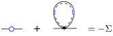
Figure 4: Diagram contribution to the self-energy. The double line, solid and dashed, corresponds to the thermal propagator $G_{th}$.

Setting $\lambda_{0}=\lambda$, and integrating over euclidean time, the corrected propagator will be

$$G(p)^{-1} = G_{\phi}(p)^{-1}+\Sigma(p)$$

$$= 2\omega_{p}\tanh(\omega_{p}\beta/2)$$

$$+\lambda\int_{\bm{k}}\frac{n_{B}(\omega_{k})}{2\omega_{k}}\frac{\beta\omega_{p}+\sinh(\beta\omega_{p})}{2\omega_{p}\cosh(\beta\omega_{p}/2)^{2}}$$

$$= 2\omega\tanh(\omega\beta/2)+{\cal O}(\lambda^{2}),$$

where $\omega^{2}=p^{2}+m_{D}^{2}$ includes the Debye mass defined as $G^{-1}(p^{2}=-m_{D}^{2})=0$. In the present case, it corresponds to

$$m_{D}^{2}=m^{2}+\lambda\int_{\bm{k}}\frac{n_{B}(\omega_{k})}{2\omega_{k}},$$

which is the well known result for the usual one-loop thermal mass calculated with the real or imaginary time formalism.

II.2 Four-point vertex correction and coupling constant renormalization

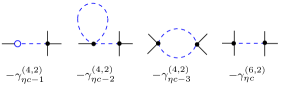
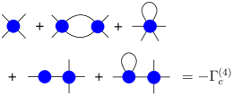
Figure 5: four and six leg contributions to the effective vertices of order ${\lambda_{0}}^{2}$

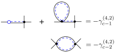
Figure 6: Relevant diagrams for the four-point connected vertex

Figure 7: Contributions to the connected vertex of order $\lambda^{2}$

For the four-point connected vertex, we need the DRA up to order $\lambda^{2}$. Yet, it is not necessary to calculate all the effective vertices. Apart from the order $\lambda_{0}$ contributions already calculated in the previous example, we need the next contributions to the four-point effective vertex, and the first contribution to the six-point effective vertex, which are both of order ${\lambda_{0}}^{2}$. Their respective Feynman diagrams are shown in FIG. 7. Having obtained the effective vertices, we proceed to calculate the four-point connected vertices. The relevant Feynman diagrams are shown in 7, and give as a result

$$-\Gamma^{(4)}_{c} = (2\pi)^{d}\delta({\textstyle\sum\bm{p}_{i})}\Bigg{\{}\gamma_{c}^{(2,1)}(\bm{p}_{1},\bm{p}_{2},\bm{p}_{3},\bm{p}_{4})$$

$$+\frac{1}{4}\big{[}\gamma^{(4,2)}_{c-1}(\bm{p}_{1};\bm{p}_{2},\bm{p}_{3},\bm{p}_{4})+\bm{p}_{1}\leftrightarrow\{\bm{p}_{2},\bm{p}_{3},\bm{p}_{4}\}\big{]}$$

$$+\frac{1}{3}\big{[}\gamma^{(4,2)}_{c-2}(\bm{p}_{1},\bm{p}_{2};\bm{p}_{3},\bm{p}_{4})+\bm{p}_{2}\leftrightarrow\{\bm{p}_{3},\bm{p}_{4}\}\big{]}\Bigg{\}}$$

where $\gamma_{c}^{(4,1)}=\gamma_{\eta c}^{(4,1)}$, described in (13), and $\gamma_{c-1}^{(4,2)}$ and $\gamma_{c-2}^{(4,2)}$ are the the combination of the equivalent terms from the effective vertices contracted with $\phi$ lines described in FIG. 7. Again, the combination of the $\eta$ and $\phi$ propagators gives the thermal propagator $G_{th}$ in all the internal lines. In fact, this will be a general rule in the construction of the connected propagators.

Let us examine first the diagram $\gamma_{c-1}^{(4,2)}$. It is formed by two diagrams involving a closed loop and a counterterm. The ultraviolet divergences are then simply removed by using the value of the counterterm $\delta_{m}$ given in (16). The result is

$$\gamma^{(4,2)}_{c-1}(\bm{p}_{1};\bm{p}_{2},\bm{p}_{3},\bm{p}_{4})=\hskip 113.81102pt$$

$$\quad-2{\lambda_{0}}^{2}\int_{\tau_{1}\tau_{2}}h(\tau_{1},p_{1})h(\tau_{2},p_{2})h(\tau_{2},p_{3})h(\tau_{2},p_{4})$$

$$G_{th}(\tau_{1}-\tau_{2};p_{1})\int_{\bm{k}}\frac{n_{B}(\omega_{k})}{\omega_{k}}.$$ (17)

To find the divergent term in the diagram $\gamma_{c-2}^{(4,2)}$ is not as simple as in the previous case. As one can see, it involves an external momentum dependent loop:

$$\gamma^{(4,2)}_{c-2}(\bm{p}_{1}\bm{p}_{2};\bm{p}_{3},\bm{p}_{4})=\hskip 116.65646pt$$

$$-\frac{3}{2}{\lambda_{0}}^{2}\int_{\tau_{1}\tau_{2}}h(\tau_{1},p_{1})h(\tau_{1},p_{2})h(\tau_{2},p_{3})h(\tau_{2},p_{4})\hskip 2.84544pt$$

$$\int_{\bm{k}}G_{th}(\tau_{1}-\tau_{2};k)G_{th}(\tau_{1}-\tau_{2};|\bm{p}_{1}+\bm{p}_{2}-\bm{k}|).$$ (18)

To identify the divergence, first we need to perform the euclidean time integration. Since the counterterm is momentum independent, we just consider $\bm{p}_{i}=0$

$$\gamma^{(4,2)}_{c}(0) = -{\lambda_{0}}^{2}\int_{\bm{k}}\left\{F(k)+\frac{6\beta m+8\sinh(\beta m)+\sinh(2\beta m)}{16m\cosh(\beta m/2)^{4}}\frac{3}{32{\omega_{k}}^{3}}[2n_{B}(\omega_{k})+1]\right\},$$ (19)

with

$$F(k) = \frac{3~{}\mathrm{sech}(m\beta/2)^{4}}{16m^{2}{\omega_{k}}^{2}}\Bigg{[}\frac{m^{4}}{k^{4}}\left(\frac{\sinh(\beta m)^{2}\cosh(\beta\omega_{k})}{\sinh(\beta\omega_{k}/2)^{2}}-\frac{m}{\omega_{k}}\frac{\sinh(2\beta m)}{\tanh(\beta\omega_{k}/2)}\right)$$

$$\hskip 71.13188pt+\frac{m^{3}}{2\omega_{k}k^{2}}\frac{\beta m-\sinh(2\beta m)}{2\tanh(\beta\omega_{k}/2)}+\left(\frac{\beta m+\sinh(\beta m)}{\sinh(\beta\omega_{k}/2)}\right)^{2}\Bigg{]}.$$

The function $F(k)$ is analytic in the real axis, and its integral is finite for all temperatures. The only divergent term in equation (19) is $\int_{\bm{k}}\omega^{-3}$, in the case of $d=3$. Considering the fact that

$$\int_{\tau}h(\tau,p)^{4}=\frac{6\beta\omega_{p}+8\sinh(\beta\omega_{p})+\sinh(2\beta\omega_{p})}{16\omega_{p}\cosh(\beta\omega_{p}/2)^{4}},$$

we can see that the divergent term is proportional to $\gamma^{(4,1)}(0)$. Then, setting $\lambda_{0}=\lambda+\delta_{\lambda}$, with

$$\delta_{\lambda}=\lambda^{2}\frac{3}{32}\int_{\bm{k}}\frac{1}{\omega_{k}^{3}},$$

we remove the divergence. We can now replace ${\lambda_{0}}^{2}=\lambda^{2}+{\cal O}(\lambda^{3})$ in all the expressions.

Note that in the case of $d\leq 2$ there are no divergent term since the theory is super-renormalizable. However, we will remove this term as a general prescription for any dimension.

There are no more counterterms. All the other divergences will be cancelled with $\delta_{m}$ and $\delta_{\lambda}$, or will be divergences of higher order that can be canceled by re-defining the counterterm with higher order terms.

II.3 Feynman rules for connected diagrams

We can see in the last two examples that the thermal propagator is present in all internal connected vertices. In fact, this will be a general rule, and to obtain connected Green functions it is not necessary to calculate the effective vertices of the DRA. Then, we just need two vertices to describe the different Feynman diagrams: the four-point ($-\lambda_{0}$), and the two-point ($-\delta_{m}$).

Rules to calculate the $2n$-points $\sim{\lambda_{0}}^{r}$ connected vertex $-\Gamma_{c}^{(2n,r)}$ in momentum space:

• Draw all the topologically distinct connected diagrams with $2n$ external lines formed with $r$ vertices.

• Multiply by $(-\delta_{m})^{c}(-\lambda_{0})^{r-c}/s$ for a diagram constructed with $c$ counterterm vertices, where $s$ is the symmetry factor.

• Multiply by $h(\tau_{i},\bm{p}_{i})$, defined in (2), for every external $\phi_{i}$ line.

• Join the internal lines with the $G_{th}$ propagator, defined in (5), imposing momentum conservation.

• Integrate over euclidean time $\tau_{i}$, and over undetermined loop momenta.

• Sum over all external momentum $\bm{p}_{i}$- permutations and multiply by $(2\pi)^{d}\delta({\textstyle\sum\bm{p}_{i})}/(2n)!$.

III The Dimensionally Reduced Effective Action

We will construct the DREA using the standard method to obtain an effective action (see for example Amit (1984)) from the generating functional in equation (8)

$$a^{-1}\Gamma[\Phi]=-G_{c}[J]+\int_{\bm{x}}J(\bm{x})\Phi(\bm{x}),$$ (20)

where $\Phi=\langle\phi\rangle_{J,T}$, and $a$ is a small parameter ($a=\hbar$ in the semiclassical approximation). Now, let us redefine the fields, and scale the original action as

$$\phi=\Phi+\sqrt{a}\phi^{\prime},\quad\eta=\sqrt{a}\eta^{\prime},\quad S[\varphi]\rightarrow a^{-1}S[\varphi].$$

We will define $J=J_{c}+\sqrt{a}~{}\delta_{J}$, where $\delta_{J}$ will be a counterterm which will remove tadpole diagrams, and $J_{c}$ is related with the classical equation of motion through $\delta S_{\textrm{\tiny RED}}[\Phi]/\delta\Phi=J_{c}$. With these assumptions, the DREA will be

$$\Gamma[\Phi]=S_{\textrm{\tiny RED}}[\Phi]-a\ln\int D\phi^{\prime}\mathrm{e}^{-S_{\textrm{\tiny RED}}^{F}[\phi^{\prime}]-\bar{S}[\phi^{\prime},\Phi]-\int_{\bm{x}}\delta_{J}\phi^{\prime}},$$

with

$$\bar{S}[\phi^{\prime},\Phi] = \sum_{n,r=1}^{\infty}\sum_{m=2}^{2n}\frac{a^{m/2-1}}{(2n-m)!~{}m!}\int_{\bm{p}_{1}\dots\bm{p}_{2n}}$$ (21)

$$\Gamma_{\eta c}^{(2n,r)}\tilde{\Phi}_{2n-m+1}\dots\tilde{\Phi}_{2n}~{}\tilde{\phi}^{\prime}_{1}\dots\tilde{\phi}^{\prime}_{m}.$$

Now, we integrate over $\phi^{\prime}$ using $G_{\phi}$ as the propagator. The resulting series will involve N-particle irreducible diagrams. If we re-exponentiate again, the particle reducible diagrams will give rise to tadpoles that will be cancelled by the counterterm $\delta_{J}$. So, the effective action will be

$$\Gamma[\Phi] = a\frac{1}{2}\ln\det G_{\phi}^{-1}+S_{\textrm{\tiny RED}}[\Phi]$$ (22)

$$-a\sum_{s=1}^{\infty}\frac{(-1)^{s}}{s!}\langle 0|S[\phi^{\prime},\Phi]^{s}|0\rangle_{\phi\textrm{\tiny 1PI}}.$$

Reorganizing in powers of the classical $\Phi$ field, the DREA will be

$$\Gamma[\Phi]=\sum_{n=0}\frac{1}{(2n)!}\int_{\bm{p}_{1}\dots\bm{p}_{2n}}\Gamma^{(2n)}\tilde{\Phi}_{1}\dots\tilde{\Phi}_{2n}.$$

The vertices can be expressed in terms of number of loops

$$\Gamma^{(2n)}=\sum_{l\geq 0}\Gamma^{(2n,l)},\quad\mbox{ with}\quad\Gamma^{(2n,l)}\sim\lambda^{n-1}(\lambda a)^{l},$$ (23)

where $l$ denotes the total number of loops, $\eta$ and $\phi$, with the special cases

$$\Gamma^{(0,0)} = 0$$

$$\Gamma^{(0,1)} = \frac{a}{2}(\ln\det G_{\phi}^{-1}+\ln\det G_{\eta}^{-1})$$

$$\Gamma^{(2,0)} = G_{\phi}(\bm{p}_{1})^{-1}(2\pi)^{d}\delta(\bm{p}_{1}+\bm{p}_{2}).$$

To derive equation (23), let us see first how the $a$ parameter changes the effective vertex $\Gamma^{(2n,r)}_{\eta c}$ which involves $r$-vetices, $2n$ external $\phi$ legs, and $I_{\eta}$ internal $\eta^{\prime}$ lines. Since the internal lines involve a pair of $\eta^{\prime}$ fields they will include a term $a^{I_{\eta}}$, a power of $a^{-r}$ due to scaling of $S_{I}$, and one $a$ to get the common scaling factor in the full action. This mean that $\Gamma^{(2n,r)}_{\eta c}\sim{\lambda_{0}}^{r}a^{I_{\eta}-r+1}$. Using the well-known relation

$$L=I-V+1,$$ (24)

for diagrams with $L$-loops, $V$-vertices and $I$-internal lines, we find then that $\Gamma^{(2n,r)}_{\eta c}\sim{\lambda_{0}}^{r}a^{l_{\eta}}$.

We would now like to express the $r$ parameter in terms of the number of $\eta^{\prime}$-loops and external legs. Let us forget for a moment the diagrams which include the counterterm $\delta_{m}$. Since the vertex contains four legs, the sum of the total legs ($\eta^{\prime}$ and $\phi$) will be $4r$, then we obtain the relation $4r=2n+2I_{\eta}$. Together with relation (24) we find that $r=l_{\eta}+n-1$. In the case of vertices with the counterterm $\delta_{m}$, they are equivalent to a four-leg vertex with two legs joined by an internal line. Then $\delta_{m}\sim\lambda_{0}a$. The same will be done for the coupling constant where $\delta_{\lambda}\sim\lambda^{2}a$. The contribution to the effective action $S_{\textrm{\tiny RED}}[\phi]$ in (22) then will include the effective vertices expressed in terms of number of $\eta$-loops

$$\Gamma_{\eta c}^{(2n,r)}=\Gamma_{\eta c}^{(2n,n-1+l_{\eta})}\sim{\lambda_{0}}^{n-1}(\lambda_{0}a)^{l_{\eta}}$$ (25)

To find the other contributions from the integration of the $\phi^{\prime}$ fields, let us consider a general $\phi$-1PI diagram $\gamma_{s}^{(2n,l)}$, constructed with $s$ vertices. From (21) and (22) we have that $\gamma_{s}^{(2n,l)}\sim a\prod_{i=1}^{s}a^{m_{i}/2-1}\Gamma_{\eta c}^{(2n_{i},r_{i})}$, where the sum of all external $\Phi$-legs and internal $\phi$-lines gives respectively $\sum_{i=1}^{s}(2n_{i}-m_{i})=2n$ and $\sum_{i=1}^{s}2m_{i}=I_{\phi}$ (the total number of $\phi^{\prime}$ internal lines). With this, and equations (24) and (25), we obtain that $\gamma_{s}^{(2n,l)}\sim{\lambda_{0}}^{n-1}(\lambda_{0}a)^{l_{\phi}+l_{\eta}}$ where $l_{\phi}+l_{\eta}=l$. Now, if we sum all the diagrams with $2n$ $\Phi$-legs and $l$-loops, and renormalize the mass and the counterterms, we obtain (23).

The DREA will then be an infinite series in powers of the fields, and in the small parameter $a\lambda$ raised to the number of loops. All powers of the fields will be accompanied by a coupling constant $\gamma^{(2n)}\sim\lambda^{n-1}\Phi^{2n}$, independently of the number of loops. Then, if $\Lambda$ defines the scale of validity of the theory, the condition for convergence of the series is that $\underline{\Phi}^{2}<\underline{\lambda}^{-1}$, where the underline stands for scaling with $\Lambda$. So as $\underline{\lambda}\ll 1$, the range of validity of the field for the convergence of the series is wide but always finite.

III.1 Feynman rules for the DREA vertices

Differently from the case of connected diagrams, the thermal propagator will appear in all closed loops in the effective action. To illustrate it, we show one-loop corrections to the two and four-point vertices of the effective action. Hereafter, we turn back to natural units ($a=1$).

In the case of two-point vertices, the one-loop correction is the self-energy calculated in section II.1, where the effective action vertex is the inverse of the connected Green function $\Gamma^{(2)}(\bm{p}_{1},\bm{p}_{2})=G_{c}^{(2)-1}(\bm{p}_{1},\bm{p}_{2})$.

The correction to the four-point vertex is more illustrative. In FIG. 7, the last two diagrams are two-particle reducible with respect to the $\phi$ lines. The four-point vertex of the effective action then will include only the first three diagrams at one loop. The result will change only the diagrams described by $\gamma_{c-1}^{(4,2)}$, illustrated in FIG.  7 and expressed in equation (17) by cutting the internal $\phi$-line that joins the two DRA effective vertices, as can be seen in FIG. 8. This gives as a result the replacement of the propagator $G_{th}(\tau_{1}-\tau_{2};p_{1})$ by $G_{\eta}(\tau_{1},\tau_{2};p_{1})$ in equation (17). So, as in the case of connected diagrams, the DREA vertices will be constructed by considering only two vertices, $-\delta_{m}$ and $-\lambda_{0}$.

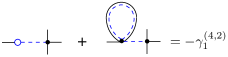
Figure 8: One of the contributions to the four-point vertex of the effective action.

Rules to calculate the $2n$-points and $l$-loops connected vertex $-\Gamma^{(2n,l)}$ in momentum space:

• Construct all the possible topologically distinct $l$-loops connected diagrams with $2n$ external lines.

• Multiply by $(-\delta_{m})^{c}(-\lambda_{0})^{r-c}$ for a diagram constructed with $c$ counterterm vertices, and divide by the symmetry factor.

• Multiply by $h(\tau_{i},\bm{p}_{i})$, defined in (2), for every external $\phi_{i}$ line.

• Join the internal closed loops with the $G_{th}$ propagator, defined in (5), imposing momentum conservation.

• Join the internal, non-loop lines with the $G_{\eta}$ propagator, defined in (4).

• Integrate over euclidean time $\tau_{i}$.

• Integrate over undetermined loop momenta.

• Sum over all external momentum $\bm{p}_{i}$- permutations, and multiply by $(2\pi)^{d}\delta({\textstyle\sum\bm{p}_{i})}/(2n)!$.

III.2 Soft modes in DREA

The main goal of the DRA and DREA is to obtain a reduced theory valid for all ranges of temperature, in particular low temperatures, so this is the main sector we would like to study. In general, the macroscopic information obtained from microscopic systems is encoded in their long range behavior. Then, as we are interested in long distance behavior, we need mainly to extract low-momentum macroscopic parameters, considering only soft modes. In the DREA, soft modes imply the momentum expansion of the $\gamma$ terms,

$$\gamma^{(2n)}(\bm{p}_{i})\approx\gamma^{(2n)}(0),\quad\mathrm{for}\quad n>1,$$

and

$$\gamma^{(2)}(p)\approx\gamma^{(2)}(0)+\frac{\partial\gamma^{(2)}}{\partial p^{2}}(0)p^{2}.$$

Differently from the generator of connected diagrams, where all temperature information is contained in the connected vertices, in the effective action the classical fields $\Phi$, by definition, also depend on temperature, so we can renormalize with a temperature dependent factor $\Phi=\sqrt{Z}\Phi_{R}$. The effective action will then be

$$\Gamma[\Phi_{R}]\approx\int_{\bm{x}}\left[\frac{1}{2}(\nabla\Phi_{R})^{2}+\sum_{n=0}\frac{g^{(2n)}}{(2n)!}\Phi_{R}^{2n}+{\cal O}(\nabla^{4})\right],$$

where the effective coupling constants are defined as

$$g^{(2n)}=Z^{n}\gamma^{(2n)}(0),~{}~{}~{}\mathrm{with}~{}~{}~{}Z^{-1}=\frac{\partial\gamma^{(2)}}{\partial p^{2}}(0).$$ (26)

Usually, the scale of the theory may be taken as the cutoff for the running mass defined as

$$\Lambda^{d-3}\lambda_{\textrm{\tiny RUN}}(p=\Lambda)\leq 1;$$

perturbation theory is valid for momenta lower than this scale. In general, soft modes are defined as $p\ll m$.

Let us define the normalized effective coupling constants for further analysis as

$$g^{(2n)}(T;m;\lambda)=m^{2n-d(n-1)}\bar{\lambda}^{n-2}\bar{g}^{(2n)}(\bar{T},\bar{\lambda}),$$

where the bar on the parameters implies that they are scaled with $m$: $\bar{T}=T/m$ and $\bar{\lambda}=\lambda m^{d-3}$. $\bar{g}$ can be expanded in the number of loops

$$\bar{g}^{(2n)}(\bar{T},\bar{\lambda})=\sum_{l=0}\bar{\lambda}^{l}\bar{g}^{(2n,l)}(\bar{T}).$$

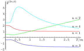
Figure 9: Different two-leg effective couplings at tree-level for $d=3$

FIG. 9 shows the evolution in temperature of the different tree-level effective coupling constants up to $n=4$. We can see that, for temperatures higher than the mass parameter, the effective couplings go smoothly to their known values from the usual dimensional reduction formalism. Nevertheless, for low temperatures, their behavior changes abruptly. The reason for this change is the fact that the functions involved are not analytical in $T$, but we can make expansions in $\mathrm{e}^{-m/T}\ll 1$. If we investigate the high and low $T$ limits for the free propagator, we find that $G_{\phi}(T\rightarrow\infty)^{-1}=\beta\omega^{2}$ and $G_{\phi}(T\rightarrow 0)^{-1}=\omega$. Expanding in soft modes without renormalizing the fields, we obtain that the quadratic part of the effective action will be

$$\Gamma[\Phi]_{\textrm{{\small free}}}\left\{\begin{array}[]{cl}\overrightarrow{\mbox{\scriptsize$T\to\infty$}}&\beta\int_{\bm{x}}\frac{1}{2}\Big{[}(\nabla\Phi)^{2}+m^{2}\Phi^{2}\Big{]}\\ \overrightarrow{\mbox{\scriptsize$T\to 0$}}&\int_{\bm{x}}\Big{[}\frac{1}{2m}(\nabla\Phi)^{2}+m\Phi^{2}\Big{]}+{\cal O}(\nabla^{4}),\end{array}\right.$$

III.3 Soft modes, low temperatures, and small masses

We know that if we start from a massless theory, the thermal bath will provide a temperature dependent mass of the order of the coupling constant, after radiative corrections. Resummation techniques Pisarski (1989); Braaten and Pisarski (1990) include these thermal masses, in order to remove infrared divergences. Other formalisms use small masses in order to regulate the infrared divergences. For example, by starting with a massless theory, then adding a mass term of the order of the perturbation parameter, and subtracting it as part of the interaction Lagrangian Frenkel et al. (1992); Arnold and Zhai (1994).

Consider the scale of the theory $\Lambda$, such that $\underline{m}^{2}\sim\underline{\lambda}<1$, where the underline implies scaling with $\Lambda$: $\underline{m}^{2}=m^{2}/\Lambda^{2}$ and $\underline{\lambda}\equiv\lambda\Lambda^{d-3}$. From dimensional analysis, the different vertex contributions will have the form

$$\gamma^{(2n)}(\bm{p}_{i};T;m;\lambda)=m^{n-d(n-1)}\bar{\lambda}^{n-1}\bar{\gamma}^{(2n)}(\bm{\bar{p}}_{i};\bar{T};\bar{\lambda}),$$ (27)

which can be expanded in the number of loops as

$$\bar{\gamma}^{(2n)}(\bm{\bar{p}}_{i};\bar{T};\bar{\lambda})=\sum_{l=0}\bar{\lambda}^{l}\bar{\gamma}^{(2n,l)}(\bm{\bar{p}}_{i};\bar{T}).$$ (28)

We want to know of which order in $\underline{\lambda}$ are the vertices. As we are interested in soft modes and low temperatures, we must consider them of the order of the mass parameter.

First note that $\bar{\lambda}\sim\underline{\lambda}^{(d-1)/2}$. This implies that for low masses it is not possible to use perturbation theory for $d=1$, as we can see from equation (28). Scaling with $\Lambda$ the external factors in equation (27), we obtain

$$\gamma^{(2n)}(\bm{p}_{i};T;m;\lambda)\sim\underline{\lambda}^{1/2}\bar{\gamma}^{(2n)}(\bm{\bar{p}}_{i};\bar{T};\bar{\lambda})\Lambda^{n-d(n-1)}.$$

The range of convergence of the fields must be $\underline{\Phi}^{2}<1$, from the definition of the cutoff. That is not the case if we renormalize the fields as in equation (26). Expanding in soft modes, considering the external momenta $|\bm{p}|\ll m$ we obtain

$$g^{(2n)}(T,m,\lambda)\sim\underline{\lambda}^{(n+1/2)}\bar{g}^{(2n)}(\bar{T},\bar{\lambda})\Lambda^{2n-d(n-1)},$$

so in this case we need, for convergence, that $\underline{\Phi}_{R}^{2}<\underline{\lambda}^{-1/2}$.

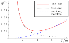
Figure 10: Two-leg effective coupling constant in $d=3$ considering a small mass $m^{2}=\lambda\Lambda^{2}$ at: tree-level (dotted line), one loop (solid line), and one-loop treating the mass as a perturbation (dashed).

As an example, let us compute the one-loop corrected effective coupling $g^{(2)}$ for $d=3$, considering a small mass $m^{2}=\lambda\Lambda^{2}$ calculated in two different ways: one with massive propagators, and the other by considering the mass as a perturbation parameter in the interacting Lagrangian ${\cal L}_{I}=\frac{1}{2}m_{0}^{2}\varphi^{2}+\frac{1}{4!}\lambda_{0}\varphi^{4}$. Following the procedures described for the self-energy, and renormalizing the fields, we derive the result which is shown graphically in FIG. 10. In the case of the one-loop corrected effective coupling (solid line), calculated with the mass included, for lower temperatures it behaves like tree-level (dotted line), as already shown in FIG. 9. As the temperature starts to grow, it behaves like the one-loop corrected effective coupling calculated by considering the mass as a perturbative parameter (dashed line). Therefore, we cannot treat the mass as a perturbation for low temperatures. This is because we have expanded in soft modes for momenta small compared with the mass. When we consider massless propagators, the expansion in momenta must be made by comparing with temperature, so, for lower values of temperature, the expansion does not make sense as can be seen in the propagator, if we consider zero mass and temperature: $G_{\phi}^{-1}\rightarrow p$.

IV Conclusions

We have generalized the rules for the construction of the connected Green functions from the reduced theory, and the construction of the DREA in a simple way. From the two examples of one-loop connected propagators, we show that it is easy to find the temperature independent divergences to be renormalized by the mass and the coupling constant. Also, we identify the Debye mass, which corresponds to the usual thermal mass. The rules can easily be changed to other kinds of field theories.

Maybe the most interesting part of this work is the analysis of the effective action at low temperatures for soft modes. We show graphical examples of different effective coupling constants which for low temperatures change from their extrapolated high temperature behavior due to the non-analytic nature of the functions involved in the temperature. A dimensional analysis of the effective couplings shows us that, for low temperatures, perturbation theory is also valid for $d>1$ if we consider a small mass of the order of the coupling constant. In particular, soft modes, for near-zero temperatures, must be dealt with by including a mass term.

The DREA can, in principle, describe a great variety of low energy theories expanded about the classical limit. The Hamiltonian thus obtained corresponds to a Ginsburg-Landau coarse-grained free energy constructed from a microscopic theory.

In a forthcoming publication, we will use the DREA to analyze a Lagrangian with a small negative mass-squared term, in order to describe a phase transition, and extract critical parameters.

References

- Weinberg (1980) S. Weinberg, Phys. Lett. B91, 51 (1980).
- Ginsparg (1980) P. H. Ginsparg, Nucl. Phys. B170, 388 (1980).
- Appelquist and Pisarski (1981) T. Appelquist and R. D. Pisarski, Phys. Rev. D23, 2305 (1981).
- Nadkarni (1983) S. Nadkarni, Phys. Rev. D27, 917 (1983).
- Zinn-Justin (2000) J. Zinn-Justin (2000), eprint hep-ph/0005272.
- Martin and Schwinger (1959) P. C. Martin and J. S. Schwinger, Phys. Rev. 115, 1342 (1959).
- Kubo (1957) R. Kubo, J. Phys. Soc. Jap. 12, 570 (1957).
- de Carvalho et al. (2001) C. A. A. de Carvalho, J. M. Cornwall, and A. J. da Silva, Phys. Rev. D64, 025021 (2001), eprint hep-th/0101142.
- de Carvalho and Cavalcanti (2002) C. A. A. de Carvalho and R. M. Cavalcanti (2002), eprint hep-th/0210201.
- Amit (1984) D. J. Amit, Field Theory, the Renormalization Group, and Critical Penomena, World Scientific (Singapore, 1984).
- Pisarski (1989) R. D. Pisarski, Phys. Rev. Lett. 63, 1129 (1989).
- Braaten and Pisarski (1990) E. Braaten and R. D. Pisarski, Nucl. Phys. B337, 569 (1990).
- Frenkel et al. (1992) J. Frenkel, A. V. Saa, and J. C. Taylor, Phys. Rev. D46, 3670 (1992).
- Arnold and Zhai (1994) P. Arnold and C.-X. Zhai, Phys. Rev. D50, 7603 (1994), eprint hep-ph/9408276.