Bayesian Statistics at Work: the Troublesome Extraction of the CKM Phase $\alpha$

Abstract

In Bayesian statistics, one’s prior beliefs about underlying model parameters are revised with the information content of observed data from which, using Bayes’ rule, a posterior belief is obtained. A non-trivial example taken from the isospin analysis of $B\rightarrow PP$ ($P=\pi$ or $\rho$) decays in heavy-flavor physics is chosen to illustrate the effect of the naive “objective” choice of flat priors in a multi-dimensional parameter space in presence of mirror solutions. It is demonstrated that the posterior distribution for the parameter of interest, the phase $\alpha$, strongly depends on the choice of the parameterization in which the priors are uniform, and on the validity range in which the (un-normalizable) priors are truncated. We prove that the most probable values found by the Bayesian treatment do not coincide with the explicit analytical solutions, in contrast to the frequentist approach. It is also shown in the appendix that the $\alpha\rightarrow 0$ limit cannot be consistently treated in the Bayesian paradigm, because the latter violates the physical symmetries of the problem.

I Introduction

In Bayesian statistics, probability is a measure of one person’s state of knowledge (also called degree of belief) of the plausibility of a proposition given incomplete knowledge at a given time. Another person may have a different degree of belief in the same proposition, and so have a different probability. The only constraint is that the probabilities chosen by a single person should be consistent (“coherent”): they should obey all the axioms of probability bayesbook . Bayes’ rule is understood as a revision process, by which a prior probability is changed into a new one, the posterior probability, due to input information provided by the data.

The result of any inference problem is the posterior distribution of the quantity of interest. Bayesian models require the specification of prior distributions for all unknown parameters, expressing the actual personal degrees of belief based on all the available information prior to updating one’s degree of belief with the information content of the data. In the case where prior knowledge about model parameters is unavailable, the specification of prior distributions is never unequivocal.

Neither Bayesian statistics nor any other framework provides fundamental rules for obtaining the prior probability about the parameters. The specification of prior distribution may be possible in some simple cases but is impractical in complicated problems if there are many parameters. In practice, especially when nothing or very little is known about the parameters, most Bayesian analyses are performed with so-called “non-informative priors” Kass . An obvious candidate for a non-informative prior is to use a flat prior. The notion of a flat prior is not well-defined because a flat prior of one parameter does not imply a flat prior on a transformed version of that parameter. Prior density distributions are not transformation-invariant, because they depend on the metric. For example, a uniform distribution of $\theta$ does not lead to a uniform distribution of $\mu=\sin(\theta)$. Thus, there is a fair amount of arbitrariness in how ignorance is parameterized, which will affect the posterior probability and hence the result. Moreover, there is a fundamental difference rarely acknowledged between knowing that a uniform prior probability distribution in the range $[\theta_{a},\theta_{b}]$ has been assigned to the value of a parameter $\theta$ as a result of positive knowledge, and not knowing anything about $\theta$ with the exception of its admissible range. These are two fundamentally different states of knowledge. It is often claimed, though without any proof, that the relative prior dependence of the posterior probability distribution is reduced as the statistical information from the measured data is increased.

In the physical sciences, the invariance of conclusions drawn from data under a particular parameter choice is a fundamental concept. Furthermore, it is questionable Mayo “whether scientists have prior degrees of beliefs in the hypotheses they investigate and whether, even if they do, it is desirable to have them figure centrally in learning from data to science. In science, it seems, we want to know what the data are saying, quite apart from the opinions we start out with.”

The mathematical content of this paper being rather simple, its purpose is to illustrate with a concrete use case how strongly prior-dependent the Bayesian treatment can be. The chosen example is taken from the field of particle physics, more specifically from recent results discussed in the domain of $C\!P$ violation. The extraction of the CKM phase $\alpha$ from the isospin analysis of $B\rightarrow PP$ ($P=\pi$ or $\rho$) decays is used as an illustration of a Bayesian analysis at work with flat priors in a multi-dimensional parameter space in presence of mirror solutions. Troublesome results are obtained UTfit1 .

We begin by introducing the analysis formalism and the statistical approaches used to interpret the experimental results. We present the results of the so-called $B\rightarrow\pi\pi$ isospin analysis (see below) in several parameterizations finding that the Bayesian method leads to very different conclusions depending on the choice of the parameterization. We then explicit a simpler two-dimensional example that bears some similarities with the extraction of $\alpha$, namely the existence of mirror solutions, and show why the Bayesian treatment amounts to an unacceptable interpretation of fundamental physics parameters. Finally in appendix we explain in detail the role of the $\alpha\rightarrow 0$ limit, its associated mathematical properties and its relation to $C\!P$ violation and new physics. We show that the Bayesian treatment leads to an unrecoverable divergence when one parameterizes the Standard Model amplitudes by their real and imaginary parts, i.e., when one uses the parameterization that is the most natural from the point of view of the computation of Feynman diagrams. Readers well-aware of the basics of the frequentist and Bayesian statistical treatments may skip Sections III, IV and V.

II Analysis Formalism

The experimental framework consists of the measurement of six observables: three branching fractions and three asymmetries (see, e.g., Ref. babarphysbook ). The three branching fractions are related to the three $B$ meson decays: $B^{0}\rightarrow\pi^{+}\pi^{-}$, $B^{0}\rightarrow\pi^{0}\pi^{0}$, $B^{\pm}\rightarrow\pi^{\pm}\pi^{0}$, where the average is implicitly taken between the two $C\!P$-conjugate decays; $B^{0}$ and $\kern 1.79993pt\overline{\kern-1.79993ptB}{}^{0}$, and $B^{+}$ and $B^{-}$, respectively. The three asymmetries are quantities which would vanish in the absence of $C\!P$ violation (charge conjugation times spatial parity): theses quantities modulate the time dependence of the neutral $B$-meson decays. They are denoted $S^{+-}$, $C^{+-}$ and $C^{00}$.

The use of the isospin analysis to extract fundamental parameters from the $B\rightarrow\pi\pi$ observables is a well known problem that was first solved in 1990 GL . Assuming isospin symmetry (an approximate SU(2) flavor symmetry of the strong interaction, which is known to hold to better than a few percent accuracy), the two pion final state can be represented as a superposition of isospin zero ($I=0$) and isospin two ($I=2$) eigenstates. Within the Standard Model, the $B^{0}$-decay amplitudes can then be written as

$$A^{+-} \equiv A(B^{0}\rightarrow\pi^{+}\pi^{-})=e^{-i\alpha}T^{+-}+P\,,$$

$$\sqrt{2}A^{00} \equiv \sqrt{2}A(B^{0}\rightarrow\pi^{0}\pi^{0})=e^{-i\alpha}T^{00}-P\,,$$ (1)

$$\sqrt{2}A^{+0} \equiv \sqrt{2}A(B^{+}\rightarrow\pi^{+}\pi^{0})=e^{-i\alpha}(T^{00}+T^{+-})\,,$$

where a peculiar phase convention has been taken (in which $q/p$, the $B^{0}\kern 1.79993pt\overline{\kern-1.79993ptB}{}^{0}$ mixing phase shift, is equal to one). The triangular relation $\sqrt{2}A^{+0}=\sqrt{2}A^{00}+A^{+-}$ that follows from the parameterization above is a consequence of the isospin symmetry, and the only information that we have on the amplitudes without any additional hypothesis; the “$P$” (the so-called “penguin”) term in the neutral mode comes from $\Delta I=1/2$ operators that cannot contribute to the $\Delta I=3/2$ charged transition, hence the absence of a “$P$” term in $A^{+0}$. This notation makes explicit the presence of $C\!P$ violation through the $C\!P$-odd weak-interaction phase $\alpha$ (which is the parameter of main interest), while the other (hadronic) parameters are $C\!P$-conserving complex numbers. The $C\!P$-conjugated amplitudes are thus obtained from Eq. (II) by a sign flip $\alpha\rightarrow-\alpha$. In the following, the parameterization from Eq. (II) will be referred to as the “Standard Model” parameterization.

The observables that are currently measured by the $B$-factory experiments BABAR and Belle are the $C\!P$-averaged branching fractions ${\cal B}^{ij}\propto(\tau_{B}/2)(|A^{ij}|^{2}+|\kern 1.79993pt\overline{\kern-1.79993ptA}{}^{ij}|^{2})/2$, where $\tau_{B}$ is the $B^{0}$- or $B^{+}$-meson lifetime depending on the modes, the direct $C\!P$ asymmetries $C^{ij}=(|A^{ij}|^{2}-|\kern 1.79993pt\overline{\kern-1.79993ptA}{}^{ij}|^{2})/(|A^{ij}|^{2}+|\kern 1.79993pt\overline{\kern-1.79993ptA}{}^{ij}|^{2})$ and the $B^{0}\kern 1.79993pt\overline{\kern-1.79993ptB}{}^{0}$-mixing-induced $C\!P$ asymmetry $S^{+-}={\rm Im}(\kern 1.79993pt\overline{\kern-1.79993ptA}{}^{+-}/A^{+-})$. This adds up to six independent constraints on the six independent parameters, namely $\alpha$ and either the modulus and argument, or equivalently the real and imaginary parts, of $T^{+-}$, $T^{00}$ and $P$ (one overall phase being irrelevant, it can be fixed to any value without altering the observables). Thus the system of equations is just constrained. It can be inverted explicitly JC , what will be referred to in the following as the “explicit solution” parameterization. It is assumed throughout this paper that all observables are obtained from Gaussian measurements, and that there is no source of uncertainty other than the unknown tree and penguin amplitudes defined above. The fit of $\alpha$ or of any subset of the unknown parameters is therefore a classical, well-defined, statistical problem.

What makes the isospin analysis an interesting example, besides its non-linearity due to trigonometric functions, is the presence of a high-order exact degeneracy between mirror solutions. Indeed it can be shown explicitly (see, e.g., Ref. JC ) that there are eight parameter sets that give exactly the same value for the observables when one restricts $\alpha$ to the range $[0,\pi]$ (eight other sets are found trivially through the transformation $\alpha\rightarrow\alpha+\pi$, $T^{ij}\rightarrow-T^{ij}$ that leaves the system invariant). Even with infinite statistics, it is not possible from a given set of measurements to determine which of the various mirror solutions is the true one.

The same formalism can be applied (to a good approximation) to the quasi two-body decay $B\rightarrow\rho\rho$. However in this case, only an upper bound on the branching fraction to $\rho^{0}\rho^{0}$ is currently available, which makes the isospin analysis an under-constrained system. It has been shown in the literature GQ ; JC that one obtains bounds on the phase $\alpha$ in such a case.

We consider another useful parameterization of the decay amplitudes, which has been proposed in Ref. LDP . It will be referred to as the “Pivk-LeDiberder” parameterization. One introduces six parameters $\alpha$, $\alpha_{\mathrm{eff}}$, $\mu$, $a$, $\bar{a}$ and $\Delta$ through the definitions

$$A^{+-} = \mu\,a\,,$$

$$A^{00} = \mu\,e^{i(\Delta-\alpha)}\left(1-\frac{a}{\sqrt{2}}\,e^{-i(\Delta-\alpha)}\right)\,,$$

$$A^{+0} = \mu\,e^{i(\Delta-\alpha)},$$ (2)

$$\kern 1.79993pt\overline{\kern-1.79993ptA}{}^{+-} = \mu\,\bar{a}\,e^{2i\alpha_{\mathrm{eff}}}\,,$$

$$\kern 1.79993pt\overline{\kern-1.79993ptA}{}^{00} = \mu\,e^{i(\Delta+\alpha)}\left(1-\frac{\bar{a}}{\sqrt{2}}\,e^{-i(\Delta+\alpha-2\alpha_{\mathrm{eff}})}\right)\,,$$

$$\kern 1.79993pt\overline{\kern-1.79993ptA}{}^{+0} = \mu\,e^{i(\Delta+\alpha)}\,.$$

The above description is the simplest one that makes explicit the two crucial ingredients of the isospin analysis, namely the triangular relation between the amplitudes and the fact that $2\alpha$ is the phase difference between $\kern 1.79993pt\overline{\kern-1.79993ptA}{}^{+0}$ and $A^{+0}$.

III Frequentist Analysis

“Frequentist statistics provides the usual tools for reporting objectively the outcome of an experiment without needing to incorporate prior beliefs concerning the parameter being measured or the theory being tested. As such they are used for reporting essentially all measurements and their statistical uncertainties in High Energy Physics” pdg2005 . The Frequentist sees probability as the long-run relative frequency of occurrence. Hence, the frequentist analysis assumes that a population mean is real, but unknown, and unknowable, and can only be estimated from the available data.

We neglect in the following the occurrence of physical boundaries for the true values which greatly simplifies the computation of frequentist confidence levels. We adopt a $\chi^{2}$-like notation and define

$$\chi^{2}(\theta)\equiv-2\ln({\cal L}_{\{\mathbf{x}\}}(\theta))\,,$$ (3)

where the likelihood function, ${\cal L}$, quantifies the agreement between the measured observables, $\{\mathbf{x}\}$, and their theoretical counterparts, $\{\mathbf{f}(\theta)\}$. The $\theta$ parameters are the unknowns of the theory, e.g., for the Pivk-LeDiberder parameterization one has $\theta=\{\alpha,\alpha_{\rm eff},\mu,a,\bar{a},\Delta\}$.

Under these assumptions, and neglecting experimental correlations, the likelihood components of ${\cal L}$ are independent Gaussian distribution functions

$${\cal L}_{\{x_{i}\}}(\theta)\propto{1\over\sigma_{i}}\,{\rm exp}\left[-{1\over 2}\left({x_{i}-f_{i}(\theta)\over\sigma_{i}}\right)^{\!\!2\,}\right]\,,$$ (4)

each with a standard deviation given by the statistical uncertainty $\sigma_{i}$ on the measurement $i$. In this case, using incomplete $\Gamma$ functions (as computed, e.g., with ”${\rm Prob}$” the well known routine from the CERN library), one can infer a confidence level (CL) from the above $\chi^{2}$ value as follows

$${\rm CL} = {\rm Prob}(\chi^{2}(\theta),N_{\rm dof})~{},$$ (5)

$$= \frac{1}{\sqrt{2^{N_{\rm dof}}}\Gamma({N_{\rm dof}}/2)}\int\limits_{\chi^{2}(\theta)}^{\infty}e^{-t/2}t^{N_{\rm dof}/2-1}\,dt\,.$$

IV Bayesian Analysis

Bayesian probability, also named personal probability or (more often but less appropriately) subjective probability, represents one’s degree of belief. It is thus a summary of one’s own opinions about an uncertain proposition, not something inherent to the system being studied. Thus, in the personalistic Bayesian approach, hypotheses or unknowns can never be directly measured or statistically evaluated. A personal probability statement cannot be proved or disproved, verified or falsified.

A posterior probability density function (PDF), $P(\mathbf{\theta}|\{\mathbf{x}\})$, for a model parameter $\theta$ having observed the data $\{\mathbf{x}\}$ is, using the Bayes’ rule:

$$P(\theta|\{\mathbf{x}\})=\frac{P(\{\mathbf{x}\}|\theta)\pi(\theta)}{\int P(\{\mathbf{x}\}|\theta)\pi(\theta)d\theta}\,,$$ (6)

where $P(\{\mathbf{x}\}|\theta)$ is nothing more than the likelihood function (${\cal L}_{\{\mathbf{x}\}}(\theta)$) of the true parameter value $\theta$ taken at the observed data $\{\mathbf{x}\}$. The posterior PDF in $\theta$ is obtained by multiplying ${\cal L}$ by the prior PDF $\pi(\theta)$, the probability density function for the model parameter $\theta$. In essence, the prior is reweighed according to the likelihood of the data.

It should be emphasized here that the probability associated with the value of a model parameter cannot be interpreted meaningfully as a frequency of an outcome of a repeatable experiment. Instead, it is understood to reflect the degree of belief that the parameters have particular values. Stated otherwise, since the parameter $\theta$ is not a random variable, the probability distribution for $\theta$ is not a probability distribution in the usual frequency sense, i.e., one cannot sample from this distribution and obtain various values for $\theta$ Porter . However, the prior PDF $\pi(\theta)$ can be defined with the formal rules of probabilities and quantifies one’s degree of belief about the parameter before carrying out the experiment, i.e., no matter what the data are. There is no fundamental recipe for assigning a priori probabilities to parameters. Bayes’ rule, after choosing a certain prior $\pi(\theta)$, only states how the a posteriori probability changes in the light of the existing experimental data. In other words, Bayesian posterior PDF depends not only on the observation itself, but also on the state of knowledge and beliefs of the observer. As a consequence, the posterior PDF by itself does not in general provide a useful summary of the result of the experiment, as it convolves the data with the personal beliefs needed to construct the prior PDF.

In the case of more than one parameter, $\theta_{1},\ldots,\theta_{m}$, the a posteriori PDF of, say the parameter $\theta_{1}$, is obtained by integrating out the parameters $\theta_{2},...,\theta_{m}$ to get the marginal PDF

$$P(\theta_{1}|\{\mathbf{x}\})=\int\!P(\theta_{1},\theta_{2},\ldots,\theta_{m}|\{\mathbf{x}\})d\theta_{2}\ldots d\theta_{m}\,.$$ (7)

By doing so, one has chosen a certain parameterization ($\theta_{1},\ldots,\theta_{m}$) and a corresponding metric ($d\theta_{1}\ldots d\theta_{m}$).

V Priors

Non-informative prior distributions are generally improper (they do not normalize) when the parameter space is not compact which may lead to an improper posterior. However, a posterior must always be proper, in other words, it must be a probability (discrete parameter) or a PDF (continuous parameter). To remedy this problem what is done in practice is to truncate the range of the prior. However, the ranges for the prior PDF with $\pi(\theta)\neq 0$ restrict the allowed range for the posterior PDFs in $P(\theta|\{\mathbf{x}\})$. Hence, it has to be verified that the a priori ranges do not introduce a cut in the posterior PDF. If this, however, is the case one needs to either enlarge the ranges of the prior PDF where $\pi(\theta)\neq 0$, or to justify the ranges used.

In an ideal case, the posterior PDF should not depend on the prior PDF but only on the experimental likelihood. However, in reality, the choice of prior always matters. Belief is not easily measured with high accuracy. The extent of approximation hidden in the prior densities is seldom considered in Bayesian analyses. What is sometimes suggested is to perform a robustness analysis bayesbook (sensitivity analysis of the posterior by considering, individually, the effects of a small number of potential alternative choices of a model component, such as parameterization or prior distribution). However, this concept is not well-defined. It lacks a criterion of what is an acceptable change of the posterior and also which class of priors should be used.

It is often stated that the data swamp the prior: the prior is washed out as the number of observation increases. The statement of the “washing out” of the prior lacks a qualitative and also quantitative proof and would need to be verified case-by-case. Furthermore, the possibility of eventual convergence of belief is irrelevant to the day-to-day problem of learning from data in science. Moreover, it provides only an illusion of the existence of an objective probability probaphilo1 (the eventual convergence of opinions by remaining coherent (internal consistency with the probability axioms) is not enough to guarantee that the Bayesian answer is a good answer to a real-world question).

We cannot verify if the Bayesian probability $P(\theta|\{\mathbf{x}\})$ is “correct” by observing the frequency with which $\theta$ occurs, since this is not the way Bayesian probability is defined. Hence, it would be odd trying to justify post hoc the priors on frequentist grounds Cousins00 .

Let us illustrate with a very simple educated scenario how (precise) posterior results can be solely “determined” by the multidimensional convolution of prior probability densities. For instance, we may consider a $N$-dimensional parameter space $x_{i}$, with $i=1,2,...N$, with $0<x_{i}<1$, in which no experimental input is known for the values of the $x_{i}$: one knows nothing at all. Still, even in such a total absence of knowledge, a Bayesian treatment can pretend powerful constraints. If one is interested in the radius $R=\sqrt{\sum_{i=1}^{N}x_{i}^{2}}$ where lies the true set of model parameters, the Bayesian answer is clear. It is shown in Fig. 1, for $N=6$, and for the “reasonable” choice of flat priors. One finds $R=1.39\pm 0.27$, where the central value corresponds to the mean radius and the errors give the symmetric 68% posterior probability interval around the mean value. One has achieved the remarkable feat of learning something about the radius of the hypersphere, whereas one knew nothing about the Cartesian coordinates and without making any experiment.

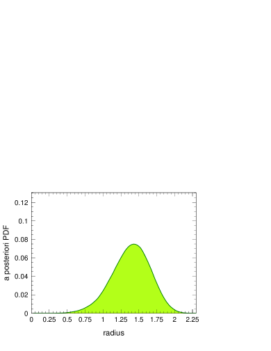
Figure 1: Bayesian posterior PDF of the radius $R=\sqrt{\sum_{i=1}^{6}x_{i}^{2}}$ in a six-dimensional parameter space where no experimental input is known for the values of the $x_{i}$, and where the “reasonable” choice of flat priors for the $x_{i}$, with $0<x_{i}<1$, has been used. The Bayesian treatment succeeds to constrain the radius.

VI Parameterizations

Table 1: Ranges taken for the parameters of the various parameterizations used in this paper to fit the $B\rightarrow\pi\pi$ observables. The ranges for the MA, PLD and ES parameterizations are chosen such that they fully contain the posteriors for all parameters (see Fig. 3). The ranges for the RI parameterization are chosen similar to the ones in the MA parameterization. The choice of the ranges in the RI parameterization will be further discussed in Appendix B.3. The phases are given in radians.

MA param.			RI param.			PLD param.			ES param.
	min.	max.		min.	max.		min.	max.		min.	max.
	value	value		value	value		value	value		value	value
$|T^{+-}|$	0	10	$|T^{+-}|$	0	15	$a$	0.4	1.2	${\cal B}^{+-}(10^{-6})$	3	7
$|P|$	0	10	$\mathrm{Re}(P)$	$-10$	10	$\bar{a}$	0.8	1.6	${\cal B}^{+0}(10^{-6})$	3	8
$|T^{00}|$	0	10	$\mathrm{Im}(P)$	$-2.5$	0	$\mu$	1.6	2.6	${\cal B}^{00}(10^{-6})$	0	3
$\delta_{P}$	0	$2\pi$	$\mathrm{Re}(T^{00})$	$-10$	5	$\delta$	0	$2\pi$	$C^{+-}$	$-0.8$	0.2
$\delta_{00}$	0	$2\pi$	$\mathrm{Im}(T^{00})$	$-4$	4	$\alpha_{\rm eff}$	0	$2\pi$	$S^{+-}$	$-1$	0
$\alpha$	0	$\pi$	$\alpha$	0	$\pi$	$\alpha$	0	$\pi$	$C^{00}$	$-1$	1

In this section we consider the Bayesian treatment applied to $B\rightarrow\pi\pi$ decays (the Bayesian treatment of $B\rightarrow\rho\rho$ decays is discussed in Appendix A). The current world average values for the observables are ${\cal B}^{+-}=(5.1\pm 0.4)\times 10^{-6}$, ${\cal B}^{+0}=(5.5\pm 0.6)\times 10^{-6}$, ${\cal B}^{00}=(1.45\pm 0.29)\times 10^{-6}$, $C^{+-}=-0.37\pm 0.10$, $S^{+-}=-0.50\pm 0.12$, $C^{00}=-0.28\pm 0.40$  pipi . These observables are reproduced by the model with the following eight values for the phase $\alpha$ (in degrees), as computed from the analytical solutions in Footnote 2:

$$\{6.3,83.7,91.8,120.7,128.8,141.2,149.3,178.2\}\,.$$ (8)

We apply the Bayesian treatment using the four parameterizations in Section II:

• the Standard Model modulus and argument parameterization (MA);

• the Standard Model real and imaginary parameterization (RI);

• the Pivk-LeDiberder parameterization (PLD);

• the explicit solution parameterization (ES).

Obviously, one may consider a much larger variety of parameterizations, but the ones considered here are sufficient to make our point clear. They are all natural in the sense that they were defined beforehand without having in mind the present discussion. For all four parameterizations we use uniform priors for all the six model parameters. In particular, the prior PDF used for $\alpha$ is uniform in the range [$0,\pi$] for the MA, RI and PLD parameterizations (for the ES parameterization, $\alpha$ is not an input model parameter). The choice of uniformity is not the result of a strong argument, nor is it particularly natural; rather it is taken for the sake of simplicity, and to be conform to the choice made by Bayesian analyses already published on the subject UTfit1 . The ranges used for the parameters are given in Table 1. The resulting posterior PDFs for $\alpha$ are shown in Fig. 2 (the posterior PDFs for the other model parameters are shown in Fig. 3). The top plot gives the $1-{\rm CL}$ result for the frequentist treatment. It is independent of the parameterization used. The eight solutions in Eq. (8) for the phase $\alpha$ are clearly visible, and correspond exactly to the analytical solutions in Footnote 2.

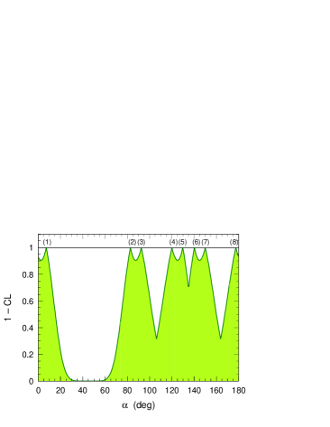
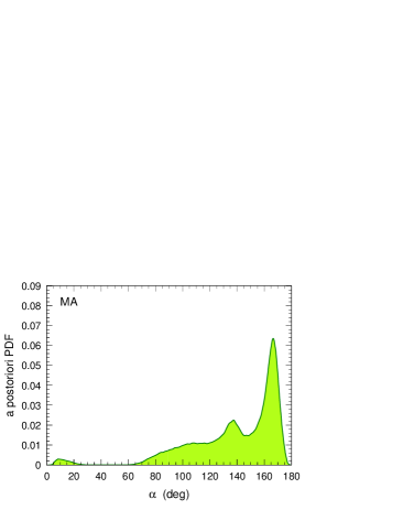
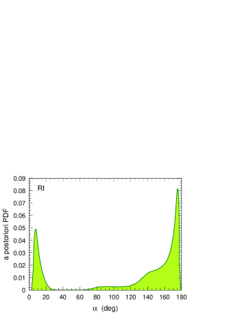
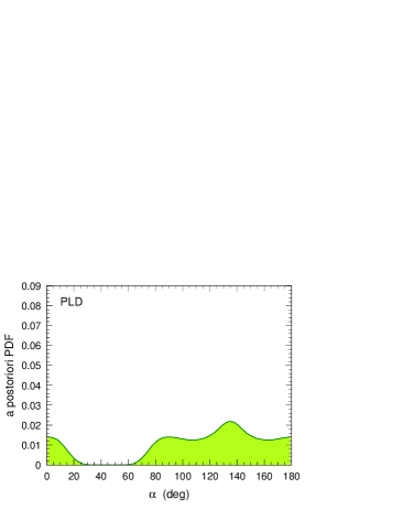
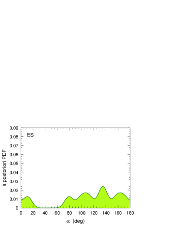
Figure 2: Results for the CKM phase $\alpha$ obtained with the different parameterizations from the $B\rightarrow\pi\pi$ isospin analysis. The upper plot shows the frequentist confidence level, which is independent of the parameterization used. The solutions (1) through (8) coincide with the analytical solutions computed from the expressions given in Footnote 2. The remaining plots show the Bayesian a posteriori PDFs for the parameterizations indicated by the labels. The posterior PDF in the RI parameterization depends strongly on the ranges chosen for the priors of $|T^{+-}|$, ${\rm Re}(P)$ and ${\rm Re}(T^{00})$ parameters (see Appendix B.3).

VI.1 Modulus and Argument Parameterization

The Bayesian treatment indicates the presence of basically two mirror solutions; the previous mirror solution at $\alpha\simeq 135^{\circ}$ and a new solution, which is strongly favored, at $\alpha\simeq 165^{\circ}$. One also observes that values nearby $0^{\circ}$ and $180^{\circ}$ are excluded in this parameterization, in contrast with the following parameterizations. In the Bayesian approach, all the information resides in an individual’s posterior probability, the posterior PDF for $\alpha$ must be read as the individual’s updated belief in the plausible values of the parameter $\alpha$. The individual’s degree of belief is thus higher for a value of $\alpha\simeq 165^{\circ}$ than for $\alpha\simeq 135^{\circ}$.

VI.2 Real and Imaginary Parameterization

The Bayesian treatment seems to detect the presence of two mirror solutions, a mirror solution at $\alpha\simeq 10^{\circ}$ and another solution, which is favored, at $\alpha\simeq 175^{\circ}$. The posterior PDF appears to vanish at the origin (and at $180^{\circ}$). However, this is only an artifact resulting from the truncation of the prior ranges used for $|T^{+-}|$, ${\rm Re}(P)$ and ${\rm Re}(T^{00})$ (see Footnote 10). As demonstrated in Appendix B.3 the posterior diverges for $\alpha=0^{\circ}\,(180^{\circ}$) and is not normalizable. Expanding the ranges leads to an improper posterior for $\alpha$.

VI.3 Pivk-LeDiberder Parameterization

The Bayesian treatment only vaguely detects the presence of mirror solutions. The posterior PDF tends to favor a value for $\alpha$ ($135^{\circ}$) which corresponds to a dip in the frequentist $1-{\rm CL}$. This is a hint that the Bayesian treatment introduces a piece of information which is “missed” by the frequentist analysis. Since the latter uses all the available experimental data, this additional piece of information must be embedded in the priors. One also observes that values nearby $0^{\circ}$ and $180^{\circ}$ are not disfavored.

MA parameterization — a posteriori PDFs                         RI parameterization — a posteriori PDFs
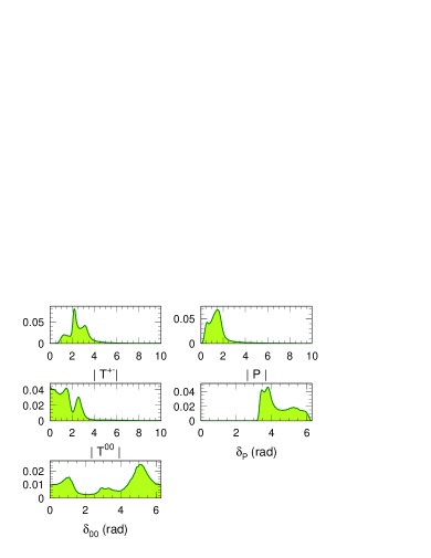
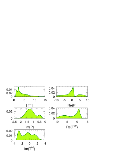
PLD parameterization — a posteriori PDFs                        ES parameterization — a posteriori PDFs

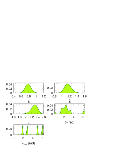
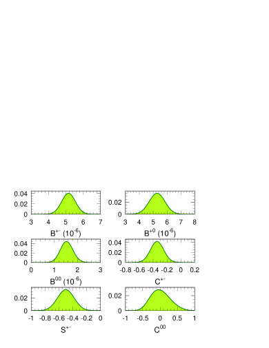
Figure 3: Posterior PDFs for the various model parameters used in this paper except for $\alpha$ which are shown in Fig. 2. One observes that for the RI parameterization the posterior PDFs for ${\rm Re}(P)$ and ${\rm Re}(T^{00})$ do not vanish at the lower edge of their ranges so the ranges should be expanded further. Although the $|T^{+-}|$ posterior appears to be contained in its prior range, it turns out that it must also be expanded further. More generally, as illustrated by the RI parameterization, for the sake of consistency, a Bayesian treatment must provide the proof that the range chosen for the priors are not introducing hidden piece of information. It is shown in Appendix B.3 that for the RI parameterization the choice of the ranges actually determines the posterior PDF for $\alpha$.

VI.4 Explicit Solution Parameterization

The Bayesian treatment detects the presence of mirror solutions, but like in the PLD parameterization, one solution is favored for $\alpha$ ($135^{\circ}$). The fact that one solution is favored over the others is because two nearby mirror solutions are superimposed in the Bayesian treatment (see Section VIII). This feature is present in all parameterizations. In the RI parametrization, it is reflected only as a shoulder in the posterior PDF. One also observes that values nearby $0^{\circ}$ and $180^{\circ}$ are not disfavored. The posterior PDF for $\alpha$ is akin to the one obtained with the PLD parameterization. This is because the latter parameterization is chosen close to the measured quantities.

VI.5 Conclusion

The Bayesian PDFs result from a prior- and parameterization-dependent weighted average of data with mirror solutions. The fact that the posterior PDFs in the MA and RI parameterizations are so different compared to the PLD and ES parameterizations is due to a strong prior dependence. The behavior of the posterior PDF at the origin (and at $180^{\circ}$) also strongly depends on the parameterization (see Appendix B).

From all these results, what is a scientist supposed to communicate as a value for the parameter $\alpha$, without forgetting that they are all based on the same data? Bayesianism is simply a system for keeping one’s internal beliefs self-consistent. It is not concerned with whether or not these beliefs represent the information content of the data.

VII Removing Essential Information

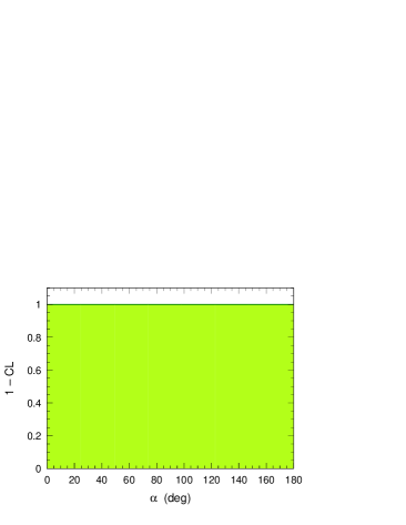
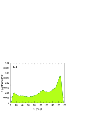
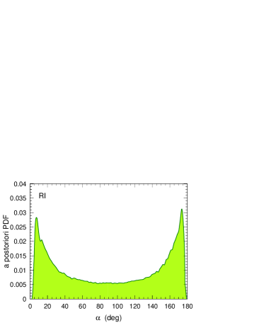
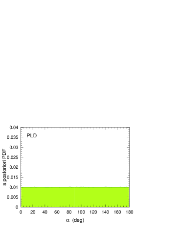
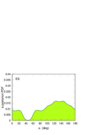
Figure 4: Results for the CKM phase $\alpha$ obtained with the different parameterizations from the $B\rightarrow\pi\pi$ isospin analysis, without using the input from the $B^{0}\rightarrow\pi^{0}\pi^{0}$ branching fraction and direct $C\!P$-asymmetry measurements. No model-independent constraint on $\alpha$ can be inferred in this case (with the exception of the exclusion of the singular points $\alpha=0,\pi$). The upper plot shows the frequentist confidence level, which is independent of the parameterization used. The remaining plots show the Bayesian a posteriori PDFs for the parameterizations indicated by the labels (the unsmooth aspect of some PDFs is due to the fact that we used “only” $10^{10}$ (sic!) Monte Carlo events to carry out the numerical integration).

It is instructive to study the behavior of the Bayesian posteriors in a situation where one deliberately removes crucial data from the analysis, e.g., when performing the fit without using the $B^{0}\rightarrow\pi^{0}\pi^{0}$ branching fraction and direct $C\!P$-asymmetry measurements. In this case it is well known babarphysbook that no information on $\alpha$ can be derived from the data (with the exception of the exclusion of $\alpha=0$ in case of non-zero $C\!P$ violation, see Appendix B.1). In effect, having carried out the fit for a given $\alpha$ value, the values of the model parameters that correspond to this fit can be used to compute explicitly the values of the model parameters corresponding to any other value of $\alpha$, if non-zero (see Appendix B.1): this second set of values yields a fit of exactly the same quality ($\chi^{2}$). Stated differently, the posterior for $\alpha$ provided by the Bayesian treatment, if unbiased, must be uniform since data do not favor any value of $\alpha$. The posterior PDF obtained for the four parameterizations are shown in Fig. 4. While the PLD parameterization yields the expected uniform PDF, the three others do not: they are able to extract information on $\alpha$, which is introduced by the priors.

VIII Mirror solutions in a simple 2D problem

In this section we present a simple and solvable two-dimensional example to illustrate how mirror solutions make the Bayesian approach fail. We work within a theory that predicts the expressions of two observables $X$ and $Y$ as a function of the two parameters $\alpha$ and $\mu$

$$X = (\alpha+\mu)^{2}\,,$$

$$Y = \mu^{2}\,.$$ (9)

Assuming $(X_{m},Y_{m})$ are measured values for the observables, the central values for the parameters can be found by inverting the above system

$$\alpha_{0} = \epsilon_{X}\,\sqrt{X_{m}}-\epsilon_{Y}\,\sqrt{Y_{m}}\,,$$ (10)

$$\mu_{0} = \epsilon_{Y}\,\sqrt{Y_{m}}\,,$$

where $\epsilon_{X},\,\epsilon_{Y}=\pm 1$. Hence there are in general four solutions for $(\alpha_{0},\mu_{0})$ for a given set of measurements. Note that this example is far from being academic, since the theoretical expressions above are very similar to the usual amplitudes $\leftrightarrow$ branching fraction relations in particle physics. The pattern of discrete ambiguities is also very similar to the one encountered in the isospin analysis for the CKM phase $\alpha$.

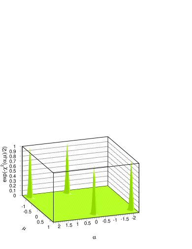
Figure 5: 2D example (Eqs. (9) and (11)): the values of $\exp(-\chi^{2}/2)$ as a function of the parameters $(\alpha,\mu)$.

If $\alpha$ and $\mu$ are fundamental physics parameters, Nature can only accommodate a single pair of values. This means that the representation of the four-valued discrete ambiguity $(\epsilon_{X},\,\epsilon_{Y})=(+1,+1)\,,(+1,-1)\,,(-1,+1)\,,(-1,-1)$ must be interpreted as a logical exclusive OR operator.

We assume that an experiment has measured the observables from a Gaussian sample of events, with the results

$$X = 1.00\pm 0.07\,,$$

$$Y = 1.10\pm 0.07\,.$$ (11)

While the measurement is reasonably precise (below the 10% level), and the mirror solutions are well separated in the $(\alpha,\mu)$ space (see Fig. 5), the central values correspond to a somewhat “unlucky” situation since, as shown in Fig. 6,

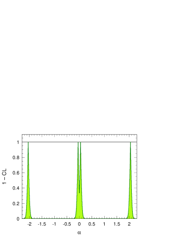
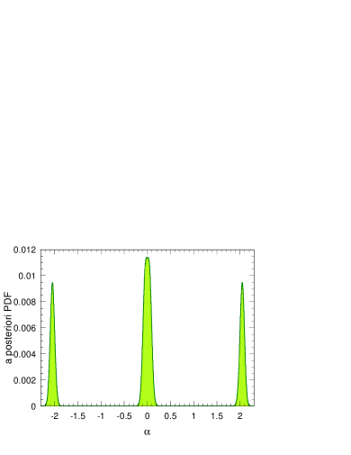
Figure 6: Top: result of the frequentist fit to the data. The peaks are exactly located at the analytical solutions $\alpha=-2.05$, $-0.05$, $0.05$, $2.05$ computed from Eq. (10). Bottom: a posteriori PDF according to the Bayesian treatment. The most probable value is biased.

.

the two solutions for small $\alpha$ overlap somewhat. This kind of overlapping precisely corresponds to what may occur in the isospin analysis of the $B\rightarrow\pi\pi$ data.

The result of the Bayesian procedure applied to this 2D example is shown in Fig. 6. One immediately sees the striking difference with respect to the frequentist fit: after the marginalization with respect to the nuisance parameter $\mu$, only one peak instead of two is left close to the origin in the $\alpha$ constraint, and its best value is biased with respect to the minimum $\chi^{2}$ ones (which coincide with the explicit solution of Eq. (10)).

This unexpected behavior is best understood by looking at Fig. 5. In this space the likelihood is Gaussian and the four solutions do not overlap; while the minimum-$\chi^{2}$ fit selects, for each value of $\alpha$, the best value of $\mu$ with respect to the data, the Bayesian procedure integrates BonaFLHC all events in the $\mu$ direction that correspond to the same value of $\alpha$. In other words, the frequentist approach naturally implements the logical exclusive OR operating on the solutions, in contrast to the Bayesian approach that effectively replaces OR by AND. The latter is clearly unacceptable if one is used to the common wisdom that fundamental parameters have a definite single value realized in Nature. In the present case, the counter-intuitive result of the Bayesian procedure is that the most probable value of $\alpha$ is $\alpha=0$, which in turn implies $X=Y$ that is not the situation preferred by the data (see Eq. (11)).

IX Origin of the problem

The origin of the problem lies in the very first Bayesian assumption, namely that unknown model parameters are to be understood as mathematical objects distributed according to PDFs, which are assumed to be known: the priors. Obviously, the choice of the priors cannot be irrelevant; hence, the Bayesian treatment is doomed to lead to results which depend on the decisions made, necessarily on unscientific basis, by the authors of a given analysis, for the choice of these extraordinary PDFs. This is not a new situation. This limitation — deliberately mixing information coming from scientific data together with human inputs — is frequently perceived as mild, because “reasonable variations” of the human inputs lead to “reasonable variations” of the output of the Bayesian treatment. Moreover, a particular shape of PDF is declared to be “reasonable”: the uniform PDF. This is because, implicitly, one feels that using a flat distribution for priors is akin to using no information at all, hence injecting only a weak a priori assumption through the priors.

What “reasonable variations” means is no more no less clear as what “systematics uncertainties” systematics mean in general: the dependence on the priors can be viewed as a systematic uncertainty of human origin. What is particular in the Bayesian treatment discussed in this article is that “reasonable variations” of the human inputs lead to clearly “unreasonable variations” of the output of the Bayesian treatments. For example, the posterior PDF for $\alpha$ (see Fig. 2) using the RI parameterization (with the ranges of Table 1) leads one to conclude that the Standard Model is close to being defeated; knowing that the bulk of data (from other $B$ decays) indicates a value of the phase $\alpha=(100^{+15}_{-9})^{\circ}$ jerome:fpcp06 . Worse, if one widens to infinity the ranges used for the RI parameterization, the Bayesian treatment fails to provide a proper PDF for $\alpha$ (see appendix B.3). The key here is that the statistical analysis dealt with is performed in a multivariate parameter space. It is well known that the naive use of “uninformative” priors, especially in multivariate spaces, suffer from various paradoxes and is thus widely criticized in the literature Kass ; Seidenfeld . Our examples are even more striking because of strong non-linearities and exact degeneracy among several mirror solutions, and show that the analysis presented in Ref. UTfit1 bears no physical meaning.

X Conclusion

We have demonstrated in this paper that in the isospin analysis of $B\rightarrow\pi\pi$ decays used to constrain the CKM phase $\alpha$, despite the rather precise experimental inputs, the posterior PDF for $\alpha$ shows a striking dependence on shape and ranges used for the prior PDFs, and on the choice of the amplitude parameterization. The very frequent naive use of flat priors as presumed “non-informative” priors hides important unwarranted assumptions, which may easily invalidate the analysis. As stressed by David R. Cox at the Phystat05 conference cox : “It seems to be agreed from all theoretical standpoints that flat or ignorance priors are dangerous, although they are widely used [in Bayesian statistics]. Flat priors in several dimensions may produce clearly unacceptable answers.” Flat priors are informative. There is a big difference between no knowledge, and a distribution that is uniform in some (arbitrary) parameterization. Contrary to what is often stated, Bayesian and frequentist statistics can lead to very different conclusions about the same data, even in the limit of a large data sample. The choice of priors always matters in the Bayesian treatment.

The proponents for the use of Bayesian statistics in High Energy Physics often argue that ”everybody is Bayesian in everyday life”. It is certain that Bayesian reasoning dominates the decision making mechanism of our everyday life. Scientific results however differ in many aspects from everyday-life reasoning. In particular, the translation of prior beliefs into a robust posterior number, representing universal knowledge is impossible. Only the exact knowledge of all prior assumptions (including the parameterization, PDF shapes and parameter ranges) used in a certain Bayesian analysis allows another one to reproduce its posterior result. Bayesian statistics has been shown to be useful for decision making, such as buying and selling stock options, or filtering out unwanted electronic mails. The decision-making problem is not scientific in nature.

Table 2: Ranges taken for the parameters of the various parameterizations used to fit the $B\rightarrow\rho\rho$ observables. The phases are given in radians.

MA param.			RI param.			PLD param.			ES param.
	min.	max.		min.	max.		min.	max.		min.	max.
	value	value		value	value		value	value		value	value
$|T^{+-}|$	0	10	$|T^{+-}|$	0	40	$a$	0.8	2.4	${\cal B}^{+-}(10^{-6})$	10	45
$|P|$	0	10	$\mathrm{Re}(P)$	$-35$	35	$\bar{a}$	0.8	2.4	${\cal B}^{+0}(10^{-6})$	0	30
$|T^{00}|$	0	10	$\mathrm{Im}(P)$	$-8$	8	$\mu$	2.2	4.5	${\cal B}^{00}(10^{-6})$	0	2.5
$\delta_{P}$	0	$2\pi$	$\mathrm{Re}(T^{00})$	$-40$	10	$\delta$	0	$2\pi$	$C^{+-}$	$-0.6$	0.6
$\delta_{00}$	0	$2\pi$	$\mathrm{Im}(T^{00})$	$-8$	8	$\alpha_{\rm eff}$	0	$2\pi$	$S^{+-}$	$-1$	1
$\alpha$	0	$\pi$	$\alpha$	0	$\pi$	$\alpha$	0	$\pi$	$C^{00}$	$-1$	1

Leonard J. Savage, a founder of modern subjective Bayesianism makes very clear throughout his work that the theory of personal probability “is a code of consistency for the person applying it, not a system of predictions about the world around him”. “But is a personal code of consistency, requiring the quantification of personal opinions, however vague or ill formed, an appropriate basis for scientific inference?” Mayo . Isn’t a hypothesis in physical science either true or false? What is hence the meaning of the prior in this case? The Bayesian personal probability theory misses the main point: “it confuses feeling with fact” probaphilo2 . In physical sciences, the theory is intended to describe the external physical universe, rather than one’s internal psychological state.

Science has to summarize the available information the best it can. The Bayesian tools do not tell us what we want to know in science. What we seek are methods for generating and analyzing data and for using data to learn about experimental processes in a reliable manner. The kinds of tools needed to do this are crucially different from those the Bayesian statistics supplies Mayo . These difficulties with the personalistic Bayesian approach indicate that there is a need for objective probabilities and a methodology for statistics based on testing. However the test statistics is chosen allows for an objective interpretation of the scientific results CoxMayo .

Appendix A Bayesian treatment applied to $B\rightarrow\rho\rho$ decays

The (longitudinally polarized) $B\rightarrow\rho\rho$ system is similar to $B\rightarrow\pi\pi$ except that only an upper bound on the branching fraction to $\rho^{0}\rho^{0}$ is currently available. The current world average values for the observables are ${\cal B}^{+-}=(25.1\pm 3.7)\times 10^{-6}$, ${\cal B}^{+0}=(19.1\pm 3.5)\times 10^{-6}$, ${\cal B}^{00}=(0.54\pm 0.41)\times 10^{-6}$, $C^{+-}=-0.02\pm 0.17$, $S^{+-}=-0.22\pm 0.22$ rhorho (the longitudinal polarizations are $f^{+-}=0.966\pm 0.025$ and $f^{+0}=0.96\pm 0.06$). The ranges for the flat prior PDFs in the various parameterizations are summarized in Table 2. The resulting posterior PDFs for $\alpha$ are shown in Fig. 7. Again the frequentist treatment (see top plot in Fig. 7) is independent of the parameterization used. The constraints on $\alpha$ are lumped together under the two plateaus in the 1-CL curve.

In the PLD and ES parameterizations, the range of plausible values for the parameter $\alpha$ respect the symmetry of the problem. As explained in Appendix B.1, the experimental data are still consistent with no $C\!P$ violation, so the posterior PDF for $\alpha=0[\pi]$ does not vanish. However, in the Standard Model parameterization, the prior breaks the symmetry of the problem and leads to a disaster in the RI parameterization (see discussion in Appendix B.3). In both cases, information contained in the data are convolved with additional information provided by the priors: the posterior is dominated by the priors and not by the data.

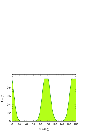
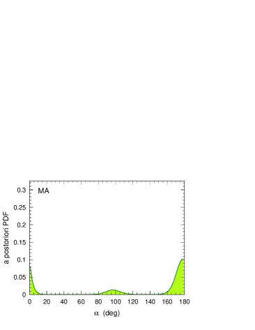
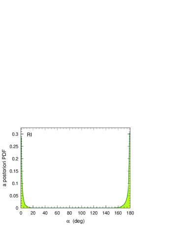
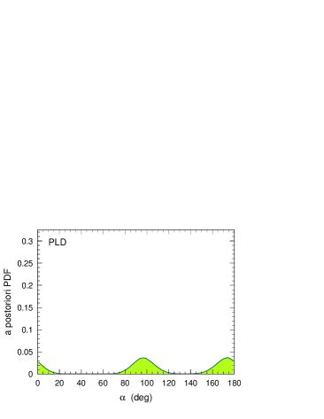
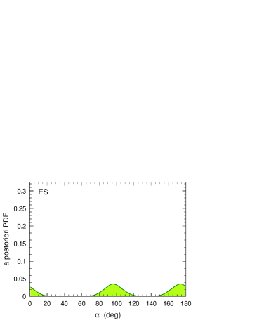
Figure 7: Results for the CKM phase $\alpha$ obtained with the different parameterizations from the $B\rightarrow\rho\rho$ isospin analysis. The upper plot shows the frequentist confidence level, which is independent of the parameterization used. The remaining plots show the Bayesian a posteriori PDFs for the parameterizations indicated by the labels.

Appendix B The $\alpha\rightarrow 0$ limit

In the next two sections, we present two additional parametrizations that describe finite $C\!P$ violation with $\alpha=0$ and finite values for the remaining parameters, and that are mathematically equivalent to the Standard Model parametrization except at $\alpha=0$.

B.1 Mathematics

The point $\alpha=0\ [\pi]$ is a particular point of the theory for physical reasons. In the Standard Model it corresponds to vanishing $C\!P$ violation. The compatibility of the current $B\rightarrow\pi\pi$ data with this point is only marginal, because the $C\!P$ asymmetries are found to be different from zero pipi ; hfag .

As described in Sections III and IV, the behavior of the two statistical approaches around $\alpha=0\ [\pi]$ shows striking differences. In the $B\rightarrow\pi\pi$ case, the frequentist method provides no significant exclusion confidence level for values of $\alpha$ close to zero (the fact that Fig. 2 (upper plot) depicts a continuous $1-{\rm CL}$ line through the point $\alpha=0$ is an artifact of the chosen binning of the $\alpha$ scan that does not hit this singular point). Setting $\alpha$ to zero in the Standard Model parameterization leads to a confidence level of the order of $10^{-8}$, which reflects the presence of $C\!P$ violation in the data. The frequentist confidence level as a function of $\alpha$ is thus discontinuous, as explained below and in Appendix B.2.

On the other hand, whatever the values of the observables, the PDF as a function of $\alpha$ is continuous at the origin in the Bayesian approach, and exhibits a clear drop in the MA parameterization. In the $\rho\rho$ case, where the experimental data are still compatible with the absence of $C\!P$ violation, the $\alpha=0\ [\pi]$ value has a fairly good PDF/CL in both Bayesian and frequentist methods (with however the usual strong prior dependence for the Bayesian result).

The fact that vanishingly small, but non zero, values of the $C\!P$ phase $\alpha$ can generate finite $C\!P$ violation is easily seen as follows. Let us take the branching fraction $\cal{B}^{+-}$ and $C\!P$ asymmetry $C^{+-}$ as an example: in the Standard Model parameterization, they can be written as

$$\cal{B}^{+-} = |T^{+-}|^{2}+2\cos\alpha\,\mathrm{Re}(T^{+-}P^{*})+|P|^{2}\,,$$ (12)

$$C^{+-} = \frac{2\sin\alpha\,\mathrm{Im}(P/T^{+-})}{1+2\cos\alpha\,\mathrm{Re}(P/T^{+-})+|P/T^{+-}|^{2}}\,.$$ (13)

The limit $\alpha\rightarrow 0$, $|T^{+-}|,\,|P|\rightarrow\infty$, and $P/T^{+-}\rightarrow-1$ is in general indeterminate as far as the observables are concerned. In particular any finite value can be accommodated in this limit. The complete inspection of the six observables shows that the combined limit $\alpha\rightarrow 0$, $|T^{+-}|,\,|T^{00}|,\,|P|\rightarrow\infty$ and $P/T^{+-},\,P/T^{00}\rightarrow-1$ leads in general to finite branching fractions and $C\!P$ asymmetries. When $\alpha$ is very small but non zero, this peculiar limit is fully taken into account by the frequentist fit, which results in a finite confidence level. In the Bayesian method, however, the priors mechanically suppress the above parameter configuration.

Finally we note that the limit $\alpha\rightarrow 0$ with finite observables is obtained with finite values of the parameters $\alpha_{\mathrm{eff}}$, $\mu$, $a$, $\bar{a}$ and $\Delta$ in the PLD parameterization: this is due to the fact that $\alpha_{\mathrm{eff}}$ can generate $C\!P$ violation even with $\alpha$ being strictly set to zero. The Standard Model and the PLD parameterizations are equivalent except at the point $\alpha=0$, where the Jacobian corresponding to the change of variables is singular.

B.2 Physics

The parameterization in Eq. (II) naively holds only within the Standard Model. Let us assume arbitrary new physics contributions to the $\Delta I=1/2$ channel; the most general parameterization can be written as

$$A^{+-} = e^{-i\alpha}T^{+-}+P+M_{\rm NP}\,,$$

$$\sqrt{2}A^{00} = e^{-i\alpha}T^{00}-P-M_{\rm NP}\,,$$ (14)

$$\sqrt{2}A^{+0} = e^{-i\alpha}(T^{00}+T^{+-})\,,$$

where $M_{\rm NP}$ is a complex $\Delta I=1/2$ new physics amplitude. For the $\kern 1.79993pt\overline{\kern-1.79993ptB}{}^{0}$ decay the amplitudes above are $C\!P$-transformed in the following way: $\alpha\rightarrow-\alpha$, $M_{\rm NP}\rightarrow\kern 1.79993pt\overline{\kern-1.79993ptM}_{\rm NP}{}$. Thus in general $M_{\rm NP}\neq\kern 1.79993pt\overline{\kern-1.79993ptM}_{\rm NP}{}$ and the new physics contribution also violates $C\!P$.

It is now clear that, if $\alpha\neq 0$ or $\pi$, Eq. (B.2) can be recasted into the Standard Model form (see Eq. (II)) HQ , with $(T,P)\rightarrow(\tilde{T},\tilde{P})$ and

$$\tilde{T} = T+\frac{\kern 1.79993pt\overline{\kern-1.79993ptM}_{\rm NP}{}-M_{\rm NP}}{2i\sin\alpha}\,,$$

$$\tilde{P} = P+\frac{e^{i\alpha}M_{\rm NP}-e^{-i\alpha}\kern 1.79993pt\overline{\kern-1.79993ptM}_{\rm NP}{}}{2i\sin\alpha}\,.$$ (15)

In other words the Standard Model parameterization of the isospin analysis is mathematically equivalent to a general Standard Model + new physics parameterization, provided that the new contributions are purely $\Delta I=1/2$. This equivalence is exact and holds for any value of the parameters, except for $\alpha=0\ [\pi]$.

This equivalence has an important physical consequence: it means that the isospin analysis for the phase $\alpha$ bears no information on the $\Delta I=1/2$ channel. In particular it may happen that $C\!P$ violation is observed in specific asymmetries such as $S^{+-}$, $C^{+-}$, $C^{00}$, whereas $\alpha$ remains compatible with zero or $\pi$: this configuration corresponds to a situation in which $C\!P$ violation is generated by non-standard contributions to the $\Delta I=1/2$ channel. Since the Standard Model parameterization already contains implicitly this possibility, there is no need to add a specific new physics term to the fit.

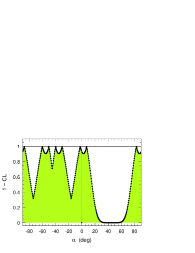
Figure 8: Fit results of the isospin analysis to the $B\rightarrow\pi\pi$ observables. Black dots: Standard Model parameterization (see Eq. (II)); shaded curve: the same but allowing arbitrary new physics contributions to the $\Delta I=1/2$ channel (see Eq. (B.2)).

Figure 8 shows the result of the frequentist fit for both parameterizations from Eqs. (II) and (B.2). As expected from the above discussion, the two curves are strictly identical except at the $\alpha=0\ [\pi]$ points where the confidence level is low in the Standard Model parameterization due to the presence of $C\!P$ violation in the data.

In contrast to the frequentist approach, the Bayesian treatment violates the equivalence described in Eq. (B.2), because choosing finite priors in one parameterization automatically restricts the phase space in the other parameterization. The Bayesian posterior PDF for $\alpha$ in the parameterization in Eq. (B.2) would yield a fairly good probability density at $\alpha\sim 0$, since the amplitudes $M_{\rm NP}$ and $\kern 1.79993pt\overline{\kern-1.79993ptM}_{\rm NP}{}$ can generate $C\!P$ violation.

It may appear legitimate to perform a fit to the $B\rightarrow\pi\pi$ data within the Standard Model, not allowing for new physics neither in the $\Delta I=3/2$ nor the $\Delta I=1/2$ transitions. From the above discussion it is not completely possible, unless amplitudes are known exactly within the Standard Model. Still it is possible within the frequentist framework to restrict the parameter space to “reasonable” ranges. Regardless of the accuracy of these ranges, this would not be the isospin analysis anymore since the isospin symmetry only predicts Eq. (II) without telling us anything about the order of magnitude of the transition amplitudes.

B.3 The RI parameterization

Mathematically, the fact that the RI parameterization leads to cataclysm in the Bayesian treatment can be understood as follows. For a given set of model parameters $T^{+-}$, $P$, $T^{00}$ in Eq. (II) one can always define the secondary parameters $\tau^{+-}$, $p$, $\tau^{00}$ such that:

$$T^{+-} = \tau^{+-}/\sin\alpha\,,$$

$$P = p-\tau^{+-}/\tan\alpha\,,$$ (16)

$$T^{00} = \tau^{00}-\tau^{+-}/\sin\alpha\,.$$

The expressions of the three amplitudes in Eq. (II) then take the form

$$A^{+-} = -i\tau^{+-}+p\,,$$

$$\sqrt{2}A^{00} = i\tau^{+-}+e^{-i\alpha}\tau^{00}-p\,,$$ (17)

$$\sqrt{2}A^{+0} = e^{-i\alpha}\tau^{00}\,,$$

where for the $C\!P$-conjugate amplitudes one has to transform $\alpha\rightarrow-\alpha$, $\tau^{+-}\rightarrow-\tau^{+-}$. It is now clear that $\tau^{+-}\neq 0$ can generate finite $C\!P$ violation even if $\alpha=0$.

The Jacobian of the transformation is

$$\left|\frac{d|\tau^{+-}|d\mathrm{Re}(p)d\mathrm{Im}(p)d\mathrm{Re}(\tau^{00})d\mathrm{Im}(\tau^{00})}{d|T^{+-}|d\mathrm{Re}(P)d\mathrm{Im}(P)d\mathrm{Re}(T^{00})d\mathrm{Im}(T^{00})}\right|=|\sin\alpha|$$ (18)

and thus, in the RI parameterization, the posterior for $\alpha$ can be written as:

$$P_{\mathrm{RI}}(\alpha)\propto{1\over\mid\sin\alpha\mid}P_{\mathrm{\mathrm{RI}_{\tau}}}(\alpha)$$ (19)

with

$$P_{\mathrm{\mathrm{RI}_{\tau}}}(\alpha) \propto \int e^{-{1\over 2}\chi^{2}\left[|\tau^{+-}|,\mathrm{Re}(p),\mathrm{Im}(p),\mathrm{Re}(\tau^{00}),\mathrm{Im}(\tau^{00}),\alpha\right]}\times$$

$$\ \ d|\tau^{+-}|d\mathrm{Re}(p)d\mathrm{Im}(p)d\mathrm{Re}(\tau^{00})d\mathrm{Im}(\tau^{00})\,.$$

The $P_{\mathrm{\mathrm{RI}_{\tau}}}$ function is the posterior PDF for $\alpha$ in the “$\mathrm{RI}_{\tau}$” parameterization. It is shown in Fig. 9 with the $B\rightarrow\pi\pi$ observables. One observes that $P_{\mathrm{\mathrm{RI}_{\tau}}}$ is regular and finite for $\alpha=0$ and $\alpha=\pi$. As a result, it follows that in the RI parameterization the posterior $P_{RI}(\alpha)$ is not only divergent at the origin (and for $\alpha=\pi$) but is an improper PDF: it cannot be normalized to unity. Applying the same treatment to the MA parameterization exhibits no singularities as the one obtained in the RI parameterization: the Jacobian $|d\mathrm{RI}_{\tau}/d\mathrm{MA}|$ behaves like $|\tau^{+-}|^{2}/\alpha$ at the origin which ensures that the posterior PDF for $\alpha$ in the MA parameterization vanishes at $\alpha=0^{\circ}$ ($\alpha=180^{\circ}$) in agreement with Fig. 2.

As an illustration of this problem, the ranges of the priors for $|T^{+-}|$, ${\rm Re}(P)$ and ${\rm Re}(T^{00})$ in Eq. (II) have been widened by a factor two compared to the ones used in Section VI. The corresponding posterior PDFs are shown in Fig. 10. One observes that the posterior PDFs are truncated and that the posterior PDF for $\alpha$ has its two peaks higher and shifted towards the endpoints ($0^{\circ}$ and $180^{\circ}$) with respect to the ones of Fig. 2. It is worth noticing that the three ranges must be extended simultaneously to detect this effect.

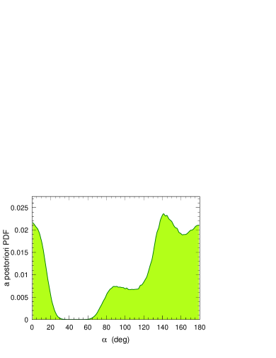
Figure 9: Posterior PDF for $\alpha$ in the “$\tau$” parametrization (see Eq. (B.3)) for $B\rightarrow\pi\pi$ decays.

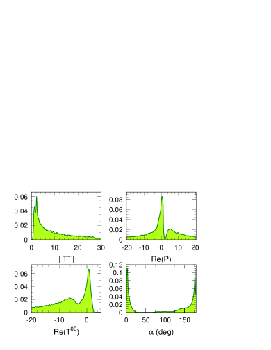
Figure 10: Posterior PDFs in the RI parameterization as obtained when widening the ranges of the priors for $|T^{+-}|$, ${\rm Re}(P)$ and ${\rm Re}(T^{00})$ by a factor two compared to the ones used in Section VI. One observes that the posterior PDFs for $|T^{+-}|$, ${\rm Re}(P)$ and ${\rm Re}(T^{00})$ do not vanish at the extremities of these extended ranges. In effect, the ranges of the prior must be extended to infinity, with the result that the posterior for $\alpha$ becomes an improper PDF, with singularities at $\alpha=0^{\circ}$ and $\alpha=180^{\circ}$.

References

- (1) J.M. Bernardo and A.F.M. Smith, Bayesian Theory, John Wiley and Sons Ltd, New York (1994); A. O’Hagan, Kendall’s Advanced Theory of Statistics, Volume 2B, Bayesian Inference, A Hodder Arnold Publication, London (1994)
- (2) D.A. Gillies, Philosophical Theories of Probability, Routledge, London (2000)
- (3) D.A. Gillies, Induction and Probability, in G.H.R. Parkinsin (ed.), An Encyclopedia of Philosophy, Chapter 9, 179-204 (1988)
- (4) R.E. Kass and L. Wasserman, The selection of prior distributions by formal rules, J. Am. Stat. Assoc. 91, 1343-1370 (1996)
- (5) D.G. Mayo, Error and the Growth of Experimental Knowledge, The University of Chicago Press, Chicago (1996)
- (6) UTfit Collaboration (M. Bona et al.), JHEP 0507, 28, (2005) [hep-ph/0501199]; http://www.utfit.org
-
(7)
The BABAR Physics Book, (P.F. Harrison and H.R. Quinn, eds.) SLAC-R-504 (1998);
http://www.slac.stanford.edu/pubs/slacreports/
slac-r-504.html - (8) M. Gronau and D. London, Phys. Rev. Lett. 65, 3381 (1990)
- (9) J. Charles, Phys. Rev. D 59, 054007 (1999) [hep-ph/9806468]
- (10) M. Pivk and F.R. Le Diberder, Eur. Phys. J. C 39, 397 (2005) [hep-ph/0406263]
- (11) CKMfitter Group (J. Charles et al.), Eur. Phys. J. C 41, 1 (2005) [hep-ph/0406184]; http://ckmfitter.in2p3.fr
- (12) Y. Grossman and H.R. Quinn, Phys. Rev. D 58, 017504 (1998) [hep-ph/9712306]; M. Gronau et al., Phys. Lett. B 514, 315 (2001) [hep-ph/0105308]
- (13) Particle Data Group (S. Eidelman et al.), Phys. Lett. B 592, 1 (2004)
- (14) R. Weatherford, Philosophical Foundations of Probability Theory, Routledge & Kegan Paul, London (1982)
- (15) M. Strevens, The Bayesian Approach to the Philosophy of Science, Macmillan Encyclopedia of Philosophy (2nd edition); http://www.strevens.org
- (16) M. Bunge, Philosophy of Physics, Reidel, Dordrecht (1973); A. Chalmers, What Is This Thing Called Science: An Assessment of the Nature and Status of Science and Its Methods, 3rd ed., Open University Press (1999)
-
(17)
F. James, A Unified Approach to Understanding Statistics,
PHYSTAT2003, SLAC (2003);
http://www.slac.stanford.edu/econf/C030908/ - (18) A. O’Hagan, Dicing with the unknown, Significance 1(3), 132 (2004)
-
(19)
F. Porter, Nucl. Inst. Meth. A 368, 793 (1996);
an extended version of the document is available at:
http://www.cithep.caltech.edu/fcp/papers/ CI_likelihoodWeb.ps -
(20)
R.D. Cousins, Comments on Methods for Setting Confidence
Limits, Workshop on Confidence Limits, CERN (2000);
http://doc.cern.ch/yellowrep/2000/2000-005/p49.pdf -
(21)
BABAR Collaboration (B. Aubert et al.),
Phys. Rev. Lett. 95, 151803 (2005) [hep-ex/0501071]; BABAR-CONF-05/13 [hep-ex/0508046] (2005);
Phys. Rev. Lett. 94, 181802 (2005) [hep-ex/0412037];
Phys. Rev. Lett. 94, 181802 (2005) [hep-ex/0412037];
Belle Collaboration (K. Abe et al.), Phys. Rev. Lett. 95, 101801 (2005) [hep-ex/0502035]; Phys. Rev. D 69, 111102 (2004) [hep-ex/0311061]; Phys. Rev. Lett. 94, 181803 (2005) [hep-ex/0408101]; Phys. Rev. D 69, 111102 (2004) [hep-ex/0311061];
CLEO Collaboration (A. Bornheim et al.), Phys. Rev. D 68, 052002 (2003) [hep-ex/0302026] -
(22)
Talk given by M. Bona [on behalf of the UTfit
Collaboration] at the workshop “Flavour in the era of LHC”, May 15-17
2006, CERN (Geneva, Switzerland);
http://mlm.home.cern.ch/mlm/FlavLHC.html -
(23)
G. Punzi, What is systematics?, CDF note Feb. 2001;
http://www-cdf.fnal.gov/physics/statistics/notes/
punzi-systdef.ps; P. Sinervo, Definition and Treatment of Systematic Uncertainties in High Energy Physics and Astrophysics, PHYSTAT2003, SLAC (2003) and references therein;
http://www.slac.stanford.edu/econf/C030908/ - (24) J. Charles, hep-ph/0606046 (2006).
- (25) T. Seidenfeld, Why I Am Not an Objective Bayesian; Some Reflections Prompted by Rosenkrantz, Theory and Decisions 11, 413-440 (1979); B. van Fraassen, Indifference: The Symmetry of Probability, Chapter 12. in Laws and symmetry (Oxford, OUP, 1989); A.P. Dawid, Invariant Prior Distributions, in S. Kotz and N.L. Johnson, Encyclopedia of Statistical Sciences (New York, Wiley, 1983), 228-36
- (26) D.R. Cox, Phystat05 conference, Oxford, England (2005); http://www.physics.ox.ac.uk/phystat05/
-
(27)
D.R. Cox and D. Mayo, Some remarks on the nature of statistical inference,
Error 2006, Virginia Tech (2006);
http://www.error06.econ.vt.edu/Cox.pdf -
(28)
BABAR Collaboration (B. Aubert et al.),
B. Lau at Rencontres de Moriond - QCD and
Hadronic Interactions at High Energy,
La Thuile, Italy (2006);
Phys. Rev. Lett. 95, 041805 (2005) [hep-ex/0503049];
Phys. Rev. Lett. 94, 131801 (2005) [hep-ex/0412067];
Phys. Rev. Lett. 93, 231801 (2004) [hep-ex/0404029]; Phys. Rev. Lett. 91, 171802 (2003) [hep-ex/0307026];
Belle Collaboration (A. Somov and A. J. Schwartz et al.), Phys. Rev. Lett. 96, 171801 (2006) [hep-ex/0601024]; Belle Collaboration (J. Zhang et al.), Phys. Rev. Lett. 91, 221801 (2003) [hep-ex/0306007] - (29) Heavy Flavour Averaging Group (E. Barberio et al.), hep-ex/0603003 (2006)
- (30) To the best of our knowledge, this reparameterization invariance was first pointed out by Helen R. Quinn at one of the BaBar workshops (1996-1997). It was later also discussed in other works: D. London, N. Sinha and R. Sinha, Phys. Rev.60 074020 (1999); F.J. Botella and J.P. Silva, Phys. Rev.71 094008 (2005); S. Baek et al., Phys. Rev.72 036004 (2005)