July 2006


SINGLE INCLUSIVE DISTRIBUTION AND TWO-PARTICLE CORRELATIONS INSIDE ONE JET

AT β€œMODIFIED LEADING LOGARITHMIC APPROXIMATION” OF QUANTUM CHROMODYNAMICS

II : STEEPEST DESCENT EVALUATION AT SMALL X𝑋\boldsymbol{X}


Redamy Perez-Ramos 111E-mail: perez@lpthe.jussieu.fr

Laboratoire de Physique ThΓ©orique et Hautes Energies 222LPTHE, tour 24-25, 5Γ¨me Γ©tage, UniversitΓ© P. et M. Curie, BP 126, 4 place Jussieu, F-75252 Paris Cedex 05 (France)

UnitΓ© Mixte de Recherche UMR 7589

UniversitΓ© Pierre et Marie Curie-Paris6; CNRS; UniversitΓ© Denis Diderot-Paris7


Abstract: The MLLA single inclusive distribution inside one high energy (gluon) jet at small xπ‘₯x is estimated by the steepest descent method. Its analytical expression is obtained outside the β€œlimiting spectrum”. It is then used to evaluate 2-particle correlations at the same level of generality. The dependence of both observables on the ratio between the infrared cutoff Q0subscript𝑄0Q_{0} and Ξ›Q​C​DsubscriptΛ𝑄𝐢𝐷\Lambda_{QCD} is studied. Fong & Webber’s results for correlations are recovered at the limits when this ratio goes to 111 and when one stays close to the peak of the single inclusive distribution.


Keywords: Perturbative Quantum Chromodynamics, Particle Correlations in jets, High Energy Colliders

1 INTRODUCTION

Exactly solving the MLLA evolution equations for the quark and gluon inclusive spectra and for 2-particle correlations inside one jet provided, at small xπ‘₯x, in [1], analytical expressions for these observables, which were unfortunately limited, for technical reasons to the β€œlimiting spectrum” λ≑ln(Q0/Ξ›Q​C​D=0\lambda\equiv\ln(Q_{0}/\Lambda_{QCD}=0. The goal of this second work is to go beyond this limit in an approximate scheme which proves very economical and powerful: the steepest descent (SD) method. It offers sizable technical progress in the calculation of both observables.

First, we perform a SD evaluation of the (quark and) gluon single inclusive distributions. Their full dependence on Ξ»πœ†\lambda is given, including the normalization. The well known shift to smaller values of xπ‘₯x of the maximum of the distribution, as compared with DLA calculations is checked, as well as its Gaussian shape around the maximum. Comparison with the results obtained numerically in [2] is done.

As shown in [1], knowing the logarithmic derivatives of the inclusive spectra immediately gives access to 2-particle correlations. This is accordingly our next step. Since, in particular, the former prove to be infra-red stable in the limit Ξ»β†’0β†’πœ†0\lambda\to 0, the result can be safely compared with the exact one obtained in [1]. The agreement turns out to be excellent, and increases with the energy scale of the process.

Last, we evaluate 2-particle correlations inside one high energy jet and study their behavior at Q0β‰ Ξ›Q​C​Dsubscript𝑄0subscriptΛ𝑄𝐢𝐷Q_{0}\neq\Lambda_{QCD}. That one recovers the results of Fong & Webber [3] close to the peak of the single inclusive distribution and when Ξ»β†’0β†’πœ†0\lambda\to 0 is an important test of the validity and efficiency of the SD method. The quantitative predictions do not substantially differ from the ones of [1] for the β€œlimiting spectrum”, which stays the best candidate to reproduce experimental results.

A conclusion summarizes the achievements, limitations and expectations of [1] and of the present work. It is completed with two technical appendices.

2 STEEPEST DESCENT EVALUATION OF THE SINGLE INCLUSIVE DISTRIBUTION

We consider the production of one hadron inside a quark or a gluon jet in a hard process. It carries the fraction xπ‘₯x of the total energy E𝐸E of the jet. Θ0subscriptΘ0\Theta_{0} is the half opening angle of the jet while ΘΘ\Theta is the angle corresponding to the first splitting with energy fraction xβ‰ͺzβ‰ͺ1much-less-thanπ‘₯𝑧much-less-than1x\ll z\ll 1.

2.1 Variables and kinematics

The variables and kinematics of the process under consideration are the same as in section 3.1 of [1].

2.2 Evolution equations for particle spectra at MLLA

We define like in [1] the logarithmic parton densities

Q​(β„“)≑x​DQ​(x),G​(β„“)=x​DG​(x)formulae-sequence𝑄ℓπ‘₯subscript𝐷𝑄π‘₯𝐺ℓπ‘₯subscript𝐷𝐺π‘₯Q(\ell)\equiv xD_{Q}(x),\qquad G(\ell)=xD_{G}(x)

for quark and gluon jets in terms of which the system of evolution equations for particle spectra at small xπ‘₯x (see eqs.Β (42) and (43) of [1]) read

Q​(β„“,y)=δ​(β„“)+CFNcβ€‹βˆ«0β„“π‘‘β„“β€²β€‹βˆ«0y𝑑y′​γ02​(β„“β€²+yβ€²)​(1βˆ’34​δ​(β„“β€²βˆ’β„“))​G​(β„“β€²,yβ€²),𝑄ℓ𝑦𝛿ℓsubscript𝐢𝐹subscript𝑁𝑐superscriptsubscript0β„“differential-dsuperscriptβ„“β€²superscriptsubscript0𝑦differential-dsuperscript𝑦′superscriptsubscript𝛾02superscriptβ„“β€²superscript𝑦′134𝛿superscriptℓ′ℓ𝐺superscriptβ„“β€²superscript𝑦′Q(\ell,y)=\delta(\ell)+\frac{C_{F}}{N_{c}}\!\!\int_{0}^{\ell}d\ell^{\prime}\int_{0}^{y}dy^{\prime}\gamma_{0}^{2}(\ell^{\prime}+y^{\prime})\Big{(}1-\frac{3}{4}\delta(\ell^{\prime}-\ell)\Big{)}G(\ell^{\prime},y^{\prime}), (1)
G​(β„“,y)=δ​(β„“)+∫0β„“π‘‘β„“β€²β€‹βˆ«0y𝑑y′​γ02​(β„“β€²+yβ€²)​(1βˆ’a​δ​(β„“β€²βˆ’β„“))​G​(β„“β€²,yβ€²),𝐺ℓ𝑦𝛿ℓsuperscriptsubscript0β„“differential-dsuperscriptβ„“β€²superscriptsubscript0𝑦differential-dsuperscript𝑦′superscriptsubscript𝛾02superscriptβ„“β€²superscript𝑦′1π‘Žπ›Ώsuperscriptℓ′ℓ𝐺superscriptβ„“β€²superscript𝑦′G(\ell,y)=\delta(\ell)+\int_{0}^{\ell}d\ell^{\prime}\int_{0}^{y}dy^{\prime}\gamma_{0}^{2}(\ell^{\prime}+y^{\prime})\Big{(}1-a\delta(\ell^{\prime}-\ell)\Big{)}G(\ell^{\prime},y^{\prime}), (2)

where

a=14​Nc​[113​Nc+43​nf​TR​(1βˆ’2​CFNc)]=nf=30.935.π‘Ž14subscript𝑁𝑐delimited-[]113subscript𝑁𝑐43subscript𝑛𝑓subscript𝑇𝑅12subscript𝐢𝐹subscript𝑁𝑐superscriptsubscript𝑛𝑓30.935a=\frac{1}{4N_{c}}\bigg{[}\frac{11}{3}N_{c}+\frac{4}{3}n_{f}T_{R}\bigg{(}\!1-\frac{2C_{F}}{N_{c}}\!\bigg{)}\bigg{]}\stackrel{{\scriptstyle n_{f}=3}}{{=}}0.935. (3)

The terms ∝34proportional-toabsent34\propto\frac{3}{4} in (1) and ∝aproportional-toabsentπ‘Ž\propto a in (2) account for hard corrections to soft gluon multiplication, sub-leading gβ†’q​qΒ―β†’π‘”π‘žΒ―π‘žg\!\to\!q\bar{q} splittings, strict angular ordering and energy conservation.

2.3 Evolution equations; steepest descent evaluation

The exact solution of (2) is demonstrated in [1] to be given by the Mellin’s integral representation

G​(β„“,y)𝐺ℓ𝑦\displaystyle G\left(\ell,y\right) =\displaystyle= (β„“+y+Ξ»)β€‹βˆ¬d​ω​d​ν(2​π​i)2​eω​ℓ+ν​yβ€‹βˆ«0∞d​sΞ½+s​(ω​(Ξ½+s)(Ο‰+s)​ν)1/β​(Ο‰βˆ’Ξ½)​(Ξ½Ξ½+s)a/β​eβˆ’Ξ»β€‹sβ„“π‘¦πœ†double-integralπ‘‘πœ”π‘‘πœˆsuperscript2πœ‹π‘–2superscriptπ‘’πœ”β„“πœˆπ‘¦superscriptsubscript0π‘‘π‘ πœˆπ‘ superscriptπœ”πœˆπ‘ πœ”π‘ πœˆ1π›½πœ”πœˆsuperscriptπœˆπœˆπ‘ π‘Žπ›½superscriptπ‘’πœ†π‘ \displaystyle\left(\ell\!+\!y\!+\!\lambda\right)\!\!\iint\frac{d\omega\,d\nu}{\left(2\pi i\right)^{2}}e^{\omega\ell+\nu y}\!\!\int_{0}^{\infty}\frac{ds}{\nu+s}\!\!\left(\!\frac{\omega\left(\nu+s\right)}{\left(\omega+s\right)\nu}\!\right)^{1/\beta\left(\omega-\nu\right)}\!\!\left(\!\frac{\nu}{\nu+s}\!\right)^{a/\beta}\,e^{-\lambda s} (4)
=\displaystyle= (β„“+y+Ξ»)β€‹βˆ¬d​ω​d​ν(2​π​i)2​eω​ℓ+ν​yβ€‹βˆ«0∞d​sΞ½+s​(Ξ½Ξ½+s)a/β​eσ​(s),β„“π‘¦πœ†double-integralπ‘‘πœ”π‘‘πœˆsuperscript2πœ‹π‘–2superscriptπ‘’πœ”β„“πœˆπ‘¦superscriptsubscript0π‘‘π‘ πœˆπ‘ superscriptπœˆπœˆπ‘ π‘Žπ›½superscriptπ‘’πœŽπ‘ \displaystyle\left(\ell\!+\!y\!+\!\lambda\right)\!\!\iint\frac{d\omega\,d\nu}{\left(2\pi i\right)^{2}}e^{\omega\ell+\nu y}\!\!\int_{0}^{\infty}\frac{ds}{\nu+s}\left(\!\frac{\nu}{\nu+s}\!\right)^{a/\beta}e^{\sigma(s)}, (5)

where we have exponentiated the kernel (symmetrical in (Ο‰,Ξ½)πœ”πœˆ(\omega,\nu))

σ​(s)=1β​(Ο‰βˆ’Ξ½)​ln⁑(ω​(Ξ½+s)ν​(Ο‰+s))βˆ’Ξ»β€‹s.πœŽπ‘ 1π›½πœ”πœˆπœ”πœˆπ‘ πœˆπœ”π‘ πœ†π‘ \sigma(s)=\frac{1}{\beta(\omega-\nu)}\ln\left(\!\frac{\omega(\nu+s)}{\nu(\omega+s)}\!\right)-\lambda s. (6)

(4) will be estimated by the SD method. The value s0subscript𝑠0s_{0} of the saddle point, satisfying d​σ​(s)d​s|s=s0=0evaluated-atπ‘‘πœŽπ‘ π‘‘π‘ π‘ subscript𝑠00\frac{d\sigma(s)}{ds}\Big{|}_{s=s_{0}}=0, reads (see [7])

s0​(Ο‰,Ξ½)=12​[4β​λ+(Ο‰βˆ’Ξ½)2βˆ’(Ο‰+Ξ½)].subscript𝑠0πœ”πœˆ12delimited-[]4π›½πœ†superscriptπœ”πœˆ2πœ”πœˆs_{0}(\omega,\nu)=\frac{1}{2}\left[\sqrt{\frac{4}{\beta\lambda}+(\omega-\nu)^{2}}-(\omega+\nu)\right]. (7)

One makes a Taylor expansion of σ​(s)πœŽπ‘ \sigma(s) nearby s0subscript𝑠0s_{0}:

σ​(s)=σ​(s0)+12​σ′′​(s0)​(sβˆ’s0)2+π’ͺ​((sβˆ’s0)2),σ′′​(s0)=βˆ’Ξ²β€‹Ξ»2​4β​λ+(Ο‰βˆ’Ξ½)2<0,formulae-sequenceπœŽπ‘ πœŽsubscript𝑠012superscriptπœŽβ€²β€²subscript𝑠0superscript𝑠subscript𝑠02π’ͺsuperscript𝑠subscript𝑠02superscriptπœŽβ€²β€²subscript𝑠0𝛽superscriptπœ†24π›½πœ†superscriptπœ”πœˆ20\sigma(s)=\sigma(s_{0})+\frac{1}{2}\sigma^{\prime\prime}(s_{0})(s-s_{0})^{2}+{\cal O}\left((s-s_{0})^{2}\right),\quad\sigma^{\prime\prime}(s_{0})=-\beta\lambda^{2}\sqrt{\frac{4}{\beta\lambda}+(\omega-\nu)^{2}}<0, (8)

such that

∫0∞d​sΞ½+s​(ω​(Ξ½+s)(Ο‰+s)​ν)1/β​(Ο‰βˆ’Ξ½)​(Ξ½Ξ½+s)a/β​eβˆ’Ξ»β€‹ssuperscriptsubscript0π‘‘π‘ πœˆπ‘ superscriptπœ”πœˆπ‘ πœ”π‘ πœˆ1π›½πœ”πœˆsuperscriptπœˆπœˆπ‘ π‘Žπ›½superscriptπ‘’πœ†π‘ \displaystyle\int_{0}^{\infty}\frac{ds}{\nu+s}\!\!\left(\!\frac{\omega\left(\nu+s\right)}{\left(\omega+s\right)\nu}\!\right)^{1/\beta\left(\omega-\nu\right)}\!\!\left(\!\frac{\nu}{\nu+s}\!\right)^{a/\beta}\,e^{-\lambda s}\!\! β‰ˆΞ»β‰«1superscriptmuch-greater-thanπœ†1\displaystyle\!\!\stackrel{{\scriptstyle\lambda\gg 1}}{{\approx}}\!\! 2​π2​eσ​(s0)(Ξ½+s0)β€‹βˆ£Οƒβ€²β€²β€‹(s0)βˆ£β€‹(Ξ½Ξ½+s0)a/Ξ².2πœ‹2superscriptπ‘’πœŽsubscript𝑠0𝜈subscript𝑠0delimited-∣∣superscriptπœŽβ€²β€²subscript𝑠0superscript𝜈𝜈subscript𝑠0π‘Žπ›½\displaystyle\!\!2\sqrt{\frac{\pi}{2}}\displaystyle{\frac{e^{\sigma(s_{0})}}{(\nu+s_{0})\sqrt{\mid\!\sigma^{\prime\prime}(s_{0})\!\mid}}}\left(\!\frac{\nu}{\nu+s_{0}}\!\right)^{a/\beta}\!\!. (9)

The condition λ≫1much-greater-thanπœ†1\lambda\!\gg\!1β‡’β‡’\RightarrowΞ±s/Ο€β‰ͺ1much-less-thansubscriptπ›Όπ‘ πœ‹1\alpha_{s}/\pi\!\ll\!1 333in (8), Ξ»πœ†\lambda appears to the power 3/2>13213/2>1, which guarantees the fast convergence of the SD as Ξ»πœ†\lambda increases. guarantees, in particular, the convergence of the perturbative approach. Substituting (9) in (4) yields

G​(β„“,y)β‰ˆ2​π2​(β„“+y+Ξ»)β€‹βˆ¬d​ω​d​ν(2​π​i)2​eϕ​(Ο‰,Ξ½,β„“,y)(Ξ½+s0)β€‹βˆ£Οƒβ€²β€²β€‹(s0)βˆ£β€‹(Ξ½Ξ½+s0)a/Ξ²,𝐺ℓ𝑦2πœ‹2β„“π‘¦πœ†double-integralπ‘‘πœ”π‘‘πœˆsuperscript2πœ‹π‘–2superscript𝑒italic-Ο•πœ”πœˆβ„“π‘¦πœˆsubscript𝑠0delimited-∣∣superscriptπœŽβ€²β€²subscript𝑠0superscript𝜈𝜈subscript𝑠0π‘Žπ›½G\left(\ell,y\right)\approx 2\sqrt{\frac{\pi}{2}}(\ell+y+\lambda)\iint\frac{d\omega\,d\nu}{\left(2\pi i\right)^{2}}\,\displaystyle{\frac{e^{\phi\left(\omega,\nu,\ell,y\right)}}{(\nu+s_{0})\sqrt{\mid\!\sigma^{\prime\prime}(s_{0})\!\mid}}}\left(\!\frac{\nu}{\nu+s_{0}}\!\right)^{a/\beta}, (10)

where the argument of the exponential is

ϕ​(Ο‰,Ξ½,β„“,y)=ω​ℓ+ν​y+1β​(Ο‰βˆ’Ξ½)​ln⁑ω​(Ξ½+s0)(Ο‰+s0)β€‹Ξ½βˆ’Ξ»β€‹s0.italic-Ο•πœ”πœˆβ„“π‘¦πœ”β„“πœˆπ‘¦1π›½πœ”πœˆπœ”πœˆsubscript𝑠0πœ”subscript𝑠0πœˆπœ†subscript𝑠0\phi\left(\omega,\nu,\ell,y\right)=\omega\ell+\nu y+\frac{1}{\beta\left(\omega-\nu\right)}\ln{\frac{\omega\left(\nu+s_{0}\right)}{\left(\omega+s_{0}\right)\nu}}-\lambda s_{0}. (11)

Once again, we perform the SD method to evaluate (10). The saddle point (Ο‰0,Ξ½0)subscriptπœ”0subscript𝜈0(\omega_{0},\nu_{0}) satisfies the equations

βˆ‚Ο•βˆ‚Ο‰=β„“βˆ’1β​(Ο‰βˆ’Ξ½)2​ln⁑ω​(Ξ½+s0)(Ο‰+s0)​ν+1β​ω​(Ο‰βˆ’Ξ½)βˆ’Ξ»β€‹(Ξ½+s0)(Ο‰βˆ’Ξ½)=0,italic-Ο•πœ”β„“1𝛽superscriptπœ”πœˆ2πœ”πœˆsubscript𝑠0πœ”subscript𝑠0𝜈1π›½πœ”πœ”πœˆπœ†πœˆsubscript𝑠0πœ”πœˆ0\frac{\partial\phi}{\partial\omega}=\ell-\frac{1}{\beta\left(\omega-\nu\right)^{2}}\ln{\frac{\omega\left(\nu+s_{0}\right)}{\left(\omega+s_{0}\right)\nu}}+\frac{1}{\beta\omega\left(\omega-\nu\right)}-\lambda\frac{\left(\nu+s_{0}\right)}{\left(\omega-\nu\right)}=0, (12a)
βˆ‚Ο•βˆ‚Ξ½=y+1β​(Ο‰βˆ’Ξ½)2​ln⁑ω​(Ξ½+s0)(Ο‰+s0)β€‹Ξ½βˆ’1β​ν​(Ο‰βˆ’Ξ½)+λ​(Ο‰+s0)(Ο‰βˆ’Ξ½)=0.italic-Ο•πœˆπ‘¦1𝛽superscriptπœ”πœˆ2πœ”πœˆsubscript𝑠0πœ”subscript𝑠0𝜈1π›½πœˆπœ”πœˆπœ†πœ”subscript𝑠0πœ”πœˆ0\frac{\partial\phi}{\partial\nu}=y+\frac{1}{\beta\left(\omega-\nu\right)^{2}}\ln{\frac{\omega\left(\nu+s_{0}\right)}{\left(\omega+s_{0}\right)\nu}}-\frac{1}{\beta\nu\left(\omega-\nu\right)}+\lambda\frac{\left(\omega+s_{0}\right)}{\left(\omega-\nu\right)}=0. (12b)

Adding and subtracting (12a) and (12b) gives respectively

Ο‰0​ν0=1β​(β„“+y+Ξ»),subscriptπœ”0subscript𝜈01π›½β„“π‘¦πœ†\omega_{0}\nu_{0}=\frac{1}{\beta\left(\ell+y+\lambda\right)}, (13a)
yβˆ’β„“=1β​(Ο‰0βˆ’Ξ½0)​(1Ο‰0+1Ξ½0)βˆ’2β​(Ο‰0βˆ’Ξ½0)2​ln⁑ω0​(Ξ½0+s0)(Ο‰0+s0)​ν0βˆ’Ξ»β€‹Ο‰0+Ξ½0+2​s0Ο‰0βˆ’Ξ½0;𝑦ℓ1𝛽subscriptπœ”0subscript𝜈01subscriptπœ”01subscript𝜈02𝛽superscriptsubscriptπœ”0subscript𝜈02subscriptπœ”0subscript𝜈0subscript𝑠0subscriptπœ”0subscript𝑠0subscript𝜈0πœ†subscriptπœ”0subscript𝜈02subscript𝑠0subscriptπœ”0subscript𝜈0y-\ell=\frac{1}{\beta\left(\omega_{0}-\nu_{0}\right)}\left(\frac{1}{\omega_{0}}+\frac{1}{\nu_{0}}\right)-\frac{2}{\beta\left(\omega_{0}-\nu_{0}\right)^{2}}\ln{\frac{\omega_{0}\left(\nu_{0}+s_{0}\right)}{\left(\omega_{0}+s_{0}\right)\nu_{0}}}-\lambda\frac{\omega_{0}+\nu_{0}+2s_{0}}{\omega_{0}-\nu_{0}}; (13b)

(Ο‰0,Ξ½0)subscriptπœ”0subscript𝜈0(\omega_{0},\nu_{0}) also satisfies (from (7))

(Ο‰0+s0)​(Ξ½0+s0)=1β​λ.subscriptπœ”0subscript𝑠0subscript𝜈0subscript𝑠01π›½πœ†\left(\omega_{0}+s_{0}\right)\left(\nu_{0}+s_{0}\right)=\frac{1}{\beta\lambda}. (14)

One can substitute the expressions (12a) and (12b) of β„“β„“\ell and y𝑦y into (11), which yields

φ≑ϕ​(Ο‰0,Ξ½0,β„“,y)=2β​(Ο‰0βˆ’Ξ½0)​ln⁑ω0​(Ξ½0+s0)(Ο‰0+s0)​ν0.πœ‘italic-Ο•subscriptπœ”0subscript𝜈0ℓ𝑦2𝛽subscriptπœ”0subscript𝜈0subscriptπœ”0subscript𝜈0subscript𝑠0subscriptπœ”0subscript𝑠0subscript𝜈0\ \varphi\equiv\phi(\omega_{0},\nu_{0},\ell,y)=\frac{2}{\beta\left(\omega_{0}-\nu_{0}\right)}\ln{\frac{\omega_{0}\left(\nu_{0}+s_{0}\right)}{\left(\omega_{0}+s_{0}\right)\nu_{0}}}. (15)

Introducing the variables (ΞΌ,Ο…)πœ‡πœ(\mu,\upsilon) [7] to parametrize (Ο‰0,Ξ½0)subscriptπœ”0subscript𝜈0(\omega_{0},\nu_{0}) through

Ο‰0​(Ξ½0)=1β​(β„“+y+Ξ»)​e±μ​(β„“,y),(Ο‰0+s0)​(Ξ½0+s0)=1β​λ​e±υ​(β„“,y),formulae-sequencesubscriptπœ”0subscript𝜈01π›½β„“π‘¦πœ†superscript𝑒plus-or-minusπœ‡β„“π‘¦subscriptπœ”0subscript𝑠0subscript𝜈0subscript𝑠01π›½πœ†superscript𝑒plus-or-minusπœβ„“π‘¦\omega_{0}\left(\nu_{0}\right)=\frac{1}{\sqrt{\beta(\ell\!+\!y\!+\!\lambda)}}e^{\pm\mu(\ell,y)},\qquad\left(\omega_{0}+s_{0}\right)\left(\nu_{0}+s_{0}\right)=\frac{1}{\sqrt{\beta\lambda}}e^{\pm\upsilon(\ell,y)}, (16)

one rewrites (15) and (13b) respectively in the form

φ​(ΞΌ,Ο…)=2β​(β„“+y+Ξ»βˆ’Ξ»)β€‹ΞΌβˆ’Ο…sinhβ‘ΞΌβˆ’sinh⁑υ,πœ‘πœ‡πœ2π›½β„“π‘¦πœ†πœ†πœ‡πœπœ‡πœ\varphi(\mu,\upsilon)=\frac{2}{\sqrt{\beta}}\left(\sqrt{\ell+y+\lambda}-\sqrt{\lambda}\right)\,\frac{\mu-\upsilon}{\sinh\mu-\sinh\upsilon}, (17)
yβˆ’β„“y+β„“=(sinh⁑2β€‹ΞΌβˆ’2​μ)βˆ’(sinh⁑2β€‹Ο…βˆ’2​υ)2​(sinh2β‘ΞΌβˆ’sinh2⁑υ);𝑦ℓ𝑦ℓ2πœ‡2πœ‡2𝜐2𝜐2superscript2πœ‡superscript2𝜐\frac{y-\ell}{y+\ell}=\frac{\left(\sinh 2\mu-2\mu\right)-\left(\sinh 2\upsilon-2\upsilon\right)}{2\left(\sinh^{2}\mu-\sinh^{2}\upsilon\right)}; (18a)

moreover, since Ο‰0βˆ’Ξ½0=(Ο‰0βˆ’s0)βˆ’(Ξ½0βˆ’s0)subscriptπœ”0subscript𝜈0subscriptπœ”0subscript𝑠0subscript𝜈0subscript𝑠0\omega_{0}-\nu_{0}=(\omega_{0}-s_{0})-(\nu_{0}-s_{0}), (ΞΌ,Ο…)πœ‡πœ(\mu,\upsilon) also satisfy

sinh⁑υλ=sinh⁑μℓ+y+Ξ».πœπœ†πœ‡β„“π‘¦πœ†\frac{\sinh\upsilon}{\sqrt{\lambda}}=\frac{\sinh\mu}{\sqrt{\ell+y+\lambda}}. (18b)

Performing a Taylor expansion of ϕ​(Ο‰,Ξ½,β„“,y)italic-Ο•πœ”πœˆβ„“π‘¦\phi(\omega,\nu,\ell,y) around (Ο‰0,Ξ½0)subscriptπœ”0subscript𝜈0(\omega_{0},\nu_{0}), which needs evaluating βˆ‚2Ο•βˆ‚Ο‰2superscript2italic-Ο•superscriptπœ”2\frac{\partial^{2}\phi}{\partial\omega^{2}}, βˆ‚2Ο•βˆ‚Ξ½2superscript2italic-Ο•superscript𝜈2\frac{\partial^{2}\phi}{\partial\nu^{2}} and βˆ‚2Ο•βˆ‚Ο‰β€‹βˆ‚Ξ½superscript2italic-Ο•πœ”πœˆ\frac{\partial^{2}\phi}{\partial\omega\partial\nu} (see appendix A.1), treating (Y+Ξ»)π‘Œπœ†(Y+\lambda) as a large parameter and making use of (16) provides the SD result

G​(β„“,y)β‰ˆπ’©β€‹(ΞΌ,Ο…,Ξ»)​exp⁑[2β​(β„“+y+Ξ»βˆ’Ξ»)β€‹ΞΌβˆ’Ο…sinhβ‘ΞΌβˆ’sinh⁑υ+Ο…βˆ’aβ​(ΞΌβˆ’Ο…)],πΊβ„“π‘¦π’©πœ‡πœπœ†2π›½β„“π‘¦πœ†πœ†πœ‡πœπœ‡πœπœπ‘Žπ›½πœ‡πœ\displaystyle G(\ell,y)\approx{\cal N}(\mu,\upsilon,\lambda)\exp\Big{[}\frac{2}{\sqrt{\beta}}\left(\sqrt{\ell+y+\lambda}-\sqrt{\lambda}\right)\frac{\mu-\upsilon}{\sinh\mu-\sinh\upsilon}+\upsilon-\frac{a}{\beta}(\mu-\upsilon)\Big{]}, (19)

where

𝒩​(ΞΌ,Ο…,Ξ»)=12​(β„“+y+Ξ»)​(Ξ²Ξ»)1/4π​cosh⁑υ​D​e​t​A​(ΞΌ,Ο…)​(Ξ»β„“+y+Ξ»)a/2β€‹Ξ²π’©πœ‡πœπœ†12β„“π‘¦πœ†superscriptπ›½πœ†14πœ‹πœπ·π‘’π‘‘π΄πœ‡πœsuperscriptπœ†β„“π‘¦πœ†π‘Ž2𝛽{\cal N}(\mu,\upsilon,\lambda)=\frac{1}{2}(\ell\!+\!y\!+\!\lambda)\frac{\left(\frac{\beta}{\lambda}\right)^{1/4}}{\sqrt{\pi\cosh\upsilon\,DetA(\mu,\upsilon)}}\left(\frac{\lambda}{\ell+y+\lambda}\right)^{a/2\beta}

with (see details in appendix A.1)

D​e​t​A​(ΞΌ,Ξ½)=β​(β„“+y+Ξ»)3​[(ΞΌβˆ’Ο…)​cosh⁑μ​cosh⁑υ+cosh⁑μ​sinhβ‘Ο…βˆ’sinh⁑μ​cosh⁑υsinh3⁑μ​cosh⁑υ].π·π‘’π‘‘π΄πœ‡πœˆπ›½superscriptβ„“π‘¦πœ†3delimited-[]πœ‡πœπœ‡πœπœ‡πœπœ‡πœsuperscript3πœ‡πœDetA(\mu,\nu)=\beta\,(\ell\!+\!y\!+\!\lambda)^{3}\left[\frac{(\mu\!-\!\upsilon)\cosh\mu\cosh\upsilon\!+\!\cosh\mu\sinh\upsilon\!-\!\sinh\mu\cosh\upsilon}{\sinh^{3}\mu\cosh\upsilon}\right]. (20)

2.3.1 Shape of the spectrum given in eq.Β (19)

We normalize (19) by the MLLA mean multiplicity inside one jet [8]

n¯​(Y)β‰ˆΞ»β‰«112​(Y+λλ)βˆ’12​aΞ²+14​exp⁑[2β​(Y+Ξ»βˆ’Ξ»)].superscriptmuch-greater-thanπœ†1Β―π‘›π‘Œ12superscriptπ‘Œπœ†πœ†12π‘Žπ›½142π›½π‘Œπœ†πœ†\bar{n}(Y)\stackrel{{\scriptstyle\lambda\gg 1}}{{\approx}}\frac{1}{2}\left(\frac{Y+\lambda}{\lambda}\right)^{\displaystyle{-\frac{1}{2}\frac{a}{\beta}+\frac{1}{4}}}\exp\left[\frac{2}{\sqrt{\beta}}\left(\sqrt{Y+\lambda}-\sqrt{\lambda}\right)\right].

The normalized expression for the single inclusive distribution as a function of β„“=ln⁑(1/x)β„“1π‘₯\ell=\ln(1/x) is accordingly obtained by setting y=Yβˆ’β„“π‘¦π‘Œβ„“y=Y-\ell in (19)

G​(β„“,Y)n¯​(Y)β‰ˆΞ²1/2​(Y+Ξ»)3/2π​cosh⁑υ​D​e​t​A​(ΞΌ,Ο…)​exp⁑[2β​(Y+Ξ»βˆ’Ξ»)​(ΞΌβˆ’Ο…sinhβ‘ΞΌβˆ’sinhβ‘Ο…βˆ’1)+Ο…βˆ’aβ​(ΞΌβˆ’Ο…)].πΊβ„“π‘ŒΒ―π‘›π‘Œsuperscript𝛽12superscriptπ‘Œπœ†32πœ‹πœπ·π‘’π‘‘π΄πœ‡πœ2π›½π‘Œπœ†πœ†πœ‡πœπœ‡πœ1πœπ‘Žπ›½πœ‡πœ\displaystyle\frac{G(\ell,Y)}{\bar{n}(Y)}\approx\sqrt{\frac{\beta^{1/2}(Y\!+\!\lambda)^{3/2}}{\pi\cosh\upsilon DetA(\mu,\upsilon)}}\!\exp\!\Big{[}\frac{2}{\sqrt{\beta}}\left(\sqrt{Y\!+\!\lambda}\!-\!\sqrt{\lambda}\right)\!\left(\frac{\mu\!-\!\upsilon}{\sinh\mu\!-\!\sinh\upsilon}\!-\!1\right)\!+\!\upsilon\!-\!\frac{a}{\beta}(\mu\!-\!\upsilon)\Big{]}. (21)

One can explicitly verify that (21) preserves the position of the maximum [8][9][10] at

β„“m​a​x=Y2+12​aβ​(Y+Ξ»βˆ’Ξ»)>Y2,subscriptβ„“π‘šπ‘Žπ‘₯π‘Œ212π‘Žπ›½π‘Œπœ†πœ†π‘Œ2\ell_{max}=\frac{Y}{2}+\frac{1}{2}\frac{a}{\beta}\left(\sqrt{Y+\lambda}-\sqrt{\lambda}\right)>\frac{Y}{2}, (22)

as well as the gaussian shape of the distribution around (22) (see appendix A.2)

G​(β„“,Y)n¯​(Y)β‰ˆ(3π​β​[(Y+Ξ»)3/2βˆ’Ξ»3/2])1/2​exp⁑(βˆ’2β​3(Y+Ξ»)3/2βˆ’Ξ»3/2​(β„“βˆ’β„“m​a​x)22).πΊβ„“π‘ŒΒ―π‘›π‘Œsuperscript3πœ‹π›½delimited-[]superscriptπ‘Œπœ†32superscriptπœ†32122𝛽3superscriptπ‘Œπœ†32superscriptπœ†32superscriptβ„“subscriptβ„“π‘šπ‘Žπ‘₯22\frac{G(\ell,Y)}{\bar{n}(Y)}\approx\left(\frac{3}{\pi\sqrt{\beta}\left[(Y+\lambda)^{3/2}-\lambda^{3/2}\right]}\right)^{1/2}\!\!\exp\left(-\frac{2}{\sqrt{\beta}}\,\frac{3}{(Y+\lambda)^{3/2}-\lambda^{3/2}}\frac{\left(\ell-\ell_{max}\right)^{2}}{2}\right). (23)

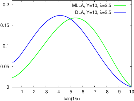
In Fig.1 we compare for Y=10π‘Œ10Y=10 and Ξ»=2.5πœ†2.5\lambda=2.5 the MLLA curve with DLA (by setting a=0π‘Ž0a=0 in (21)). The general features of the MLLA curve (21) at Ξ»β‰ 0πœ†0\lambda\neq 0 are in good agreement with those of [2].
Refer to caption
Figure 1: SD normalized spectrum: DLA (blue), MLLA (green); Y=10.0π‘Œ10.0Y=10.0, Ξ»=2.5πœ†2.5\lambda=2.5.

The shape of the single inclusive spectrum given by (21) can easily be proved to be β€œinfrared stable” (it has indeed a final limit when Ξ»β†’0β†’πœ†0\lambda\to 0).

2.4 Logarithmic derivatives

Their calculation is important since they appear in the expressions of 2-particle correlations.

Exponentiating the (β„“,y)ℓ𝑦(\ell,y) dependence of the factor 𝒩𝒩{\cal N} in (19), we decompose the whole expression in two pieces

ψ=Ο†+Ξ΄β€‹Οˆ,πœ“πœ‘π›Ώπœ“\psi=\varphi+\delta\psi, (24)

where Ο†πœ‘\varphi, given in (17), is the DLA term for the shape of the distribution [7], and

Ξ΄β€‹Οˆ=βˆ’12​(1+aΞ²)​ln⁑(β„“+y+Ξ»)βˆ’aβ​μ+(1+aΞ²)​υ+12​ln⁑[Q​(ΞΌ,Ο…)]π›Ώπœ“121π‘Žπ›½β„“π‘¦πœ†π‘Žπ›½πœ‡1π‘Žπ›½πœ12π‘„πœ‡πœ\delta\psi=-\frac{1}{2}\left(1+\frac{a}{\beta}\right)\ln(\ell+y+\lambda)-\frac{a}{\beta}\mu+\left(1+\frac{a}{\beta}\right)\upsilon+\frac{1}{2}\ln[Q(\mu,\upsilon)] (25)

is the sub-leading contribution (in the sense that its derivative gives the MLLA correction), where

Q​(ΞΌ,Ο…)≑β​(β„“+y+Ξ»)3cosh⁑υ​D​e​t​A​(ΞΌ,Ο…)=sinh3⁑μ(ΞΌβˆ’Ο…)​cosh⁑μ​cosh⁑υ+cosh⁑μ​sinhβ‘Ο…βˆ’sinh⁑μ​cosh⁑υ.π‘„πœ‡πœπ›½superscriptβ„“π‘¦πœ†3πœπ·π‘’π‘‘π΄πœ‡πœsuperscript3πœ‡πœ‡πœπœ‡πœπœ‡πœπœ‡πœQ(\mu,\upsilon)\equiv\frac{\beta(\ell+y+\lambda)^{3}}{\cosh\upsilon Det\,A(\mu,\upsilon)}=\frac{\sinh^{3}\mu}{(\mu\!-\!\upsilon)\cosh\mu\cosh\upsilon\!+\!\cosh\mu\sinh\upsilon\!-\!\sinh\mu\cosh\upsilon}.

By the definition of the saddle point, the derivatives of (17) over β„“β„“\ell and y𝑦y respectively read:

Ο†β„“=Ο‰0=Ξ³0​eΞΌ,Ο†y=Ξ½0=Ξ³0​eβˆ’ΞΌ.formulae-sequencesubscriptπœ‘β„“subscriptπœ”0subscript𝛾0superscriptπ‘’πœ‡subscriptπœ‘π‘¦subscript𝜈0subscript𝛾0superscriptπ‘’πœ‡\varphi_{\ell}=\omega_{0}=\gamma_{0}e^{\mu},\qquad\qquad\varphi_{y}=\nu_{0}=\gamma_{0}e^{-\mu}. (26)

We introduce (see appendix A.3)

ℒ​(ΞΌ,Ο…)=βˆ’aΞ²+L​(ΞΌ,Ο…),L​(ΞΌ,Ο…)=12β€‹βˆ‚βˆ‚ΞΌβ€‹ln⁑[Q​(ΞΌ,Ο…)],formulae-sequenceβ„’πœ‡πœπ‘Žπ›½πΏπœ‡πœπΏπœ‡πœ12πœ‡π‘„πœ‡πœ\displaystyle{\cal{L}}(\mu,\upsilon)=-\frac{a}{\beta}+L(\mu,\upsilon),\qquad\quad L(\mu,\upsilon)=\frac{1}{2}\frac{\partial}{\partial\mu}\ln[Q(\mu,\upsilon)], (27)
(28)
(29)
𝒦​(ΞΌ,Ο…)=1+aΞ²+K​(ΞΌ,Ο…),K​(ΞΌ,Ο…)=12β€‹βˆ‚βˆ‚Ο…β€‹ln⁑[Q​(ΞΌ,Ο…)]formulae-sequenceπ’¦πœ‡πœ1π‘Žπ›½πΎπœ‡πœπΎπœ‡πœ12πœπ‘„πœ‡πœ\displaystyle{\cal{K}}(\mu,\upsilon)=1+\frac{a}{\beta}+K(\mu,\upsilon),\qquad\quad K(\mu,\upsilon)=\frac{1}{2}\frac{\partial}{\partial\upsilon}\ln[Q(\mu,\upsilon)] (30)

and make use of

βˆ‚Ο…βˆ‚β„“=tanh⁑υ​(cothβ‘ΞΌβ€‹βˆ‚ΞΌβˆ‚β„“βˆ’12​β​γ02),βˆ‚Ο…βˆ‚y=tanh⁑υ​(cothβ‘ΞΌβ€‹βˆ‚ΞΌβˆ‚yβˆ’12​β​γ02),formulae-sequenceπœβ„“πœhyperbolic-cotangentπœ‡πœ‡β„“12𝛽superscriptsubscript𝛾02πœπ‘¦πœhyperbolic-cotangentπœ‡πœ‡π‘¦12𝛽superscriptsubscript𝛾02\frac{\partial\upsilon}{\partial\ell}=\tanh\upsilon\left(\coth\mu\frac{\partial\mu}{\partial\ell}-\frac{1}{2}\beta\gamma_{0}^{2}\right),\qquad\quad\frac{\partial\upsilon}{\partial y}=\tanh\upsilon\left(\coth\mu\frac{\partial\mu}{\partial y}-\frac{1}{2}\beta\gamma_{0}^{2}\right),

that follows from (18b), to write Ξ΄β€‹Οˆβ„“,Ξ΄β€‹Οˆy𝛿subscriptπœ“β„“π›Ώsubscriptπœ“π‘¦\delta\psi_{\ell},\,\,\delta\psi_{y} in terms of βˆ‚ΞΌβˆ‚β„“πœ‡β„“\frac{\partial\mu}{\partial\ell}, βˆ‚ΞΌβˆ‚yπœ‡π‘¦\frac{\partial\mu}{\partial y}

Ξ΄β€‹Οˆβ„“=βˆ’12​(1+aΞ²+tanh⁑υ​𝒦​(ΞΌ,Ο…))​β​γ02+(ℒ​(ΞΌ,Ο…)+tanh⁑υ​coth⁑μ​𝒦​(ΞΌ,Ο…))β€‹βˆ‚ΞΌβˆ‚β„“,𝛿subscriptπœ“β„“121π‘Žπ›½πœπ’¦πœ‡πœπ›½superscriptsubscript𝛾02β„’πœ‡πœπœhyperbolic-cotangentπœ‡π’¦πœ‡πœπœ‡β„“\displaystyle\hskip-14.22636pt\delta\psi_{\ell}=-\frac{1}{2}\left(1+\frac{a}{\beta}+\tanh\upsilon\,{\cal{K}}(\mu,\upsilon)\right)\beta\gamma_{0}^{2}+\bigg{(}{\cal{L}}(\mu,\upsilon)+\tanh{\upsilon}\coth{\mu}\,{\cal{K}}(\mu,\upsilon)\bigg{)}\frac{\partial\mu}{\partial\ell}, (31a)
Ξ΄β€‹Οˆy=βˆ’12​(1+aΞ²+tanh⁑υ​𝒦​(ΞΌ,Ο…))​β​γ02+(ℒ​(ΞΌ,Ο…)+tanh⁑υ​coth⁑μ​𝒦​(ΞΌ,Ο…))β€‹βˆ‚ΞΌβˆ‚y.𝛿subscriptπœ“π‘¦121π‘Žπ›½πœπ’¦πœ‡πœπ›½superscriptsubscript𝛾02β„’πœ‡πœπœhyperbolic-cotangentπœ‡π’¦πœ‡πœπœ‡π‘¦\displaystyle\hskip-14.22636pt\delta\psi_{y}=-\frac{1}{2}\left(1+\frac{a}{\beta}+\tanh\upsilon\,{\cal{K}}(\mu,\upsilon)\right)\beta\gamma_{0}^{2}+\bigg{(}{\cal{L}}(\mu,\upsilon)+\tanh{\upsilon}\coth{\mu}\,{\cal{K}}(\mu,\upsilon)\bigg{)}\frac{\partial\mu}{\partial y}. (31b)

Using (18a) and (18b) we obtain

βˆ‚ΞΌβˆ‚β„“=βˆ’12​β​γ02​[1+eμ​Q~​(ΞΌ,Ο…)],βˆ‚ΞΌβˆ‚y=12​β​γ02​[1+eβˆ’ΞΌβ€‹Q~​(ΞΌ,Ο…)]formulae-sequenceπœ‡β„“12𝛽superscriptsubscript𝛾02delimited-[]1superscriptπ‘’πœ‡~π‘„πœ‡πœπœ‡π‘¦12𝛽superscriptsubscript𝛾02delimited-[]1superscriptπ‘’πœ‡~π‘„πœ‡πœ\frac{\partial\mu}{\partial\ell}=-\frac{1}{2}\beta\gamma_{0}^{2}\left[1+e^{\mu}\widetilde{Q}(\mu,\upsilon)\right],\qquad\quad\frac{\partial\mu}{\partial y}=\frac{1}{2}\beta\gamma_{0}^{2}\left[1+e^{-\mu}\widetilde{Q}(\mu,\upsilon)\right] (32)

where

Q~​(ΞΌ,Ο…)=cosh⁑μ​sinh⁑μ​coshβ‘Ο…βˆ’(ΞΌβˆ’Ο…)​coshβ‘Ο…βˆ’sinh⁑υ(ΞΌβˆ’Ο…)​cosh⁑μ​cosh⁑υ+cosh⁑μ​sinhβ‘Ο…βˆ’sinh⁑μ​cosh⁑υ,~π‘„πœ‡πœπœ‡πœ‡πœπœ‡πœπœπœπœ‡πœπœ‡πœπœ‡πœπœ‡πœ\widetilde{Q}(\mu,\upsilon)=\frac{\cosh\mu\sinh\mu\cosh\upsilon-(\mu-\upsilon)\cosh\upsilon-\sinh\upsilon}{(\mu-\upsilon)\cosh\mu\cosh\upsilon+\cosh\mu\sinh\upsilon-\sinh\mu\cosh\upsilon}, (33)

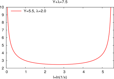
which we have displayed in Fig.2 (useful for correlations).
Refer to caption
Figure 2: Behavior of Q~​(ΞΌ,Ο…)~π‘„πœ‡πœ\widetilde{Q}(\mu,\upsilon) as a function of β„“=ln⁑(1/x)β„“1π‘₯\ell=\ln(1/x).

Inserting (31b) and (32) into (31a) gives the SD logarithmic derivatives of the single inclusive distribution

Οˆβ„“β€‹(ΞΌ,Ο…)subscriptπœ“β„“πœ‡πœ\displaystyle\psi_{\ell}(\mu,\upsilon)\!\! =\displaystyle\!\!=\!\! Ξ³0​eΞΌ+12​a​γ02​[eμ​Q~​(ΞΌ,Ο…)βˆ’tanhβ‘Ο…βˆ’tanh⁑υ​coth⁑μ​(1+eμ​Q~​(ΞΌ,Ο…))]subscript𝛾0superscriptπ‘’πœ‡12π‘Žsuperscriptsubscript𝛾02delimited-[]superscriptπ‘’πœ‡~π‘„πœ‡πœπœπœhyperbolic-cotangentπœ‡1superscriptπ‘’πœ‡~π‘„πœ‡πœ\displaystyle\!\!\gamma_{0}e^{\mu}\!+\!\frac{1}{2}a\gamma_{0}^{2}\Big{[}e^{\mu}\widetilde{Q}(\mu,\upsilon)\!-\!\tanh\upsilon\!-\!\tanh\upsilon\coth\mu\Big{(}1\!+\!e^{\mu}\widetilde{Q}(\mu,\upsilon)\Big{)}\Big{]} (34c)
βˆ’12​β​γ02​[1+tanh⁑υ​(1+K​(ΞΌ,Ο…))+C​(ΞΌ,Ο…)​(1+eμ​Q~​(ΞΌ,Ο…))]+π’ͺ​(Ξ³02),12𝛽superscriptsubscript𝛾02delimited-[]1𝜐1πΎπœ‡πœπΆπœ‡πœ1superscriptπ‘’πœ‡~π‘„πœ‡πœπ’ͺsuperscriptsubscript𝛾02\displaystyle\hskip 8.5359pt-\frac{1}{2}\beta\gamma_{0}^{2}\Big{[}1\!+\!\tanh\upsilon\Big{(}1\!+\!K(\mu,\upsilon)\Big{)}+C(\mu,\upsilon)\Big{(}1\!+\!e^{\mu}\widetilde{Q}(\mu,\upsilon)\Big{)}\Big{]}+{\cal O}(\gamma_{0}^{2}),
ψy​(ΞΌ,Ο…)subscriptπœ“π‘¦πœ‡πœ\displaystyle\psi_{y}(\mu,\upsilon)\!\! =\displaystyle\!\!=\!\! Ξ³0​eβˆ’ΞΌβˆ’12​a​γ02​[2+eβˆ’ΞΌβ€‹Q~​(ΞΌ,Ο…)+tanhβ‘Ο…βˆ’tanh⁑υ​coth⁑μ​(1+eβˆ’ΞΌβ€‹Q~​(ΞΌ,Ο…))]subscript𝛾0superscriptπ‘’πœ‡12π‘Žsuperscriptsubscript𝛾02delimited-[]2superscriptπ‘’πœ‡~π‘„πœ‡πœπœπœhyperbolic-cotangentπœ‡1superscriptπ‘’πœ‡~π‘„πœ‡πœ\displaystyle\!\!\gamma_{0}e^{-\mu}\!-\!\frac{1}{2}a\gamma_{0}^{2}\Big{[}2\!+\!e^{-\mu}\widetilde{Q}(\mu,\upsilon)\!+\!\tanh\upsilon\!-\!\tanh\upsilon\coth\mu\Big{(}1\!+\!e^{-\mu}\widetilde{Q}(\mu,\upsilon)\Big{)}\Big{]} (34f)
βˆ’12​β​γ02​[1+tanh⁑υ​(1+K​(ΞΌ,Ο…))βˆ’C​(ΞΌ,Ο…)​(1+eβˆ’ΞΌβ€‹Q~​(ΞΌ,Ο…))]+π’ͺ​(Ξ³02)12𝛽superscriptsubscript𝛾02delimited-[]1𝜐1πΎπœ‡πœπΆπœ‡πœ1superscriptπ‘’πœ‡~π‘„πœ‡πœπ’ͺsuperscriptsubscript𝛾02\displaystyle\hskip 17.07182pt-\frac{1}{2}\beta\gamma_{0}^{2}\Big{[}1\!+\!\tanh\upsilon\Big{(}1\!+\!K(\mu,\upsilon)\Big{)}-C(\mu,\upsilon)\Big{(}1\!+\!e^{-\mu}\widetilde{Q}(\mu,\upsilon)\Big{)}\Big{]}+{\cal O}(\gamma_{0}^{2})

where we have introduced (L𝐿L and K𝐾K have been written in (85) and (86))

C​(ΞΌ,Ο…)=L​(ΞΌ,Ο…)+tanh⁑υ​coth⁑μ​(1+K​(ΞΌ,Ο…)).πΆπœ‡πœπΏπœ‡πœπœhyperbolic-cotangentπœ‡1πΎπœ‡πœC(\mu,\upsilon)=L(\mu,\upsilon)+\tanh\upsilon\coth\mu\Big{(}1+K(\mu,\upsilon)\Big{)}. (35)

C𝐢C does not diverge when ΞΌβˆΌΟ…β†’0similar-toπœ‡πœβ†’0\mu\sim\upsilon\to 0. One has indeed

limΞΌ,Ο…β†’0[L​(ΞΌ,Ο…)+tanh⁑υ​coth⁑μ​K​(ΞΌ,Ο…)]=limΞΌ,Ο…β†’02βˆ’3​υ2ΞΌ2βˆ’Ο…3ΞΌ34​(1βˆ’Ο…3ΞΌ3)​μ=0subscriptβ†’πœ‡πœ0delimited-[]πΏπœ‡πœπœhyperbolic-cotangentπœ‡πΎπœ‡πœsubscriptβ†’πœ‡πœ023superscript𝜐2superscriptπœ‡2superscript𝜐3superscriptπœ‡341superscript𝜐3superscriptπœ‡3πœ‡0\lim_{\mu,\upsilon\rightarrow 0}\left[L(\mu,\upsilon)+\tanh\upsilon\coth\mu K(\mu,\upsilon)\right]=\lim_{\mu,\upsilon\rightarrow 0}\frac{2-3\frac{\upsilon^{2}}{\mu^{2}}-\frac{\upsilon^{3}}{\mu^{3}}}{4\left(1-\frac{\upsilon^{3}}{\mu^{3}}\right)}\mu=0

as well as

limΞΌ,Ο…β†’0tanh⁑υ​coth⁑μ​(1+e±μ​Q~​(ΞΌ,Ο…))=limΞΌ,Ο…β†’0=3​υμ1βˆ’Ο…3ΞΌ3=3​λY+Ξ»1βˆ’(Ξ»Y+Ξ»)3/2.subscriptβ†’πœ‡πœ0𝜐hyperbolic-cotangentπœ‡1superscript𝑒plus-or-minusπœ‡~π‘„πœ‡πœsubscriptβ†’πœ‡πœ03πœπœ‡1superscript𝜐3superscriptπœ‡33πœ†π‘Œπœ†1superscriptπœ†π‘Œπœ†32\lim_{\mu,\upsilon\rightarrow 0}\tanh\upsilon\coth\mu\left(1+e^{\pm\mu}\widetilde{Q}(\mu,\upsilon)\right)=\lim_{\mu,\upsilon\rightarrow 0}=\frac{3\frac{\upsilon}{\mu}}{1-\frac{\upsilon^{3}}{\mu^{3}}}=\frac{3\sqrt{\frac{\lambda}{Y+\lambda}}}{1-\left(\frac{\lambda}{Y+\lambda}\right)^{3/2}}.

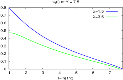
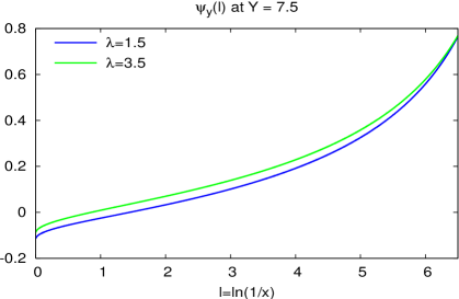
In (34c) and (34f) it is easy to keep trace of leading and sub-leading contributions. The first π’ͺ​(Ξ³0)π’ͺsubscript𝛾0{\cal O}(\gamma_{0}) term is DLA [7] while the second (∝aβ†’proportional-toabsentπ‘Žβ†’absent\propto a\to β€œhard corrections”) and third (βˆΞ²β†’proportional-toabsent𝛽→absent\propto\beta\to β€œrunning coupling effects”) terms are MLLA corrections (π’ͺ​(Ξ³02)π’ͺsuperscriptsubscript𝛾02{\cal O}(\gamma_{0}^{2})), of relative order π’ͺ​(Ξ³0)π’ͺsubscript𝛾0{\cal O}(\gamma_{0}) with respect to the leading one. In Fig.3 we plot (34c) (left) and (34f) (right) for two different values of Ξ»πœ†\lambda; one observes that Οˆβ„“subscriptπœ“β„“\psi_{\ell} (ψysubscriptπœ“π‘¦\psi_{y}) decreases (increases) when Ξ»πœ†\lambda increases.

Refer to caption
Refer to caption
Figure 3: SD logarithmic derivatives Οˆβ„“subscriptπœ“β„“\psi_{\ell} and ψysubscriptπœ“π‘¦\psi_{y} of the inclusive spectrum at Y=7.5π‘Œ7.5Y=7.5, for Ξ»=1.5πœ†1.5\lambda=1.5 and Ξ»=3.5πœ†3.5\lambda=3.5.

For further use in correlations, the logarithmic derivatives have the important property that they do not depend on the normalization but only on the shape of the single inclusive distribution.

2.4.1 β€œLimiting spectrum”: π€β†’πŸŽβ€‹(π‘ΈπŸŽ=πš²π‘Έβ€‹π‘ͺ​𝑫)bold-→𝝀0subscript𝑸0subscriptπš²π‘Έπ‘ͺ𝑫\boldsymbol{\lambda\to 0\ (Q_{0}=\Lambda_{QCD})}

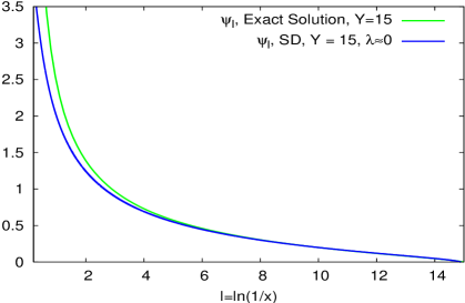
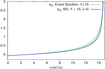
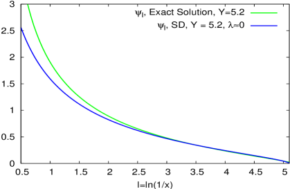
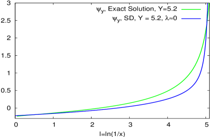
Since the logarithmic derivatives are β€œinfrared stable” (see above), we can take the limit Ξ»β†’0β†’πœ†0\lambda\to 0 in (34c)(34f) 444For this purpose, (18a) has been numerically inverted., and compare their shapes with the ones obtained in [5]; this is done in Figs.Β 4 and 5, at LEP-I energy (Eβ€‹Ξ˜0=91.2​GeV𝐸subscriptΘ091.2GeVE\Theta_{0}=91.2\,\text{GeV}, Y=5.2π‘Œ5.2Y=5.2) and at the unrealistic value Y=15π‘Œ15Y=15.

The agreement between the SD and the exact logarithmic derivatives is seen to be quite good. The small deviations (≀20%absentpercent20\leq 20\%) that can be observed at large β„“β„“\ell (the domain we deal with) arise from NMLLA corrections that one does not control in the exact solution. The agreement gets better and better as the energy increases.
Refer to caption
Refer to caption
Figure 4: SD logarithmic derivatives Οˆβ„“subscriptπœ“β„“\psi_{\ell} (left) and ψysubscriptπœ“π‘¦\psi_{y} (right) compared with the ones of [1] at Y=5.2π‘Œ5.2Y=5.2.
Refer to caption
Refer to caption
Figure 5: SD logarithmic derivatives Οˆβ„“subscriptπœ“β„“\psi_{\ell} (left) and ψysubscriptπœ“π‘¦\psi_{y} (right) compared with the ones of [1] at Y=15π‘Œ15Y=15.

It is checked in appendix (A.4) that (19) satisfies the evolution equation (2); the SD logarithmic derivatives (34c) and (34f) can therefore be used in the approximate calculation of 2-particle correlations at Ξ»β‰ 0πœ†0\lambda\neq 0. This is what is done in the next section.

3 2-PARTICLE CORRELATIONS INSIDE ONE JET AT π€β‰ πŸŽβ€‹(π‘ΈπŸŽβ‰ πš²π‘Έβ€‹π‘ͺ​𝑫)𝝀0subscript𝑸0subscriptπš²π‘Έπ‘ͺ𝑫\boldsymbol{\lambda\!\not=\!0\ (Q_{0}\!\neq\!\Lambda_{QCD})}

We study the correlation between 2-particles inside one jet of half opening angle ΘΘ\Theta within the MLLA accuracy. They have fixed energies x1=Ο‰1/Esubscriptπ‘₯1subscriptπœ”1𝐸x_{1}=\omega_{1}/E, x2=Ο‰2/Esubscriptπ‘₯2subscriptπœ”2𝐸x_{2}=\omega_{2}/E (Ο‰1>Ο‰2subscriptπœ”1subscriptπœ”2\omega_{1}>\omega_{2}) and are emitted at arbitrary angles Θ1subscriptΘ1\Theta_{1}, Θ2subscriptΘ2\Theta_{2}. The constrain Θ1β‰₯Θ2subscriptΘ1subscriptΘ2\Theta_{1}\geq\Theta_{2} follows from the angular ordering in the cascading process. One has Θβ‰₯Θ1ΘsubscriptΘ1\Theta\geq\Theta_{1} (see Fig.Β 1 of [1]).

3.1 Variables and kinematics

The variables and kinematics of the cascading process are defined like in section 3.2 of [1].

3.2 MLLA evolution equations for correlations

The system of integral evolution equations for the quark and gluon jets two-particle correlation reads (see eqs.Β (65) and (66) of [1])

Q(2)​(β„“1,y2,Ξ·)βˆ’Q1​(β„“1,y1)​Q2​(β„“2,y2)superscript𝑄2subscriptβ„“1subscript𝑦2πœ‚subscript𝑄1subscriptβ„“1subscript𝑦1subscript𝑄2subscriptβ„“2subscript𝑦2\displaystyle\hskip-25.6073ptQ^{(2)}(\ell_{1},y_{2},\eta)\!-\!Q_{1}(\ell_{1},y_{1})Q_{2}(\ell_{2},y_{2})\!\!\! =\displaystyle\!\!=\!\! CFNcβ€‹βˆ«0β„“1π‘‘β„“β€‹βˆ«0y2𝑑y​γ02​(β„“+y)​[1βˆ’34​δ​(β„“βˆ’β„“1)]​G(2)​(β„“,y,Ξ·),subscript𝐢𝐹subscript𝑁𝑐superscriptsubscript0subscriptβ„“1differential-dβ„“superscriptsubscript0subscript𝑦2differential-d𝑦superscriptsubscript𝛾02ℓ𝑦delimited-[]134𝛿ℓsubscriptβ„“1superscript𝐺2β„“π‘¦πœ‚\displaystyle\!\!\!\frac{C_{F}}{N_{c}}\!\!\int_{0}^{\ell_{1}}\!\!\!d\ell\!\int_{0}^{y_{2}}\!\!\!dy\,\gamma_{0}^{2}(\ell+y)\Big{[}\!1\!-\!\frac{3}{4}\delta(\ell-\ell_{1})\!\Big{]}G^{(2)}(\ell,y,\eta), (36)
G(2)​(β„“1,y2,Ξ·)βˆ’G1​(β„“1,y1)​G2​(β„“2,y2)superscript𝐺2subscriptβ„“1subscript𝑦2πœ‚subscript𝐺1subscriptβ„“1subscript𝑦1subscript𝐺2subscriptβ„“2subscript𝑦2\displaystyle\hskip-25.6073ptG^{(2)}(\ell_{1},y_{2},\eta)-G_{1}(\ell_{1},y_{1})G_{2}(\ell_{2},y_{2})\!\!\! =\displaystyle\!\!\!=\!\!\! ∫0β„“1π‘‘β„“β€‹βˆ«0y2𝑑y​γ02​(β„“+y)​[1βˆ’a​δ​(β„“βˆ’β„“1)]​G(2)​(β„“,y,Ξ·)superscriptsubscript0subscriptβ„“1differential-dβ„“superscriptsubscript0subscript𝑦2differential-d𝑦superscriptsubscript𝛾02ℓ𝑦delimited-[]1π‘Žπ›Ώβ„“subscriptβ„“1superscript𝐺2β„“π‘¦πœ‚\displaystyle\!\!\!\!\int_{0}^{\ell_{1}}\!\!d\ell\!\int_{0}^{y_{2}}\!\!dy\,\gamma_{0}^{2}(\ell+y)\Big{[}\!1-a\delta(\ell-\ell_{1})\!\Big{]}G^{(2)}(\ell,y,\eta) (37)
+\displaystyle\!\!\!+\!\!\! (aβˆ’b)β€‹βˆ«0y2𝑑y​γ02​(β„“1+y)​G​(β„“1,y+Ξ·)​G​(β„“1+Ξ·,y).π‘Žπ‘superscriptsubscript0subscript𝑦2differential-d𝑦superscriptsubscript𝛾02subscriptβ„“1𝑦𝐺subscriptβ„“1π‘¦πœ‚πΊsubscriptβ„“1πœ‚π‘¦\displaystyle\!\!\!(a-b)\int_{0}^{y_{2}}dy\>\gamma_{0}^{2}(\ell_{1}+y)G(\ell_{1},y+\eta)G(\ell_{1}+\eta,y).

a is defined in (3) while

b=14​Nc​[113​Ncβˆ’43​nf​TR​(1βˆ’2​CFNc)2]=nf=30.915.𝑏14subscript𝑁𝑐delimited-[]113subscript𝑁𝑐43subscript𝑛𝑓subscript𝑇𝑅superscript12subscript𝐢𝐹subscript𝑁𝑐2superscriptsubscript𝑛𝑓30.915b=\frac{1}{4N_{c}}\bigg{[}\frac{11}{3}N_{c}-\frac{4}{3}n_{f}T_{R}\bigg{(}1-2\frac{C_{F}}{N_{c}}\bigg{)}^{2}\bigg{]}\stackrel{{\scriptstyle n_{f}=3}}{{=}}0.915. (38)

3.3 MLLA solution at π€β‰ πŸŽπ€0\boldsymbol{\lambda\neq 0}

The quark and gluon jet correlators π’žqsubscriptπ’žπ‘ž{\cal C}_{q} and π’žgsubscriptπ’žπ‘”{\cal C}_{g} have been exactly determined for any Ξ»πœ†\lambda in [1] by respectively setting Q(2)=π’žq​Q1​Q2superscript𝑄2subscriptπ’žπ‘žsubscript𝑄1subscript𝑄2Q^{(2)}={\cal C}_{q}Q_{1}Q_{2} and G(2)=π’žg​G1​G2superscript𝐺2subscriptπ’žπ‘”subscript𝐺1subscript𝐺2G^{(2)}={\cal C}_{g}G_{1}G_{2} into (36) and (37). In the present work we limit ourselves to the exact MLLA solution which consists in neglecting all π’ͺ​(Ξ³02)π’ͺsuperscriptsubscript𝛾02{\cal O}(\gamma_{0}^{2}) corrections in equations (64) and (84) of [1].

3.3.1 Gluon jet

At MLLA, the logarithmic derivatives of Οˆπœ“\psi (24) can be truncated to the saddle point derivatives Ο†β„“,Ο†ysubscriptπœ‘β„“subscriptπœ‘π‘¦\varphi_{\ell},\,\varphi_{y} of (17). The MLLA solution of (37) then reads (see (77) in [1])

π’žgβˆ’1β‰ˆM​L​L​A1βˆ’b​(Ο†1,β„“+Ο†2,β„“)βˆ’Ξ΄11+Δ¯+Ξ”β€²+Ξ΄1superscript𝑀𝐿𝐿𝐴subscriptπ’žπ‘”11𝑏subscriptπœ‘1β„“subscriptπœ‘2β„“subscript𝛿11Β―Ξ”superscriptΞ”β€²subscript𝛿1{\cal C}_{g}-1\stackrel{{\scriptstyle MLLA}}{{\approx}}\frac{1-b\left(\varphi_{1,\ell}+\varphi_{2,\ell}\right)-\delta_{1}}{1+\bar{\Delta}+\Delta^{\prime}+\delta_{1}} (39)

where we introduce

Δ¯=Ξ³0βˆ’2​(Ο†1,ℓ​φ2,y+Ο†1,y​φ2,β„“),Β―Ξ”superscriptsubscript𝛾02subscriptπœ‘1β„“subscriptπœ‘2𝑦subscriptπœ‘1𝑦subscriptπœ‘2β„“\displaystyle\bar{\Delta}=\gamma_{0}^{-2}\Big{(}\varphi_{1,\ell}\varphi_{2,y}+\varphi_{1,y}\varphi_{2,\ell}\Big{)}, (40)
Ξ”β€²=Ξ³0βˆ’2​(Ο†1,β„“β€‹Ξ΄β€‹Οˆ2,y+Ξ΄β€‹Οˆ1,y​φ2,β„“+Ξ΄β€‹Οˆ1,ℓ​φ2,y+Ο†1,yβ€‹Ξ΄β€‹Οˆ2,β„“);superscriptΞ”β€²superscriptsubscript𝛾02subscriptπœ‘1ℓ𝛿subscriptπœ“2𝑦𝛿subscriptπœ“1𝑦subscriptπœ‘2ℓ𝛿subscriptπœ“1β„“subscriptπœ‘2𝑦subscriptπœ‘1𝑦𝛿subscriptπœ“2β„“\displaystyle\Delta^{\prime}=\gamma_{0}^{-2}\Big{(}\varphi_{1,\ell}\delta\psi_{2,y}+\delta\psi_{1,y}\varphi_{2,\ell}+\delta\psi_{1,\ell}\varphi_{2,y}+\varphi_{1,y}\delta\psi_{2,\ell}\Big{)}; (41)
Ο‡=ln⁑(1+11+Δ¯),Ο‡β„“=1Ο‡β€‹βˆ‚Ο‡βˆ‚β„“,Ο‡y=1Ο‡β€‹βˆ‚Ο‡βˆ‚y;formulae-sequenceπœ’111Β―Ξ”formulae-sequencesubscriptπœ’β„“1πœ’πœ’β„“subscriptπœ’π‘¦1πœ’πœ’π‘¦\displaystyle\chi=\ln\left(1+\frac{1}{1+\bar{\Delta}}\right),\quad\chi_{\ell}=\frac{1}{\chi}\frac{\partial\chi}{\partial\ell},\quad\chi_{y}=\frac{1}{\chi}\frac{\partial\chi}{\partial y}; (42)
Ξ΄1=Ξ³0βˆ’2​[χℓ​(Ο†1,y+Ο†2,y)+Ο‡y​(Ο†1,β„“+Ο†2,β„“)].subscript𝛿1superscriptsubscript𝛾02delimited-[]subscriptπœ’β„“subscriptπœ‘1𝑦subscriptπœ‘2𝑦subscriptπœ’π‘¦subscriptπœ‘1β„“subscriptπœ‘2β„“\displaystyle\delta_{1}=\gamma_{0}^{-2}\Big{[}\chi_{\ell}(\varphi_{1,y}+\varphi_{2,y})+\chi_{y}(\varphi_{1,\ell}+\varphi_{2,\ell})\Big{]}. (43)

(40) is obtained by using (26):

Δ¯​(ΞΌ1,ΞΌ2)=2​cosh⁑(ΞΌ1βˆ’ΞΌ2)=π’ͺ​(1),Β―Ξ”subscriptπœ‡1subscriptπœ‡22subscriptπœ‡1subscriptπœ‡2π’ͺ1\bar{\Delta}(\mu_{1},\mu_{2})=2\cosh(\mu_{1}-\mu_{2})={\cal O}(1), (44)

which is the DLA contribution [7], while (41) (see appendix B) is obtained by using (26), (31a) and (31b)

Δ′​(ΞΌ1,ΞΌ2)=eβˆ’ΞΌ1β€‹Ξ΄β€‹Οˆ2,β„“+eβˆ’ΞΌ2β€‹Ξ΄β€‹Οˆ1,β„“+eΞΌ1β€‹Ξ΄β€‹Οˆ2,y+eΞΌ2β€‹Ξ΄β€‹Οˆ1,yΞ³0=π’ͺ​(Ξ³0);superscriptΞ”β€²subscriptπœ‡1subscriptπœ‡2superscript𝑒subscriptπœ‡1𝛿subscriptπœ“2β„“superscript𝑒subscriptπœ‡2𝛿subscriptπœ“1β„“superscript𝑒subscriptπœ‡1𝛿subscriptπœ“2𝑦superscript𝑒subscriptπœ‡2𝛿subscriptπœ“1𝑦subscript𝛾0π’ͺsubscript𝛾0\Delta^{\prime}(\mu_{1},\mu_{2})=\frac{e^{-\mu_{1}}\delta\psi_{2,\ell}+e^{-\mu_{2}}\delta\psi_{1,\ell}+e^{\mu_{1}}\delta\psi_{2,y}+e^{\mu_{2}}\delta\psi_{1,y}}{\gamma_{0}}={\cal O}(\gamma_{0}); (45)

it is a next-to-leading (MLLA) correction. To get (42), we first use (44), which gives

Ο‡β„“=βˆ’tanh⁑μ1βˆ’ΞΌ221+2​cosh⁑(ΞΌ1βˆ’ΞΌ2)​(βˆ‚ΞΌ1βˆ‚β„“βˆ’βˆ‚ΞΌ2βˆ‚β„“),Ο‡y=βˆ’tanh⁑μ1βˆ’ΞΌ221+2​cosh⁑(ΞΌ1βˆ’ΞΌ2)​(βˆ‚ΞΌ1βˆ‚yβˆ’βˆ‚ΞΌ2βˆ‚y),formulae-sequencesubscriptπœ’β„“subscriptπœ‡1subscriptπœ‡2212subscriptπœ‡1subscriptπœ‡2subscriptπœ‡1β„“subscriptπœ‡2β„“subscriptπœ’π‘¦subscriptπœ‡1subscriptπœ‡2212subscriptπœ‡1subscriptπœ‡2subscriptπœ‡1𝑦subscriptπœ‡2𝑦\displaystyle\chi_{\ell}=-\frac{\tanh{\frac{\mu_{1}-\mu_{2}}{2}}}{1+2\cosh(\mu_{1}\!-\!\mu_{2})}\left(\frac{\partial\mu_{1}}{\partial\ell}-\frac{\partial\mu_{2}}{\partial\ell}\right),\quad\chi_{y}=-\frac{\tanh{\frac{\mu_{1}-\mu_{2}}{2}}}{1+2\cosh(\mu_{1}\!-\!\mu_{2})}\left(\frac{\partial\mu_{1}}{\partial y}-\frac{\partial\mu_{2}}{\partial y}\right), (46)

and then (32) to get

Ο‡β„“=β​γ02​tanh⁑μ1βˆ’ΞΌ221+2​cosh⁑(ΞΌ1βˆ’ΞΌ2)​eΞΌ1​Q~1βˆ’eΞΌ2​Q~22,Ο‡y=βˆ’Ξ²β€‹Ξ³02​tanh⁑μ1βˆ’ΞΌ221+2​cosh⁑(ΞΌ1βˆ’ΞΌ2)​eβˆ’ΞΌ1​Q~1βˆ’eβˆ’ΞΌ2​Q~22formulae-sequencesubscriptπœ’β„“π›½superscriptsubscript𝛾02subscriptπœ‡1subscriptπœ‡2212subscriptπœ‡1subscriptπœ‡2superscript𝑒subscriptπœ‡1subscript~𝑄1superscript𝑒subscriptπœ‡2subscript~𝑄22subscriptπœ’π‘¦π›½superscriptsubscript𝛾02subscriptπœ‡1subscriptπœ‡2212subscriptπœ‡1subscriptπœ‡2superscript𝑒subscriptπœ‡1subscript~𝑄1superscript𝑒subscriptπœ‡2subscript~𝑄22\displaystyle\chi_{\ell}\!=\!\beta\gamma_{0}^{2}\,\frac{\tanh{\frac{\mu_{1}-\mu_{2}}{2}}}{1\!+\!2\cosh(\mu_{1}\!-\!\mu_{2})}\>\frac{e^{\mu_{1}}\widetilde{Q}_{1}-e^{\mu_{2}}\widetilde{Q}_{2}}{2},\quad\chi_{y}\!=\!-\beta\gamma_{0}^{2}\frac{\tanh{\frac{\mu_{1}-\mu_{2}}{2}}}{1\!+\!2\cosh(\mu_{1}\!-\!\mu_{2})}\>\frac{e^{-\mu_{1}}\widetilde{Q}_{1}-e^{-\mu_{2}}\widetilde{Q}_{2}}{2}

which are π’ͺ​(Ξ³02)π’ͺsuperscriptsubscript𝛾02{\cal O}(\gamma_{0}^{2}). They should be plugged into (43) together with (26), which gives

Ξ΄1=β​γ0​2​sinh2⁑(ΞΌ1βˆ’ΞΌ22)3+4​sinh2⁑(ΞΌ1βˆ’ΞΌ22)​(Q~​(ΞΌ1,Ο…1)+Q~​(ΞΌ2,Ο…2))=π’ͺ​(Ξ³0);subscript𝛿1𝛽subscript𝛾02superscript2subscriptπœ‡1subscriptπœ‡2234superscript2subscriptπœ‡1subscriptπœ‡22~𝑄subscriptπœ‡1subscript𝜐1~𝑄subscriptπœ‡2subscript𝜐2π’ͺsubscript𝛾0\delta_{1}=\beta\gamma_{0}\frac{2\sinh^{2}{\left(\frac{\mu_{1}-\mu_{2}}{2}\right)}}{3+4\sinh^{2}{\left(\frac{\mu_{1}-\mu_{2}}{2}\right)}}\Big{(}\widetilde{Q}(\mu_{1},\upsilon_{1})+\widetilde{Q}(\mu_{2},\upsilon_{2})\Big{)}={\cal O}(\gamma_{0}); (47)

it is also a MLLA term. For Q≫Q0β‰₯Ξ›Q​C​Dmuch-greater-than𝑄subscript𝑄0subscriptΛ𝑄𝐢𝐷Q\gg Q_{0}\geq\Lambda_{QCD} we finally get,

π’žg​(β„“1,β„“2,Y,Ξ»)β‰ˆM​L​L​A1+1βˆ’b​γ0​(eΞΌ1+eΞΌ2)βˆ’Ξ΄11+2​cosh⁑(ΞΌ1βˆ’ΞΌ2)+Δ′​(ΞΌ1,ΞΌ2)+Ξ΄1superscript𝑀𝐿𝐿𝐴subscriptπ’žπ‘”subscriptβ„“1subscriptβ„“2π‘Œπœ†11𝑏subscript𝛾0superscript𝑒subscriptπœ‡1superscript𝑒subscriptπœ‡2subscript𝛿112subscriptπœ‡1subscriptπœ‡2superscriptΞ”β€²subscriptπœ‡1subscriptπœ‡2subscript𝛿1{\cal C}_{g}(\ell_{1},\ell_{2},Y,\lambda)\stackrel{{\scriptstyle MLLA}}{{\approx}}1+\frac{1-b\gamma_{0}\left(e^{\mu_{1}}+e^{\mu_{2}}\right)-\delta_{1}}{1+2\cosh(\mu_{1}-\mu_{2})+\Delta^{\prime}(\mu_{1},\mu_{2})+\delta_{1}} (48)

where the expression for Ξ”β€²superscriptΞ”β€²\Delta^{\prime} (92) is written in appendix B. It is important to notice that Ξ΄1≃0similar-to-or-equalssubscript𝛿10\delta_{1}\simeq 0 near β„“1β‰ˆβ„“2subscriptβ„“1subscriptβ„“2\ell_{1}\approx\ell_{2} (ΞΌ1β‰ˆΞΌ2subscriptπœ‡1subscriptπœ‡2\mu_{1}\approx\mu_{2}) while it is positive and increases as Ξ·πœ‚\eta gets larger (see (33) and Fig.2); it makes the correlation function narrower in |β„“1βˆ’β„“2|subscriptβ„“1subscriptβ„“2|\ell_{1}-\ell_{2}|.

3.3.2 Quark jet

The MLLA solution of (36) reads (see (93) in [1])

π’žqβˆ’1π’žgβˆ’1β‰ˆM​L​L​ANcCF​[1+(bβˆ’a)​(Ο•1,β„“+Ο•2,β„“)​1+Δ¯2+Δ¯]superscript𝑀𝐿𝐿𝐴subscriptπ’žπ‘ž1subscriptπ’žπ‘”1subscript𝑁𝑐subscript𝐢𝐹delimited-[]1π‘π‘Žsubscriptitalic-Ο•1β„“subscriptitalic-Ο•2β„“1Β―Ξ”2Β―Ξ”\displaystyle\frac{{\cal C}_{q}-1}{{\cal C}_{g}-1}\stackrel{{\scriptstyle MLLA}}{{\approx}}\frac{N_{c}}{C_{F}}\bigg{[}1+(b-a)(\phi_{1,\ell}+\phi_{2,\ell})\frac{1+\bar{\Delta}}{2+\bar{\Delta}}\bigg{]} (49)

Inserting (40)-(43) into (49) we get

π’žq​(β„“1,β„“2,Y,Ξ»)β‰ˆM​L​L​A1+NcCF​(π’žg​(β„“1,β„“2,Y,Ξ»)βˆ’1)​[1+(bβˆ’a)​γ0​(eΞΌ1+eΞΌ2)​1+2​cosh⁑(ΞΌ1βˆ’ΞΌ2)2+2​cosh⁑(ΞΌ1βˆ’ΞΌ2)].superscript𝑀𝐿𝐿𝐴subscriptπ’žπ‘žsubscriptβ„“1subscriptβ„“2π‘Œπœ†1subscript𝑁𝑐subscript𝐢𝐹subscriptπ’žπ‘”subscriptβ„“1subscriptβ„“2π‘Œπœ†1delimited-[]1π‘π‘Žsubscript𝛾0superscript𝑒subscriptπœ‡1superscript𝑒subscriptπœ‡212subscriptπœ‡1subscriptπœ‡222subscriptπœ‡1subscriptπœ‡2{\cal C}_{q}(\ell_{1},\ell_{2},Y,\lambda)\stackrel{{\scriptstyle MLLA}}{{\approx}}1+\frac{N_{c}}{C_{F}}\Big{(}{\cal C}_{g}(\ell_{1},\ell_{2},Y,\lambda)-1\Big{)}\bigg{[}1+(b-a)\gamma_{0}(e^{\mu_{1}}+e^{\mu_{2}})\frac{1+2\cosh(\mu_{1}-\mu_{2})}{2+2\cosh(\mu_{1}-\mu_{2})}\bigg{]}.

which finally reduces (for Q≫Q0β‰₯Ξ›Q​C​Dmuch-greater-than𝑄subscript𝑄0subscriptΛ𝑄𝐢𝐷Q\gg Q_{0}\geq\Lambda_{QCD}) to

π’žq​(β„“1,β„“2,Y,Ξ»)β‰ˆM​L​L​A1+NcCF​[(π’žg​(β„“1,β„“2,Y,Ξ»)βˆ’1)+12​(bβˆ’a)​γ0​eΞΌ1+eΞΌ21+cosh⁑(ΞΌ1βˆ’ΞΌ2)].superscript𝑀𝐿𝐿𝐴subscriptπ’žπ‘žsubscriptβ„“1subscriptβ„“2π‘Œπœ†1subscript𝑁𝑐subscript𝐢𝐹delimited-[]subscriptπ’žπ‘”subscriptβ„“1subscriptβ„“2π‘Œπœ†112π‘π‘Žsubscript𝛾0superscript𝑒subscriptπœ‡1superscript𝑒subscriptπœ‡21subscriptπœ‡1subscriptπœ‡2{\cal C}_{q}(\ell_{1},\ell_{2},Y,\lambda)\stackrel{{\scriptstyle MLLA}}{{\approx}}1+\frac{N_{c}}{C_{F}}\bigg{[}\Big{(}{\cal C}_{g}(\ell_{1},\ell_{2},Y,\lambda)-1\Big{)}+\frac{1}{2}(b-a)\gamma_{0}\frac{e^{\mu_{1}}+e^{\mu_{2}}}{1+\cosh(\mu_{1}-\mu_{2})}\bigg{]}. (50)

3.4 Sensitivity of the quark and gluon jets correlators to the value of 𝝀𝝀\boldsymbol{\lambda}

Increasing Ξ»πœ†\lambda translates into taking the limits Ξ²,Ξ›Q​C​Dβ†’0→𝛽subscriptΛ𝑄𝐢𝐷0\beta,\,\Lambda_{QCD}\to 0 (Y=β„“+yβ‰ͺΞ»,Q≫Q0≫ΛQ​C​Dformulae-sequenceπ‘Œβ„“π‘¦much-less-thanπœ†much-greater-than𝑄subscript𝑄0much-greater-thansubscriptΛ𝑄𝐢𝐷Y=\ell+y\ll\lambda,\,Q\gg Q_{0}\gg\Lambda_{QCD}) in the definition of the anomalous dimension via the running coupling constant (Ξ³0=Ξ³0​(Ξ±s)subscript𝛾0subscript𝛾0subscript𝛼𝑠\gamma_{0}=\gamma_{0}(\alpha_{s}), see (44) in [1]). It allows to neglect β„“β„“\ell, y𝑦y with respect to Ξ»πœ†\lambda as follows

Ξ³02​(β„“+y)=1β​(β„“+y+Ξ»)β‰ˆβ„“+yβ‰ͺλγ02=1β​λ,superscriptsubscript𝛾02ℓ𝑦1π›½β„“π‘¦πœ†superscriptmuch-less-thanβ„“π‘¦πœ†superscriptsubscript𝛾021π›½πœ†\gamma_{0}^{2}(\ell+y)=\frac{1}{\beta(\ell+y+\lambda)}\stackrel{{\scriptstyle\ell+y\ll\lambda}}{{\approx}}\gamma_{0}^{2}=\frac{1}{\beta\lambda}, (51)

such that Ξ³0subscript𝛾0\gamma_{0} can be taken as a constant. Estimating (4) in the region λ≫1⇔sβ‰ͺ1⇔much-greater-thanπœ†1much-less-than𝑠1\lambda\gg 1\Leftrightarrow s\ll 1 needs evaluating the kernel

1Ξ½+s​(ω​(Ξ½+s)(Ο‰+s)​ν)1/β​(Ο‰βˆ’Ξ½)​(Ξ½Ξ½+s)a/Ξ²1πœˆπ‘ superscriptπœ”πœˆπ‘ πœ”π‘ πœˆ1π›½πœ”πœˆsuperscriptπœˆπœˆπ‘ π‘Žπ›½\displaystyle\frac{1}{\nu+s}\left(\frac{\omega\left(\nu+s\right)}{\left(\omega+s\right)\nu}\right)^{1/\beta\left(\omega-\nu\right)}\!\!\left(\frac{\nu}{\nu+s}\right)^{a/\beta}\!\! β‰ˆsβ‰ͺ1superscriptmuch-less-than𝑠1\displaystyle\!\!\stackrel{{\scriptstyle s\ll 1}}{{\approx}}\!\! 1ν​(1+Ο‰βˆ’Ξ½Ο‰β€‹Ξ½β€‹s)1/β​(Ο‰βˆ’Ξ½)​(1βˆ’sΞ½)a/Ξ²1𝜈superscript1πœ”πœˆπœ”πœˆπ‘ 1π›½πœ”πœˆsuperscript1π‘ πœˆπ‘Žπ›½\displaystyle\!\!\frac{1}{\nu}\left(1+\frac{\omega-\nu}{\omega\nu}s\right)^{1/\beta\left(\omega-\nu\right)}\left(1-\frac{s}{\nu}\right)^{a/\beta} (54)
β‰ˆ1ν​[1+1ν​(1Ο‰βˆ’a)​sΞ²+12!​1Ξ½2​(1Ο‰βˆ’a)2​s2Ξ²2+13!​1Ξ½3​(1Ο‰βˆ’a)3​s3Ξ²3+…].absent1𝜈delimited-[]11𝜈1πœ”π‘Žπ‘ π›½121superscript𝜈2superscript1πœ”π‘Ž2superscript𝑠2superscript𝛽2131superscript𝜈3superscript1πœ”π‘Ž3superscript𝑠3superscript𝛽3…\displaystyle\hskip-199.16928pt\approx\frac{1}{\nu}\left[1+\frac{1}{\nu}\left(\frac{1}{\omega}-a\right)\frac{s}{\beta}+\frac{1}{2!}\frac{1}{\nu^{2}}\left(\frac{1}{\omega}-a\right)^{2}\frac{s^{2}}{\beta^{2}}+\frac{1}{3!}\frac{1}{\nu^{3}}\left(\frac{1}{\omega}-a\right)^{3}\frac{s^{3}}{\beta^{3}}+\dots\right].

Integrating (54) over s𝑠s, using (51) and ∫0∞sn​eβˆ’Ξ»β€‹s=n!Ξ»nsuperscriptsubscript0superscript𝑠𝑛superscriptπ‘’πœ†π‘ π‘›superscriptπœ†π‘›\int_{0}^{\infty}s^{n}\,e^{-\lambda s}=\frac{n!}{\lambda^{n}}, we get

𝒒​(Ο‰,Ξ½)π’’πœ”πœˆ\displaystyle{\cal{G}}(\omega,\nu)\!\! β‰ˆ\displaystyle\!\!\approx\!\! 1ν​[1+1ν​(1Ο‰βˆ’a)​1β​λ+1Ξ½2​(1Ο‰βˆ’a)2​(1β​λ)2+1Ξ½3​(1Ο‰βˆ’a)3​(1β​λ)3+…]1𝜈delimited-[]11𝜈1πœ”π‘Ž1π›½πœ†1superscript𝜈2superscript1πœ”π‘Ž2superscript1π›½πœ†21superscript𝜈3superscript1πœ”π‘Ž3superscript1π›½πœ†3…\displaystyle\!\!\frac{1}{\nu}\left[1+\frac{1}{\nu}\left(\frac{1}{\omega}-a\right)\frac{1}{\beta\lambda}+\frac{1}{\nu^{2}}\left(\frac{1}{\omega}-a\right)^{2}\left(\frac{1}{\beta\lambda}\right)^{2}+\frac{1}{\nu^{3}}\left(\frac{1}{\omega}-a\right)^{3}\left(\frac{1}{\beta\lambda}\right)^{3}+\dots\right]
=\displaystyle\!\!=\!\! 1Ξ½βˆ’Ξ³02​(1/Ο‰βˆ’a),1𝜈superscriptsubscript𝛾021πœ”π‘Ž\displaystyle\!\!\frac{1}{\nu-\gamma_{0}^{2}\left(1/\omega-a\right)},

which, after inverting the Mellin’s representation (132) of [1], gives

G​(β„“,y)≃xβ‰ͺ1exp⁑(2​γ0​ℓ​yβˆ’a​γ02​y).superscriptsimilar-to-or-equalsmuch-less-thanπ‘₯1𝐺ℓ𝑦2subscript𝛾0β„“π‘¦π‘Žsuperscriptsubscript𝛾02𝑦G(\ell,y)\stackrel{{\scriptstyle x\ll 1}}{{\simeq}}\exp(2\gamma_{0}\sqrt{\ell\,y}-a\gamma_{0}^{2}y). (55)

Taking the same limit in (18a) and (18b) gives respectively

yβˆ’β„“y+β„“β‰ˆβ„“+yβ‰ͺΞ»tanh⁑μ⇒μ=12​ln⁑yβ„“,ΞΌβˆ’Ο…β‰ˆβ„“+yβ‰ͺΞ»12​yβˆ’β„“Ξ»β‡’ΞΌβˆΌΟ….formulae-sequencesuperscriptmuch-less-thanβ„“π‘¦πœ†π‘¦β„“π‘¦β„“πœ‡β‡’πœ‡12𝑦ℓsuperscriptmuch-less-thanβ„“π‘¦πœ†πœ‡πœ12π‘¦β„“πœ†β‡’πœ‡similar-to𝜐\frac{y-\ell}{y+\ell}\stackrel{{\scriptstyle\ell+y\ll\lambda}}{{\approx}}\tanh\mu\Rightarrow\mu=\frac{1}{2}\ln\frac{y}{\ell},\qquad\mu-\upsilon\stackrel{{\scriptstyle\ell+y\ll\lambda}}{{\approx}}\frac{1}{2}\frac{y-\ell}{\lambda}\Rightarrow\mu\sim\upsilon. (56)

Furthermore, we use (56) to show how (24) reduces to the exponent in (55) 555we set Ξ²=0𝛽0\beta=0 in (34c), (34f) and only consider terms ∝aproportional-toabsentπ‘Ž\propto a

Ο•italic-Ο•\displaystyle\phi\!\! =\displaystyle\!\!=\!\! 2Ξ²β€‹ΞΌβˆ’Ο…sinhβ‘ΞΌβˆ’sinhβ‘Ο…β‰ˆβ„“+yβ‰ͺΞ»2​γ0​ℓ​y,superscriptmuch-less-thanβ„“π‘¦πœ†2π›½πœ‡πœπœ‡πœ2subscript𝛾0ℓ𝑦\displaystyle\!\!\frac{2}{\sqrt{\beta}}\frac{\mu-\upsilon}{\sinh\mu-\sinh\upsilon}\stackrel{{\scriptstyle\ell+y\ll\lambda}}{{\approx}}2\gamma_{0}\sqrt{\ell\,y}, (57)
(Ξ½0Ξ½0+s0)a/Ξ²superscriptsubscript𝜈0subscript𝜈0subscript𝑠0π‘Žπ›½\displaystyle\left(\frac{\nu_{0}}{\nu_{0}+s_{0}}\right)^{a/\beta}\!\! =\displaystyle\!\!=\!\! βˆ’12​aβ​ln⁑(1+β„“+yΞ»)βˆ’aβ​(ΞΌβˆ’Ο…)β‰ˆβˆ’12​aβ​ℓ+yΞ»βˆ’aβ​(ΞΌβˆ’Ο…)12π‘Žπ›½1β„“π‘¦πœ†π‘Žπ›½πœ‡πœ12π‘Žπ›½β„“π‘¦πœ†π‘Žπ›½πœ‡πœ\displaystyle\!\!-\frac{1}{2}\frac{a}{\beta}\ln\left(1+\frac{\ell+y}{\lambda}\right)-\frac{a}{\beta}(\mu-\upsilon)\approx-\frac{1}{2}\frac{a}{\beta}\frac{\ell+y}{\lambda}-\frac{a}{\beta}(\mu-\upsilon) (60)
β‰ˆβ„“+yβ‰ͺΞ»superscriptmuch-less-thanβ„“π‘¦πœ†\displaystyle\!\!\stackrel{{\scriptstyle\ell+y\ll\lambda}}{{\approx}}\!\! βˆ’a​γ02​y.π‘Žsuperscriptsubscript𝛾02𝑦\displaystyle\!\!-a\gamma_{0}^{2}\,y. (62)

Thus, since ΞΌ=12​ln⁑yβ„“πœ‡12𝑦ℓ\mu=\frac{1}{2}\ln\frac{y}{\ell} (56), (34c) and (34f) simplify to

Οˆβ„“β‰ˆβ„“+yβ‰ͺλγ0​eΞΌ=Ξ³0​yβ„“,ψyβ‰ˆβ„“+yβ‰ͺλγ0​eβˆ’ΞΌβˆ’a​γ02=Ξ³0​ℓyβˆ’a​γ02.formulae-sequencesuperscriptmuch-less-thanβ„“π‘¦πœ†subscriptπœ“β„“subscript𝛾0superscriptπ‘’πœ‡subscript𝛾0𝑦ℓsuperscriptmuch-less-thanβ„“π‘¦πœ†subscriptπœ“π‘¦subscript𝛾0superscriptπ‘’πœ‡π‘Žsuperscriptsubscript𝛾02subscript𝛾0β„“π‘¦π‘Žsuperscriptsubscript𝛾02\psi_{\ell}\stackrel{{\scriptstyle\ell+y\ll\lambda}}{{\approx}}\gamma_{0}e^{\mu}=\gamma_{0}\sqrt{\frac{y}{\ell}},\qquad\psi_{y}\stackrel{{\scriptstyle\ell+y\ll\lambda}}{{\approx}}\gamma_{0}e^{-\mu}-a\gamma_{0}^{2}=\gamma_{0}\sqrt{\frac{\ell}{y}}-a\gamma_{0}^{2}. (63)

Therefore, taking the limit Ξ²,Ξ›Q​C​Dβ†’0→𝛽subscriptΛ𝑄𝐢𝐷0\beta,\,\Lambda_{QCD}\to 0 (Ξ»β†’βˆžβ†’πœ†\lambda\to\infty) leads to the simplified model described in section 4.2 of [1]. Setting, for the sake of simplicity, β„“1β‰ˆβ„“2subscriptβ„“1subscriptβ„“2\ell_{1}\approx\ell_{2} in (48)(49), where Ξ΄1subscript𝛿1\delta_{1} vanishes, we obtain, in the high energy limit

π’žg​(β„“,y)≃1+13​[1βˆ’2​(bβˆ’13​a)β€‹Οˆβ„“β€‹(β„“,y)],π’žq​(β„“,y)≃1+NcCF​[13βˆ’12​(53​a+b)β€‹Οˆβ„“β€‹(β„“,y)],formulae-sequencesimilar-to-or-equalssubscriptπ’žπ‘”β„“π‘¦113delimited-[]12𝑏13π‘Žsubscriptπœ“β„“β„“π‘¦similar-to-or-equalssubscriptπ’žπ‘žβ„“π‘¦1subscript𝑁𝑐subscript𝐢𝐹delimited-[]131253π‘Žπ‘subscriptπœ“β„“β„“π‘¦{\cal C}_{g}(\ell,y)\simeq 1\!+\!\frac{1}{3}\left[1\!-\!2\left(b\!-\!\frac{1}{3}a\right)\psi_{\ell}(\ell,y)\right],\quad{\cal C}_{q}(\ell,y)\simeq 1\!+\!\frac{N_{c}}{C_{F}}\left[\frac{1}{3}\!-\!\frac{1}{2}\left(\frac{5}{3}a\!+\!b\right)\psi_{\ell}(\ell,y)\right], (64)

where

bβˆ’13​a=118​(11βˆ’8​TRNc+28​TRNc​CFNcβˆ’24​TRNc​CF2Nc2)β‰ˆnf=30.6,𝑏13π‘Ž118118subscript𝑇𝑅subscript𝑁𝑐28subscript𝑇𝑅subscript𝑁𝑐subscript𝐢𝐹subscript𝑁𝑐24subscript𝑇𝑅subscript𝑁𝑐superscriptsubscript𝐢𝐹2superscriptsubscript𝑁𝑐2superscriptsubscript𝑛𝑓30.6\displaystyle b-\frac{1}{3}a=\frac{1}{18}\left(11-8\frac{T_{R}}{N_{c}}+28\frac{T_{R}}{N_{c}}\frac{C_{F}}{N_{c}}-24\frac{T_{R}}{N_{c}}\frac{C_{F}^{2}}{N_{c}^{2}}\right)\stackrel{{\scriptstyle n_{f}=3}}{{\approx}}0.6, (65)
(66)
(67)
53​a+b=29​(11+TRNc+TRNc​CFNcβˆ’6​TRNc​CF2Nc2)β‰ˆnf=32.5.53π‘Žπ‘2911subscript𝑇𝑅subscript𝑁𝑐subscript𝑇𝑅subscript𝑁𝑐subscript𝐢𝐹subscript𝑁𝑐6subscript𝑇𝑅subscript𝑁𝑐superscriptsubscript𝐢𝐹2superscriptsubscript𝑁𝑐2superscriptsubscript𝑛𝑓32.5\displaystyle\frac{5}{3}a+b=\frac{2}{9}\left(11+\frac{T_{R}}{N_{c}}+\frac{T_{R}}{N_{c}}\frac{C_{F}}{N_{c}}-6\frac{T_{R}}{N_{c}}\frac{C_{F}^{2}}{N_{c}^{2}}\right)\stackrel{{\scriptstyle n_{f}=3}}{{\approx}}2.5. (68)

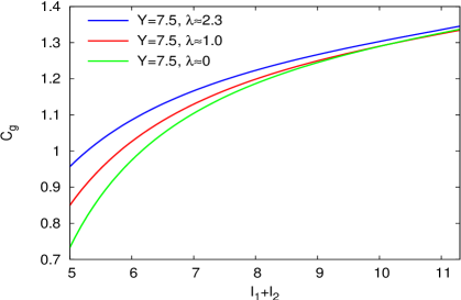
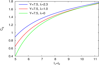
Thus, when Ξ»πœ†\lambda increases by decreasing Ξ›Q​C​DsubscriptΛ𝑄𝐢𝐷\Lambda_{QCD}, Οˆβ„“βˆΞ³0proportional-tosubscriptπœ“β„“subscript𝛾0\psi_{\ell}\!\propto\!\gamma_{0} decreases and the correlators (64) increase. For LHC, a typical value is Y=7.5π‘Œ7.5Y=7.5 and we compare in Fig.Β 6, at fixed Q0subscript𝑄0Q_{0}, the limiting case Ξ»β‰ˆ0πœ†0\lambda\approx 0 (Q0β‰ˆΞ›Q​C​Dβ‰ˆ253​MeVsubscript𝑄0subscriptΛ𝑄𝐢𝐷253MeVQ_{0}\approx\Lambda_{QCD}\approx 253\,\text{MeV}) with Ξ»β‰ˆ1.0πœ†1.0\lambda\approx 1.0 (Ξ›Q​C​D=100​MeVsubscriptΛ𝑄𝐢𝐷100MeV\Lambda_{QCD}=100\,\text{MeV}) and Ξ»β‰ˆ2.3πœ†2.3\lambda\approx 2.3 (Ξ›Q​C​D=25​MeVsubscriptΛ𝑄𝐢𝐷25MeV\Lambda_{QCD}=25\,\text{MeV}). As predicted by (64), the correlation increases when Ξ›Q​C​Dβ†’0β†’subscriptΛ𝑄𝐢𝐷0\Lambda_{QCD}\to 0 at fixed Q0subscript𝑄0Q_{0}.

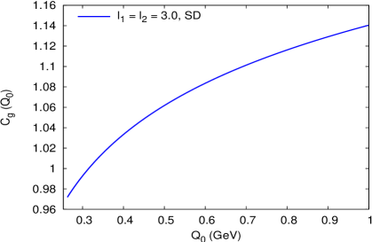
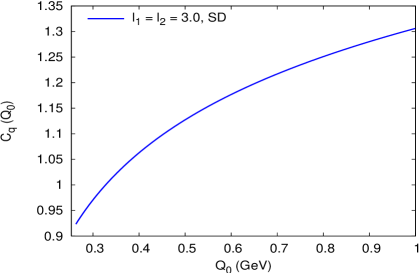
It is also sensitive to the value of Q0subscript𝑄0Q_{0}. As seen in (64), since y=ln⁑QQ0βˆ’β„“π‘¦π‘„subscript𝑄0β„“y=\ln\frac{Q}{Q_{0}}-\ell, if one increases Q0subscript𝑄0Q_{0} (since Ξ›Q​C​DsubscriptΛ𝑄𝐢𝐷\Lambda_{QCD} is fixed, Ξ³0subscript𝛾0\gamma_{0} does not change), thereby reducing the available phase space, the correlators increase. This dependence of the correlators at fixed Ξ›Q​C​DsubscriptΛ𝑄𝐢𝐷\Lambda_{QCD} is displayed in Fig.7 for 0.3​GeV≀Q0≀1.0​GeV0.3GeVsubscript𝑄01.0GeV0.3\,\text{GeV}\leq Q_{0}\leq 1.0\,\text{GeV} at β„“1=β„“2=3.0subscriptβ„“1subscriptβ„“23.0\ell_{1}=\ell_{2}=3.0 (soft parton).

Refer to caption
Refer to caption
Figure 6: Varying Ξ»πœ†\lambda at fixed Q0subscript𝑄0Q_{0}; Ξ›Q​C​DsubscriptΛ𝑄𝐢𝐷\Lambda_{QCD} dependence of π’žgsubscriptπ’žπ‘”{\cal C}_{g} (left) and π’žqsubscriptπ’žπ‘ž{\cal C}_{q} (right)
Refer to caption
Refer to caption
Figure 7: Varying Ξ»πœ†\lambda at fixed Ξ›Q​C​D=253​M​e​VsubscriptΛ𝑄𝐢𝐷253𝑀𝑒𝑉\Lambda_{QCD}=253\,MeV; Q0subscript𝑄0Q_{0}-dependence of π’žgsubscriptπ’žπ‘”{\cal C}_{g} (left) and π’žqsubscriptπ’žπ‘ž{\cal C}_{q} (right) at β„“1=β„“2=3.0subscriptβ„“1subscriptβ„“23.0\ell_{1}=\ell_{2}=3.0

In the simplified model which leads to (64), π’žgsubscriptπ’žπ‘”{\cal C}_{g} and π’žqsubscriptπ’žπ‘ž{\cal C}_{q} respectively go to the asymptotic values 4/3434/3 and 1+Nc/3​CF1subscript𝑁𝑐3subscript𝐢𝐹1+N_{c}/3C_{F}. This is however not the case in the general situation Ξ²β‰ 0𝛽0\beta\not=0, as can be easily checked by using (34c) and (34f); for example, near the maximum of the distribution (μ∼vβ†’0similar-toπœ‡π‘£β†’0\mu\sim v\to 0), a contribution ∝λ3/2/[(Y+Ξ»)3/2βˆ’Ξ»3/2]proportional-toabsentsuperscriptπœ†32delimited-[]superscriptπ‘Œπœ†32superscriptπœ†32\propto\lambda^{3/2}/[(Y+\lambda)^{3/2}-\lambda^{3/2}] occurs in the term proportional to β𝛽\beta in (64) that yields negative values of Οˆβ„“subscriptπœ“β„“\psi_{\ell} when Ξ»πœ†\lambda increases.

3.5 Extension of the Fong and Webber expansion; its limit 𝝀=πŸŽπ€0\boldsymbol{\lambda=0}

In the Fong-Webber regime, the energies of the two registered particles stay very close to the peak of the inclusive hump-backed distribution that is, |β„“iβˆ’β„“m​a​x|β‰ͺΟƒβˆ[(Y+Ξ»)3/2βˆ’Ξ»3/2]1/2much-less-thansubscriptℓ𝑖subscriptβ„“π‘šπ‘Žπ‘₯𝜎proportional-tosuperscriptdelimited-[]superscriptπ‘Œπœ†32superscriptπœ†3212|\ell_{i}-\ell_{max}|\ll\sigma\propto[(Y+\lambda)^{3/2}-\lambda^{3/2}]^{1/2} (see (23)).

Near the maximum of the single inclusive distribution β„“1βˆΌβ„“2≃Y/2similar-tosubscriptβ„“1subscriptβ„“2similar-to-or-equalsπ‘Œ2\ell_{1}\sim\ell_{2}\simeq Y/2 (ΞΌ,Ο…β†’0β†’πœ‡πœ0\mu,\upsilon\to 0, see appendix A.2)

limΞΌ,Ο…β†’0C=(Ξ»Y+Ξ»)1/2,limΞΌ,Ο…β†’0Ki=32​υi2ΞΌi3βˆ’Ο…i3,limΞΌ,Ο…β†’0Q~=23+13​(Ξ»Y+Ξ»)3/2,formulae-sequencesubscriptβ†’πœ‡πœ0𝐢superscriptπœ†π‘Œπœ†12formulae-sequencesubscriptβ†’πœ‡πœ0subscript𝐾𝑖32subscriptsuperscript𝜐2𝑖subscriptsuperscriptπœ‡3𝑖subscriptsuperscript𝜐3𝑖subscriptβ†’πœ‡πœ0~𝑄2313superscriptπœ†π‘Œπœ†32\lim_{\mu,\upsilon\rightarrow 0}C=\left(\frac{\lambda}{Y+\lambda}\right)^{1/2},\quad\lim_{\mu,\upsilon\rightarrow 0}K_{i}=\frac{3}{2}\frac{\upsilon^{2}_{i}}{\mu^{3}_{i}-\upsilon^{3}_{i}},\quad\lim_{\mu,\upsilon\rightarrow 0}\widetilde{Q}=\frac{2}{3}+\frac{1}{3}\left(\frac{\lambda}{Y+\lambda}\right)^{3/2},

where C𝐢C, Kisubscript𝐾𝑖K_{i} and Q~~𝑄\tilde{Q} are defined in (35), (86) and (33). Keeping only the terms linear in ΞΌπœ‡\mu and the term quadratic in the difference (ΞΌ1βˆ’ΞΌ2)subscriptπœ‡1subscriptπœ‡2(\mu_{1}-\mu_{2}), one has

Δ¯+Δ′≃ℓ1βˆΌβ„“2≃Y/22+(ΞΌ1βˆ’ΞΌ2)2βˆ’a​γ0​(2+ΞΌ1+ΞΌ2)βˆ’Ξ²β€‹Ξ³0​[2+3​λ3/2(Y+Ξ»)3/2βˆ’Ξ»3/2]superscriptsimilar-to-or-equalssimilar-tosubscriptβ„“1subscriptβ„“2similar-to-or-equalsπ‘Œ2Β―Ξ”superscriptΞ”β€²2superscriptsubscriptπœ‡1subscriptπœ‡22π‘Žsubscript𝛾02subscriptπœ‡1subscriptπœ‡2𝛽subscript𝛾0delimited-[]23superscriptπœ†32superscriptπ‘Œπœ†32superscriptπœ†32\displaystyle\bar{\Delta}+\Delta^{\prime}\stackrel{{\scriptstyle\ell_{1}\sim\ell_{2}\simeq Y/2}}{{\simeq}}2+(\mu_{1}-\mu_{2})^{2}-a\gamma_{0}\left(2+\mu_{1}+\mu_{2}\right)-\beta\gamma_{0}\left[2+3\frac{\lambda^{3/2}}{(Y+\lambda)^{3/2}-\lambda^{3/2}}\right] (69)

and

Ξ΄1≃ℓ1βˆΌβ„“2≃Y/219​β​γ0​(ΞΌ1βˆ’ΞΌ2)2​[2+(Ξ»Y+Ξ»)3/2];superscriptsimilar-to-or-equalssimilar-tosubscriptβ„“1subscriptβ„“2similar-to-or-equalsπ‘Œ2subscript𝛿119𝛽subscript𝛾0superscriptsubscriptπœ‡1subscriptπœ‡22delimited-[]2superscriptπœ†π‘Œπœ†32\delta_{1}\stackrel{{\scriptstyle\ell_{1}\sim\ell_{2}\simeq Y/2}}{{\simeq}}\frac{1}{9}\beta\gamma_{0}(\mu_{1}-\mu_{2})^{2}\left[2+\left(\frac{\lambda}{Y+\lambda}\right)^{3/2}\right]; (70)

Ξ΄1subscript𝛿1\delta_{1} can be neglected, since Ξ³0​(ΞΌ1βˆ’ΞΌ2)2β‰ͺ(ΞΌ1βˆ’ΞΌ2)2β‰ͺ1much-less-thansubscript𝛾0superscriptsubscriptπœ‡1subscriptπœ‡22superscriptsubscriptπœ‡1subscriptπœ‡22much-less-than1\gamma_{0}(\mu_{1}-\mu_{2})^{2}\ll(\mu_{1}-\mu_{2})^{2}\ll 1. Then, in the same limit, (48), (50) become

π’žg0​(β„“1,β„“2,Y,Ξ»)≃ℓ1βˆΌβ„“2≃Y/21+1βˆ’b​γ0​(2+ΞΌ1+ΞΌ2)3+(ΞΌ1βˆ’ΞΌ2)2βˆ’a​γ0​(2+ΞΌ1+ΞΌ2)βˆ’Ξ²β€‹Ξ³0​[2+3​λ3/2(Y+Ξ»)3/2βˆ’Ξ»3/2],superscriptsimilar-to-or-equalssimilar-tosubscriptβ„“1subscriptβ„“2similar-to-or-equalsπ‘Œ2superscriptsubscriptπ’žπ‘”0subscriptβ„“1subscriptβ„“2π‘Œπœ†11𝑏subscript𝛾02subscriptπœ‡1subscriptπœ‡23superscriptsubscriptπœ‡1subscriptπœ‡22π‘Žsubscript𝛾02subscriptπœ‡1subscriptπœ‡2𝛽subscript𝛾0delimited-[]23superscriptπœ†32superscriptπ‘Œπœ†32superscriptπœ†32{\cal C}_{g}^{0}(\ell_{1},\ell_{2},Y,\lambda)\!\stackrel{{\scriptstyle\ell_{1}\sim\ell_{2}\simeq Y/2}}{{\simeq}}\!1\!+\!\frac{1-b\gamma_{0}(2+\mu_{1}+\mu_{2})}{3+(\mu_{1}-\mu_{2})^{2}-a\gamma_{0}\left(2+\mu_{1}+\mu_{2}\right)-\beta\gamma_{0}\left[2+3\displaystyle\frac{\lambda^{3/2}}{(Y+\lambda)^{3/2}-\lambda^{3/2}}\right]}, (71)
π’žq0​(β„“1,β„“2,Y,Ξ»)≃ℓ1βˆΌβ„“2≃Y/21+NcCF​[(π’žg0​(β„“1,β„“2,Y,Ξ»)βˆ’1)+14​(bβˆ’a)​γ0​(2+ΞΌ1+ΞΌ2)].superscriptsimilar-to-or-equalssimilar-tosubscriptβ„“1subscriptβ„“2similar-to-or-equalsπ‘Œ2superscriptsubscriptπ’žπ‘ž0subscriptβ„“1subscriptβ„“2π‘Œπœ†1subscript𝑁𝑐subscript𝐢𝐹delimited-[]superscriptsubscriptπ’žπ‘”0subscriptβ„“1subscriptβ„“2π‘Œπœ†114π‘π‘Žsubscript𝛾02subscriptπœ‡1subscriptπœ‡2{\cal C}_{q}^{0}(\ell_{1},\ell_{2},Y,\lambda)\stackrel{{\scriptstyle\ell_{1}\sim\ell_{2}\simeq Y/2}}{{\simeq}}1+\frac{N_{c}}{C_{F}}\bigg{[}\Big{(}{\cal C}_{g}^{0}(\ell_{1},\ell_{2},Y,\lambda)-1\Big{)}+\frac{1}{4}(b-a)\gamma_{0}\left(2+\mu_{1}+\mu_{2}\right)\bigg{]}. (72)

Using (82) one has

(ΞΌ1βˆ’ΞΌ2)2≃9​Y+Ξ»[(Y+Ξ»)3/2βˆ’Ξ»3/2]2​(β„“1βˆ’β„“2)2,ΞΌ1+ΞΌ2≃3​(Y+Ξ»)1/2(Y+Ξ»)3/2βˆ’Ξ»3/2​[Yβˆ’(β„“1+β„“2)]formulae-sequencesimilar-to-or-equalssuperscriptsubscriptπœ‡1subscriptπœ‡229π‘Œπœ†superscriptdelimited-[]superscriptπ‘Œπœ†32superscriptπœ†322superscriptsubscriptβ„“1subscriptβ„“22similar-to-or-equalssubscriptπœ‡1subscriptπœ‡23superscriptπ‘Œπœ†12superscriptπ‘Œπœ†32superscriptπœ†32delimited-[]π‘Œsubscriptβ„“1subscriptβ„“2(\mu_{1}\!-\!\mu_{2})^{2}\simeq 9\frac{Y+\lambda}{\left[(Y+\lambda)^{3/2}-\lambda^{3/2}\right]^{2}}(\ell_{1}-\ell_{2})^{2},\quad\mu_{1}\!+\!\mu_{2}\simeq 3\frac{(Y+\lambda)^{1/2}}{(Y+\lambda)^{3/2}-\lambda^{3/2}}\left[Y\!-\!(\ell_{1}+\ell_{2})\right]

such that the expansion of (71), (72) in Ξ³0∝αsproportional-tosubscript𝛾0subscript𝛼𝑠\gamma_{0}\propto\sqrt{\alpha_{s}} reads

π’žg0​(β„“1,β„“2,Y,Ξ»)superscriptsubscriptπ’žπ‘”0subscriptβ„“1subscriptβ„“2π‘Œπœ†\displaystyle{\cal C}_{g}^{0}(\ell_{1},\ell_{2},Y,\lambda)\!\! ≃similar-to-or-equals\displaystyle\!\!\simeq\!\! 43βˆ’((Y+Ξ»)1/2​(β„“1βˆ’β„“2)(Y+Ξ»)3/2βˆ’Ξ»3/2)2+(23+(Y+Ξ»)1/2​Y(Y+Ξ»)3/2βˆ’Ξ»3/2)​(13​aβˆ’b)​γ043superscriptsuperscriptπ‘Œπœ†12subscriptβ„“1subscriptβ„“2superscriptπ‘Œπœ†32superscriptπœ†32223superscriptπ‘Œπœ†12π‘Œsuperscriptπ‘Œπœ†32superscriptπœ†3213π‘Žπ‘subscript𝛾0\displaystyle\!\!\frac{4}{3}-\left(\!\frac{(Y+\lambda)^{1/2}(\ell_{1}-\ell_{2})}{(Y+\lambda)^{3/2}-\lambda^{3/2}}\!\right)^{2}+\left(\!\frac{2}{3}+\frac{\left(Y+\lambda\!\right)^{1/2}Y}{(Y+\lambda)^{3/2}-\lambda^{3/2}}\right)\!\!\left(\!\frac{1}{3}a-b\!\right)\gamma_{0} (75)
+13​(23+Ξ»3/2(Y+Ξ»)3/2βˆ’Ξ»3/2)​β​γ0+(bβˆ’13​a)​((Y+Ξ»)1/2​(β„“1+β„“2)(Y+Ξ»)3/2βˆ’Ξ»3/2)​γ0+π’ͺ​(Ξ³02),1323superscriptπœ†32superscriptπ‘Œπœ†32superscriptπœ†32𝛽subscript𝛾0𝑏13π‘Žsuperscriptπ‘Œπœ†12subscriptβ„“1subscriptβ„“2superscriptπ‘Œπœ†32superscriptπœ†32subscript𝛾0π’ͺsuperscriptsubscript𝛾02\displaystyle\hskip-71.13188pt+\frac{1}{3}\left(\frac{2}{3}+\frac{\lambda^{3/2}}{(Y+\lambda)^{3/2}-\lambda^{3/2}}\right)\beta\gamma_{0}+\left(\!b-\frac{1}{3}a\!\right)\left(\frac{\left(Y+\lambda\right)^{1/2}(\ell_{1}+\ell_{2})}{(Y+\lambda)^{3/2}-\lambda^{3/2}}\right)\gamma_{0}+{\cal O}(\gamma_{0}^{2}),
π’žq0​(β„“1,β„“2,Y,Ξ»)superscriptsubscriptπ’žπ‘ž0subscriptβ„“1subscriptβ„“2π‘Œπœ†\displaystyle{\cal C}_{q}^{0}(\ell_{1},\ell_{2},Y,\lambda)\!\! ≃similar-to-or-equals\displaystyle\!\!\simeq\!\! 1+Nc3​CF+NcCF[βˆ’((Y+Ξ»)1/2​(β„“1βˆ’β„“2)(Y+Ξ»)3/2βˆ’Ξ»3/2)2βˆ’14(23+(Y+Ξ»)1/2​Y(Y+Ξ»)3/2βˆ’Ξ»3/2)(53a+b)Ξ³0.\displaystyle\!\!1\!+\!\frac{N_{c}}{3C_{F}}\!+\!\frac{N_{c}}{C_{F}}\Bigg{[}\!\!-\!\left(\frac{(Y+\lambda)^{1/2}(\ell_{1}-\ell_{2})}{(Y+\lambda)^{3/2}-\lambda^{3/2}}\right)^{2}\!\!\!\!-\frac{1}{4}\!\!\left(\!\frac{2}{3}\!+\!\frac{\left(Y+\lambda\right)^{1/2}Y}{(Y+\lambda)^{3/2}-\lambda^{3/2}}\!\right)\!\!\left(\!\frac{5}{3}a\!+\!b\!\right)\gamma_{0}\bigg{.} (78)
.+13(23+Ξ»3/2(Y+Ξ»)3/2βˆ’Ξ»3/2)Ξ²Ξ³0+14(53a+b)((Y+Ξ»)1/2​(β„“1+β„“2)(Y+Ξ»)3/2βˆ’Ξ»3/2)Ξ³0]+π’ͺ(Ξ³02).\displaystyle\hskip-71.13188pt\bigg{.}+\frac{1}{3}\left(\frac{2}{3}+\frac{\lambda^{3/2}}{(Y+\lambda)^{3/2}-\lambda^{3/2}}\right)\beta\gamma_{0}+\frac{1}{4}\left(\!\frac{5}{3}a+b\!\right)\left(\frac{\left(Y+\lambda\right)^{1/2}(\ell_{1}+\ell_{2})}{(Y+\lambda)^{3/2}-\lambda^{3/2}}\right)\gamma_{0}\Bigg{]}+{\cal O}(\gamma_{0}^{2}).

Therefore, near the hump of the single inclusive distribution, (48),(50) behave as a linear functions of the sum (β„“1+β„“2)subscriptβ„“1subscriptβ„“2(\ell_{1}+\ell_{2}) and as a quadratic functions of the difference (β„“1βˆ’β„“2)subscriptβ„“1subscriptβ„“2(\ell_{1}-\ell_{2}). At the limit Ξ»=0πœ†0\lambda=0, one recovers the Fong-Webber expression [3].

3.6 Comparison with the exact solution of the evolution equations: 𝝀=πŸŽπ€0\boldsymbol{\lambda=0}

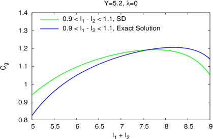
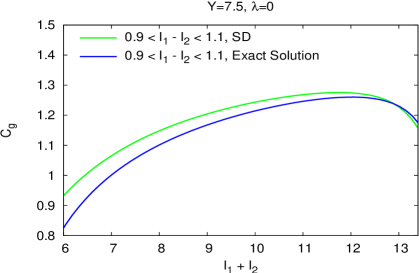
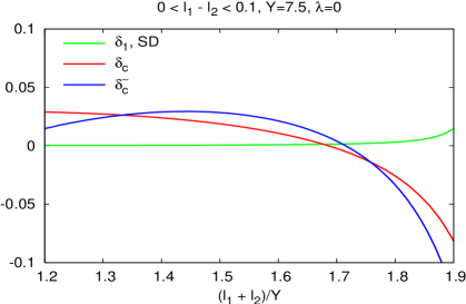
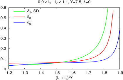
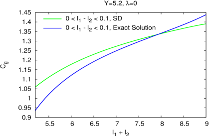
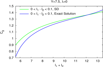
In Figs.8 we compare the SD evaluation of the gluon correlator with the exact solution of [1] at Ξ»=0πœ†0\lambda=0. The difference comes from sub-leading corrections of order Ξ³02superscriptsubscript𝛾02\gamma_{0}^{2} that are not present in (48). For example, βˆ’Ξ²β€‹Ξ³02β‰ˆβˆ’0.2𝛽superscriptsubscript𝛾020.2-\beta\gamma_{0}^{2}\approx-0.2 at Y=5.2π‘Œ5.2Y=5.2 occurring in the exact solution (69) of [1] is not negligible but is absent in (48) and (50). That is why, the SD MLLA curve lies slightly above the one of [1] at small β„“1+β„“2subscriptβ„“1subscriptβ„“2\ell_{1}+\ell_{2}. The mismatch becomes smaller at Y=7.5π‘Œ7.5Y=7.5, since βˆ’Ξ²β€‹Ξ³02β‰ˆβˆ’0.13𝛽superscriptsubscript𝛾020.13-\beta\gamma_{0}^{2}\approx-0.13. However, when β„“1+β„“2subscriptβ„“1subscriptβ„“2\ell_{1}+\ell_{2} increases, the solution of [1] takes over, which can be explained by comparing the behavior of the SD MLLA Ξ΄1subscript𝛿1\delta_{1} obtained in (47) and Ξ΄c,Ξ΄~csubscript𝛿𝑐subscript~𝛿𝑐\delta_{c},\,\tilde{\delta}_{c} in [1]. Namely, while Ξ΄1subscript𝛿1\delta_{1} remains positive and negligible for β„“1β‰ˆβ„“2subscriptβ„“1subscriptβ„“2\ell_{1}\approx\ell_{2}, Ξ΄c,Ξ΄~csubscript𝛿𝑐subscript~𝛿𝑐\delta_{c},\,\tilde{\delta}_{c} decrease and get negative when β„“1+β„“2β†’2​Yβ†’subscriptβ„“1subscriptβ„“22π‘Œ\ell_{1}+\ell_{2}\to 2Y, see Fig.9 (left), which makes the correlations slightly bigger in this region. As |β„“1βˆ’β„“2|subscriptβ„“1subscriptβ„“2|\ell_{1}-\ell_{2}| increases, Ξ΄1subscript𝛿1\delta_{1} is seen in Fig.9 (right) to play the same role as Ξ΄c,Ξ΄~csubscript𝛿𝑐subscript~𝛿𝑐\delta_{c},\tilde{\delta}_{c} do in the solution [1] and therefore, to decrease the correlation. The agreement between both methods improves as the energy scale increases. A similar behavior holds for the quark correlator.
Refer to caption
Refer to caption
Refer to caption
Refer to caption
Figure 8: Comparison between correlators given by SD and in [1], at Ξ»=0πœ†0\lambda=0.
Refer to caption
Refer to caption
Figure 9: Comparison between the SD Ξ΄1subscript𝛿1\delta_{1} and Ξ΄c,Ξ΄~csubscript𝛿𝑐subscript~𝛿𝑐\delta_{c},\,\tilde{\delta}_{c} of [1] at Y=7.5π‘Œ7.5Y=7.5, Ξ»=0πœ†0\lambda=0.

In [1], strong cancellations between the MLLA Ξ΄1subscript𝛿1\delta_{1} and the NMLLA Ξ΄2subscript𝛿2\delta_{2} were seen to take place, giving very small Ξ΄csubscript𝛿𝑐\delta_{c} and Ξ΄~csubscript~𝛿𝑐\tilde{\delta}_{c}; this eased the convergence of the iterative method but raised questions concerning the relative size of MLLA and NMLLA corrections and the validity of the perturbative expansion. However, since Ξ΄1subscript𝛿1\delta_{1} is itself, there, entangled with some NMLLA corrections, no definitive conclusions could be drawn. The present work and Fig.Β 9, by showing that, below, Ξ΄csubscript𝛿𝑐\delta_{c} and Ξ΄~csubscript~𝛿𝑐\tilde{\delta}_{c} of [1] play the same role as the pure MLLA Ξ΄1subscript𝛿1\delta_{1} which is now calculated, suggests (though it is not a demonstration) that the perturbative series is safe. It is indeed compatible with the following scheme: in [1], the pure MLLA part of Ξ΄1subscript𝛿1\delta_{1} is the same as that in the present work; the cancellations in [1] occur between NMLLA corrections included in Ξ΄1subscript𝛿1\delta_{1} and Ξ΄2subscript𝛿2\delta_{2}; these are eventually of the same order of magnitude as MLLA terms, but they are only parts of all NMLLA corrections; this leaves the possibility that the sum of all NMLLA corrections to Ξ΄1subscript𝛿1\delta_{1} and all NMLLA terms of Ξ΄2subscript𝛿2\delta_{2} are separately smaller than the pure MLLA terms of Ξ΄1subscript𝛿1\delta_{1}, that is that strong cancellations occur between NMLLA corrections, the ones included, because of the logic of the calculation, in [1], and those which were not be taken into account.

3.7 Comparison with Fong-Webber and LEP-I data; how 𝝀=πŸŽπ€0\boldsymbol{\lambda=0} is favored

Let us consider, at the Z0superscript𝑍0Z^{0} peak Y=5.2π‘Œ5.2Y=5.2 (Eβ€‹Ξ˜=91.2​GeV​at𝐸Θ91.2GeVatE\Theta=91.2\,\text{GeV}\,\text{at}\,LEP-I energy), the process e+​eβˆ’β†’q​qΒ―β†’superscript𝑒superscriptπ‘’π‘žΒ―π‘že^{+}e^{-}\to q\bar{q}. As can be induced from Fig.8, the results obtained in the present work by the (approximate) SD method are very close to the ones obtained in subsection 6.5 of [1] by the exact solution of the evolution equations. Accordingly, the same comparison as in [1] holds with respect to both Fong & Webber’s results [3] and OPAL data [6].

It is also noticeable that, since, at Ξ»=0πœ†0\lambda=0, correlations already lye above (present) experimental curves, and since an increase of Ξ»πœ†\lambda tends to increase the predictions, the limiting spectrum stays the best candidate to bring agreement with experiments.

4 CONCLUSION

Let us, in a few words, summarize the achievements, but also the limitations of the two methods that have been used respectively in [1] (exact solution of MLLA evolution equations) and in the present work (steepest descent approximate evaluation of their solutions).

Achievements are threefold:
- in [1], MLLA evolution equations for 2-particle correlations have been deduced at small xπ‘₯x and at any Ξ»πœ†\lambda; their (iterative) solution can unfortunately only be expressed analytically at the limit Ξ»β†’0β†’πœ†0\lambda\to 0;
- by the steepest descent method, which is an approximate method, analytical expressions for the spectrum could instead be obtained for Ξ»β‰ 0πœ†0\lambda\neq 0, which enabled to calculate the correlation at the same level of generality;
- one could move away from the peak of the inclusive distribution.

So doing, the limitations of the work of Fong & Webber have vanished. Their results have been recovered at the appropriate limits.

The two methods numerically agree remarkably well, despite an unavoidable entanglement of MLLA + some NMLLA corrections in the first one.

The limitations are the following:
- the uncontrollable increase of Ξ±ssubscript𝛼𝑠\alpha_{s} when one goes to smaller and smaller transverse momenta: improvements in this directions mainly concern the inclusion of non-perturbative contributions;
- departure from the limiting spectrum: it cannot of course appear as a limitation, but we have seen that increasing the value of Ξ»πœ†\lambda, by increasing the correlations, does not bring better agreement with present data; it confirms thus, at present, that the limiting spectrum is the best possibility;
- the LPHD hypothesis: it works surprisingly well for inclusive distributions; only forthcoming data will assert whether its validity decreases when one studies less inclusive processes (like correlations);
- last, the limitation to small xπ‘₯x: it is still quite drastic; departing from this limit most probably lye in the art of numerical calculations, which makes part of forthcoming projects.

Expectations rest on experimental data, which are being collected at the Tevatron, and which will be at LHC. The higher the energy, the safer perturbative QCD is, and the better the agreement should be with our predictions. The remaining disagreement (but much smaller than Fong-Webber’s) between predictions and LEP-1 results for 2-particle correlations stands as an open question concerning the validity of the LPHD hypothesis for these observables which are not β€œso” inclusive as the distributions studied in [5]. The eventual necessity to include NMLLA corrections can only be decided when new data appear.


Acknowledgments:

It is a pleasure to thank Yuri Dokshitzer for enticing me towards the steepest descent method and for showing me its efficiency with simple examples. I am grateful to Bruno Machet for his help and advice and to Gavin Salam for helping me in numerically inverting formula (18a).

Appendix A DOUBLE DERIVATIVES AND DETERMINANT

A.1 Demonstration of eq.Β (20)

We conveniently rewrite (12a) and (12b) in the form

βˆ‚Ο•βˆ‚Ο‰=2β€‹Ο‰βˆ’Ξ½Ο‰βˆ’Ξ½β€‹β„“+Ξ½Ο‰βˆ’Ξ½βˆ’Ο•Ο‰βˆ’Ξ½βˆ’Ξ»β€‹Ξ½+2​s0Ο‰βˆ’Ξ½+1β​ω​(Ο‰βˆ’Ξ½),italic-Ο•πœ”2πœ”πœˆπœ”πœˆβ„“πœˆπœ”πœˆitalic-Ο•πœ”πœˆπœ†πœˆ2subscript𝑠0πœ”πœˆ1π›½πœ”πœ”πœˆ\frac{\partial\phi}{\partial\omega}=\frac{2\omega-\nu}{\omega-\nu}\ell+\frac{\nu}{\omega-\nu}-\frac{\phi}{\omega-\nu}-\lambda\frac{\nu+2s_{0}}{\omega-\nu}+\frac{1}{\beta\omega(\omega-\nu)}, (79)
βˆ‚Ο•βˆ‚Ξ½=Ο‰βˆ’2β€‹Ξ½Ο‰βˆ’Ξ½β€‹yβˆ’Ο‰Ο‰βˆ’Ξ½+Ο•Ο‰βˆ’Ξ½+λ​ω+2​s0Ο‰βˆ’Ξ½βˆ’1β​ν​(Ο‰βˆ’Ξ½).italic-Ο•πœˆπœ”2πœˆπœ”πœˆπ‘¦πœ”πœ”πœˆitalic-Ο•πœ”πœˆπœ†πœ”2subscript𝑠0πœ”πœˆ1π›½πœˆπœ”πœˆ\frac{\partial\phi}{\partial\nu}=\frac{\omega-2\nu}{\omega-\nu}y-\frac{\omega}{\omega-\nu}+\frac{\phi}{\omega-\nu}+\lambda\frac{\omega+2s_{0}}{\omega-\nu}-\frac{1}{\beta\nu(\omega-\nu)}. (80)

The Taylor expansion of (11) in (10) reads

ϕ​(Ο‰,Ξ½,β„“,y)italic-Ο•πœ”πœˆβ„“π‘¦\displaystyle\phi(\omega,\nu,\ell,y)\!\! β‰ˆ\displaystyle\!\!\approx\!\! ϕ​(Ο‰0,Ξ½0,β„“,y)+12β€‹βˆ‚2Ο•βˆ‚Ο‰2​(Ο‰0,Ξ½0)​(Ο‰βˆ’Ο‰0)2+12β€‹βˆ‚2Ο•βˆ‚Ξ½2​(Ο‰0,Ξ½0)​(Ξ½βˆ’Ξ½0)2italic-Ο•subscriptπœ”0subscript𝜈0ℓ𝑦12superscript2italic-Ο•superscriptπœ”2subscriptπœ”0subscript𝜈0superscriptπœ”subscriptπœ”0212superscript2italic-Ο•superscript𝜈2subscriptπœ”0subscript𝜈0superscript𝜈subscript𝜈02\displaystyle\!\!\phi(\omega_{0},\nu_{0},\ell,y)+\frac{1}{2}\,\frac{\partial^{2}\phi}{\partial\omega^{2}}\,(\omega_{0},\nu_{0})(\omega-\omega_{0})^{2}+\frac{1}{2}\,\frac{\partial^{2}\phi}{\partial\nu^{2}}\,(\omega_{0},\nu_{0})(\nu-\nu_{0})^{2} (81)
+βˆ‚2Ο•βˆ‚Ο‰β€‹βˆ‚Ξ½β€‹(Ο‰0,Ξ½0)​(Ο‰βˆ’Ο‰0)​(Ξ½βˆ’Ξ½0).superscript2italic-Ο•πœ”πœˆsubscriptπœ”0subscript𝜈0πœ”subscriptπœ”0𝜈subscript𝜈0\displaystyle+\frac{\partial^{2}\phi}{\partial\omega\partial\nu}(\omega_{0},\nu_{0})\,(\omega-\omega_{0})(\nu-\nu_{0}).

The expressions of the second derivatives follow directly from (79) and (80)

βˆ‚2Ο•βˆ‚Ο‰2=βˆ’Ξ½(Ο‰βˆ’Ξ½)2​(β„“+y+Ξ»)+Ο•(Ο‰βˆ’Ξ½)2βˆ’2β€‹Ο‰βˆ’Ξ½Ξ²β€‹Ο‰2​(Ο‰βˆ’Ξ½)2+4β​(Ο‰βˆ’Ξ½)2​(2​s0+Ο‰+Ξ½),superscript2italic-Ο•superscriptπœ”2𝜈superscriptπœ”πœˆ2β„“π‘¦πœ†italic-Ο•superscriptπœ”πœˆ22πœ”πœˆπ›½superscriptπœ”2superscriptπœ”πœˆ24𝛽superscriptπœ”πœˆ22subscript𝑠0πœ”πœˆ\displaystyle\frac{\partial^{2}\phi}{\partial\omega^{2}}=-\frac{\nu}{(\omega-\nu)^{2}}(\ell\!+\!y\!+\!\lambda)+\frac{\phi}{(\omega-\nu)^{2}}-\frac{2\omega-\nu}{\beta\omega^{2}(\omega-\nu)^{2}}+\frac{4}{\beta(\omega-\nu)^{2}(2s_{0}+\omega+\nu)},
βˆ‚2Ο•βˆ‚Ξ½2=βˆ’Ο‰(Ο‰βˆ’Ξ½)2​(β„“+y+Ξ»)+Ο•(Ο‰βˆ’Ξ½)2+Ο‰βˆ’2​νβ​ν2​(Ο‰βˆ’Ξ½)2+4β​(Ο‰βˆ’Ξ½)2​(2​s0+Ο‰+Ξ½),superscript2italic-Ο•superscript𝜈2πœ”superscriptπœ”πœˆ2β„“π‘¦πœ†italic-Ο•superscriptπœ”πœˆ2πœ”2πœˆπ›½superscript𝜈2superscriptπœ”πœˆ24𝛽superscriptπœ”πœˆ22subscript𝑠0πœ”πœˆ\displaystyle\frac{\partial^{2}\phi}{\partial\nu^{2}}=-\frac{\omega}{(\omega-\nu)^{2}}(\ell\!+\!y\!+\!\lambda)+\frac{\phi}{(\omega-\nu)^{2}}+\frac{\omega-2\nu}{\beta\nu^{2}(\omega-\nu)^{2}}+\frac{4}{\beta(\omega-\nu)^{2}(2s_{0}+\omega+\nu)},
βˆ‚2Ο•βˆ‚Ο‰β€‹βˆ‚Ξ½=Ο‰(Ο‰βˆ’Ξ½)2​(β„“+y+Ξ»)βˆ’Ο•(Ο‰βˆ’Ξ½)2+1β​ω​(Ο‰βˆ’Ξ½)2βˆ’4β​(Ο‰βˆ’Ξ½)2​(2​s0+Ο‰+Ξ½).superscript2italic-Ο•πœ”πœˆπœ”superscriptπœ”πœˆ2β„“π‘¦πœ†italic-Ο•superscriptπœ”πœˆ21π›½πœ”superscriptπœ”πœˆ24𝛽superscriptπœ”πœˆ22subscript𝑠0πœ”πœˆ\displaystyle\frac{\partial^{2}\phi}{\partial\omega\partial\nu}=\frac{\omega}{(\omega-\nu)^{2}}(\ell\!+\!y\!+\!\lambda)-\frac{\phi}{(\omega-\nu)^{2}}+\frac{1}{\beta\omega(\omega-\nu)^{2}}-\frac{4}{\beta(\omega-\nu)^{2}(2s_{0}+\omega+\nu)}.

(10) and its solution can be written in the form

Gβ‰ƒβˆ¬d2​v​eβˆ’12​vT​A​v=2​πD​e​t​Asimilar-to-or-equals𝐺double-integralsuperscript𝑑2𝑣superscript𝑒12superscript𝑣𝑇𝐴𝑣2πœ‹π·π‘’π‘‘π΄G\simeq\iint d^{2}v\,e^{-\frac{1}{2}v^{T}Av}=\frac{2\pi}{\sqrt{Det\,A}}

where

v=(Ο‰,Ξ½),vT=(ων),D​e​t​A=​D​e​t​(βˆ‚2Ο•βˆ‚Ο‰2βˆ‚2Ο•βˆ‚Ο‰β€‹βˆ‚Ξ½βˆ‚2Ο•βˆ‚Ξ½β€‹βˆ‚Ο‰βˆ‚2Ο•βˆ‚Ξ½2)=βˆ‚2Ο•βˆ‚Ο‰2β€‹βˆ‚2Ο•βˆ‚Ξ½2βˆ’(βˆ‚2Ο•βˆ‚Ο‰β€‹βˆ‚Ξ½)2.formulae-sequenceπ‘£πœ”πœˆformulae-sequencesuperscriptπ‘£π‘‡πœ”missing-subexpressionπœˆπ·π‘’π‘‘π΄absent𝐷𝑒𝑑superscript2italic-Ο•superscriptπœ”2superscript2italic-Ο•πœ”πœˆmissing-subexpressionsuperscript2italic-Ο•πœˆπœ”superscript2italic-Ο•superscript𝜈2superscript2italic-Ο•superscriptπœ”2superscript2italic-Ο•superscript𝜈2superscriptsuperscript2italic-Ο•πœ”πœˆ2v=(\omega,\nu),\quad v^{T}=\left(\!\!\begin{array}[]{c}\omega\cr\cr\nu\end{array}\!\!\right),\quad\begin{array}[]{c}DetA=\end{array}Det\left(\begin{array}[]{c}\frac{\partial^{2}\phi}{\partial\omega^{2}}\qquad\frac{\partial^{2}\phi}{\partial\omega\partial\nu}\cr\cr\frac{\partial^{2}\phi}{\partial\nu\partial\omega}\qquad\frac{\partial^{2}\phi}{\partial\nu^{2}}\end{array}\right)=\frac{\partial^{2}\phi}{\partial\omega^{2}}\frac{\partial^{2}\phi}{\partial\nu^{2}}-\left(\frac{\partial^{2}\phi}{\partial\omega\partial\nu}\right)^{2}.

An explicit calculation gives

D​e​t​A=(β„“+y+Ξ»)2​[β​(Ο‰+Ξ½)β€‹Ο•βˆ’4(Ο‰βˆ’Ξ½)2+4​(Ο‰+Ξ½)(Ο‰βˆ’Ξ½)2​(2​s0+Ο‰+Ξ½)]𝐷𝑒𝑑𝐴superscriptβ„“π‘¦πœ†2delimited-[]π›½πœ”πœˆitalic-Ο•4superscriptπœ”πœˆ24πœ”πœˆsuperscriptπœ”πœˆ22subscript𝑠0πœ”πœˆDetA=(\ell+y+\lambda)^{2}\left[\frac{\beta(\omega+\nu)\phi-4}{(\omega-\nu)^{2}}+\frac{4(\omega+\nu)}{(\omega-\nu)^{2}(2s_{0}+\omega+\nu)}\right]

which, by using (16) leads to (20).

A.2 πƒβ€‹πžβ€‹π­β€‹π€πƒπžπ­π€\boldsymbol{DetA} (see eq.Β (20)) around the maximum

This is an addendum to subsection 2.3

β„“m​a​xsubscriptβ„“π‘šπ‘Žπ‘₯\ell_{max} written in (22) is close to the DLA value Y/2π‘Œ2Y/2 [7][8][9]. We then have ΞΌβˆΌΟ…β†’0similar-toπœ‡πœβ†’0\mu\sim\upsilon\to 0 for β„“β‰ˆy≃Y/2ℓ𝑦similar-to-or-equalsπ‘Œ2\ell\approx y\simeq Y/2. In this limit, (18a) and (18b) respectively translate into

Yβˆ’2β€‹β„“β‰ˆΞΌ,Ο…β†’023​(Y+Ξ»)3/2βˆ’Ξ»3/2(Y+Ξ»)1/2​μ,Ο…β‰ˆΞΌ,Ο…β†’0Ξ»Y+λ​μ,formulae-sequencesuperscriptβ†’πœ‡πœ0π‘Œ2β„“23superscriptπ‘Œπœ†32superscriptπœ†32superscriptπ‘Œπœ†12πœ‡superscriptβ†’πœ‡πœ0πœπœ†π‘Œπœ†πœ‡Y-2\ell\stackrel{{\scriptstyle\mu,\upsilon\to 0}}{{\approx}}\frac{2}{3}\,\frac{\left(Y+\lambda\right)^{3/2}-\lambda^{3/2}}{\left(Y+\lambda\right)^{1/2}}\,\mu,\quad\upsilon\stackrel{{\scriptstyle\mu,\upsilon\to 0}}{{\approx}}\sqrt{\frac{\lambda}{Y+\lambda}}\mu, (82)

while

βˆ‚ΞΌβˆ‚β„“β‰ƒβˆ’3​(Y+Ξ»)1/2(Y+Ξ»)3/2βˆ’Ξ»3/2similar-to-or-equalsπœ‡β„“3superscriptπ‘Œπœ†12superscriptπ‘Œπœ†32superscriptπœ†32\frac{\partial\mu}{\partial\ell}\simeq-3\frac{(Y+\lambda)^{1/2}}{(Y+\lambda)^{3/2}-\lambda^{3/2}} (83)

should be used to get (23). An explicit calculation gives

limΞΌ,Ο…β†’0Ξ²1/2​(Y+Ξ»)3/2π​D​e​t​A​(ΞΌ,Ο…)=(3π​β​[(Y+Ξ»)3/2βˆ’Ξ»3/2])1/2,subscriptβ†’πœ‡πœ0superscript𝛽12superscriptπ‘Œπœ†32πœ‹π·π‘’π‘‘π΄πœ‡πœsuperscript3πœ‹π›½delimited-[]superscriptπ‘Œπœ†32superscriptπœ†3212\lim_{\mu,\upsilon\rightarrow 0}\sqrt{\frac{\beta^{1/2}(Y+\lambda)^{3/2}}{\pi DetA(\mu,\upsilon)}}\!=\!\left(\frac{3}{\pi\sqrt{\beta}\left[(Y+\lambda)^{3/2}\!-\!\lambda^{3/2}\right]}\right)^{1/2},

where

D​e​t​A𝐷𝑒𝑑𝐴\displaystyle DetA\! β‰ˆΞΌ,Ο…β†’0superscriptβ†’πœ‡πœ0\displaystyle\!\stackrel{{\scriptstyle\mu,\upsilon\to 0}}{{\approx}}\! β​(Y+Ξ»)3​(ΞΌβˆ’Ο…)​(1+12​μ2)​(1+12​υ2)+(1+12​μ2)​(Ο…+16​υ3)βˆ’(ΞΌ+16​μ3)​(1+12​υ2)ΞΌ3𝛽superscriptπ‘Œπœ†3πœ‡πœ112superscriptπœ‡2112superscript𝜐2112superscriptπœ‡2𝜐16superscript𝜐3πœ‡16superscriptπœ‡3112superscript𝜐2superscriptπœ‡3\displaystyle\!\beta(Y\!+\!\lambda)^{3}\frac{\left(\mu\!-\!\upsilon\right)\left(1\!+\!\frac{1}{2}\mu^{2}\right)\left(1\!+\!\frac{1}{2}\upsilon^{2}\right)\!+\!(1\!+\!\frac{1}{2}\mu^{2})\left(\upsilon\!+\!\frac{1}{6}\upsilon^{3}\right)\!-\!\left(\mu\!+\!\frac{1}{6}\mu^{3}\right)\left(1\!+\!\frac{1}{2}\upsilon^{2}\right)}{\mu^{3}} (84)
≃similar-to-or-equals\displaystyle\!\simeq\! 13​β​(Y+Ξ»)3​(1βˆ’Ο…3ΞΌ3)=13​β​(Y+Ξ»)3​[1βˆ’(Ξ»Y+Ξ»)3/2].13𝛽superscriptπ‘Œπœ†31superscript𝜐3superscriptπœ‡313𝛽superscriptπ‘Œπœ†3delimited-[]1superscriptπœ†π‘Œπœ†32\displaystyle\!\frac{1}{3}\beta(Y\!+\!\lambda)^{3}\left(1\!-\!\frac{\upsilon^{3}}{\mu^{3}}\right)=\frac{1}{3}\beta(Y+\lambda)^{3}\left[1-\left(\frac{\lambda}{Y+\lambda}\right)^{3/2}\right].

A.3 The functions 𝐋​(𝛍,𝛖)𝐋𝛍𝛖\boldsymbol{L(\mu,\upsilon)}, πŠβ€‹(𝛍,𝛖)πŠπ›π›–\boldsymbol{K(\mu,\upsilon)} in eq.Β (30)

An explicit calculation gives

L​(ΞΌ,Ο…)=32​cosh⁑μsinhβ‘ΞΌβˆ’12​(ΞΌβˆ’Ο…)​cosh⁑υ​sinh⁑μ+sinh⁑υ​sinh⁑μ(ΞΌβˆ’Ο…)​cosh⁑μ​cosh⁑υ+cosh⁑μ​sinhβ‘Ο…βˆ’sinh⁑μ​cosh⁑υ,πΏπœ‡πœ32πœ‡πœ‡12πœ‡πœπœπœ‡πœπœ‡πœ‡πœπœ‡πœπœ‡πœπœ‡πœL(\mu,\upsilon)=\frac{3}{2}\frac{\cosh\mu}{\sinh\mu}-\frac{1}{2}\frac{(\mu-\upsilon)\cosh\upsilon\sinh\mu+\sinh\upsilon\sinh\mu}{(\mu-\upsilon)\cosh\mu\cosh\upsilon+\cosh\mu\sinh\upsilon-\sinh\mu\cosh\upsilon}, (85)

and

K​(ΞΌ,Ο…)=βˆ’12​sinh⁑υ​(ΞΌβˆ’Ο…)​coshβ‘ΞΌβˆ’sinh⁑μ(ΞΌβˆ’Ο…)​cosh⁑μ​cosh⁑υ+cosh⁑μ​sinhβ‘Ο…βˆ’sinh⁑μ​cosh⁑υ.πΎπœ‡πœ12πœπœ‡πœπœ‡πœ‡πœ‡πœπœ‡πœπœ‡πœπœ‡πœK(\mu,\upsilon)=-\frac{1}{2}\sinh\upsilon\frac{(\mu-\upsilon)\cosh\mu-\sinh\mu}{(\mu-\upsilon)\cosh\mu\cosh\upsilon+\cosh\mu\sinh\upsilon-\sinh\mu\cosh\upsilon}. (86)

A.4 A consistency check

Let us verify that the evolution equation (2) is satisfied by (21) within the MLLA accuracy. Differentiating (2) with respect to β„“β„“\ell, y𝑦y yields the equivalent differential equation

Gℓ​y=Ξ³02​(Gβˆ’a​Gβ„“)+π’ͺ​(Ξ³04​G)subscript𝐺ℓ𝑦superscriptsubscript𝛾02πΊπ‘Žsubscript𝐺ℓπ’ͺsuperscriptsubscript𝛾04𝐺G_{\ell y}=\gamma_{0}^{2}\left(G-aG_{\ell}\right)\!+\!{\cal{O}}{\big{(}\gamma_{0}^{4}G\big{)}}

that can be rewritten in the form

Οˆβ„“β€‹Οˆy+Οˆβ„“β€‹y=Ξ³02​(1βˆ’aβ€‹Οˆβ„“)+π’ͺ​(Ξ³04);subscriptπœ“β„“subscriptπœ“π‘¦subscriptπœ“β„“π‘¦superscriptsubscript𝛾021π‘Žsubscriptπœ“β„“π’ͺsuperscriptsubscript𝛾04\psi_{\ell}\psi_{y}+\psi_{\ell y}\>=\>\gamma_{0}^{2}\left(1-a\psi_{\ell}\right)\>+\>{\cal{O}}\big{(}{\gamma_{0}^{4}}\big{)}; (87)

we have neglected next-to-MLLA corrections π’ͺ​(Ξ³04)π’ͺsuperscriptsubscript𝛾04{\cal O}(\gamma_{0}^{4}) (of relative order Ξ³02superscriptsubscript𝛾02\gamma_{0}^{2}) coming from differentiating the coupling Ξ³02superscriptsubscript𝛾02\gamma_{0}^{2} in the sub-leading (β€œhard correction”) term ∝aproportional-toabsentπ‘Ž\propto a.

We have to make sure that (87) holds including the terms π’ͺ​(Ξ³03)π’ͺsuperscriptsubscript𝛾03{\cal O}(\gamma_{0}^{3}). In the sub-leading terms we can set Οˆβ†’Ο†β†’πœ“πœ‘\psi\to\varphi (see (26)):

(Ο†β„“+Ξ΄β€‹Οˆβ„“)​(Ο†y+Ξ΄β€‹Οˆy)+φℓ​y=Ξ³02​(1βˆ’a​φℓ).subscriptπœ‘β„“π›Ώsubscriptπœ“β„“subscriptπœ‘π‘¦π›Ώsubscriptπœ“π‘¦subscriptπœ‘β„“π‘¦superscriptsubscript𝛾021π‘Žsubscriptπœ‘β„“(\varphi_{\ell}+\delta\psi_{\ell})(\varphi_{y}+\delta\psi_{y})+\varphi_{\ell y}=\gamma_{0}^{2}(1-a\varphi_{\ell}). (88)

Isolating correction terms and casting them all on the l.h.s. of the equation we get

a​γ02​φℓ+[Ο†β„“β€‹Ξ΄β€‹Οˆy+Ο†yβ€‹Ξ΄β€‹Οˆβ„“]+φℓ​y=Ξ³02βˆ’Ο†β„“β€‹Ο†y.π‘Žsuperscriptsubscript𝛾02subscriptπœ‘β„“delimited-[]subscriptπœ‘β„“π›Ώsubscriptπœ“π‘¦subscriptπœ‘π‘¦π›Ώsubscriptπœ“β„“subscriptπœ‘β„“π‘¦superscriptsubscript𝛾02subscriptπœ‘β„“subscriptπœ‘π‘¦a\gamma_{0}^{2}\varphi_{\ell}+\left[\,\varphi_{\ell}\delta\psi_{y}+\varphi_{y}\delta\psi_{\ell}\,\right]+\varphi_{\ell y}\>=\>\gamma_{0}^{2}-\varphi_{\ell}\varphi_{y}. (89)

By the definition (26) of the saddle point we conclude that the r.h.s. of (89) is zero such that we have

Ο‰0​a​γ02+[Ο‰0β€‹Ξ΄β€‹Οˆy+Ξ½0β€‹Ξ΄β€‹Οˆβ„“]+d​ω0d​y=β€…0,subscriptπœ”0π‘Žsuperscriptsubscript𝛾02delimited-[]subscriptπœ”0𝛿subscriptπœ“π‘¦subscript𝜈0𝛿subscriptπœ“β„“π‘‘subscriptπœ”0𝑑𝑦 0\omega_{0}a\gamma_{0}^{2}+\left[\,\omega_{0}\delta\psi_{y}+\nu_{0}\delta\psi_{\ell}\,\right]+\frac{d\omega_{0}}{dy}\>=\>0\,, (90)

that is,

Ο‰0​(a​γ02+Ξ΄β€‹Οˆy)+Ξ½0β€‹Ξ΄β€‹Οˆβ„“+d​ω0d​y=β€…0.subscriptπœ”0π‘Žsuperscriptsubscript𝛾02𝛿subscriptπœ“π‘¦subscript𝜈0𝛿subscriptπœ“β„“π‘‘subscriptπœ”0𝑑𝑦 0\omega_{0}\left(a\gamma_{0}^{2}+\delta\psi_{y}\right)+\nu_{0}\delta\psi_{\ell}+\frac{d\omega_{0}}{dy}\>=\>0\,. (91)

First, we select the terms ∝aproportional-toabsentπ‘Ž\propto a:

aΞ³03[βˆ’12Q~βˆ’12tanhΟ…eΞΌ+12tanhΟ…cothΞΌeΞΌ+12tanhΟ…cothΞΌQ~\displaystyle a\gamma_{0}^{3}\left[-\frac{1}{2}\widetilde{Q}-\frac{1}{2}\tanh\upsilon\,e^{\mu}+\frac{1}{2}\tanh\upsilon\coth\mu\,e^{\mu}+\frac{1}{2}\tanh\upsilon\coth\mu\,\widetilde{Q}\right.
+12Q~βˆ’12tanhΟ…eβˆ’ΞΌβˆ’12tanhΟ…cothΞΌeβˆ’ΞΌβˆ’12tanhΟ…cothΞΌQ~]\displaystyle\left.+\frac{1}{2}\widetilde{Q}-\frac{1}{2}\tanh\upsilon\,e^{-\mu}-\frac{1}{2}\tanh\upsilon\coth\mu\,e^{-\mu}-\frac{1}{2}\tanh\upsilon\coth\mu\,\widetilde{Q}\right]
=a​γ03​[βˆ’tanh⁑υ​cosh⁑μ+tanh⁑υ​coth⁑μ​sinh⁑μ]≑0.absentπ‘Žsuperscriptsubscript𝛾03delimited-[]πœπœ‡πœhyperbolic-cotangentπœ‡πœ‡0\displaystyle=a\gamma_{0}^{3}\left[-\tanh\upsilon\cosh\mu+\tanh\upsilon\coth\mu\sinh\mu\right]\equiv 0.

From (16) one deduces

d​ω0d​y=12​β​γ03​Q~,𝑑subscriptπœ”0𝑑𝑦12𝛽superscriptsubscript𝛾03~𝑄\frac{d\omega_{0}}{dy}=\frac{1}{2}\beta\gamma_{0}^{3}\widetilde{Q},

that is inserted in (91) such that, for terms ∝βproportional-toabsent𝛽\propto\beta, we have

βˆ’Ξ²Ξ³03[12eΞΌ+12tanhΟ…(1+K)eΞΌβˆ’12CeΞΌβˆ’12CQ~+12eβˆ’ΞΌ+12tanhΟ…(1+K)eβˆ’ΞΌ\displaystyle-\beta\gamma_{0}^{3}\left[\frac{1}{2}e^{\mu}+\frac{1}{2}\tanh\upsilon\Big{(}1\!+\!K\Big{)}e^{\mu}-\frac{1}{2}C\,e^{\mu}-\frac{1}{2}C\widetilde{Q}+\frac{1}{2}e^{-\mu}+\frac{1}{2}\tanh\upsilon\Big{(}1\!+\!K\Big{)}e^{-\mu}\right.
+12Ceβˆ’ΞΌ+12CQ~]=βˆ’Ξ²Ξ³03[coshΞΌ+tanhΟ…coshΞΌ(1+K)βˆ’CsinhΞΌβˆ’12Q~],\displaystyle\left.+\frac{1}{2}C\,e^{-\mu}+\frac{1}{2}C\widetilde{Q}\right]=-\beta\gamma_{0}^{3}\left[\cosh\mu+\tanh\upsilon\cosh\mu\Big{(}1\!+\!K\Big{)}-C\sinh\mu-\frac{1}{2}\widetilde{Q}\right],

which gives

βˆ’Ξ²β€‹Ξ³03​[coshβ‘ΞΌβˆ’sinh⁑μ​Lβˆ’12​Q~].𝛽superscriptsubscript𝛾03delimited-[]πœ‡πœ‡πΏ12~𝑄\displaystyle-\beta\gamma_{0}^{3}\left[\cosh\mu-\sinh\mu\,L-\frac{1}{2}\widetilde{Q}\right].

Constructing (see (33) and appendix A.3)

Q~​(ΞΌ,Ο…)βˆ’2​cosh⁑μ~π‘„πœ‡πœ2πœ‡\displaystyle\widetilde{Q}(\mu,\upsilon)-2\cosh\mu\!\! =\displaystyle\!\!=\!\! βˆ’3​cosh⁑μ+sinh⁑μ​(ΞΌβˆ’Ο…)​cosh⁑υ​sinh⁑μ+sinh⁑υ​sinh⁑μ(ΞΌβˆ’Ο…)​cosh⁑μ​cosh⁑υ+cosh⁑μ​sinhβ‘Ο…βˆ’sinh⁑μ​cosh⁑υ3πœ‡πœ‡πœ‡πœπœπœ‡πœπœ‡πœ‡πœπœ‡πœπœ‡πœπœ‡πœ\displaystyle\!\!-3\cosh\mu+\sinh\mu\frac{(\mu-\upsilon)\cosh\upsilon\sinh\mu+\sinh\upsilon\sinh\mu}{(\mu-\upsilon)\cosh\mu\cosh\upsilon+\cosh\mu\sinh\upsilon-\sinh\mu\cosh\upsilon}
=\displaystyle\!\!=\!\! βˆ’2​sinh⁑μ​L​(ΞΌ,Ο…)2πœ‡πΏπœ‡πœ\displaystyle\!\!-2\sinh\mu L(\mu,\upsilon)

we have

βˆ’Ξ²β€‹Ξ³03​[coshβ‘ΞΌβˆ’sinh⁑μ​Lβˆ’12​Q~]≑0.𝛽superscriptsubscript𝛾03delimited-[]πœ‡πœ‡πΏ12~𝑄0-\beta\gamma_{0}^{3}\left[\cosh\mu-\sinh\mu\,L-\frac{1}{2}\widetilde{Q}\right]\equiv 0.

Appendix B ANALYTICAL EXPRESSION OF πš«β€²β€‹(π›πŸ,π›πŸ)superscript𝚫bold-β€²subscript𝛍1subscript𝛍2\boldsymbol{\Delta^{\prime}(\mu_{1},\mu_{2})} OBTAINED FROM EQ.Β (45)

Replacing (34c)(34f) in (45) and neglecting terms of relative order π’ͺ​(Ξ³03)π’ͺsuperscriptsubscript𝛾03{\cal O}(\gamma_{0}^{3}) which are beyond the MLLA accuracy, we obtain

Ξ”β€²superscriptΞ”β€²\displaystyle\Delta^{\prime}\!\! =\displaystyle\!\!=\!\! eβˆ’ΞΌ1β€‹Ξ΄β€‹Οˆ2,β„“+eβˆ’ΞΌ2β€‹Ξ΄β€‹Οˆ1,β„“+eΞΌ1β€‹Ξ΄β€‹Οˆ2,y+eΞΌ2β€‹Ξ΄β€‹Οˆ1,yΞ³0superscript𝑒subscriptπœ‡1𝛿subscriptπœ“2β„“superscript𝑒subscriptπœ‡2𝛿subscriptπœ“1β„“superscript𝑒subscriptπœ‡1𝛿subscriptπœ“2𝑦superscript𝑒subscriptπœ‡2𝛿subscriptπœ“1𝑦subscript𝛾0\displaystyle\!\!\frac{e^{-\mu_{1}}\delta\psi_{2,\ell}+e^{-\mu_{2}}\delta\psi_{1,\ell}+e^{\mu_{1}}\delta\psi_{2,y}+e^{\mu_{2}}\delta\psi_{1,y}}{\gamma_{0}} (92)
=\displaystyle\!\!=\!\! βˆ’aΞ³0[eΞΌ1+eΞΌ2βˆ’sinh(ΞΌ1βˆ’ΞΌ2)(Q~1βˆ’Q~2)+coshΞΌ1tanhΟ…2+coshΞΌ2tanhΟ…1\displaystyle\!\!-a\gamma_{0}\left[e^{\mu_{1}}+e^{\mu_{2}}-\sinh(\mu_{1}-\mu_{2})(\widetilde{Q}_{1}-\widetilde{Q}_{2})+\cosh\mu_{1}\tanh\upsilon_{2}+\cosh\mu_{2}\tanh\upsilon_{1}\right. (102)
βˆ’sinh⁑μ1​tanh⁑υ2​coth⁑μ2βˆ’sinh⁑μ2​tanh⁑υ1​coth⁑μ1subscriptπœ‡1subscript𝜐2hyperbolic-cotangentsubscriptπœ‡2subscriptπœ‡2subscript𝜐1hyperbolic-cotangentsubscriptπœ‡1\displaystyle\hskip 28.45274pt\left.-\sinh\mu_{1}\tanh\upsilon_{2}\coth\mu_{2}-\sinh\mu_{2}\tanh\upsilon_{1}\coth\mu_{1}\right.
+sinh(ΞΌ1βˆ’ΞΌ2)(tanhΟ…1cothΞΌ1Q~1βˆ’tanhΟ…2cothΞΌ2Q~2)]\displaystyle\hskip 28.45274pt\left.+\sinh(\mu_{1}-\mu_{2})\Big{(}\tanh\upsilon_{1}\coth\mu_{1}\widetilde{Q}_{1}-\tanh\upsilon_{2}\coth\mu_{2}\widetilde{Q}_{2}\Big{)}\right]
βˆ’Ξ²Ξ³0[(coshΞΌ1βˆ’sinhΞΌ1C2)+(coshΞΌ2βˆ’sinhΞΌ2C1)+sinh(ΞΌ1βˆ’ΞΌ2)(C1Q~1βˆ’C2Q~2)\displaystyle-\beta\gamma_{0}\left[\Big{(}\cosh\mu_{1}-\sinh\mu_{1}C_{2}\Big{)}+\Big{(}\cosh\mu_{2}-\sinh\mu_{2}C_{1}\Big{)}+\sinh(\mu_{1}-\mu_{2})(C_{1}\widetilde{Q}_{1}-C_{2}\widetilde{Q}_{2})\right.
+coshΞΌ1tanhΟ…2(1+K2)+coshΞΌ2tanhΟ…1(1+K1)].\displaystyle\hskip 28.45274pt\left.+\cosh\mu_{1}\tanh\upsilon_{2}\Big{(}1+K_{2}\Big{)}+\cosh\mu_{2}\tanh\upsilon_{1}\Big{(}1+K_{1}\Big{)}\right].


References

  • [1] R. Perez-Ramos: JHEP 06 (2006) 019, hep-ph/0605083, and references therein.
  • [2] Yu.L. Dokshitzer, V.A. Khoze and S.I. Troyan: Int. J. Mod. Phys. A7 (1992) 1875.
  • [3] C.P. Fong and B.R. Webber: Phys. Lett. B 241 (1990) 255.
  • [4] Yu.L. Dokshitzer, V.A. Khoze, S.I. Troyan and A.H. Mueller: Rev. Mod. Phys. 60 (1988) 373-388.
  • [5] R. Perez-Ramos & B. Machet: JHEP 04 (2006) 043, hep-ph/0512236.
  • [6] OPAL Collab.: Phys. Lett. B 287 (1992) 401.
  • [7] Yu.L. Dokshitzer, V.S. Fadin and V.A. Khoze: Z. Phys C18 (1983) 37.
  • [8] Yu.L. Dokshitzer, V.A. Khoze, A.H. Mueller and S.I. Troyan: β€œBasics of Perturbative QCD”, Editions FrontiΓ¨res, Paris, 1991.
  • [9] V.A. Khoze and W. Ochs: Int. J. Mod. Phys. A12 (1997) 2949.
  • [10] C.P. Fong and B.R. Webber: Phys. Lett. B 229 (1989) 289.