DESY 05–012 hep-ph/0607200

SFB-CPP-06/33

Non–Singlet QCD Analysis of Deep Inelastic

World Data at $O(\alpha_{s}^{3})$

Johannes Blümlein^a, Helmut Böttcher^a,b, and Alberto Guffanti^a

^aDeutsches Elektronen Synchrotron, DESY

Platanenallee 6, D–15738 Zeuthen, Germany

^bInstitut für Physik, Humboldt–Universität, Newtonstraße. 15, D–12489 Berlin

A non–singlet QCD analysis of the structure function $F_{2}(x,q^{2})$ in LO, NLO, NNLO and N³LO is performed based on the world data for charged lepton scattering. We determine the valence quark parton densities and present their parameterization and that of the correlated errors in a wide range of $x$ and $Q^{2}$. In the analysis we determined the QCD–scale $\Lambda_{\rm QCD,N_{f}=4}^{\overline{\rm MS}}=265\pm 27\,\mbox{MeV}~{}~{}{\rm(NLO)},~{}~{}226\pm 25\,\mbox{MeV}~{}~{}{\rm(NNLO)},~{}~{}234\pm 26\,\mbox{MeV}~{}~{}{\rm(N^{3}LO)}$, with a remainder uncertainty of $\pm 2\,\mbox{MeV}$ for the yet unknown 4–loop anomalous dimension, corresponding to $\alpha_{s}(M_{Z}^{2})=0.1148\pm 0.0019~{}~{}{\rm NLO},~{}~{}0.1134{\tiny{\begin{array}[]{c}+0.0019\\ -0.0021\end{array}}}~{}~{}{\rm NNLO},~{}~{}0.1141{\tiny{\begin{array}[]{c}+0.0020\\ -0.0022\end{array}}}~{}~{}{\rm N^{3}LO}$. A comparison is performed to other determinations of the QCD scale and $\alpha_{s}(M_{Z}^{2})$ in deeply inelastic scattering. The higher twist contributions of $F_{2}^{p}(x,Q^{2})$ and $F_{2}^{d}(x,Q^{2})$ are extracted in the large $x$ region, subtracting the twist–2 contributions obtained in the NLO, NNLO and N³LO analysis.

1 Introduction

Deeply inelastic scattering (DIS) at large 4–momentum transfer $Q^{2}=-q^{2}$ offers the possibility to probe the partonic sub–structure of the nucleon. The light–cone expansion [1] allows to describe the forward Compton amplitude in terms of the twist–expansion. For the twist–2 contributions the factorization theorems hold and the calculation of the scaling violations of the parton distribution functions and structure functions is possible within the framework of perturbative Quantum Chromodynamics (QCD). In the present paper we determine the flavor non–singlet parton distribution functions $xu_{v}(x,Q^{2})$ and $xd_{v}(x,Q^{2})$ using the available $e(\mu)p$ and $e(\mu)d$ world data [2, 3, 4, 5, 6] up to the next-to-next-to leading (NNLO) and next-to-next-to-next to leading order level (N³LO). This is possible due to the advent of the 3–loop non–singlet anomalous dimensions [7] and 3–loop Wilson coefficients [8], as well as first informations on the 4–loop non–singlet anomalous dimension, with its second moment [10]. The QCD analysis of the world non–singlet data has the advantage to deal with a restricted set of parton distribution functions, to which the virtual photon couples directly and which do therefore contribute already at leading order. The analysis is, furthermore, free of assumptions on the gluon distribution function which stabilizes the systematics since a lower number of parameters describing the parton distributions has to be measured and the analysis is free of the correlation between the QCD scale $\Lambda_{\rm QCD}$ and the gluon density. Also due to the particular behaviour of the flavor non–singlet parton densities in the smaller Bjorken–$x$ region in comparison to the sea–quark and gluon densities a separate non–singlet analysis is in order to better understand systematics effects present in combined non–singlet and singlet analyses.

Previous 3–loop QCD analyses were mainly performed as combined singlet and non–singlet analyses [11, 12], partly based on preliminary, approximative expression of the 3–loop splitting functions. Other analyses were carried out for fixed moments only in the singlet [14, 15] and non-singlet case analyzing neutrino data [14]. First results of our non–singlet analysis were published in [17]. Very recently a 3–loop non–singlet analysis was also carried out in Ref. [18]. There are numerous NLO analyses, among them [2, 5, 6, 19], which we will use in comparisons below. Another recent NLO parameterization [20] fixes $\alpha_{s}(M_{Z}^{2})$ and presents a series of ten parton distribution sets associated to equidistant values of the strong coupling constant in the range $\alpha_{s}(M_{Z}^{2})~{}\epsilon~{}[0.110,~{}0.128]$.

The non-singlet analysis will provide us with the distribution functions $xu_{v}(x,Q^{2})$ and $xd_{v}(x,Q^{2})$ with correlated errors. From these distributions we may form Mellin–moments which can be compared to lattice–simulations of these quantities. The lattice calculations have to be performed at as low as possible pion masses due to a potential non–linear behaviour on $m_{\pi}$ in the small mass region and non–perturbative renormalization has to be used. Precision results of these simulations with $N_{f}=2$ dynamical quarks are expected soon. The comparison of the Mellin moments obtained in a 3(4)–loop QCD analysis of the non–singlet World Data at the one side and lattice simulations on the other side will lead to new important tests of Quantum Chromodynamics.

The paper is organized as follows. In Section 2 we briefly summarize the basic formalism. The data analysis and calculation of errors is outlined in Section 3. Different corrections such as the account for a finite sea quark difference $x(\overline{d}-\overline{u})(x,Q^{2})$, heavy quark contributions, target mass and deuteron wave function corrections are dealt with in Section 4. The fit results for the non–singlet parton distribution functions, their correlated errors and evolution are presented in Section 5, where also comparisons to other analyses are made. In Section 6 the results on $\Lambda_{\rm QCD}$ and $\alpha_{s}(M_{Z}^{2})$ in NLO, NNLO and N³LO are given and compared to other NLO and NNLO results. In Section 7 we present our results on the higher twist contributions in the large $x$ region for the structure functions $F_{2}^{p}(x,Q^{2})$ and $F_{2}^{d}(x,Q^{2})$ and Section 8 contains the conclusions.

2 Basic Formalism

We choose the following parameterization for the valence quark densities

$$xv_{i}(x,Q^{2})=A_{i}x^{a_{i}}(1-x)^{b_{i}}(1+\rho_{i}\sqrt{x}+\gamma_{i}x)~{},$$ (1)

with $v_{i}=u_{v},d_{v},~{}i=u,d$. Three valence–projections are considered. In the region $x\leq 0.3$ for the difference of the proton and deuteron data we use

$$f^{\rm NS}(x,Q^{2})=\frac{1}{3}\left[x(u+\overline{u})(x,Q^{2})-x(d+\overline{d})(x,Q^{2})\right]~{}.$$ (2)

The combinations of parton densities in the valence region $x>0.3$ for $F_{2}^{p,d}(x,Q^{2})$ are

$$f^{v}_{p}(x,Q^{2}) = \frac{5}{18}\left[x(u-\overline{u})(x,Q^{2})+x(d-\overline{d})(x,Q^{2})\right]+\frac{1}{6}\left[x(u-\overline{u})(x,Q^{2})-x(d-\overline{d})(x,Q^{2})\right]$$

$$f^{v}_{d}(x,Q^{2}) = \frac{5}{18}\left[x(u-\overline{u})(x,Q^{2})+x(d-\overline{d})(x,Q^{2})\right]~{}.$$ (4)

The evolution equations are solved in Mellin-$N$ space and the Mellin transforms of the above distributions are denoted by $f^{\rm NS}(N,Q^{2}),f^{v}_{p,d}(N,Q^{2})$, respectively. The non–singlet structure functions are given by

$$F_{k}(N,Q^{2})=\left[1+a_{s}(Q^{2})C_{1}(N)+a_{s}^{2}(Q^{2})C_{2}(N)+a_{s}^{3}(Q^{2})C_{3}(N)\right]f_{k}(N,Q^{2})$$ (5)

for the three cases above. Here $a_{s}(Q^{2})=\alpha_{s}(Q^{2})/(4\pi)$ denotes the strong coupling constant and $C_{i}(N)(Q^{2})$ are the non–singlet Wilson coefficients in $O(a_{s}^{i})$ [21, 22, 8]. For the representation of the Wilson coefficients we used those given in [23, 8] which are based on numerical fits. For the 2–loop Wilson coefficients and 3–loop anomalous dimensions compact analytic representations are also available, based on the reduction of the respective harmonic sums to 5 (14) basic functions [24, 25, 26, 27, 28].

The solution of the non–singlet evolution equation for the parton densities to 4–loop order reads

$$F_{k}(N,Q^{2}) = F_{k}(N,Q_{0}^{2})\left(\frac{a}{a_{0}}\right)^{-\hat{P}_{0}(N)/{\beta_{0}}}\Biggl{\{}1-\frac{1}{\beta_{0}}(a-a_{0})\left[\hat{P}_{1}^{+}(N)-\frac{\beta_{1}}{\beta_{0}}\hat{P}_{0}\right]$$ (6)

$$-\frac{1}{2\beta_{0}}\left(a^{2}-a_{0}^{2}\right)\left[\hat{P}_{2}^{+}(N)-\frac{\beta_{1}}{\beta_{0}}\hat{P}_{1}^{+}+\left(\frac{\beta_{1}^{2}}{\beta_{0}^{2}}-\frac{\beta_{2}}{\beta_{0}}\right)\hat{P}_{0}(N)\right]$$

$$+\frac{1}{2\beta_{0}^{2}}\left(a-a_{0}\right)^{2}\left(\hat{P}_{1}^{+}(N)-\frac{\beta_{1}}{\beta_{0}}\hat{P}_{0}\right)^{2}$$

$$-\frac{1}{3\beta_{0}}\left(a^{3}-a_{0}^{3}\right)\Biggl{[}\hat{P}_{3}^{+}(N)-\frac{\beta_{1}}{\beta_{0}}\hat{P}_{2}^{+}(N)+\left(\frac{\beta_{1}^{2}}{\beta_{0}^{2}}-\frac{\beta_{2}}{\beta_{0}}\right)\hat{P}_{1}^{+}(N)$$

$$+\left(\frac{\beta_{1}^{3}}{\beta_{0}^{3}}-2\frac{\beta_{1}\beta_{2}}{\beta_{0}^{2}}+\frac{\beta_{3}}{\beta_{0}}\right)\hat{P}_{0}(N)\Biggr{]}$$

$$+\frac{1}{2\beta_{0}^{2}}\left(a-a_{0}\right)\left(a_{0}^{2}-a^{2}\right)\left(\hat{P}_{1}^{+}(N)-\frac{\beta_{1}}{\beta_{0}}\hat{P}_{0}(N)\right)$$

$$\times\left[\hat{P}_{2}(N)-\frac{\beta_{1}}{\beta_{0}}\hat{P}_{1}(N)-\left(\frac{\beta_{1}^{2}}{\beta_{0}^{2}}-\frac{\beta_{2}}{\beta_{0}}\right)\hat{P}_{0}(N)\right]$$

$$-\frac{1}{6\beta_{0}^{3}}\left(a-a_{0}\right)^{3}\left(\hat{P}_{1}^{+}(N)-\frac{\beta_{1}}{\beta_{0}}\hat{P}_{0}(N)\right)^{3}\Bigg{\}}~{}.$$

Here, $\hat{P}_{k}$ denote the Mellin transforms of the $(k+1)$–loop splitting functions.

The strong coupling constant obeys the evolution equation

$$\frac{da_{s}(Q^{2})}{d\ln Q^{2}}=-\sum_{k=0}^{\infty}\beta_{k}a_{s}^{k+2}(Q^{2})~{}.$$ (7)

Eq. (7) is solved in the $\overline{\rm MS}$–scheme applying the matching of flavor thresholds at $Q^{2}=m_{c}^{2}$ and $Q^{2}=m_{b}^{2}$ with $m_{c}=1.5\,\mbox{GeV}$ and $m_{b}=4.5\,\mbox{GeV}$ as described in [31, 32]. The convention for the $\overline{\rm MS}$–scheme introduced in [33] is extended in this way. To be capable to compare with other measurements of $\Lambda_{\rm QCD}$ we adopt this prescription.

3 Data Analysis and Error Calculation

For the non–singlet QCD analysis presented in the present paper structure function data measured in charged lepton proton and deuteron deep inelastic scattering are used. The experiments contributing to the statistics are BCDMS [2], SLAC [3], NMC [4], H1 [5], and ZEUS [6]. The BCDMS data were recalculated replacing $R_{QCD}$ by $R_{1998}$ [34]. The SLAC data come from a re-analysis of the data from the experiments E49, E61, E87, and E89. All deuteron data were corrected for Fermi motion and off-shell effects [35]. We form three data samples : $F_{2}^{p}(x,Q^{2})$, $F_{2}^{d}(x,Q^{2})$ in the valence quark region $x\geq 0.3$ and $F_{2}^{NS}=2(F_{2}^{p}-F_{2}^{d})$ in the region $x<0.3$. In the valence quark region we approximate the parton distribution functions by pure valence quarks. Only data with $Q^{2}>4~{}\,\mbox{GeV}^{2}$ were included in the analysis and a cut in the hadronic mass of $W^{2}>12.5~{}\,\mbox{GeV}^{2}$ was applied in order to widely eliminate higher twist effects from the data samples. After these cuts we are left with 762 data points, 322 for $F_{2}^{p}$, 232 for $F_{2}^{d}$, and 208 for $F_{2}^{NS}$. The BCDMS data have been used with an additional cut of $y_{\mu}>0.3$ in order to exclude a region with significant correlated systematic errors, cf. also [5]. In case of $e(\mu)N$ deep inelastic scattering experiments measuring the kinematic variables either only form the lepton or the outgoing jet–kinematics the systematics of the respective measurement becomes worse at low values of $y$ (lepton measurement) or high values of $y$ (jet measurement). These effects were studied in Ref. [36] and give rise to the $y$–cut mentioned for the BCDMS-data. A cut of $Q^{2}>8~{}{\rm\,\mbox{GeV}^{2}}$ was imposed on the NMC data. These cuts reduce the total number of data points available for the analysis from 762 to 551.

The data sets used contain both statistical and systematic errors which in turn, for some data sets, split into uncorrelated and correlated ones. There are several procedures proposed to treat the experimental errors and the determination of uncertainties from parton distributions [37]. Here we decided to use the simplest procedure by adding the statistical and systematic errors, uncorrelated and correlated ones, in quadrature when using the data sets in the fit. However, we allowed for a relative normalization shift $N_{i}$ between the different data sets within the normalization uncertainties $\Delta N_{i}$ quoted by the experiments or assumed accordingly. These normalization shifts were fitted once and then kept fixed. The number of data points, their $x$ and $Q^{2}$ range, and the normalization shifts determined are summarized in Table 1.

The normalization shift for each data set enters as an additional term in the $\chi^{2}$–expression which then reads

$$\chi^{2}=\sum_{i=1}^{n^{exp}}\left[\frac{(N_{i}-1)^{2}}{(\Delta N_{i})^{2}}+\sum_{j=1}^{n^{data}}\frac{(N_{i}F_{2,j}^{data}-F_{2,j}^{theor})^{2}}{(N_{i}\Delta F_{2,j}^{data})^{2}}\right],$$ (8)

where the sums run over all data sets and in each data set over all data points. The minimization of the $\chi^{2}$ value above to determine the best parameterization of the unpolarized parton distributions is done using the program MINUIT [38]. Only fits giving a positive definite covariance matrix at the end have been accepted in order to be able to calculate the fully correlated $1\sigma$ error bands.

The $1\sigma$ error for the parton density $f_{q}$ as given by Gaussian error propagation is

$$\sigma(f_{q}(x))^{2}=\sum_{i,j=1}^{n_{p}}\left(\frac{\partial f_{q}}{\partial p_{i}}\frac{\partial f_{q}}{\partial p_{j}}\right)\textrm{cov}(p_{i},p_{j})~{},$$ (9)

where the sum runs over all fitted parameters. The functions $\partial f_{q}/\partial p_{i}$ are the derivatives of $f_{q}$ w.r.t. the fit parameter $p_{i}$, and $\textrm{cov}(p_{i},p_{j})$ are the elements of the covariance matrix. The derivatives $\partial f_{q}/\partial p_{i}$ can be calculated analytically at the input scale $Q_{0}^{2}$. Their values at $Q^{2}$ are given by evolution which in our case is performed in Mellin–$N$ space. The evolution formalism in Mellin–$N$ space is such that the input and the evolution parts factorize which leads to a straightforward analytic error calculation. The derivatives evolved in Mellin–$N$ space are transformed back to $x$–space and can then be used according to the formula above together with the elements of a positive definite covariance matrix determined at the input scale $Q_{0}^{2}$ by the QCD fit to the data.

Let us discuss the derivatives in Mellin–$N$ space a bit further. The Mellin–$N$ moment for complex values of $N$ calculated at the input scale $Q_{0}^{2}$ for the parton density parameterized as in Eq. (1) is given by

$$\mbox{\rm\bf M}[f(x,a,b,\rho,\gamma)](N) = A\left[B(a+N+1,b+1)+\rho B(a+N-1/2,b+1)\right.$$ (10)

$$+\left.\gamma B(a+N,b+1)\right],$$

with the normalization constant

$$A=\frac{C}{\left[B(a,b+1)+\rho B(a+1/2,b+1)+\gamma B(a+1,b+1)\right]}~{}.$$ (11)

Here $C$ is the respective number of valence quarks, i.e. $C_{u_{v}}=2$ and $C_{d_{v}}=1$, and $B(a,b)=\Gamma(a)\Gamma(b)/\Gamma(a+b)$ denotes the Euler Beta–function for complex arguments.

The general form of the derivative of the Mellin moment M w.r.t. the parameter $p$ is given by

$$\frac{\partial{\mbox{\rm\bf M}}[f(x,p)](N)}{\partial p}=A\frac{\partial\overline{\mbox{\rm\bf M}}}{\partial p}+\overline{\mbox{\rm\bf M}}\frac{\partial A}{\partial p},$$ (12)

with $\overline{\mbox{\rm\bf M}}={\mbox{\rm\bf M}}/A$. In the present analysis only the parameters $a$ and $b$ have been fitted for both the $u_{v}$ and the $d_{v}$ parton distribution while the other parameters involved are kept fixed after a first minimization since their errors turned out to be rather large compared to the central values. For the parton densities $u_{v}(x,Q_{0}^{2})$ and $d_{v}(x,Q_{0}^{2})$ the derivatives w.r.t. parameter $a$ are:

$$\frac{\partial{\overline{\mbox{\rm\bf M}}}}{\partial a} = \bigl{\{}[\Psi(a-1+N)-\Psi(a+N+b)]+\gamma\frac{a-1+N}{a+N+b}(\Psi(a+N)-\bigr{.}$$ (13)

$$\Psi(a+N+b+1))\bigr{\}}B(a-1+N,b+1)+\rho[\Psi\left(a-\frac{1}{2}+N\right)-$$

$$\Psi\left(a+\frac{1}{2}+N+b\right)]B\left(a-\frac{1}{2}+N,b+1\right)\;$$

and

$$\frac{\partial A}{\partial a} = -AZ_{a}/X_{a}=-CZ_{a}/X_{a}^{2}\;,$$ (14)

where

$$Z_{a} = [\Psi(a)-\Psi(a+b+1)]B(a,b+1)+\rho\left[\Psi\left(a+\frac{1}{2}\right)-\Psi\left(a+\frac{1}{2}+b+1\right)\right]$$ (15)

$$B(a+\frac{1}{2},b+1)+\gamma[\Psi(a+1)-\Psi(a+1+b+1)]B(a+1,b+1)\;,$$

and

$$X_{a} = B(a,b+1)+\rho B\left(a+\frac{1}{2},b+1\right)+\gamma B(a+1,b+1).$$ (16)

For the derivatives of $u_{v}(x,Q_{0}^{2})$ and $d_{v}(x,Q_{0}^{2})$ w.r.t. parameter $b$ one obtains:

$$\frac{\partial{\overline{\mbox{\rm\bf M}}}}{\partial b} = \bigl{\{}[\Psi(b+1)-\Psi(a+N+b)]+\gamma\frac{a-1+N}{a+N+b}(\Psi(b+1)-\bigr{.}$$ (17)

$$\Psi(a+N+b+1))\bigr{\}}B(a-1+N,b+1)+\rho\left[\Psi(b+1)-\right.$$

$$\left.\Psi\left(a+\frac{1}{2}+N+b\right)\right]B\left(a-\frac{1}{2}+N,b+1\right)\;$$

and

$$\frac{\partial A}{\partial b} = -AZ_{b}/X_{b}=-CZ_{b}/X_{b}^{2}\;,$$ (18)

where

$$Z_{b} = [\Psi(b+1)-\Psi(a+b+1)]B(a,b+1)+\rho[\Psi(b+1)-\Psi(a+\frac{1}{2}+b+1)]$$ (19)

$$B(a+\frac{1}{2},b+1)+\gamma[\Psi(b+1)-\Psi(a+1+b+1)]B(a+1,b+1)\;,$$

and

$$X_{b} = B(a,b+1)+\rho B(a+\frac{1}{2},b+1)+\gamma B(a+1,b+1).$$ (20)

Here $\Psi(z)=d\ln\Gamma(z)/dz$ is Euler’s $\Psi$–function. To obtain the gradients for the error calculation of the structure functions $F_{2}^{p}$, $F_{2}^{d}$, and $F_{2}^{\rm NS}$ the relevant gradients of the parton distribution functions in Mellin space have to be multiplied with the corresponding Wilson coefficients.

This yields the errors as far as the QCD parameter $\Lambda_{\rm QCD}$ is fixed and regarded uncorrelated. The error calculation for a variable $\Lambda_{\rm QCD}$ is done numerically due to the non–linear relation and required iterative treatment in the calculation of $\alpha_{s}(Q^{2},\Lambda_{\rm QCD})$. The respective gradients are given by performing the evolution for $\Lambda\pm\delta$, with $\delta\ll\Lambda$, and calculating

$$\frac{\partial f(x,Q^{2},\Lambda)}{\partial\Lambda}\simeq\frac{f(x,Q^{2},\Lambda+\delta)-f(x,Q^{2},\Lambda-\delta)}{2\delta}$$ (21)

using typical values for $\delta\raisebox{-1.9919pt}{$\,\stackrel{{\scriptstyle<}}{{{\scriptstyle\sim}}}\,$}10~{}\,\mbox{MeV}$ in the present analysis.

4 Corrections

To have the possibility to include deuteron data into the analysis deuteron wave function corrections both for Fermi motion and off-shell effects [35] have to be carried out. These corrections are performed during the fit.

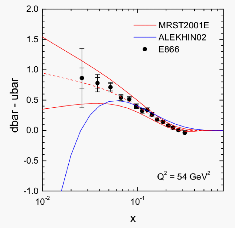
Since we analyze charged lepton–nucleon scattering the non–singlet structure functions require the distribution $x(\overline{d}-\overline{u})(x,Q^{2})$ as an input, which cannot easily be extracted in the DIS analysis, but can be determined from Drell–Yan data [39]. We refer to a parameterization in [40] at $Q^{2}=1\,\mbox{GeV}^{2}$ which has been evolved to $Q_{0}^{2}=4\,\mbox{GeV}^{2}$. An illustration is given in Figure 1, containing also the older parton parameterization [12] which has been updated recently [13].

Part of the data is situated at low values of $Q^{2}$ and large values of $x$ which have to be corrected for target mass effects, cf. [41]. The respective numerical effects are discussed below, see Figures 5, 6 and 8.

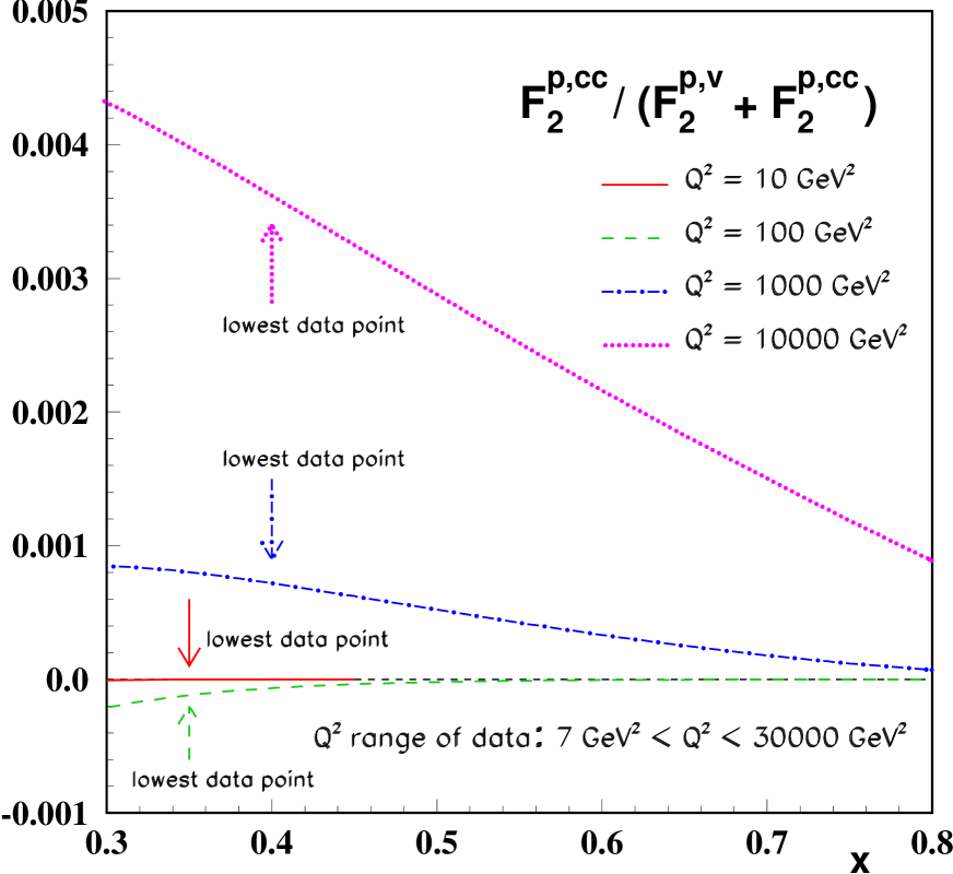
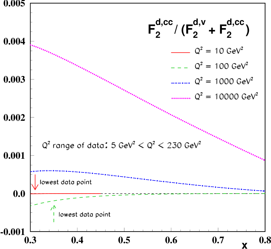
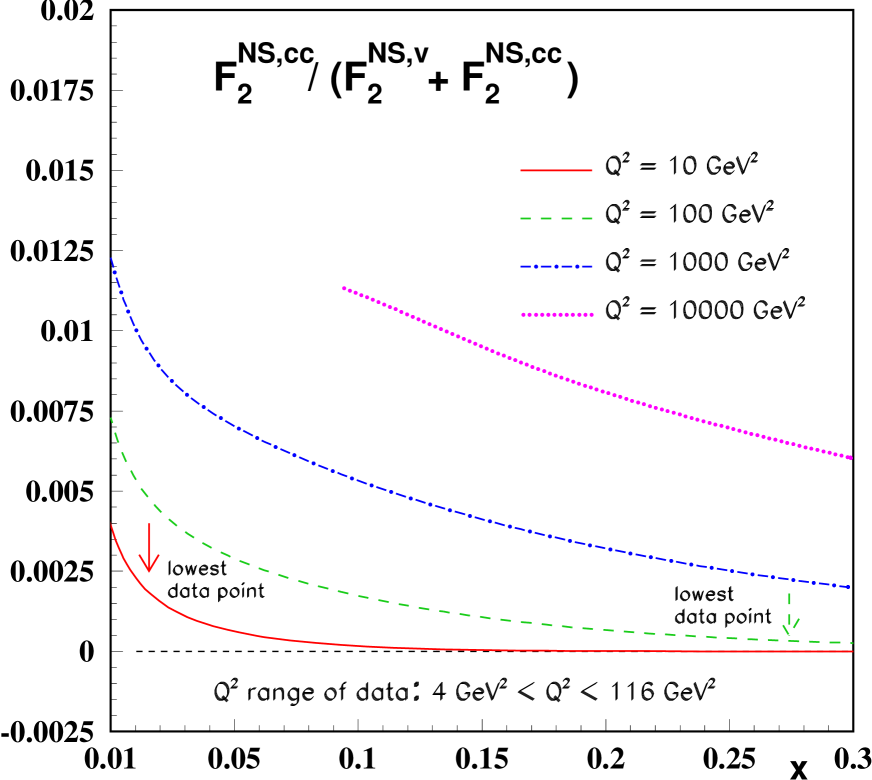
Beginning with $O(\alpha_{s}^{2})$ the non–singlet structure functions receive heavy flavor contributions due to the Compton–process $\gamma^{*}+q(\overline{q})\rightarrow q(\overline{q})+g^{*}\rightarrow Q\overline{Q}$ and $\gamma^{*}+g^{*}\rightarrow Q\overline{Q}$, where the off–shell gluon is emitted from a light quark or anti–quark line in lowest order, [42]. As the present analysis is carried out in Mellin space one needs accurate and fast representations for the heavy flavor contributions, which were derived in Ref. [43] for all available heavy flavor Wilson coefficients. We accounted for these contributions in the present analysis. The numerical effects of these contributions for the case of $c\overline{c}$ production are shown in Figures 2, 3 and 4 for the proton and deuteron valence regions $x\geq 0.3$ and for $F_{2}^{\rm NS}(x,Q^{2})$ at $x\leq 0.3$ for a wide region in $Q^{2}$. The respective arrows mark the lowest data point in the analysis. Except of the very high $Q^{2}$ region, $Q^{2}\simeq 10000\,\mbox{GeV}^{2}$, where the relative contribution amounts to $O(0.4\%)$ the typical corrections are (far) below 1 per mille and are therefore widely negligible. The present analysis would require the $O(\alpha_{s}^{3})$ heavy flavor corrections for $F_{2}^{\rm NS}(x,Q^{2})$ as well, which were not yet calculated. From the $O(\alpha_{s}^{2})$ results we do not expect large additional effects in the non–singlet case, however. The $b\overline{b}$–contributions are even smaller.

Universal small-$x$ contribution to the evolution kernel for deep–inelastic scattering were derived in [46] in leading order. Resumming these effects with renormalization group techniques yields contributions on the level of 1–2% and less depending on the size of the subleading terms [47], which are important. Like in the flavor singlet case [48] the sub-, subsub-leading contributions, etc. turn out to be of quite similar size, however, with alternating sign, as the respective next term. This is easily verified expanding the available fixed oder results in consecutive powers in Mellin $1/N^{k}$, cf. also [7]. Hence, these effects do not affect the present analysis.

5 Fit Results

The flavor non–singlet analysis relies on the three complementary data sets: the structure functions $F_{2}^{p,d}(x,Q^{2})$ in the valence–quark region $x\geq 0.3$ and the combination of these structure functions $F_{2}^{\rm NS}(x,Q^{2})=2[F_{2}^{p}(x,Q^{2})-F_{2}^{d}(x,Q^{2})]$ . To isolate the twist–2 contributions to the deep–inelastic structure functions $F_{2}^{p,d}(x,Q^{2})$ cut–studies in $Q^{2}$ and $W^{2}$ were performed. It turns out, that power corrections are widely absent in the kinematic region $Q^{2}\geq 4\,\mbox{GeV}^{2},W^{2}>12.5\,\mbox{GeV}^{2}$ . We therefore choose these cuts for the whole data set to perform a twist–2 non–singlet QCD analysis. We further unfold the target mass corrections [41] for all data.

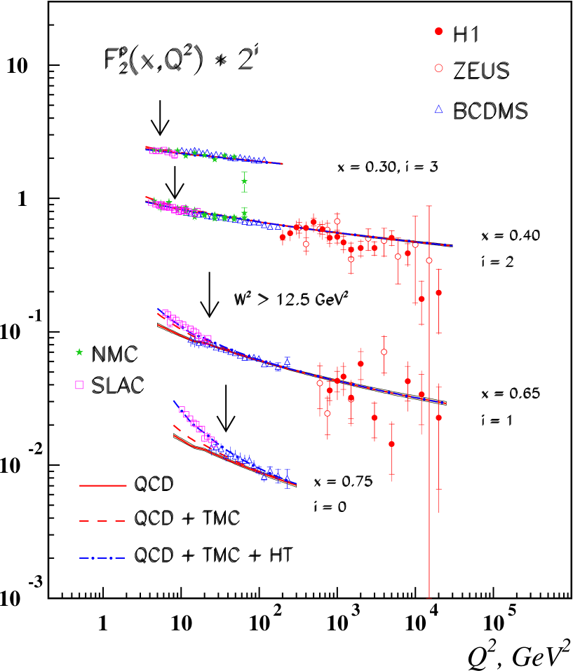
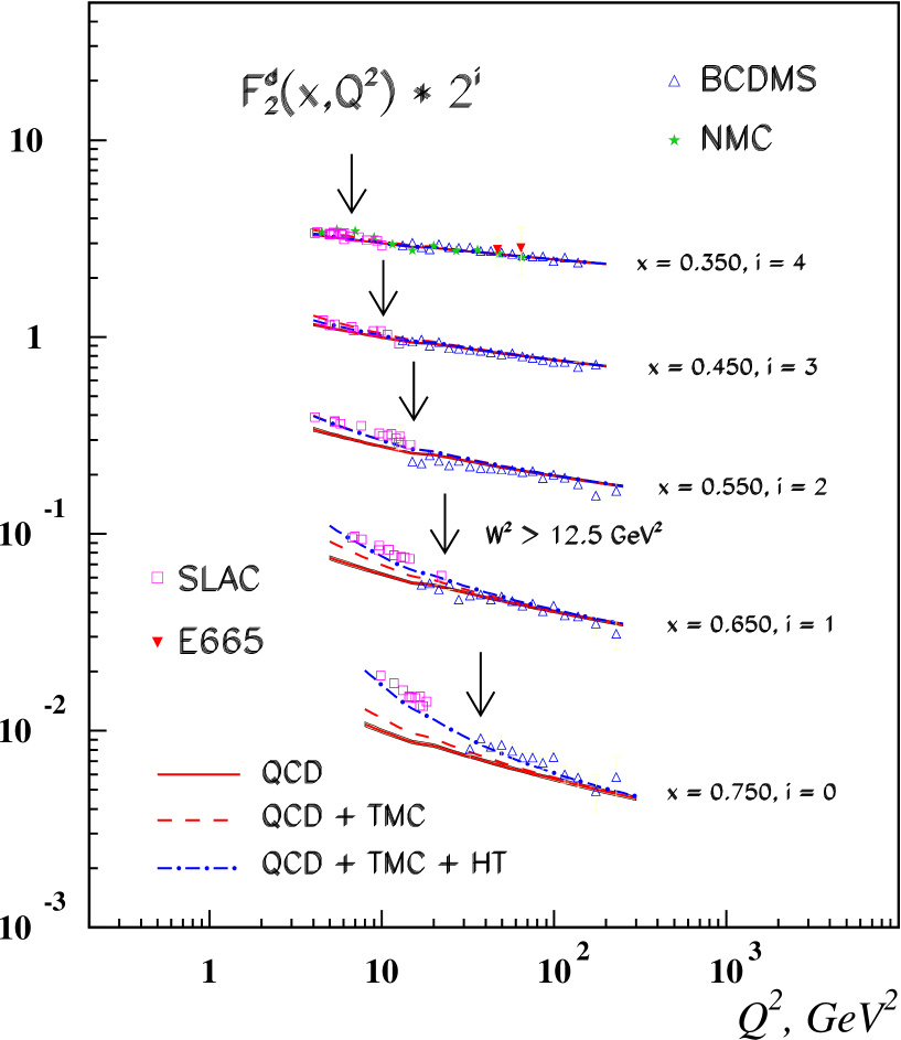
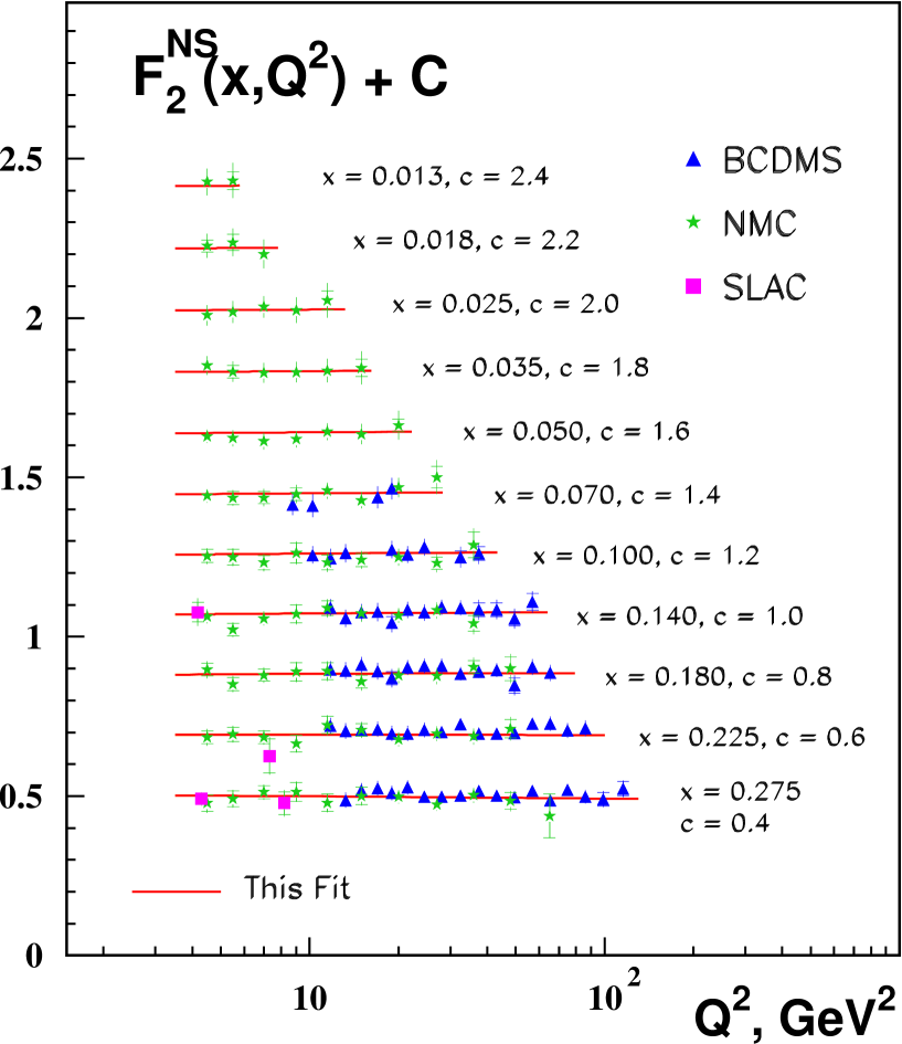
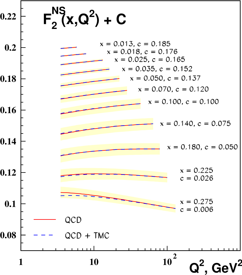
In Figure 5 the proton data for $F_{2}(x,Q^{2})$ are shown in the valence quark region $x\geq 0.3$ indicating the above cuts by an arrow. The solid lines correspond to the NNLO QCD fit and the dashed lines correspond to the NNLO QCD fit adding target mass corrections. We extrapolate these fits to the region $12.5\,\mbox{GeV}^{2}\geq W^{2}\geq 4\,\mbox{GeV}^{2}$. There, at higher values of $x$ a clear gap between the data and the QCD fit is seen. Figure 6 shows the corresponding results for the deuteron data. In the kinematic region $x\leq 0.3$ the above $W^{2}$ cut is ineffective. Figure 7 shows the result of the NNLO fit for this region. The effect of target mass corrections in the latter kinematic domain is shown in Figure 8, which turns out to be rather small.

In Table 2 we summarize the fit results for the parameters of the parton densities $xu_{v}(x,Q^{2}_{0})$, $xd_{v}(x,Q^{2}_{0})$ and $\Lambda_{\rm QCD}^{\rm N_{f}=4}$ in the $\overline{\rm MS}$–scheme in NLO, NNLO, and N³LO. The value of $\chi^{2}/ndf$ at the minimum improves from 0.89 at NLO to 0.84 at N³LO. In all the fits the covariance matrix is positive definite. As an example we show the covariance matrix of the NNLO fit in Table 3.

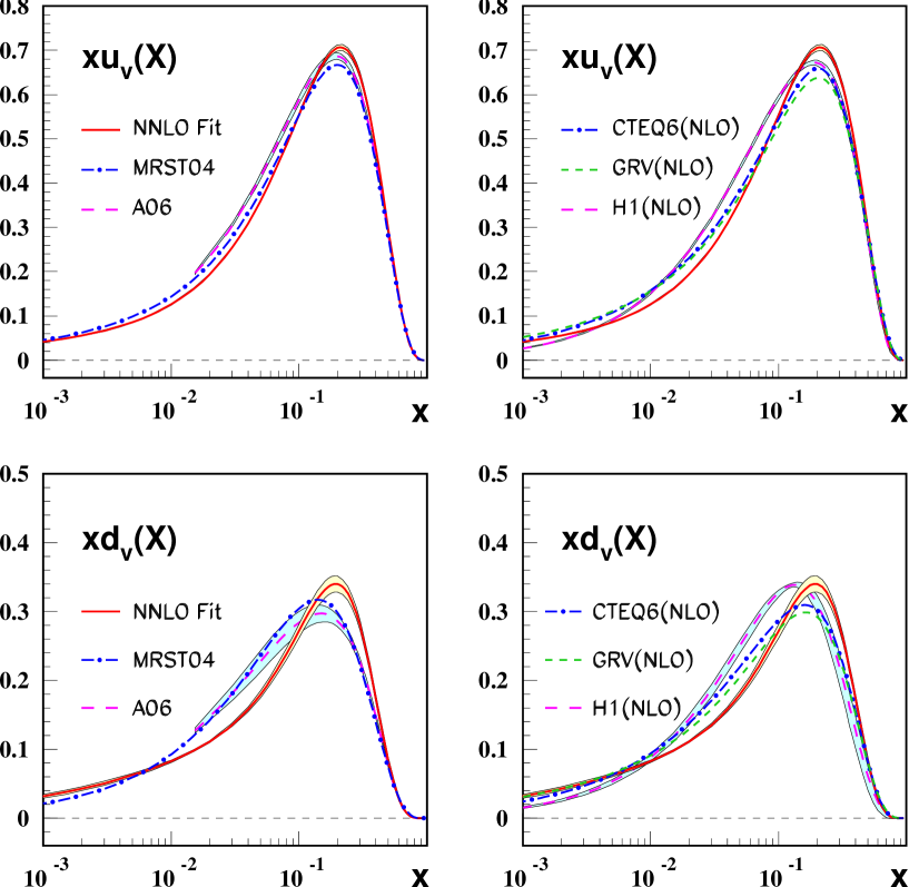
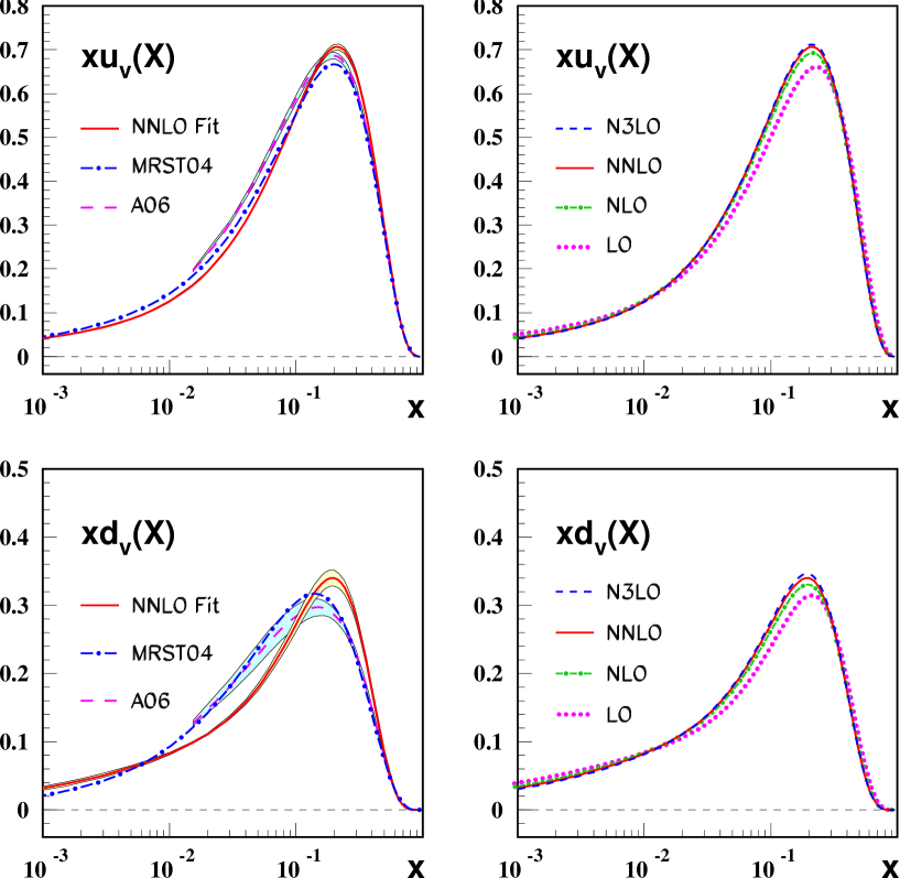
Figure 9 illustrates our fit results for $xu_{v}(x,Q^{2}_{0})$, $xd_{v}(x,Q^{2}_{0})$ at $Q_{0}^{2}=4\,\mbox{GeV}^{2}$ at NNLO with correlated errors (left figures). We compare to the results of [49] and a very recent analysis [13]. While there is very good agreement in the case of $xu_{v}(x,Q^{2}_{0})$ some differences at the $1\sigma$ level are visible for $xd_{v}(x,Q^{2}_{0})$. We also compare our results to some NLO analyses [19, 5, 50] (right figures). The spread here turns out to be somewhat larger than in the NNLO case. Note that the analyses we compare to are combined non-singlet/ singlet analyses and already different assumptions on the sea quark distributions may cause deviations for the non–singlet distributions in the range of smaller values of $x$.

In Figure 10 (right figures) we show the convergence of our analysis from LO to N³LO, which demonstrates perturbative stability for the parton distribution functions. The lines rise in the large $x$ region and drop slightly for low values of $x$. The shifts from NNLO to N³LO are far within the present error bands.

Another way to compare the NNLO fit results consists in forming moments of the distributions $u_{v}(x,Q^{2}),d_{v}(x,Q^{2}),$ and $u_{v}(x,Q^{2})-d_{v}(x,Q^{2})$. These moments may be directly compared with the results of lattice simulations at low pion masses using dynamical quarks in the near future. In Table 4 we present the lowest non–trivial moments of these distributions at $Q^{2}=Q_{0}^{2}$ in N³LO and NNLO and compare to the respective moments obtained for the parameterizations [49, 12, 13]. The recent parameterization [13] comes somewhat closer to our present parameterization then an earlier one [12] due to an improvement in the $x(\overline{d}(x,Q^{2})-\overline{u}(x,Q^{2}))$ distribution and taking into account off–shell effects in the target mass corrections [51]. The errors of the moments for [13] are slightly smaller than those in the present analysis. There are still some deviations, in particular for $d_{v}(x,Q^{2})$, but most of the values get very close.

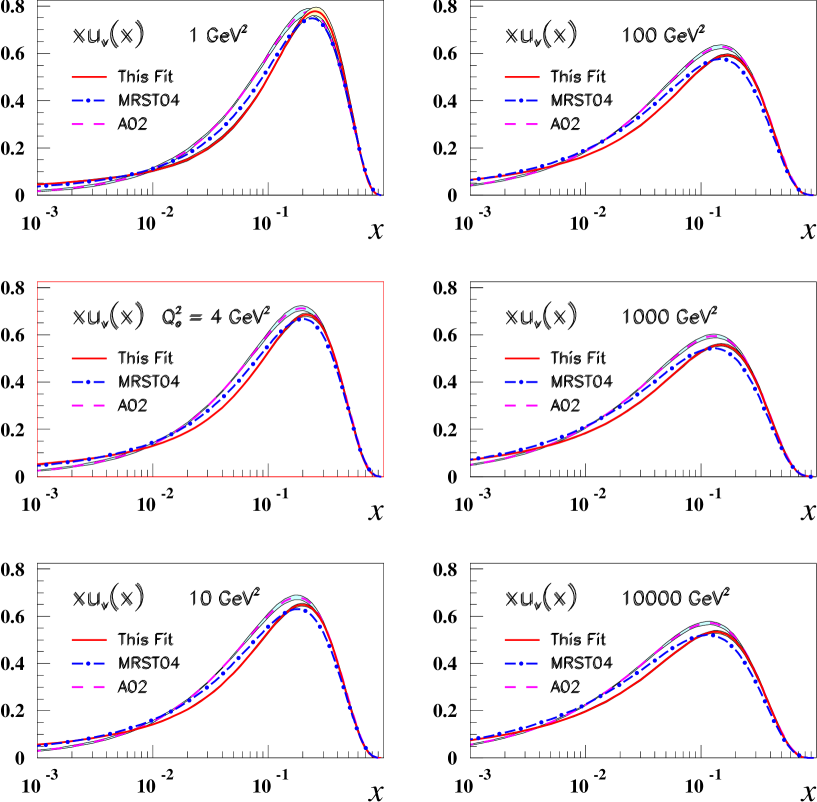
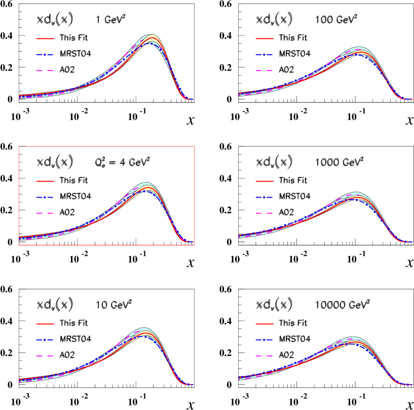
In Figures 11 and 12 we show the evolution of the valence quark densities $xu_{v}(x,Q^{2})$ and $xd_{v}(x,Q^{2})$ from $Q^{2}=1\,\mbox{GeV}^{2}$ to $Q^{2}=10^{4}\,\mbox{GeV}^{2}$ in the region $x~{}\epsilon~{}[10^{-3},1]$ at NNLO with correlated errors. To compute the respective error bands error propagation has to be performed through the evolution equations. We also compare to other NNLO analyses [49, 12]. With rising values of $Q^{2}$ the distributions flatten at large values of $x$ and rise at low values. Numerically fast parameterizations of the distributions $xu_{v}(x,Q^{2})$ and $xd_{v}(x,Q^{2})$ and their errors in the region $Q^{2}=[1,10^{6}]\,\mbox{GeV}^{2},~{}~{}x~{}\epsilon~{}[10^{-9},1]$ are performed and are available from the authors on request.

6 $\Lambda_{\rm QCD}$ and $\alpha_{s}(M_{Z}^{2})$

The QCD analysis is performed in NLO, NNLO and N³LO. The QCD scale $\Lambda_{\rm QCD}^{\rm N_{f}=4}$ is determined together with the parameters of the parton distributions with correlated errors. As an example the correlation matrix elements of the NNLO analysis are shown in Table 3.

In spite of the unknown 4–loop anomalous dimensions one may wonder whether any statement can be made on the non–singlet parton distributions and $\Lambda_{\rm QCD}$ at the 4–loop level. The 3–loop Wilson coefficients are known [8] and the question arises, which effect has the 4–loop anomalous dimension if compared to the Wilson coefficient. The gross behaviour of the 4–loop anomalous dimension may be Padé–approximated and we will allow a $\pm$ 100% error for it in the analysis. After the present analysis was finished, the 2nd moment of the 4–loop anomalous dimension was calculated in [10]

$$\gamma_{2} = \gamma_{2}^{(0)}a_{s}+\gamma_{2}^{(1)}a_{s}^{2}+\gamma_{2}^{(2)}a_{s}^{3}+\gamma_{2}^{(3)}a_{s}^{4}$$ (22)

$$= \frac{32}{9}a_{s}+\frac{9440}{243}a_{s}^{2}+\left[\frac{3936832}{6561}-\frac{10240}{81}\zeta_{3}\right]a_{s}^{3}$$

$$+\left[\frac{1680283336}{1777147}-\frac{24873952}{6561}\zeta_{3}+\frac{5120}{3}\zeta_{4}-\frac{56969}{243}\zeta_{5}\right]a_{s}^{4}$$

and can be compared to the Padé–approximant

$$\gamma_{n}^{\rm Pade} = \frac{{\gamma_{n}^{(2)}}^{2}}{\gamma_{n}^{(1)}}~{}.$$ (23)

For the second moment we found a deviation of about 20% only in the $O(a_{s}^{4})$ term, which is far inside our uncertainty margins in the non–singlet case. The variation in $\Lambda_{\rm QCD}$ varying the 4–loop anomalous dimension between zero and twice the value of the Padé–approximant amounts to $\pm 2\,\mbox{MeV}$. Thus $\Lambda_{\rm QCD}$ at $O(a_{s}^{4})$ accuracy is widely determined by the 3–loop Wilson coefficient and the behaviour of $a_{s}(Q^{2})$ to 4–loop order.

Table 5 summarizes our fit results comparing $\Lambda_{\rm QCD}^{\rm N_{f}=4}$ and $\alpha_{s}(M_{Z}^{2})$ for the NLO, NNLO and N³LO analysis. The NNLO value of $\Lambda_{\rm QCD}^{\rm N_{f}=4}$ is found to be smaller than the NLO value, while the N³LO value comes out somewhat higher than the NNLO value at about the same experimental error. The pattern of central values from NLO to N³LO shows the convergence of the analysis, which is illustrated by the decreasing difference of these values. This measure of convergence is more significant than varying the scales of the problem, which is less well defined since the range of variations is arbitrary.

We compare the results of the present analysis to results obtained in the literature at NLO and NNLO in Table 6. Most of the NLO values for $\alpha_{s}(M_{Z}^{2})$ shown were determined in combined singlet- and non–singlet analyses, partly including jet–data in $\overline{p}p$ scattering. Not in all analyses the correlation matrices for the parameters of the fit were presented. The NLO values for $\alpha_{s}(M_{Z}^{2})$ are larger than those at NNLO as several analyses, which performed both fits, show. The difference of both values, however, is not always the same, most likely due to the type of analysis being performed (singlet and non-singlet, non-singlet only, etc.), in which also partly different data sets are analyzed.

As outlined above we perform kinematic cuts in the present analysis to eliminate as widely as possible higher twist effects. In this way a significant part of the SLAC data is cut away due to the requirement of a minimal value $W^{2}=12.5\,\mbox{GeV}^{2}$. Other analyses, cf. [12, 18], fit phenomenological models for the higher twist contributions. In a precision determination of $\alpha_{s}(M_{Z}^{2})$ we do not follow this way since a thorough description of these contributions in terms of the light-cone expansion, including the description of the 4–, 6– etc. parton correlation functions, the corresponding Wilson coefficients and anomalous dimensions, is not known yet, but would be required.

A significant part of the data in the non–singlet case is due to the BCDMS measurements [2]. These data have repeatedly being criticized to deliver a too small value for $\Lambda_{\rm QCD}$, respectively $\alpha_{s}(M_{Z}^{2})$. Let us therefore revisit associated analyses. The NLO BCDMS–fit was confirmed in [52] both in the singlet and a separate non–singlet analysis with practically the same value for $\Lambda_{\rm QCD}^{\rm N_{f}=4,\overline{\rm MS}}$,

$$\Lambda_{\rm QCD}^{\rm N_{f}=4,\overline{\rm MS}}=198\pm 20\,\mbox{MeV}~{};~{}~{}\alpha_{s}(M_{Z}^{2})=0.1096\footnotesize{\begin{array}[]{c}+0.0016\\ -0.0018\end{array}}~{}.$$ (26)

In a re-analysis of the BCDMS data [53] using somewhat less severe $y$ cuts than applied in the present paper the corresponding value

$$\Lambda_{\rm QCD}^{\rm N_{f}=4,\overline{\rm MS}}=257\pm 40\,\mbox{MeV},$$ (27)

was found, which is numerically in accordance with our result. However, in [53] the flavor threshold matching in $\alpha_{s}(\mu^{2})$ was performed at the rather high scales $4m_{Q}^{2},~{}~{}m_{c}^{2}=9\,\mbox{GeV}^{2},m_{b}^{2}=80\,\mbox{GeV}^{2}$. Usually the convention is to match at $m_{c}$ and $m_{b}$. Therefore, the results of [53] cannot be compared to other analyses directly. We preformed the NLO analysis with these matching conditions and obtained

$$\Lambda_{\rm QCD}^{\rm N_{f}=4,\overline{\rm MS}}=254\pm 26\,\mbox{MeV};~{}~{}\alpha_{s}(M_{Z}^{2})=0.1127\footnotesize{\begin{array}[]{c}+0.0018\\ -0.0019\end{array}}$$ (30)

and do not confirm the rather high values of $\alpha_{s}(M_{Z}^{2})$ reported in [53].

Non–singlet QCD analyses were also performed for neutrino data. In [15] the CCFR iron data on $xF_{3}(x,Q^{2})$ [54] were analyzed in NLO and NNLO using fixed moments. Likewise a NNLO analysis was performed in [14]. Iron data suffer form the EMC effect, Fermi motion and other nuclear effects, as re-scattering, for which the QCD scaling violations are not known in detail. In [15] rather large values for $\Lambda_{\rm QCD}^{\rm N_{f}=4,\overline{\rm MS}}$

$$\Lambda_{\rm QCD,NLO}^{\rm N_{f}=4,\overline{\rm MS}}=371\pm 72\,\mbox{MeV}$$ (31)

$$\Lambda_{\rm QCD,NNLO}^{\rm N_{f}=4,\overline{\rm MS}}=316\pm 51\,\mbox{MeV}$$ (32)

are obtained, which are higher than the values obtained in the analyses based on $F_{2}^{p,d}(x,Q^{2})$ data, still showing the pattern that the NNLO value is lower than the NLO value. In a quite similar analysis in Ref. [14] on the other hand, values close to the results of the present analysis are obtained,

$$\Lambda_{\rm QCD,NLO}^{\rm N_{f}=4,\overline{\rm MS}} = 281\pm 57\,\mbox{MeV}$$ (33)

$$\Lambda_{\rm QCD,NNLO}^{\rm N_{f}=4,\overline{\rm MS}} = 255\pm 55\,\mbox{MeV}~{}.$$ (34)

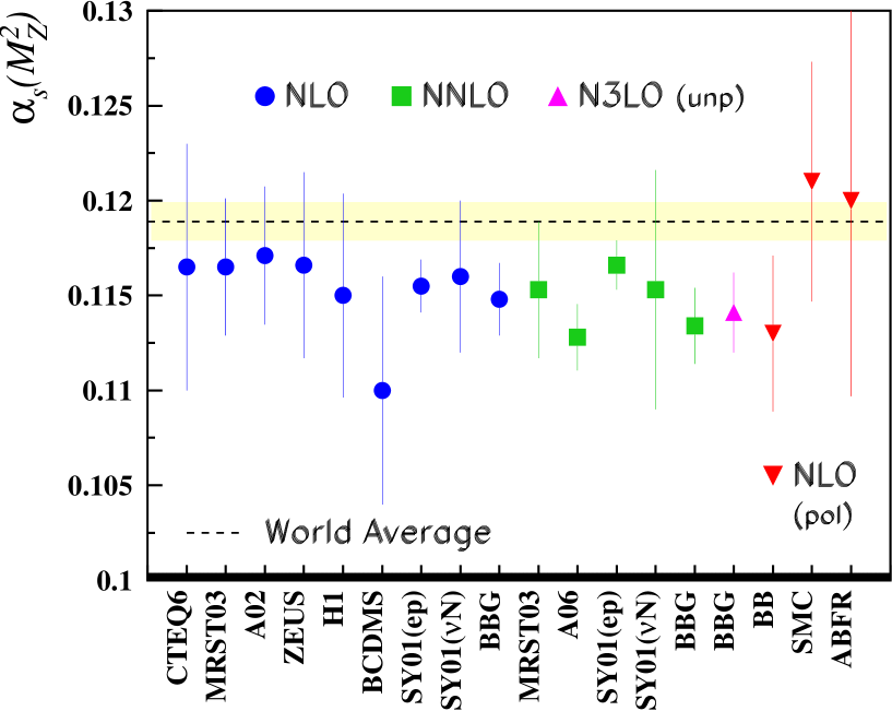
In Figure 13 we compare the results of different NLO and NNLO QCD unpolarized and polarized DIS analyses for $\alpha_{s}(M_{Z}^{2})$ with the results obtained in the present paper and the world average for $\alpha_{s}(M_{Z}^{2})$

$$\alpha_{s}(M_{Z}^{2})=0.1189\pm 0.0010~{},$$ (35)

which has been determined in [55] recently. In most of the cases the central values lay below the world average. Yet most of the NLO results are 1$\sigma$ compatible with the world average and an increasing number of NNLO results departs to lower values. In the case of polarized deep inelastic scattering at present only NLO analyses are performed with larger errors than in the unpolarized case, which is due the current experimental errors of the polarization asymmetries.

We finally would like to mention results on $\Lambda_{\rm QCD}^{\rm N_{f}=2,\overline{\rm MS}}$ from lattice calculations with two dynamical quark flavors [61, 62]

$$\Lambda_{\rm QCD}^{\rm N_{f}=2,\overline{\rm MS}} = 245\pm 16{\rm(stat.)}\pm 16{\rm(syst.)}\,\mbox{MeV}$$ (36)

$$\Lambda_{\rm QCD}^{\rm N_{f}=2,\overline{\rm MS}} = 261\pm 17{\rm(stat.)}\pm 26{\rm(syst.)}\,\mbox{MeV}~{}.$$ (37)

These values are very close to the $N_{f}=0$ lattice results with rather small errors. It will be interesting to see which values will be obtained for four dynamical quark flavors in the future.

7 Higher Twist

The cuts applied in $Q^{2}$ and $W^{2}$, $Q^{2}\geq 4\,\mbox{GeV}^{2}$ and $W^{2}\geq 12.5\,\mbox{GeV}^{2}$ in the standard analysis do widely eliminate higher twist effects from the data sample. Still the region for deep–inelastic scattering ranges to lower values of $W^{2}\geq 4\,\mbox{GeV}^{2}$ keeping the cut in $Q^{2}$. The data in the kinematic region

$$Q^{2}\geq 4\,\mbox{GeV}^{2},~{}~{}~{}~{}~{}~{}4\leq W^{2}\leq 12.5\,\mbox{GeV}^{2}$$ (38)

may thus be used to yield information on power corrections in $F_{2}^{p}(x,Q^{2})$ and $F_{2}^{d}(x,Q^{2})$. For this purpose we extrapolate the QCD fit results obtained for $W^{2}\geq 12.5\,\mbox{GeV}^{2}$ to the region (38) and form the difference between data and theory, applying target mass corrections in addition. The empirical higher twist coefficient

$$F_{2}^{\rm exp}(x,Q^{2})=O_{\rm TMC}[F_{2}^{\rm tw2}(x,Q^{2})]\cdot\left(1+\frac{C_{\rm HT}(x,Q^{2})}{Q^{2}[\,\mbox{GeV}^{2}]}\right)$$ (39)

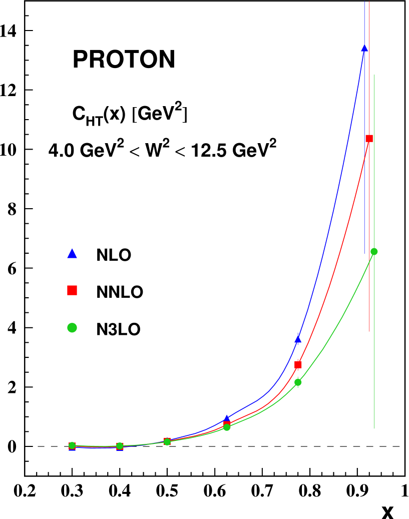
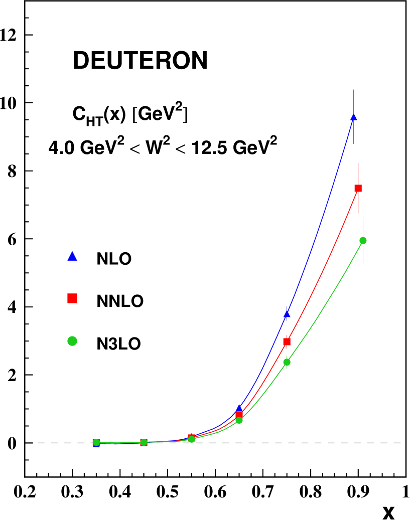
is extracted. Here the operation $O_{\rm TMC}[...]$ denotes taking the target mass corrections of the twist–2 contributions to the respective structure function. The coefficients $C_{\rm HT}(x,Q^{2})$ are determined in bins of $x$ and $Q^{2}$ and are then averaged over $Q^{2}$. The extracted distributions for $C_{\rm HT}(x)$ are depicted in Figures 14 and 15 for the non–singlet case considering scattering off the proton and the deuteron target, respectively. The coefficient $C_{\rm HT}(x)$ grows towards large $x$. We find a similar pattern if compared to the early NLO analysis [63]. Comparing the extractions for the case of calculating $F_{2}^{\rm tw2}(x,Q^{2})$ in NLO, NNLO and N³LO a gradual reduction of $C_{\rm HT}(x)$ is obtained, i.e. higher twist extractions describing the twist–2 contributions by low order in perturbation theory only lead to incorrect results. As seen from Figures 14, 15 $C_{\rm HT}(x)$ is widely independent of the target comparing the results for deeply inelastic scattering off protons and deuterons, after nuclear wave function corrections were performed. Beyond $x\simeq 0.9$ the errors for $C_{\rm HT}(x)$ become very large.

8 Conclusions

We performed a twist–2 QCD analysis of the non–singlet world data up to NNLO and N³LO and determined the valence quark densities $xu_{v}(x,Q^{2})$ and $xd_{v}(x,Q^{2})$ with correlated errors in the $\overline{\rm MS}$–scheme using conservative kinematic cuts for the data. Parameterizations of these parton distribution functions and their errors were derived in a wide range of $x$ and $Q^{2}$ as fit results at LO, NLO, NNLO, and N³LO. In the analysis the QCD scale $\Lambda_{\rm QCD}^{\rm N_{f}=4}$ and the strong coupling constant $\alpha_{s}(M_{Z}^{2})$, were determined up to N³LO. The effect of the 4–loop anomalous dimension, if compared to the 3–loop Wilson coefficient and the 4–loop effects in $\alpha_{s}(\mu^{2})$ turn out to be rather weak. The corresponding estimates, based on a Padé-approximation compare very well with the recently calculated second moment of the 4–loop anomalous dimension. The assumption of a $\pm 100\%$ error on the Padé-approximant results into a marginal shift of $\pm 2\,\mbox{MeV}$ in $\Lambda_{\rm QCD}^{\rm N_{f}=4}$ only. The convergence of the central values for $\Lambda_{\rm QCD}^{\rm N_{f}=4}$ and $\alpha_{s}(M_{Z}^{2})$ from NLO to N³LO shows the stability of the analysis and provides some measure of remaining higher order effects. Moments for the valence quark distributions with correlated errors at NNLO and N³LO were calculated for comparisons with upcoming lattice simulations. Higher twist effects both in $F_{2}^{p}$ and $F_{2}^{d}$ are extracted extrapolating the twist–2 results to the region $W^{2}\leq 12.5\,\mbox{GeV}^{2}$. These contributions are found to be widely target independent and decrease with rising order in the coupling constant for the twist–2 contributions.

Acknowledgment. This work was supported in part by DFG Sonderforschungsbereich Transregio 9, Computergestützte Theoretische Physik. We thank J. Stirling for the kind permission to show Figure 1 and for discussions. We would like to thank E. Reya and S. Alekhin for communicating their recent results to us. We would like to thank E. Christy, R. Ent, M. Glück, K. Jansen, C. Keppel, M. Klein, W. Melnitchouk, S. Moch, G. Schierholz, R. Sommer, A.W. Thomas and U. Wolff for discussions and DESY for support of this project.

9 Tables

Experiment	$x$	$Q^{2},~{}\,\mbox{GeV}^{2}$	$F_{2}^{p}$	$F_{2}^{p}~{}cuts$	$F_{2}^{p}~{}HT$	Norm
BCDMS (100)	0.35 – 0.75	11.75 – 75.00	51	21	10	1.005
BCDMS (120)	0.35 – 0.75	13.25 – 75.00	59	32	4	0.998
BCDMS (200)	0.35 – 0.75	32.50 – 137.50	50	28	0	0.998
BCDMS (280)	0.35 – 0.75	43.00 – 230.00	49	26	0	0.998
NMC (comb)	0.35 – 0.50	7.00 – 65.00	15	14	6	1.000
SLAC (comb)	0.30 – 0.62	7.30 – 21.39	57	57	259	1.013
H1 (hQ2)	0.40 – 0.65	200 – 30000	26	26	0	1.020
ZEUS (hQ2)	0.40 – 0.65	650 – 30000	15	15	0	1.007
$proton$			322	227	279
Experiment	$x$	$Q^{2},\,\mbox{GeV}^{2}$	$F_{2}^{d}$	$F_{2}^{d}~{}cuts$	$F_{2}^{d}~{}~{}HT$	Norm
BCDMS (120)	0.35 – 0.75	13.25 – 99.00	59	32	4	1.001
BCDMS (200)	0.35 – 0.75	32.50 – 137.50	50	28	0	0.998
BCDMS (280)	0.35 – 0.75	43.00 – 230.00	49	26	0	1.003
NMC (comb)	0.35 – 0.50	7.00 – 65.00	15	14	6	1.000
SLAC (comb)	0.30 – 0.62	10.00 – 21.40	59	59	268	0.990
$deuteron$			232	159	278
Experiment	$x$	$Q^{2},\,\mbox{GeV}^{2}$	$F_{2}^{NS}$	$F_{2}^{NS}~{}(cuts)$	$F_{2}^{NS}~{}~{}HT$	Norm
BCDMS (120)	0.070 – 0.275	8.75 – 43.00	36	30	0	0.983
BCDMS (200)	0.070 – 0.275	17.00 – 75.00	29	28	0	0.999
BCDMS (280)	0.100 – 0.275	32.50 – 115.50	27	26	0	0.997
NMC (comb)	0.013 – 0.275	4.50 – 65.00	88	53	0	1.000
SLAC (comb)	0.153 – 0.293	4.18 – 5.50	28	28	1	0.994
$non-singlet$			208	165	1
$total$			762	551	558

Table 1: Number of data points for the non–singlet QCD analysis with their $x$ and $Q^{2}$ ranges. In the first column are given (in parentheses) the beam momentum in GeV of the the respective data set (number), a flag whether the data come from a combined analysis of all beam momenta (comb) or whether the data are taken at high momentum transfer (hQ2). The fourth column ($F_{2}$) contains the number of data points according to the cuts: $Q^{2}>4~{}{\,\mbox{GeV}^{2}}$, $W^{2}>12.5~{}{\,\mbox{GeV}^{2}}$, $x>0.3$ for $F_{2}^{p}$ and $F_{2}^{d}$ and $x<0.3$ for $F_{2}^{NS}$. The reduction of the number of data points by the additional cuts on the BCDMS data ($y>0.3$) and on the NMC data ($Q^{2}>8~{}{\,\mbox{GeV}^{2}}$) are given in the 5th column ($F_{2}~{}cuts$). The 6th column ($F_{2}~{}HT$) contains the number of data points in the range $4~{}{\,\mbox{GeV}^{2}}<W^{2}<12.5~{}{\,\mbox{GeV}^{2}}$ used to fit the higher twist coefficients $C_{HT}(x)$ for the proton and deuteron data. In the last column the normalization shifts (see text) are listed.

		NLO	NNLO	N3LO
$u_{v}$	$a$	0.274 $\pm$ 0.027	0.291 $\pm$ 0.008	0.298 $\pm$ 0.008
	$b$	3.909 $\pm$ 0.040	4.013 $\pm$ 0.037	4.032 $\pm$ 0.037
	$\rho$	6.003	6.227	6.042
	$\gamma$	35.089	35.629	35.492
$d_{v}$	$a$	0.461 $\pm$ 0.030	0.488 $\pm$ 0.033	0.500 $\pm$ 0.034
	$b$	5.683 $\pm$ 0.228	5.878 $\pm$ 0.239	5.921 $\pm$ 0.243
	$\rho$	–3.699	–3.639	–3.618
	$\gamma$	16.491	16.445	16.414
$\Lambda_{\rm QCD}^{\rm N_{f}=4}$, MeV		265 $\pm$ 27	226 $\pm$ 25	234 $\pm$ 26
$\chi^{2}/ndf$		484/546 = 0.89	472/546 = 0.86	461/546 = 0.84

Table 2: Parameter values of the NLO, NNLO and N³LO non–singlet QCD fit at $Q_{0}^{2}=4~{}\,\mbox{GeV}^{2}$. The values without error have been fixed after a first minimization since the data do not constrain these parameters well enough (see text).

NNLO	$\Lambda_{\rm QCD}^{\rm N_{f}=4}$	$a_{u_{v}}$	$b_{u_{v}}$	$a_{d_{v}}$	$b_{d_{v}}$
$\Lambda_{QCD}^{(4)}$	6.45E-4
$a_{u_{v}}$	9.03E-5	5.75E-5
$b_{u_{v}}$	-3.37E-4	1.55E-4	1.40E-3
$a_{d_{v}}$	1.92E-4	-8.97E-6	-4.69E-4	1.07E-3
$b_{d_{v}}$	9.19E-4	5.82E-5	-3.30E-3	7.21E-3	5.72E-2

Table 3: The covariance matrix of the NNLO non–singlet QCD fit at $Q_{0}^{2}=4~{}\,\mbox{GeV}^{2}$.

$f$	$n$	N3LO	NNLO	MRST04	A02	A06
$u_{v}$	2	0.3006 $\pm$ 0.0031	0.2986 $\pm$ 0.0029	0.285	0.304	0.2947
	3	0.0877 $\pm$ 0.0012	0.0871 $\pm$ 0.0011	0.082	0.087	0.0843
	4	0.0335 $\pm$ 0.0006	0.0333 $\pm$ 0.0005	0.032	0.033	0.0319
$d_{v}$	2	0.1252 $\pm$ 0.0027	0.1239 $\pm$ 0.0026	0.115	0.120	0.1129
	3	0.0318 $\pm$ 0.0009	0.0315 $\pm$ 0.0008	0.028	0.028	0.0275
	4	0.0106 $\pm$ 0.0004	0.0105 $\pm$ 0.0004	0.009	0.010	0.0092
$u_{v}-d_{v}$	2	0.1754 $\pm$ 0.0041	0.1747 $\pm$ 0.0039	0.171	0.184	0.182
	3	0.0559 $\pm$ 0.0015	0.0556 $\pm$ 0.0014	0.055	0.059	0.057
	4	0.0229 $\pm$ 0.0007	0.0228 $\pm$ 0.0007	0.022	0.024	0.023

Table 4: Comparison of low order moments at $Q_{0}^{2}=4~{}\,\mbox{GeV}^{2}$ from our non–singlet N³LO and NNLO QCD analyses with the NNLO analyses MRST04 [49], A02 [12] and A06 [13] derived from global analyses, resp. combined singlet/non-singlet fits.

	$\Lambda_{\rm QCD}^{\rm N_{f}=4}$, MeV	$\alpha_{s}(M_{Z}^{2})$
NLO	265 $\pm$ 27	0.1148 $\begin{array}[]{c}+0.0019\\ -0.0019\end{array}$ (expt)
NNLO	226 $\pm$ 25	0.1134 $\begin{array}[]{c}+0.0019\\ -0.0021\end{array}$ (expt)
N3LO	234 $\pm$ 26	0.1141 $\begin{array}[]{c}+0.0020\\ -0.0022\end{array}$ (expt)

Table 5: $\Lambda_{\rm QCD}^{\rm N_{f}=4}$ and $\alpha_{s}(M_{Z}^{2})$ at NLO, NNLO and N³LO.

	$\alpha_{s}(M_{Z}^{2})$	expt	theory	model	Ref.
NLO
CTEQ6	0.1165	$\pm$0.0065			[19]
MRST03	0.1165	$\pm$0.0020	$\pm$0.0030		[11]
A02	0.1171	$\pm$0.0015	$\pm$0.0033		[12]
ZEUS	0.1166	$\pm$0.0049		$\pm$0.0018	[56]
H1	0.1150	$\pm$0.0017	$\pm$0.0050	$\begin{array}[]{c}+0.0009\\ -0.0005\end{array}$	[5]
BCDMS	0.110	$\pm$0.006			[2]
GRS	0.112				[18]
BBG	0.1148	$\pm$ 0.0019
BB (pol)	0.113	$\pm$0.004	$\begin{array}[]{c}+0.009\\ -0.006\end{array}$		[58]
NNLO
MRST03	0.1153	$\pm$0.0020	$\pm$0.0030		[11]
A02	0.1143	$\pm$0.0014	$\pm$0.0009		[12]
SY01(ep)	0.1166	$\pm$0.0013			[14]
SY01($\nu$N)	0.1153	$\pm$0.0063			[14]
GRS	0.111				[18]
A06	0.1128	$\pm$ 0.0015			[13]
BBG	0.1134	$\begin{array}[]{c}+0.0019\\ -0.0021\end{array}$
N3LO
BBG	0.1141	$\begin{array}[]{c}+0.0020\\ -0.0022\end{array}$

Table 6: Comparison of $\alpha_{s}(M_{Z}^{2})$ values from NLO, NNLO, and N³LO QCD analyses.

10 Figures

Figure 1: The MRST parameterization of $(\bar{d}-\bar{u})$ [40] describing the E866 data [39]. Here also compared with a parameterization given in [12].[Courtesy by J. Stirling.]

Figure 2: Relative size of the NLO contribution due to $c\overline{c}$–production for $m_{c}=1.5\,\mbox{GeV}$ for $F_{2}^{p}(x,Q^{2})$ in the valence quark region.

Figure 3: Relative size of the NLO contribution due to $c\overline{c}$–production for $m_{c}=1.5\,\mbox{GeV}$ for $F_{2}^{d}(x,Q^{2})$ in the valence quark region.

Figure 4: Relative size of the NLO contribution due to $c\overline{c}$–production for $m_{c}=1.5\,\mbox{GeV}$ for $F_{2}^{\rm NS}(x,Q^{2})=2[F_{2}^{p}(x,Q^{2})-F_{2}^{d}(x,Q^{2})]$ in the region $0.01\leq x\leq 0.3$.

Figure 5: The structure function $F_{2}^{p}$ as function of $Q^{2}$ in intervals of $x$. Shown are the pure QCD fit in NNLO (solid line) and the contributions from target mass corrections TMC (dashed line) and higher twist HT (dashed–dotted line). The arrows indicate the regions with $W^{2}>12.5~{}{\,\mbox{GeV}^{2}}$. The shaded areas represent the fully correlated $1\sigma$ statistical error bands.

Figure 6: The structure function $F_{2}^{d}$ as function of $Q^{2}$ in intervals of $x$. Shown are the pure QCD fit in NNLO (solid line) and the contributions from target mass corrections TMC (dashed line) and higher twist HT (dashed–dotted line). The arrows indicate the regions with $W^{2}>12.5~{}{\,\mbox{GeV}^{2}}$. The shaded areas represent the fully correlated $1\sigma$ statistical error bands.

Figure 7: The structure function $F_{2}^{\rm NS}$ as function of $Q^{2}$ in intervals of $x$. Shown is the pure QCD fit in NNLO (solid lines) with its fully correlated $1\sigma$ statistical error band (shaded areas).

Figure 8: The structure function $F_{2}^{\rm NS}$ as function of $Q^{2}$ in intervals of $x$ without data points. Shown are the pure QCD fit in NNLO (solid lines) with its fully correlated $1\sigma$ statistical error band (shaded areas) and the contribution from target mass corrections TMC (dashed line).

Figure 9: The parton densities $xu_{v}$ and $xd_{v}$ at the input scale $Q_{0}^{2}=4.0~{}{\rm{\,\mbox{GeV}^{2}}}$ (solid line) compared to results obtained from NNLO analyses by MRST (dashed–dotted line) [49] and A06 (dashed line) [13] (left panels) and from NLO analyses by CTEQ6 (dashed–dotted line) [19], GRV (dashed line) [50] and H1 (long dashed line) [5] (right panels). The shaded areas represent the fully correlated $1\sigma$ statistical error bands.

Figure 10: Left panels: The parton densities $xu_{v}$ and $xd_{v}$ at the input scale $Q_{0}^{2}=4.0~{}\,\mbox{GeV}^{2}$ (solid line) compared to results obtained from NNLO analyses by MRST (dashed–dotted line) [49] and A06 (dashed line) [13]. The shaded areas represent the fully correlated $1\sigma$ statistical error bands. Right panels: Comparison of the same parton densities at different orders in QCD as resulting from the present analysis.

Figure 11: The parton density $xu_{v}$ at NNLO evolved up to $Q^{2}=10,000~{}{\,\mbox{GeV}^{2}}$ (solid lines) compared to results obtained by MRST (dashed–dotted line) [49] and A02 (dashed line) [12]. The shaded areas represent the fully correlated $1\sigma$ statistical error bands.

Figure 12: The parton density $xd_{v}$ at NNLO evolved up to $Q^{2}=10,000~{}{\,\mbox{GeV}^{2}}$ (solid lines) compared to results obtained by MRST (dashed–dotted line) [49] and A02 (dashed line) [12]. The shaded areas represent the fully correlated $1\sigma$ statistical error bands.

Figure 13: Comparison of different NLO, NNLO and N³LO measurements of the strong coupling constant $\alpha_{s}(M_{Z}^{2})$ in unpolarized and polarized deeply inealstic scattering. CTEQ6 [19], MRST03 [11], A02 [12], ZEUS [56], H1 [5], BCDMS [2], BBG: present analysis, SY01 [14], A06 [13], BB [58], SMC [59], ABFR [60].

Figure 14: The higher twist coefficient $C_{HT}(x)$ for the proton data as function of $x$ treating the twist–2 contributions in NLO, NNLO and N³LO.

Figure 15: The higher twist coefficient $C_{HT}(x)$ for the deuteron data as function of $x$ treating the twist–2 contributions in NLO, NNLO and N³LO.

References

-
[1]
K.G. Wilson, Phys. Rev. 179 (1969) 1699;
R.A. Brandt and G. Preparata, Fortschr. Phys. 18 (1970) 249;
W. Zimmermann, Lect. on Elementary Particle Physics and Quantum Field Theory, Brandeis Summer Inst., Vol. 1, (MIT Press, Cambridge, 1970), p. 395;
Y. Frishman, Ann. Phys. 66 (1971) 373. -
[2]
A.C. Benvenuti et al. [BCDMS Collaboration],
Phys. Lett. B 237 (1990) 592;
A.C. Benvenuti et al. [BCDMS Collaboration], Phys. Lett. B223 (1989) 485; Phys. Lett. B237 (1990) 592.
A.C. Benvenuti et al. [BCDMS Collaboration], Phys. Lett. B 237 (1990) 599. - [3] L. W. Whitlow, E. M. Riordan, S. Dasu, S. Rock and A. Bodek, Phys. Lett. B 282 (1992).
- [4] M. Arneodo et al. [New Muon Collaboration], Nucl. Phys. B 483 (1997) 3 [arXiv:hep-ph/9610231].
[5]
C. Adloff et al. [H1 Collaboration],
Eur. Phys. J. C 21 (2001) 33
[arXiv:hep-ex/0012053];
C. Adloff et al. [H1 Collaboration], Eur. Phys. J. C 30 (2003) 1 [arXiv:hep-ex/0304003]. -
[6]
J. Breitweg et al. [ZEUS Collaboration],
Eur. Phys. J. C 7 (1999) 609
[arXiv:hep-ex/9809005];
S. Chekanov et al. [ZEUS Collaboration], Eur. Phys. J. C 21 (2001) 443 [arXiv:hep-ex/0105090]. - [7] S. Moch, J. A. M. Vermaseren and A. Vogt, Nucl. Phys. B 688 (2004) 101 [arXiv:hep-ph/0403192].
- [8] J. A. M. Vermaseren, A. Vogt and S. Moch, Nucl. Phys. B 724 (2005) 3 [arXiv:hep-ph/0504242].
[9]
S. A. Larin, T. van Ritbergen and J. A. M. Vermaseren,
Nucl. Phys. B 427 (1994) 41;
S. A. Larin, P. Nogueira, T. van Ritbergen and J. A. M. Vermaseren, Nucl. Phys. B 492 (1997) 338 [arXiv:hep-ph/9605317];
A. Retey and J. A. M. Vermaseren, Nucl. Phys. B 604 (2001) 281 [arXiv:hep-ph/0007294];
J. Blümlein and J. A. M. Vermaseren, Phys. Lett. B 606 (2005) 130 [arXiv:hep-ph/0411111]. - [10] P.A. Baikov and K.G. Chetyrkin, in: Proceeedings of Loops and Legs in Quantum Field Theory, 2006, Eisenach, April, 2006, Nucl. Phys. B (Proc. Suppl.) to appear.
- [11] A. D. Martin, R. G. Roberts, W. J. Stirling and R. S. Thorne, arXiv:hep-ph/0307262.
- [12] S. Alekhin, Phys. Rev. D 68 (2003) 014002 [arXiv:hep-ph/0211096].
- [13] S. Alekhin, K. Melnikov and F. Petriello, arXiv:hep-ph/0606237 and private communication.
- [14] J. Santiago and F. J. Yndurain, Nucl. Phys. B 611 (2001) 447 [arXiv:hep-ph/0102247].
[15]
A. L. Kataev, G. Parente and A. V. Sidorov,
Nucl. Phys. Proc. Suppl. 116 (2003) 105
[arXiv:hep-ph/0211151];
A. L. Kataev, G. Parente and A. V. Sidorov, Phys. Part. Nucl. 34 (2003) 20 [Fiz. Elem. Chast. Atom. Yadra 34 (2003) 43] [arXiv:hep-ph/0106221]. - [16] J. Santiago and F. J. Yndurain, Nucl. Phys. B 563 (1999) 45 [arXiv:hep-ph/9904344].
- [17] J. Blümlein, H. Böttcher and A. Guffanti, Nucl. Phys. Proc. Suppl. 135 (2004) 152 [arXiv:hep-ph/0407089]; arXiv:hep-ph/0606309.
- [18] M. Glück, E. Reya and C. Schuck, arXiv:hep-ph/0604116.
- [19] J. Pumplin, D. R. Stump, J. Huston, H. L. Lai, P. Nadolsky and W. K. Tung, JHEP 0207 (2002) 012 [arXiv:hep-ph/0201195].
- [20] J. Pumplin, A. Belyaev, J. Huston, D. Stump and W. K. Tung, JHEP 0602 (2006) 032 [arXiv:hep-ph/0512167].
- [21] W. Furmanski and R. Petronzio, Z. Phys. C 11 (1982) 293.
[22]
W. L. van Neerven and E. B. Zijlstra,
Phys. Lett. B 272 (1991) 127;
E. B. Zijlstra and W. L. van Neerven, Nucl. Phys. B 383 (1992) 525. - [23] W. L. van Neerven and A. Vogt, Nucl. Phys. B 568 (2000) 263 [arXiv:hep-ph/9907472].
- [24] J. Blümlein and S. Kurth, Phys. Rev. D 60 (1999) 014018 [arXiv:hep-ph/9810241].
- [25] J. Blümlein, Comput. Phys. Commun. 133 (2000) 76 [arXiv:hep-ph/0003100].
- [26] J. Blümlein, Nucl. Phys. Proc. Suppl. 135 (2004) 225 [arXiv:hep-ph/0407044].
- [27] J. Blümlein and S. Moch, to appear.
- [28] J. Blümlein and S. O. Moch, Phys. Lett. B 614 (2005) 53 [arXiv:hep-ph/0503188].
- [29] J. Blümlein and V. Ravindran, Nucl. Phys. B 716 (2005) 128 [arXiv:hep-ph/0501178].
- [30] J. Blümlein and V. Ravindran, Nucl. Phys. B 749 (2006) 1 [arXiv:hep-ph/0604019].
- [31] K. G. Chetyrkin, B. A. Kniehl and M. Steinhauser, Phys. Rev. Lett. 79 (1997) 2184 [arXiv:hep-ph/9706430]. [32]
- [32] S. Bethke, J. Phys. G 26 (2000) R27 [arXiv:hep-ex/0004021].
- [33] W. A. Bardeen, A. J. Buras, D. W. Duke and T. Muta, Phys. Rev. D 18 (1978) 3998.
- [34] K. Abe et al. [E143 Collaboration], Phys. Lett. B 452 (1999) 194 [arXiv:hep-ex/9808028].
- [35] W. Melnitchouk and A. W. Thomas, Phys. Rev. C 52 (1995) 3373 [arXiv:hep-ph/9508311].
- [36] J. Blümlein and M. Klein, Nuclear Instruments and Methods in Physics Research, (NIM), A329 (1993) 112.
[37]
C.Pascaud and E.Zomer, preprint LAL-95-05;
M. Botje, Eur. Phys. J. C 14 (2000) 285 [arXiv:hep-ph/9912439]; M. Botje, J. Phys. G 28 (2002) 779 [arXiv:hep-ph/0110123;
D. Stump et al., Phys. Rev. D 65 (2002) 014012 [arXiv:hep-ph/0101051];
J. Pumplin et al., Phys. Rev. D 65 (2002) 014013 [arXiv:hep-ph/0101032];
A. D. Martin, R. G. Roberts, W. J. Stirling and R. S. Thorne, Eur. Phys. J. C 35 (2004) 325; [arXiv:hep-ph/0308087].
A. D. Martin, R. G. Roberts, W. J. Stirling and R. S. Thorne, Eur. Phys. J. C 28 (2003) 455 [arXiv:hep-ph/0211080]. - [38] F. James, CERN Program Library, Long Writeup D506 (MINUIT).
- [39] R. S. Towell et al. [FNAL E866/NuSea Collaboration], Phys. Rev. D 64 (2001) 052002 [arXiv:hep-ex/0103030].
- [40] A. D. Martin, R. G. Roberts, W. J. Stirling and R. S. Thorne, Eur. Phys. J. C 23 (2002) 73 [arXiv:hep-ph/0110215].
- [41] H. Georgi and H. D. Politzer, Phys. Rev. D 14 (1976) 1829.
[42]
E. Laenen, S. Riemersma, J. Smith, and W.L. van Neerven, Nucl. Phys. B392 (1993) 162, 229;
S. Riemersma, J. Smith, and W.L. van Neerven, Phys. Lett. B347 (1995) 143;
M. Buza, Y. Matiounine, J. Smith, R.L. Migneron and W.L. van Neerven, Nucl. Phys. B472 (1996) 611. - [43] S. I. Alekhin and J. Blümlein, Phys. Lett. B 594 (2004) 299 [arXiv:hep-ph/0404034].
- [44] J. Blümlein, A. De Freitas, S. Klein, S. Moch and W.L. van Neerven, to appear.
- [45] J. Blumlein, Nucl. Phys. Proc. Suppl. 157 (2006) 2.
- [46] R. Kirschner and L. N. Lipatov, Nucl. Phys. B 213 (1983) 122.
- [47] J. Blümlein and A. Vogt, Phys. Lett. B 370 (1996) 149 [arXiv:hep-ph/9510410]; Acta Phys. Polon. B 27 (1996) 1309 [arXiv:hep-ph/9603450].
[48]
J. Blümlein and A. Vogt,
Phys. Rev. D 58 (1998) 014020
[arXiv:hep-ph/9712546];
J. Blümlein, S. Riemersma and A. Vogt, Nucl. Phys. Proc. Suppl. 51C (1996) 30 [arXiv:hep-ph/9608470];
J. Blümlein, V. Ravindran, W. L. van Neerven and A. Vogt, arXiv:hep-ph/9806368. R. D. Ball and S. Forte, arXiv:hep-ph/9805315;
J. Blümlein, arXiv:hep-ph/9909449. - [49] A. D. Martin, R. G. Roberts, W. J. Stirling and R. S. Thorne, Phys. Lett. B 604 (2004) 61 [arXiv:hep-ph/0410230].
- [50] M. Glück, E. Reya and A. Vogt, Eur. Phys. J. C 5 (1998) 461 [arXiv:hep-ph/9806404].
- [51] S. Alekhin, private communication.
- [52] V.G Krivokhizhin et al., Z. Phys. C48 (1990) 347.
- [53] V.G Krivokhizhin and A.V. Kotikov, Physics of Atomic Nuclei, 11 (2005) 1935.
- [54] W. G. Seligman et al., Phys. Rev. Lett. 79 (1997) 1213.
- [55] S. Bethke, arXiv:hep-ex/0606035.
- [56] S. Chekanov et al. [ZEUS Collaboration], Phys. Rev. D 67 (2003) 012007 [arXiv:hep-ex/0208023].
- [57] R. S. Thorne, A. D. Martin and W. J. Stirling, arXiv:hep-ph/0606244.
- [58] J. Blümlein and H. Böttcher, Nucl. Phys. B 636 (2002) 225 [arXiv:hep-ph/0203155].
- [59] B. Adeva et al. [Spin Muon Collaboration], Phys. Rev. D 58 (1998) 112002.
- [60] G. Altarelli, R. D. Ball, S. Forte and G. Ridolfi, Nucl. Phys. B 496 (1997) 337 [arXiv:hep-ph/9701289].
- [61] M. Della Morte, R. Frezzotti, J. Heitger, J. Rolf, R. Sommer and U. Wolff [ALPHA Collaboration], flavours,” Nucl. Phys. B 713 (2005) 378 [arXiv:hep-lat/0411025].
- [62] M. Göckeler, R. Horsley, A. C. Irving, D. Pleiter, P. E. L. Rakow, G. Schierholz and H. Stuben, Phys. Rev. D 73 (2006) 014513 [arXiv:hep-ph/0502212].
- [63] M. Virchaux and A. Milsztajn, Phys. Lett. B 274 (1992) 221.