Charged Higgs Bosons decays $H^{\pm}\to W^{\pm}(\gamma,Z)$ revisited

Abstract

We study the complete one loop contribution to $H^{\pm}\to W^{\pm}V$, $V=Z,\gamma$, both in the Minimal Supersymmetric Standard Model (MSSM) and in the Two Higgs Doublet Model (2HDM). We evaluate the MSSM contributions and compare them with the 2HDM ones taking into account $b\to s\gamma$ constraint, vacuum stability and unitarity constraints in the case of 2HDM, as well as experimental constraints on the MSSM and 2HDM parameters. In the MSSM, we found that in the intermediate range of $\tan\beta\mathrel{\raise 1.29167pt\hbox{$<$\kern-7.5pt\lower 4.30554pt\hbox{$\sim$}}}10$ and for large $A_{t}$, the branching ratio of $H^{\pm}\to W^{\pm}Z$ can be of the order $10^{-3}$ while the branching ratio of $H^{\pm}\to W^{\pm}\gamma$ is of the order $10^{-5}$. We also study the effects of the CP violating phases of Soft SUSY parameters and found that they can modify the branching ratio by about one order of magnitude. However, in the 2HDM where the Higgs sector is less constrained as compared to the MSSM higgs sector, one can reach branching ratio of the order $10^{-2}$ for both modes.

I Introduction

The Standard Model (SM) of electroweak interactions Wein is very successful in explaining all experimental data available till now. The cornerstone of the SM, the electroweak symmetry breaking mechanism, still has to be established and the Higgs boson has to be discovered. The main goals of future colliders such as LHC and ILC is to study the scalar sector of the SM. Moreover, the problematic scalar sector of the SM can be enlarged and some simple extensions such as the Minimal Supersymmetric Standard Model (MSSM) and the Two Higgs Doublet Model (2HDM) HHG ; abdel2 are intensively studied. Both in the 2HDM and MSSM the electroweak symmetry breaking is generated by 2 Higgs doublets fields $\Phi_{1}$ and $\Phi_{2}$. After electroweak symmetry breaking we are left with 5 physical Higgs particles (2 charged Higgs $H^{\pm}$, 2 CP-even $H^{0}$, $h^{0}$ and one CP–odd $A^{0}$). The charged Higgs $H^{\pm}$, because of its electrical charge, is noticeably different from the other SM or 2HDM/MSSM Higgs particles, its discovery would be a clear evidence of physics beyond the SM.

The charged Higgs can be copiously produced both at hadrons and $e^{+}e^{-}$ colliders. In hadronic machines, the charged Higgs bosons can be produced in many channels: $i$) the production of $t\bar{t}$ pairs may offer a source of charged Higgs production. If kinematicaly allowed $m_{H^{\pm}}\mathrel{\raise 1.29167pt\hbox{$<$\kern-7.5pt\lower 4.30554pt\hbox{$\sim$}}}m_{t}$, the top quark can decay to $H^{+}\bar{b}$, competing with the SM decay $t\to W^{+}b$. This mechanism can provide a larger production rate of charged Higgs and offers a much cleaner signature than that of direct production.
$ii$) single charged Higgs production via $gb\to tH^{-}$, $gg\to t\bar{b}H^{-}$, $qb\to q^{\prime}bH^{-}$ single . $iii$) single charged Higgs production in association with $W^{\pm}$ gauge boson via $gg\to W^{\pm}H^{\mp}$ or $b\bar{b}\to W^{\pm}H^{\mp}$ wh and also single charged Higgs production in association with $A^{0}$ boson via $qq,gg\to A^{0}H^{\mp}$ cpyuan . $iv$) $H^{\pm}$ pair production through $q\bar{q}$ annihilation hadronic or gluon fusion.
At $e^{+}e^{-}$ colliders, the simplest way to get a charged Higgs is through $H^{\pm}$ pair production. Such studies have been already undertaken at tree-level komamiya and one-loop orders ACM and shown that $e^{+}e^{-}$ machines will offer a clean environment and in that sense a higher mass reach. We mention also that charged Higgs bosons pair production through laser back–scattered $\gamma\gamma$ collisions has been studied in the literature pp and found to be prominent to discover the charged Higgs boson.

Experimentally, the null–searches from L3 collaborations at LEP-II derive the lower limit of about $m_{H^{\pm}}\mathrel{\raise 1.29167pt\hbox{$>$\kern-7.5pt\lower 4.30554pt\hbox{$\sim$}}}80$ GeV LEP1 , a limit which applies to all models (2HDM or MSSM) in which BR($H^{\pm}\to\tau\nu_{\tau}$)+ BR($H^{\pm}\to cs$)=1. DELPHI has also carried out search for $H^{\pm}\to A^{0}W^{\pm}$ topologies in the context of 2HDM type I and derive the lower limit of about $m_{H^{\pm}}\mathrel{\raise 1.29167pt\hbox{$>$\kern-7.5pt\lower 4.30554pt\hbox{$\sim$}}}76$ GeV LEP2 . Recently, CDF Run II excluded a charged Higgs mass in the range $80<m_{H^{\pm}}<160$ GeV tev . This limit can apply for the MSSM with low $\tan\beta$. If the charged Higgs decay exclusively to $\bar{\tau}\nu$ the BR$(t\to H^{+}b$) is constrained to be less than $0.4$ at 95%C.L. On the other hand if no assumption is made on charged Higgs decay, the BR$(t\to H^{+}b$) is constrained to be less than $0.91$ at 95%C.L.

At the LHC, the detection of light charged Higgs boson with $m_{H^{\pm}}\mathrel{\raise 1.29167pt\hbox{$<$\kern-7.5pt\lower 4.30554pt\hbox{$\sim$}}}m_{t}$ is straightforward from top production followed by the decay $t\to bH^{+}$. Such light charged Higgs ($m_{H^{\pm}}\mathrel{\raise 1.29167pt\hbox{$<$\kern-7.5pt\lower 4.30554pt\hbox{$\sim$}}}m_{t}$) can be detected also for any $\tan\beta$ in the $\tau\nu$ decay which is indeed the dominant decay mode chaud . However, for heavy charged Higgs masses $m_{H^{\pm}}\mathrel{\raise 1.29167pt\hbox{$>$\kern-7.5pt\lower 4.30554pt\hbox{$\sim$}}}m_{t}$ which decay predominantly to $t\bar{b}$, the search is rather difficult due to large irreducible and reducible backgrounds associated with $H^{+}\to t\bar{b}$ decay. However, it has been demonstrated in Htb that the $H^{+}\to t\bar{b}$ signature can lead to a visible signal at LHC provided that the charged Higgs mass below 600 GeV and $\tan\beta$ is either below $\mathrel{\raise 1.29167pt\hbox{$<$\kern-7.5pt\lower 4.30554pt\hbox{$\sim$}}}1.5$ or above $\mathrel{\raise 1.29167pt\hbox{$>$\kern-7.5pt\lower 4.30554pt\hbox{$\sim$}}}40$. Ref. odagiri , proposed $H^{\pm}\to\tau\nu$ as an alternative decay mode to detect a heavy charged Higgs, even if such decay is suppressed for heavy charged Higgs it has the advantage being more clean than $H^{+}\to t\bar{b}$.
An other alternative discovery channel for heavy charged Higgs is its decay to charged gauge boson and lightest CP-even Higgs: $H^{\pm}\to W^{\pm}h^{0}$, followed by the dominant decay of $h^{0}$ to $b\bar{b}$ moretti . Since the branching ratio of $H^{\pm}\to W^{\pm}h^{0}$ is suppressed for High $\tan\beta$, this channel could lead to charged Higgs discovery only for low $\tan\beta$ where the branching ratio of $H^{\pm}\to W^{\pm}h^{0}$ is sizeable.

Both in 2HDM as well as in MSSM, at tree level, the coupling $H^{\pm}\to W^{\pm}\gamma$ is absent because of electromagnetic gauge invariance $U(1)_{\rm em}$. While the absence of $H^{\pm}\to W^{\pm}Z$ is due to the isospin symmetry of the kinetic Lagrangian of the Higgs fields iso . Therefore, decays modes like $H^{\pm}\to W^{\pm}\gamma$, $H^{\pm}\to W^{\pm}Z$ are mediated at one loop level and then are expected to be loop suppressed pom ; micapey ; ray ; kanemur ; toscano . We emphasize here that it is possible to construct models with an even larger scalar sector than 2 Higgs doublets, one of the most popular being the Higgs Triplet Model (HTM) triplet . A noteworthy difference between 2HDM and HTM is that the HTM contains a tree level $ZW^{\pm}H^{\mp}$ coupling.
Motivated by the fact that there is no detailed study about $H^{\pm}\to W^{\pm}V$, $V=Z,\gamma$, in the the framework of MSSM in the literature which take into account $b\to s\gamma$ and other electroweak and experimental constraints. We would like to reconsider and update the existing works pom ; micapey ; ray ; kanemur ; toscano on the charged Higgs boson decays into a pair of gauge boson: $H^{\pm}\to W^{\pm}\gamma,W^{\pm}Z$ both in 2HDM and MSSM with and without CP violating phases. Although these decays are rare processes, loop or/and threshold effects can give a substantial effect. Moreover, once worked out, any experimental deviation from the results within such a model should bring some fruitful information on the new physics and allow to distinguish between models. We would like to mention also that, those channels have a very clear signature and might emerge easily at future colliders. For instance, if $H^{\pm}\to W^{\pm}Z$ is enhanced enough, this decay may lead to three leptons final state if both W and Z decay leptonically and that would be the corresponding golden mode for charged Higgs boson.

Charged Higgs decays: $H^{\pm}\to W^{\pm}\gamma,W^{\pm}Z$, have received much more attention in the literature. $H^{\pm}\to W^{\pm}Z$ has been studied first in the MSSM in pom . Ref. micapey has considered both $H^{\pm}\to W^{\pm}\gamma$ and $H^{\pm}\to W^{\pm}Z$ in the MSSM and show that the rate of $H^{\pm}\to W^{\pm}\gamma$ is very small while the rate of $H^{\pm}\to W^{\pm}Z$ can be enhanced by heavy fermions particles in the loops. The fourth generation contribution was given as an example. Although the squarks contribution has been considered in Ref. micapey , Left-Right mixing which could give substantial enhancement has been neglected. $H^{\pm}\to W^{\pm}\gamma$ was also studied in ray within the MSSM. Later on, Ref. kanemur studied the possibility of enhancing $H^{\pm}\to W^{\pm}Z$ by the non-decoupling effect of the heavy Higgs bosons in the context of 2HDM, substantial enhancement was found kanemur . Recently, $H^{\pm}\to W^{\pm}\gamma$ was also studied in 2HDM type II toscano . All the above studies has been carried out either in unitary gauge pom ; micapey or in the nonlinear $R_{\xi}$-gauge toscano . The analysis of ray and kanemur have been performed in ‘tHooft-Feynman gauge without any renormalization scheme. It has been checked in ray ; kanemur that the sum of all Feynman diagrams: vertex, tadpoles and vector boson–scalar mixing turns out to be Ultra-Violet finite.
In the present study, we will still use ‘tHooft-Feynman gauge to do the computation. However, the amplitudes of $H^{\pm}\to W^{\pm}\gamma$ and $H^{\pm}\to W^{\pm}Z$ are absent at the tree level, complications like tadpoles contributions and vector boson–scalar mixing require a careful treatment of renormalization. We adopt hereafter the on-shell renormalization scheme developed in achm .
The paper is organized as follows. In section II, we describe our calculations and the one-loop renormalization scheme we will use for $H^{\pm}\to W^{\pm}Z$ and $H^{\pm}\to W^{\pm}\gamma$. In Section III, we present our numerical results and discussions, and section VI contains our conclusions.

II Charged Higgs decay: $H^{\pm}\to W^{\pm}V$

As we have seen in the previous section, both in 2HDM as well as in MSSM, at tree level, the coupling $H^{\pm}\to W^{\pm}\gamma$ and $H^{\pm}\to W^{\pm}Z$ do not exist. They are generated at one loop level and then are expected to be loop suppressed pom ; micapey ; ray ; kanemur ; toscano . Hereafter, we will give the general structure of such one loop couplings and discuss the renormalization scheme introduced to deal with tadpoles and vector boson scalar boson mixing.

II.1 One loop amplitude $H^{\pm}\to W^{\pm}V$

The amplitude ${\cal M}$ for a scalar decaying to two gauges bosons $V_{1}$ and $V_{2}$ can be written as

$${\cal M}=\frac{g^{3}\epsilon_{V_{1}}^{\mu*}\epsilon_{V_{2}}^{\nu*}}{16\pi^{2}m_{W}}{\cal M}_{\mu\nu}$$ (1)

where $\epsilon_{V_{i}}$ are the polarization vectors of the $V_{i}$.
According to Lorenz invariance, the general structure of the one loop amplitude ${\cal M}_{\mu\nu}$ of $S\to V_{1}^{\mu}V_{2}^{\nu}$ decay, if CP is conserved, is

$${\cal M}_{\mu\nu}(S\to W^{\mu}V^{\nu})={\cal F}_{1}g_{\mu\nu}+{\cal F}_{2}p_{1\mu}p_{2\nu}+{\cal F}_{3}i\epsilon_{\mu\nu\rho\sigma}p_{1}^{\rho}p_{2}^{\sigma}$$ (2)

where $p_{1,2}$ are the momentum of $V_{1}$, $V_{2}$ vector bosons, ${\cal F}_{1,2,3}$ are form factors, and $\epsilon_{\mu\nu\rho\sigma}$ is the totally antisymmetric tensor. The form factor ${\cal F}_{1}$ has dimension 2 while the other are dimensionless. The analytic expression for ${\cal F}_{i}$ are given in appendix B.

For $H^{\pm}\to W^{\pm}\gamma$, electromagnetic gauge invariance implies that ${\cal F}_{1}=$$1/2(m_{W}^{2}-m_{H\pm}^{2}){\cal F}_{2}$ micapey . This means that only ${\cal F}_{2}$ and ${\cal F}_{3}$ will contribute to the decay $H^{\pm}\to W^{\pm}\gamma$. In case of $H^{\pm}\to W^{\pm}Z$, there is no such constraint on form factors.
In terms of an effective Lagrangian analysis, from gauge invariance requirement we can write:

$${\cal L}_{eff}=g_{1}H^{\pm}W_{\mu}^{\mp}V^{\mu}+g_{2}H^{\pm}F_{V}^{\mu\nu}F_{W\mu\nu}+ig_{3}\epsilon_{\mu\nu\rho\sigma}H^{\pm}F_{V}^{\mu\nu}F^{W\rho\sigma}+h.c$$ (3)

the first operator $H^{\pm}W_{\mu}^{\mp}V^{\mu}$ is dimension three and the last two operators $H^{\pm}F_{V}^{\mu\nu}F_{W\mu\nu}$ and $\epsilon_{\mu\nu\rho\sigma}$ $H^{\pm}F_{V}^{\mu\nu}F^{W\rho\sigma}$ are dimension five. One conclude that $g_{2,3}$ (resp. $g_{1}$) must be of the form $g(R)/M$ (resp $Mg(R)$) with $M$ a heavy scale in MSSM or in 2HDM, $g(R)$ a dimensionless function and $R$ is a ratio of some internal masses of the model under studies. Therefore, it is expected that in case of $H^{\pm}\to W^{\pm}Z$ decay, ${\cal F}_{1}$ will grow quadratically with internal masses while ${\cal F}_{2,3}$ will have only logarithmic dependence. A contrario, for $H^{\pm}\to W^{\pm}\gamma$ decay, the electromagnetic gauge invariance relates ${\cal F}_{1}$ and ${\cal F}_{2}$ and then the amplitude of $H^{\pm}\to W^{\pm}\gamma$ will not grows quadratically with internal masses. One expect that the decay $H^{\pm}\to W^{\pm}\gamma$ is less enhanced compared to $H^{\pm}\to W^{\pm}Z$.
After squaring the amplitude and summing over polarization vectors, the decay widths as functions of the form factors ${\cal F}_{1}$, ${\cal F}_{2}$ and ${\cal F}_{3}$ take the following form:

$$\Gamma(H^{\pm}\to W^{\pm}Z) = \frac{g^{6}\,\lambda^{1/2}}{2^{16}\pi^{5}\,m^{6}_{W}\,m^{3}_{H^{\pm}}}\Big{[}4(\lambda+12\,m^{2}_{W}\,m^{2}_{Z})|{\cal F}_{1}|^{2}+\lambda^{2}|{\cal F}_{2}|^{2}+8\lambda\,m^{2}_{W}\,m^{2}_{Z}|{\cal F}_{3}|^{2}$$

$$+ 4\lambda(m^{2}_{H^{\pm}}-m^{2}_{W}-m^{2}_{Z})\Re e({\cal F}_{1}{\cal F}_{2}^{*})\Big{]}$$

$$\Gamma(H^{\pm}\to W^{\pm}\gamma) = \frac{g^{6}\,m^{3}_{H^{\pm}}}{2^{13}\pi^{5}\,m^{2}_{W}\,\cos^{2}\theta_{W}}\Big{[}1-\frac{m^{2}_{W}}{m^{2}_{H^{\pm}}}\Big{]}^{3}\Big{(}|{\cal F}_{1}|^{2}+|{\cal F}_{3}|^{2}\Big{)}$$ (5)

where $\lambda=(m^{2}_{H^{\pm}}-m^{2}_{W}-m^{2}_{Z})^{2}-4m^{2}_{W}m^{2}_{Z}$

Figure 1: Generic contributions to $H^{\pm}\to W^{\pm}V$

Figure 2: Generic contributions to $H^{\pm}\to W^{\pm}$ and $H^{\pm}\to G^{\pm}$ mixing as well as counter-terms needed.

II.2 On-shell renormalization

We have evaluated the one-loop induced process $H^{\pm}\to W^{\pm}V$ in the ’tHooft-Feynman gauge using dimensional regularization. The typical Feynman diagrams that contribute to $H^{\pm}\to W^{\pm}V$ are depicted in Fig. 1. Those diagrams contains vertex diagrams (Fig. 1.1 $\to$ 1.11), $W^{\pm}$-$H^{\pm}$ mixing (Fig. 1.12 $\to$ 1.14), $H^{\pm}$-$G^{\pm}$ mixing (Fig. 1.15 $\to$ 1.17) and $H^{\pm}$-$W^{\pm}$ mixing (Fig. 1.18 $\to$ 1.20).

Note that the mixing $H^{\pm}$–$W^{\pm}$ (Fig .1.12, 1.13, 1.14) vanishes for an on-shell transverse W gauge boson. There is no contribution from the $W^{\pm}$–$G^{\mp}$ mixing because $\gamma G^{\pm}H^{\mp}$ and Z$G^{\pm}H^{\mp}$ vertices are absent at the tree level. All the Feynman diagrams have been generated and computed using FeynArts and FormCalc seep packages. We also used the fortran FF–package ff in the numerical analysis.

Although the amplitude for our process is absent at the tree level, complications like tadpole contributions and vector boson–scalar mixing require a careful treatment of renormalization. We adopt, hereafter, the on-shell renormalization scheme of dabelstein , for the Higgs sector, which is an extension of the on-shell scheme in Hollik . In this scheme, field renormalization is performed in the manifest-symmetric version of the Lagrangian. A field renormalization constant $Z_{\Phi_{1,2}}$ is assigned to each Higgs doublet $\Phi_{1,2}$. Following the same approach adopted in achm , the Higgs fields and vacuum expectation values $v_{i}$ are renormalized as follows:

$$\Phi_{i}\rightarrow(Z_{\Phi_{i}})^{1/2}\Phi_{i}$$

$$v_{i}\rightarrow(Z_{\Phi_{i}})^{1/2}(v_{i}-\delta v_{i})\,.$$ (6)

With these substitutions in the scalar covariant derivative Lagrangian of the Higgs fields (in the convention of HHG ), followed by expanding the renormalization constants $Z_{i}=1+\delta Z_{i}$ to the one-loop order, we obtain all the counter-terms relevant for our process:

$$\delta[W_{\nu}^{\pm}H^{\mp}]\quad=\,k^{\mu}\Delta$$ (7)

$$\delta[A_{\nu}W_{\mu}^{\pm}H^{\mp}]=-ieg_{\mu\nu}\Delta$$ (8)

$$\delta[Z_{\nu}W_{\mu}^{\pm}H^{\mp}]\,=-ieg_{\mu\nu}\frac{s_{W}}{c_{W}}\Delta$$ (9)

where $k$ denotes the momentum of the incoming $W^{\pm}$ and

$$\Delta=\frac{\sin 2\beta}{2}m_{W}[\frac{\delta v_{2}}{v_{2}}-\frac{\delta v_{1}}{v_{1}}+\delta Z_{\Phi_{1}}-\delta Z_{\Phi_{2}}]\,.$$ (10)

Denoting the one particle irreducible (1PI) two point function for $W^{\pm}H^{\pm}$ (resp $G^{\pm}H^{\pm}$) mixing by $\pm ik_{\mu}\Sigma_{W^{\pm}H^{\pm}}(k^{2})$ (resp $i\Sigma_{G^{\pm}H^{\pm}}(k^{2})$) where $k$ is the momentum of the incoming $W^{\pm}$ (resp $G^{\pm}$), and $H^{\pm}$ is outgoing. The renormalized mixing will be denoted by $\hat{\Sigma}$.

In the on-shell scheme, we will use the following renormalization conditions:

• The renormalized tadpoles, i.e. the sum of tadpole diagrams $T_{h,H}$ and tadpole counter-terms $\delta_{h,H}$ vanish:

  $$T_{h}+\delta t_{h}=0,\quad T_{H}+\delta t_{H}=0\,.$$

  These conditions guarantee that $v_{1,2}$ appearing in the renormalized Lagrangian ${\cal L_{R}}$ are located at the minimum of the one-loop potential.

• The real part of the renormalized non-diagonal self-energy $\hat{\Sigma}_{H^{\pm}W^{\pm}}(k^{2})$ vanishes for an on-shell charged Higgs boson:

  $$\Re e\hat{\Sigma}_{H^{\pm}W^{\pm}}(m_{H^{\pm}}^{2})=0$$ (11)

  This renormalization condition determines the term $\Delta$ to be

  $$\Delta=\Re e{\Sigma}_{H^{\pm}W^{\pm}}(m_{H^{\pm}}^{2})$$ (12)

  and consequently $\delta[A_{\nu}W_{\mu}^{\pm}H^{\mp}]$ and $\delta[Z_{\nu}W_{\mu}^{\pm}H^{\mp}]$ are also fixed.

The last renormalization condition is sufficient to discard the real part of the $H^{\pm}$–$G^{\pm}$ mixing contribution as well. Indeed, using the Slavnov–Taylor identity 9607485

$$k^{2}{\Sigma}_{H^{\pm}W^{\pm}}(k^{2})-m_{W}{\Sigma}_{H^{\pm}G^{\pm}}(k^{2})=0\ \quad\mbox{at}\ \ \ k^{2}=m_{H^{\pm}}^{2}$$ (13)

which is valid also for the renormalized quantities together with eq. (11), it follows that

$$\Re e\hat{\Sigma}_{H^{\pm}G^{\pm}}(m_{H^{\pm}}^{2})=0\,.$$ (14)

In particular, the Feynman diagrams depicted in Fig. 1.9 will not contribute with the above renormalization conditions, being purely real valued.

To make the amplitude of Fig.1 Ultra-Violet finite we need to add the following counter-terms: counter-terms for $\gamma W^{\pm}H^{\mp}$ and $ZW^{\pm}H^{\mp}$ vertices Fig.2.2a, a counter-term for the $W^{\pm}$-$H^{\mp}$ mixing Fig.2.2b, 2.2d, and a counter-term for the $G^{\pm}$-$H^{\mp}$ mixing Fig. 2.2c.

III Numerics and discussions

In our numerical evaluations, we use the following experimental input quantities pdg4 : $\alpha^{-1}=129$, $m_{Z}$, $m_{W}$, $m_{t}$, $m_{b}=$ 91.1875, 80.45, 174.3, 4.7 GeV. In the MSSM, we specify the free parameters that will be used as follow: i) The MSSM Higgs sector is parametrized by the CP-odd mass $m_{A^{0}}$ and $\tan\beta$, taking into account radiative corrections from sven , and we assume $\tan\beta\mathrel{\raise 1.29167pt\hbox{$>$\kern-7.5pt\lower 4.30554pt\hbox{$\sim$}}}3$. ii) The chargino–neutralino sector can be parametrized by the gaugino-mass terms $M_{1}$, $M_{2}$, and the Higgsino-mass term $\mu$. For simplification GUT relation $M_{1}\approx M_{2}/2$ is assumed. iii) Sfermions are characterized by a common soft-breaking sfermion mass $M_{SUSY}\equiv\widetilde{M}_{L}=\widetilde{M}_{R}$, $\mu$ the parameter and the soft trilinear couplings for third generation scalar fermions $A_{t,b,\tau}$. For simplicity, we will take $A_{t}=A_{b}=A_{\tau}$.

When varying the MSSM parameters, we take into account also the following constraints: $i)$ The extra contributions to the $\delta\rho$ parameter from the Higgs scalars should not exceed the current limits from precision measurements pdg4 : $|\delta\rho|\mathrel{\raise 1.29167pt\hbox{$<$\kern-7.5pt\lower 4.30554pt\hbox{$\sim$}}}0.003$. $ii)$ $b\to s\gamma$ constraint. The present world average for inclusive $b\to s\gamma$ rate is pdg4 ${\cal B}(B\rightarrow X_{s}\gamma)=(3.3\pm 0.4)\times 10^{-4}$. We keep the $B\rightarrow X_{s}\gamma$ branching ratio in the 3$\sigma$ range of (2.1–4.5)$\times 10^{-4}$. The SM part of $B\rightarrow X_{s}\gamma$ is calculated up to NLO using the expression given in NK . While for the MSSM part, the Wilson coefficient $C_{7}$ and $C_{8}$ are included at LO in the framework of MSSM with CKM as the only source of flavor violation and are taken from c7c8 . $iii)$ We will assume that all SUSY particles Sfermions and charginos are heavier than about 100 GeV; for the light CP even Higgs we assume $m_{h^{0}}\mathrel{\raise 1.29167pt\hbox{$>$\kern-7.5pt\lower 4.30554pt\hbox{$\sim$}}}98$ GeV and $\tan\beta\mathrel{\raise 1.29167pt\hbox{$>$\kern-7.5pt\lower 4.30554pt\hbox{$\sim$}}}3$.

The total width of the charged Higgs is computed at tree level from abdel2 without any QCD improvement for its fermionic decays $H^{\pm}\to\bar{f}f^{\prime}$. The SUSY channels like $H^{+}\to\widetilde{f}_{i}\widetilde{f}_{j}^{\prime}$ and $H^{+}\to\widetilde{\chi}_{i}^{0}\widetilde{\chi}_{j}^{+}$ are included when kinematicaly allowed.

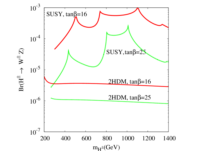
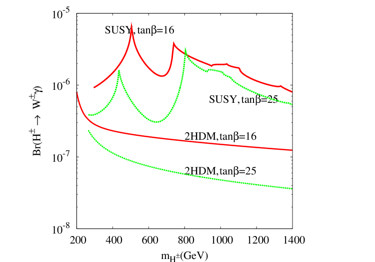
Figure 3: Branching ratios of $H^{\pm}\to W^{\pm}Z$ (left) and $H^{\pm}\to W^{\pm}\gamma$ (right) as a function of $m_{H^{\pm}}$ in the MSSM and 2HDM for $M_{SUSY}=500$ GeV, $M_{2}=175$ GeV, $\mu=-1.4$ GeV and $A_{t}=A_{b}=A_{\tau}=-\mu$ for various values of $\tan\beta$.

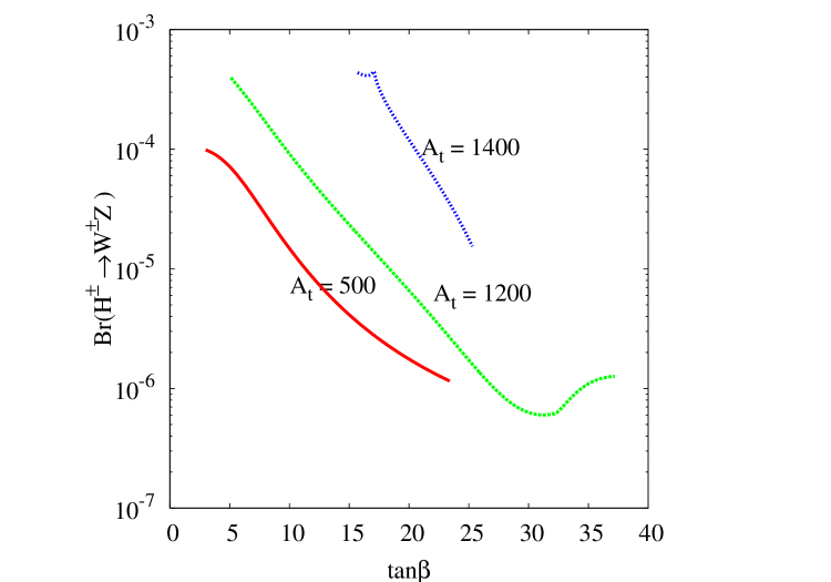
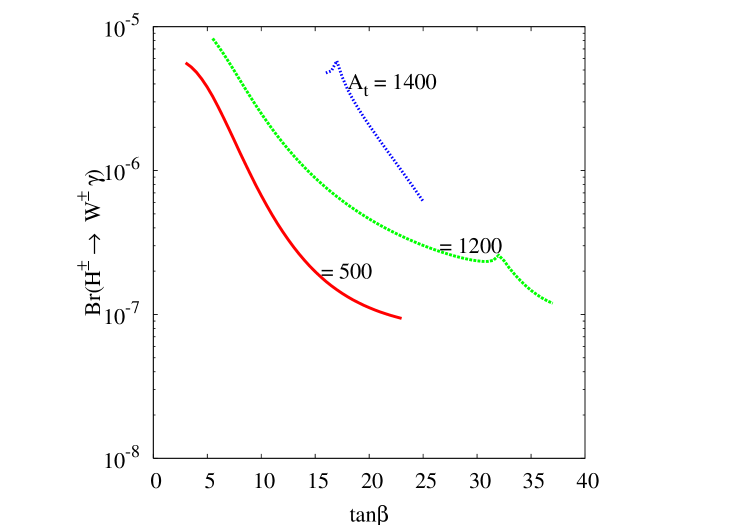
Figure 4: Branching ratios for $H^{\pm}\to W^{\pm}Z$ (left), $H^{\pm}\to W^{\pm}\gamma$ (right) as a function of $\tan\beta$ in the MSSM with $M_{SUSY}=500$ GeV, $M_{2}=200$ GeV, $m_{H^{\pm}}=500$ GeV, $A_{t}=A_{b}=A_{\tau}=-\mu$ for various values of $A_{t}$.

In Fig. 3, we show branching ratio of $H^{\pm}\to W^{\pm}Z$ (left) and $H^{\pm}\to W^{\pm}\gamma$ (right) as a function of charged Higgs mass for $\tan\beta=16$ and 25. In those plots, we have shown both the pure 2HDM (only SM fermion, gauge bosons and Higgs bosons with MSSM sum rules for the Higgs sector) and the MSSM (2HDM and SUSY particles) contribution. As it can be seen from those plots, both for $H^{\pm}\to W^{\pm}Z$ and $H^{\pm}\to W^{\pm}\gamma$ the 2HDM contribution is rather small. Once we include the SUSY particles, we can see that the Branching fraction get enhanced and can reach $10^{-3}$ in case of $H^{\pm}\to W^{\pm}Z$ and $10^{-5}$ in case of $H^{\pm}\to W^{\pm}\gamma$. The source of this enhancement is mainly due to the presence of scalar fermion contribution in the loop which are amplified by threshold effects from the opening of the decay $H^{\pm}\to\widetilde{t}_{i}\widetilde{b}_{j}^{*}$. It turns out that the contribution of charginos neutralinos loops does not enhance the Branching fraction significantly as compared to scalar fermions loops. The plots also show that, the branching fraction is more important for intermediate $\tan\beta=16$ and is slightly reduced for larger $\tan\beta=25$.

This $\tan\beta$ dependence is shown in Fig. 4 both for $H^{\pm}\to W^{\pm}Z$ and $H^{\pm}\to W^{\pm}\gamma$ for three representative values of $A_{t}$. It is obvious that the smallest is $\tan\beta$ the largest is the branching fraction. Increasing $\tan\beta$ from 5 to about 40 can reduce the branching fraction by about one or two order of magnitude.
We also show a scatter plot Fig. 5 for $H^{\pm}\to W^{\pm}Z$ (left) and $H^{\pm}\to W^{\pm}\gamma$ (right) in ($m_{H^{\pm}}$, $\tan\beta$) plane for $A_{t}=-\mu=1$ TeV, $M_{SUSY}=A_{t}$ and $M_{2}=175$ GeV. As it can be seen from Fig 5 there is only a small area for $\tan\beta\mathrel{\raise 1.29167pt\hbox{$<$\kern-7.5pt\lower 4.30554pt\hbox{$\sim$}}}10$ where the branching ratio of $H^{\pm}\to W^{\pm}Z$ can be in the range $10^{-5}$–$10^{-3}$.

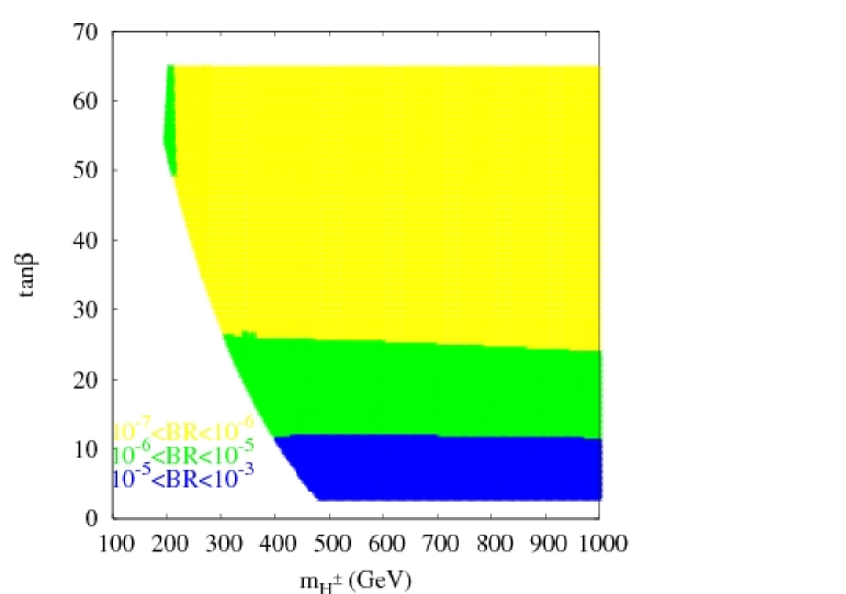
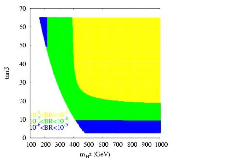
Figure 5: Scatter plot for branching ratios of $H^{\pm}\to W^{\pm}Z$ (left),$H^{\pm}\to W^{\pm}\gamma$ (right) in the ($m_{H^{\pm}}$, $\tan\beta$) plane in the MSSM for $M_{SUSY}=1$ TeV, $M_{2}=175$ GeV, $A_{t,b,\tau}=M_{SUSY}$ and $\mu=-1$ TeV.

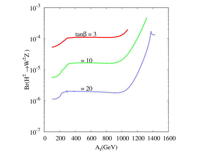
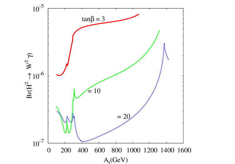
Figure 6: Branching ratios for $H^{\pm}\to W^{\pm}Z$ (left) and $H^{\pm}\to W^{\pm}\gamma$ (right) as a function of $A_{t}$ in the MSSM with $M_{SUSY}=500$ GeV, $M_{2}=200$ GeV, $m_{H^{\pm}}=500$ GeV, $A_{t}=A_{b}=A_{\tau}=-\mu$ and $-2\,\rm{TeV}<\mu<-0.1$ TeV for various values of $\tan\beta$.

We now illustrate in Fig. 6 the branching fraction of $H^{\pm}\to W^{\pm}Z$ (left) and $H^{\pm}\to W^{\pm}\gamma$ (right) as a function of $A_{t}=A_{b}=A_{\tau}=-\mu$ for $M_{SUSY}=500$ GeV and $M_{2}=200$ GeV. Since $b\to s\gamma$ favor $A_{t}$ and $\mu$ to have opposite sign, we fix $\mu=-A_{t}$ and in this sense also $\mu$ is varied when $A_{t}$ is varied. Both for $H^{\pm}\to W^{\pm}Z$ and $H^{\pm}\to W^{\pm}\gamma$, the chargino-neutralino contribution which is rather small decrease with $\mu=-A_{t}$, the largest is $A_{t}$ the smallest is chargino-neutralino contribution. In case of $H^{\pm}\to W^{\pm}Z$, for $A_{t}\mathrel{\raise 1.29167pt\hbox{$<$\kern-7.5pt\lower 4.30554pt\hbox{$\sim$}}}1$ TeV it is the pure 2HDM contribution which dominate and that is why it is almost independent of $A_{t}$ while for large $A_{t}$ the branching ratio increase with $A_{t}$. It is clear that the largest is $A_{t}$ the largest is the branching ratio which can be of the order of $10^{-3}$ for $H^{\pm}\to W^{\pm}Z$ with $\tan\beta=10$. As we know from $h^{0}\to\gamma\gamma$ and $h^{0}\to\gamma Z$ in MSSM whk , the squarks contributions decouple except in the light stop mass and large $A_{t}$ limit whk . In $H^{\pm}\to W^{\pm}V$ case, the same stuation happen. As we can see from Fig. 6 (left), for intermediate $A_{t}$, $300<A_{t}<1000$ GeV, the squarks are rather heavy and hence their contributions is small compared to 2HDM one. While for large $A_{t}$ the stop becomes very light $\mathrel{\raise 1.29167pt\hbox{$<$\kern-7.5pt\lower 4.30554pt\hbox{$\sim$}}}200$ GeV and hence enhance $H^{\pm}\to W^{\pm}V$ width. Of course this enhancement is also amplified by $H^{\pm}\widetilde{t}_{L,R}\widetilde{b}_{R,L}^{*}$ and $H^{\pm}\widetilde{\tau}_{L,R}\widetilde{\nu_{\tau}}_{L}^{*}$ couplings which are directly proportional to $A_{t,b,\tau}$. In case of $H^{\pm}\to W^{\pm}\gamma$ decay, the pure 2HDM and sfermions contributon are of comparable size, the branching ratio increases with $A_{t}$.

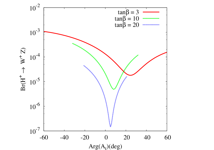
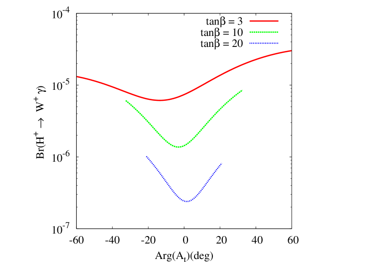
Figure 7: Branching ratios for $H^{\pm}\to W^{\pm}Z$ (left) and $H^{\pm}\to W^{\pm}\gamma$ (right) in the MSSM as a function of $Arg(A_{t})$ : $M_{SUSY}=500$ GeV, $M_{2}=150\,GeV$, $m_{H^{\pm}}=500$ GeV, $A_{t}=A_{b}=A_{\tau}=-\mu=1$ TeV and for various values of $\tan\beta$.

We have also studied the effect of the MSSM CP violating phases. It is well known that the presence of large SUSY CP violating phases can give contributions to electric dipole moments of the electron and neutron (EDM) which exceed the experimental upper bounds. In a variety of SUSY models such phases turn out to be severely constrained by such constraints i.e. ${\rm Arg}(\mu)<{\cal}(10^{-2})$ for a SUSY mass scale of the order of few hundred GeV nath . For $H^{\pm}\to W^{\pm}Z$ and $H^{\pm}\to W^{\pm}\gamma$ decays which are sensitive to MSSM CP violating phases through squarks and charginos-neutralinos contributions, it turns out that the effect of MSSM CP violating phases is important and can enhance the rate by about one order of magnitude. For illustration we show in Fig. 7 the effect of $A_{t,b,\tau}$ CP violating phases for $M_{SUSY}=500$ GeV, $A_{t,b,\tau}=-\mu=$ 1 TeV and $M_{2}=150$ GeV. For simplicity, we assume that $\mu$ is real. As it is clear, the CP phase of $A_{t,b,\tau}$ can enhance the rates of both $H^{\pm}\to W^{\pm}Z,\gamma$ by more than an ordre of magnitude. Those CP violating phases can lead to CP-violating rate asymmetry of $H^{\pm}$ decays, those issues are going to be addressed in an incoming paper prep .

We now turn to discuss the pure 2HDM contribution to $H^{\pm}\to W^{\pm}Z,W^{\pm}\gamma$. For the 2HDM parameterization we follow closely the notation of tch . In our discussion we will take as free parameters:

$$\lambda_{5}\quad,\quad m_{h^{0}}\quad,\quad m_{H^{0}}\quad,\quad m_{A^{0}}\quad,\quad m_{H\pm}\quad,\quad\tan\beta\quad{\rm and}\quad\sin\alpha$$ (15)

$\alpha$ is the CP-even mixing angle and $\lambda_{5}$ is the term that breaks softly the discrete symmetry $\Phi_{i}\to-\Phi_{i}$ in the 2HDM Lagrangian.

To constrain the scalar sector parameters we will use both vacuum stability conditions as well as tree level unitarity and $\delta\rho$ constraints. In our study, we use the vacuum stability conditions from vac1 and tree level unitarity constraints are taken from kan .
As $B\to X_{s}\gamma$ constraint is concerned, it has been shown in bsg that for models of the type 2HDM-II, data on $B\to X_{s}\gamma$ imposes a lower limit of $m_{H^{\pm}}\mathrel{\raise 1.29167pt\hbox{$>$\kern-7.5pt\lower 4.30554pt\hbox{$\sim$}}}350$ GeV. In type I 2HDM, there is no such constraint on the charged Higgs mass bsg . In our numerical analysis we will ignore these constraints and allow $m_{H\pm}\mathrel{\raise 1.29167pt\hbox{$<$\kern-7.5pt\lower 4.30554pt\hbox{$\sim$}}}200$ GeV in order to localize regions in parameter space where the branching ratios are sizeable.

In the 2HDM, the source of enhancement in $H^{\pm}\to W^{\pm}Z$ and $H^{\pm}\to W^{\pm}\gamma$ decays can be either from bottom Yukawa coupling which is enhanced at large $\tan\beta$ or from the Higgs sector contribution through diagram like Fig. 1.2 with $(S_{i},S_{j},S_{k})$=$(H^{\pm},h^{0},H^{\pm})$ or $(H^{\pm},H^{0},H^{\pm})$ and Fig. 1.8 with $(S_{i},S_{j})$=$(H^{\pm},h^{0})$ or $(H^{\pm},H^{0})$. In contrast to the MSSM where the trilinear scalar couplings $h^{0}H^{+}H^{-}$ and $H^{0}H^{+}H^{-}$ are function of the gauge couplings only, in the 2HDM those couplings are function of Higgs masses, $\alpha$, $\tan\beta$ as well as $\lambda_{5}$ as it can be seen from their analytic expressions (in the notations of Ref. tch )

$${H^{0}H^{+}H^{-}}= \frac{-ig}{m_{W}\sin 2\beta}(m_{H^{0}}^{2}(\cos^{3}\beta\sin\alpha+\sin^{3}\beta\cos\alpha)+m_{H^{\pm}}^{2}\sin{2\beta}\cos({\beta-\alpha})-\sin({\beta+\alpha})\lambda_{5}v^{2})$$

$${h^{0}H^{+}H^{-}}= \frac{-ig}{m_{W}\sin 2\beta}(m_{h^{0}}^{2}(\cos{\alpha}\cos^{3}{\beta}-\sin{\alpha}\sin^{3}{\beta})+m_{H^{\pm}}^{2}\sin{2\beta}\sin({\beta-\alpha})-\cos({\beta+\alpha}){\lambda_{5}}v^{2})$$ (16)

Even after imposing unitarity and vacuum stability constraints, those couplings can get large values compared to their MSSM values and that is the main difference between 2HDM scalar sector and the MSSM one.

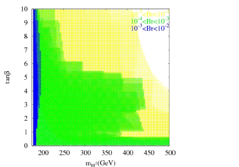
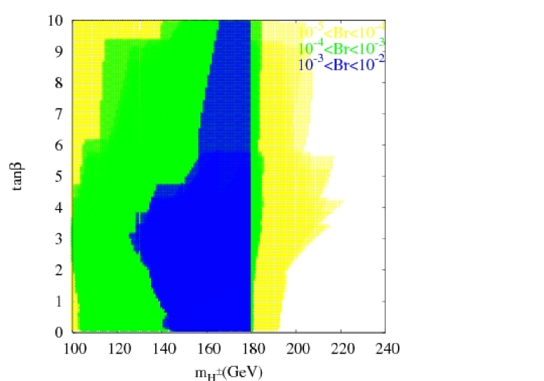
Figure 8: The branching ratios of $H^{\pm}\to W^{\pm}Z$ (left) and $H^{\pm}\to W^{\pm}\gamma$ (right) in type–II 2HDM model in ($m_{H^{\pm}},\tan\beta$) plane for $100\,\rm{GeV}\leq m_{h^{0}}\leq\,130\,\rm{GeV}$, $150\,\rm{GeV}\leq\,m_{H^{0}}\leq\,350\,\rm{GeV}$, $100\,\rm{GeV}\leq m_{A^{0},H^{\pm}}\leq 500$ GeV, $-1\leq\sin\alpha\leq 1$, $0.1\leq\tan\beta\leq 10$, and $\lambda_{5}=0$.

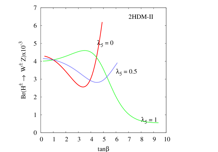
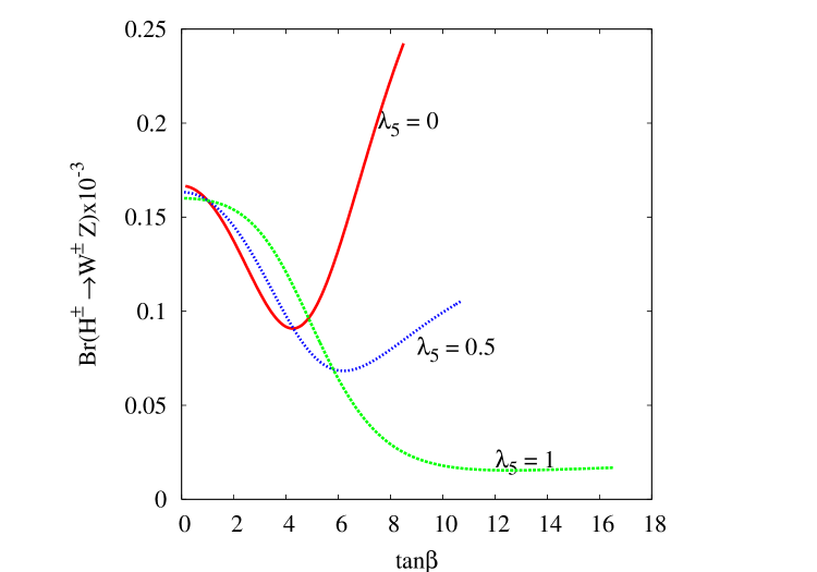
Figure 9: Branching ratios $H^{\pm}\to W^{\pm}Z$ as the function of the $\tan\beta$ in 2HDM-II for $m_{h^{0}}=100$ GeV, $m_{H^{0}}=200$ GeV, $m_{A^{0}}=300$ GeV $\alpha=\beta-\pi/2$ and various values of $\lambda_{5}$. Left plot is for $m_{H^{\pm}}=180$ GeV and right one is for $m_{H^{\pm}}=220$ GeV

We have first compared our results to previous one given in Refs. kanemur ; toscano and found perfect agreement. However in Refs. kanemur ; toscano , unitarity constraints were not imposed while Ref. toscano did not consider the case of $H^{\pm}\to W^{\pm}Z$. We have performed a systematic scan over the 2HDM parameters and found that both $H^{\pm}\to W^{\pm}Z$ and $H^{\pm}\to W^{\pm}\gamma$ can reach $10^{-2}$ branching ratio. In Fig.8 we have illustrated our results as scatter plot in the $(\tan\beta,m_{H^{\pm}})$ plane. As one can see from the plot, just before the opening of $H^{-}\to\bar{t}b$ decay, for $m_{H^{\pm}}\mathrel{\raise 1.29167pt\hbox{$<$\kern-7.5pt\lower 4.30554pt\hbox{$\sim$}}}m_{t}+m_{b}$, the branching ratio of $H^{\pm}\to W^{\pm}Z$ and $H^{\pm}\to W^{\pm}\gamma$ can be of the order $10^{-2}$–$10^{-3}$. Once the decay $H^{-}\to\bar{t}b$ is open for $m_{H^{\pm}}\mathrel{\raise 1.29167pt\hbox{$>$\kern-7.5pt\lower 4.30554pt\hbox{$\sim$}}}m_{t}+m_{b}$, the charged Higgs width becomes large and the branching ratio of $H^{\pm}\to W^{\pm}Z$ and $H^{\pm}\to W^{\pm}\gamma$ are suppressed. However as one can see, there is still a large area in the $(\tan\beta,m_{H^{\pm}})$ plane where the branching ratio of $H^{\pm}\to W^{\pm}Z$ and $H^{\pm}\to W^{\pm}\gamma$ can be larger than $10^{-4}$.

We illustrate in Fig. 9 the branching ratio of $H^{\pm}\to W^{\pm}Z$ as a function of $\tan\beta$ for various values of $\lambda_{5}$ and for $m_{H^{\pm}}=180$ GeV (left plot) and $m_{H^{\pm}}=220$ GeV (right plot). It is clear from both plots that the branching ratio is slightly enhanced for vanishing $\lambda_{5}$ case, this effect has been noticed also by kanemur . In the left plot we are very close to $H^{-}\to\bar{t}b$ threshold, the branching ratio is larger than $10^{-3}$. Away from the threshold $H^{-}\to\bar{t}b$ and for $m_{H^{\pm}}=220$ GeV (right plot) the branching ratio of $H^{\pm}\to W^{\pm}Z$ is slightly reduced to the level of $10^{-4}$.

IV Conclusion

In the framework of MSSM and 2HDM we have studied charged Higgs decays into a pair of gauge bosons namely: $H^{\pm}\to W^{\pm}Z$ and $H^{\pm}\to W^{\pm}\gamma$. In the MSSM we have also studied the effects of MSSM CP violating phases. In contrast to previous studies, we have performed the calculation in the ’tHooft-Feynman gauge and used a renormalization prescription to deal with tadpoles, $W^{\pm}$–$H^{\pm}$ and $G^{\pm}$–$H^{\pm}$ mixing. The study has been carried out taking into account the experimental constraint on the $\rho$ parameter, $b\to s\gamma$ constraint, unitarity constraints, and vacuum stability conditions on all scalar quartic couplings $\lambda_{i}$ in 2HDM case. Numerical results for the branching ratios have been presented. In the MSSM, we have shown that the branching ratio of $H^{\pm}\to W^{\pm}Z$ can reach $10^{-3}$ in some cases while $H^{\pm}\to W^{\pm}\gamma$ never exceed $10^{-5}$. The effect of MSSM CP violating phases is also found to be important.
In the 2HDM we emphasize the effect coming from the pure trilinear scalar couplings such as $h^{0}H^{+}H^{-}$ and $H^{0}H^{+}H^{-}$. We have shown that in 2HDM both $H^{\pm}\to W^{\pm}Z$ and $H^{\pm}\to W^{\pm}\gamma$ can have a branching ratio in the range $10^{-2}$–$10^{-3}$.
Those Branching ratio in the range $10^{-2}$–$10^{-3}$ might provide an opportunity to search for a charged Higgs boson at the LHC through $H^{\pm}\to W^{\pm}Z$.

Appendix A Lagrangian and couplings

In this appendix, we list our notation for the gauge and Yukawa couplings used in this section.

The photon coupling to fermions/sfermions are:

$$g_{\gamma ff}^{L,R}=-e_{f}s_{W},\ \ \ g_{\gamma\tilde{f}_{i}\tilde{f}_{j}}=-e_{f}s_{W}\delta_{ij}$$ (17)

The $Z$ boson coupling to fermions/sfermions are:

$$g_{Zff}^{L} = (-T_{3}+e_{f}s_{W}^{2})/c_{W},\ \ \ g_{Zff}^{R}=e_{f}s_{W}^{2}/c_{W}$$ (18)

$$g_{Z\tilde{f}_{i}\tilde{f}_{j}} = c_{ij}/c_{W}$$ (19)

where the couplings $c_{ij}$ are given by

$$c_{ij}=\left(\begin{array}[]{cc}T_{3}\cos^{2}_{\theta_{f}}-e_{f}s_{W}^{2}&-\frac{1}{2}T_{3}\sin 2\theta_{f}\\ -\frac{1}{2}T_{3}\sin 2\theta_{f}&T_{3}\sin^{2}_{\theta_{f}}-e_{f}s_{W}^{2}\end{array}\right)$$ (20)

where $T_{3}=1/2$ for up quarks and $T_{3}=-1/2$ for down quarks and $\theta_{f}$ is the mixing angle in the sfermion sector defined by:

$$\left(\begin{array}[]{c}\tilde{f}_{L}\\ \tilde{f}_{R}\end{array}\right)=\left(\begin{array}[]{cc}\cos\theta_{f}&-\sin\theta_{f}\\ \sin\theta_{f}&\cos\theta_{f}\end{array}\right)\left(\begin{array}[]{c}\tilde{f}_{1}\\ \tilde{f}_{2}\end{array}\right)=R^{f}_{ij}\left(\begin{array}[]{c}\tilde{f}_{1}\\ \tilde{f}_{2}\end{array}\right)$$ (21)

where $\tilde{f}_{L,R}$ are the weak eigenstates and $\tilde{f}_{1,2}$ are the mass eigenstates.

The $W$ gauge boson coupling to a pair of fermions/sfermions is:

$$g_{Wff^{\prime}}^{L} = -\frac{1}{\sqrt{2}},\ \ \ g_{Wff^{\prime}}^{R}=0$$ (22)

$$g_{W\tilde{f}_{i}\tilde{f}_{j}} = -\frac{1}{\sqrt{2}}R^{f}_{i1}R^{f^{\prime}}_{j1}$$ (23)

The chargino mass matrix is:

$$X=\left(\begin{array}[]{cc}M_{2}&\sqrt{2}m_{W}\sin\beta\\ \sqrt{2}m_{W}\cos\beta&\mu\end{array}\right),$$ (24)

which is diagonalized by the unitary matrices $U$ and $V$ via $VX^{\dagger}U^{\dagger}=M_{D}$.

The neutralino mass matrix is:

$$Y=\left(\begin{array}[]{cccc}M_{1}&0&-m_{Z}s_{W}\cos\beta&m_{Z}s_{W}\sin\beta\\ 0&M_{2}&m_{Z}c_{W}\cos\beta&-m_{Z}c_{W}\sin\beta\\ -m_{Z}s_{W}\cos\beta&m_{Z}c_{W}\cos\beta&0&-\mu\\ m_{Z}s_{W}\sin\beta&-m_{Z}c_{W}\sin\beta&-\mu&0\end{array}\right),$$ (25)

which is diagonalized by the matrix $N$ via $NY^{\dagger}N^{\dagger}=N_{D}$.

The matrices that enter the $W^{\pm}\tilde{\chi}_{i}^{0}\tilde{\chi}_{j}^{\mp}$ couplings are defined as:

$${\cal O}_{ij}^{L}=-\frac{1}{\sqrt{2}}N_{i4}V_{j2}^{*}+N_{i2}V_{j1}^{*},\ \ \ {\cal O}_{ij}^{R}=\frac{1}{\sqrt{2}}N_{i3}^{*}U_{j2}+N_{i2}^{*}U_{j1}.$$ (26)

The matrices that enter the $Z\tilde{\chi}_{i}^{\pm}\tilde{\chi}_{j}^{\mp}$ couplings are defined as:

$${\cal O}_{ij}^{\prime{L}} = -V_{i1}V_{j1}^{*}-\frac{1}{2}V_{i2}V_{j2}^{*}+\delta_{ij}s_{W}^{2},$$

$${\cal O}_{ij}^{\prime{R}} = -U_{i1}^{*}U_{j1}-\frac{1}{2}U_{i2}^{*}U_{j2}+\delta_{ij}s_{W}^{2}.$$ (27)

The matrices that enter the $Z\tilde{\chi}_{i}^{0}\tilde{\chi}_{j}^{0}$ couplings are defined as:

$${\cal O}_{ij}^{\prime\prime{L}}=-\frac{1}{2}N_{i3}N_{j3}^{*}+\frac{1}{2}N_{i4}N_{j4}^{*},\ \ \ {\cal O}_{ij}^{\prime\prime{R}}=-O_{ij}^{\prime\prime{L}*}.$$ (28)

The matrices that enter the $H^{\mp}\tilde{\chi}_{i}^{0}\tilde{\chi}_{j}^{\pm}$ and $H^{\mp}u_{j}d_{j}$ couplings are defined as:

$${\cal O}_{ij}^{\prime{L}} = N_{i4}^{*}V_{j1}^{*}+\frac{1}{\sqrt{2}}(N_{i2}^{*}+N_{i1}^{*}\tan\theta_{W})V_{j2}^{*},$$

$${\cal O}_{ij}^{\prime{R}} = N_{i3}U_{j1}-\frac{1}{\sqrt{2}}(N_{i2}+N_{i1}\tan\theta_{W})U_{j2}.$$

$$g_{H^{\pm}u_{i}d_{i}}^{L,R} = \frac{(m_{d_{i}}\tan\beta,m_{u_{i}}/\tan\beta)}{\sqrt{2}m_{W}},\ \ \ g_{G^{\pm}u_{i}d_{i}}^{L,R}=\frac{m_{u_{i}},m_{d_{i}}}{\sqrt{2}m_{W}}$$ (29)

The couplings $W^{\pm}G^{\mp}V$, $W^{\pm}W^{\mp}V$ and $H^{\pm}H^{\mp}V$ are given:

$V$	$g_{WGV}$	$g_{WWV}$	$g_{HHV}$
$Z$	$-m_{Z}s_{W}^{2}$	$c_{W}$	$(c_{W}^{2}-s_{W}^{2})/2c_{W}$
$\gamma$	$m_{W}s_{W}$	$-s_{W}$	$s_{W}$

The coupling $H^{\mp}\tilde{f}\tilde{f}^{\prime}$ are given by

$$g_{H{\tilde{e}}_{L}{\tilde{\nu}}} = -m_{W}\sin{2}\beta/\sqrt{2}$$

$$g_{H{\tilde{d}}_{L}{\tilde{u}}_{L}} = -m_{W}\sin{2}\beta/\sqrt{2}$$

$$g_{H^{-}{\tilde{b}}_{L}{\tilde{t}}_{L}} = -m_{W}\sin{2}\beta/\sqrt{2}+(m_{b}^{2}\tan\beta+m_{t}^{2}\cot\beta)/\sqrt{2}m_{W}$$

$$g_{H^{-}{\tilde{b}}_{L}{\tilde{t}}_{R}} = m_{t}(\mu+A_{t}\cot\beta)/\sqrt{2}m_{W}$$

$$g_{H^{-}{\tilde{b}}_{R}{\tilde{t}}_{L}} = m_{b}(\mu+A_{b}\tan\beta)/\sqrt{2}m_{W}$$

$$g_{H^{-}{\tilde{b}}_{R}{\tilde{t}}_{R}} = m_{t}m_{b}(\tan\beta+\cot\beta)/\sqrt{2}m_{W}$$ (30)

$$g_{H{\tilde{b}}_{1}{\tilde{t}}_{1}} = c_{\theta_{t}}c_{\theta_{b}}{g}_{H^{-}{\tilde{b}}_{L}{\tilde{t}}_{L}}+s_{\theta_{t}}c_{\theta_{b}}{g}_{H^{-}{\tilde{b}}_{L}{\tilde{t}}_{R}}+c_{\theta_{t}}s_{\theta_{b}}{g}_{H^{-}{\tilde{b}}_{R}{\tilde{t}}_{L}}+s_{\theta_{t}}s_{\theta_{b}}{g}_{H^{-}{\tilde{b}}_{R}{\tilde{t}}_{R}}$$

$$g_{H{\tilde{b}}_{1}{\tilde{t}}_{2}} = -s_{\theta_{t}}c_{\theta_{b}}{g}_{H^{-}{\tilde{b}}_{L}{\tilde{t}}_{L}}+c_{\theta_{t}}c_{\theta_{b}}{g}_{H^{-}{\tilde{b}}_{L}{\tilde{t}}_{R}}-s_{\theta_{t}}s_{\theta_{b}}{g}_{H^{-}{\tilde{b}}_{R}{\tilde{t}}_{L}}+c_{\theta_{t}}s_{\theta_{b}}{g}_{H^{-}{\tilde{b}}_{R}{\tilde{t}}_{R}}$$

$$g_{H{\tilde{b}}_{2}{\tilde{t}}_{1}} = -c_{\theta_{t}}s_{\theta_{b}}{g}_{H^{-}{\tilde{b}}_{L}{\tilde{t}}_{L}}-s_{\theta_{t}}s_{\theta_{b}}{g}_{H^{-}{\tilde{b}}_{L}{\tilde{t}}_{R}}+c_{\theta_{t}}c_{\theta_{b}}{g}_{H^{-}{\tilde{b}}_{R}{\tilde{t}}_{L}}+s_{\theta_{t}}c_{\theta_{b}}{g}_{H^{-}{\tilde{b}}_{R}{\tilde{t}}_{R}}$$

$$g_{H{\tilde{b}}_{2}{\tilde{t}}_{2}} = s_{\theta_{t}}s_{\theta_{b}}{g}_{H^{-}{\tilde{b}}_{L}{\tilde{t}}_{L}}-c_{\theta_{t}}s_{\theta_{b}}{g}_{H^{-}{\tilde{b}}_{L}{\tilde{t}}_{R}}-s_{\theta_{t}}c_{\theta_{b}}{g}_{H^{-}{\tilde{b}}_{R}{\tilde{t}}_{L}}+c_{\theta_{t}}c_{\theta_{b}}{g}_{H^{-}{\tilde{b}}_{R}{\tilde{t}}_{R}}$$ (31)

Appendix B MSSM contribution for $H^{\pm}\to W^{\pm}V$

We now list our results for the MSSM diagrams. The matrix elements for $H^{\pm}\to W^{\pm}V$ ($V=Z,\gamma$) in the MSSM are partially presented here. We give only the fermionic contribution (SM fermion and chargino-neutralino contribution) as well as the scalar fermion contributions. For the bosonic contribution (higgs bosons and gauge bosons) we refer to kanemur .
It is to be understood that diagrams involving charginos $\tilde{\chi}^{\pm}_{i}$ are summed over $i=1,2$ and diagrams involving neutralinos $\tilde{\chi}^{0}_{i}$ are summed over $i=1,\ldots,4$.
The fermion triangle that enters Fig. 1.1a and Fig. 1.1b was computed in Ref. micapey , and agrees with our result. Fig. 1.1c with $\tilde{\chi}_{i}^{0}$, $\tilde{\chi}_{j}^{0}$ and $\tilde{\chi}_{k}^{\pm}$ in the loop is analogous to the top/bottom quark triangle diagram and can be checked by substituting top/bottom quark couplings into the gaugino couplings.

Diagram Fig. 1.1a: In the convention of eq.2, we have

$${\cal F}_{1} = N_{C}g^{L}_{W}\Big{(}2(m_{t}g^{L}_{Vbb}g^{R}_{H}+m_{b}g^{L}_{Vbb}g^{L}_{H}-m_{b}g^{R}_{Vbb}g^{L}_{H})B_{0}-2m_{t}m_{b}g^{R}_{Vbb}(m_{t}g^{L}_{H}+m_{b}g^{R}_{H})C_{0}$$

$$+ \Big{[}-m_{b}g^{R}_{Vbb}g^{L}_{H}(m_{H^{\pm}}^{2}+m_{W}^{2}-m^{2}_{V})-m_{t}g^{L}_{Vbb}g^{R}_{H}(-m_{H^{\pm}}^{2}-3m_{W}^{2}+m^{2}_{V})+2m_{b}g^{L}_{Vbb}g^{R}_{H}m_{W}^{2}\Big{]}C_{1}$$

$$+ \Big{[}m_{t}g^{L}_{Vbb}g^{R}_{H}(3m_{H^{\pm}}^{2}+m_{W}^{2}-m^{2}_{V})+m_{b}g^{L}_{Vbb}g^{L}_{H}(m_{H^{\pm}}^{2}+m_{W}^{2}-m^{2}_{V})-2g^{R}_{Vbb}g^{L}_{H}m_{H^{\pm}}^{2}m_{b}\Big{]}C_{2}$$

$$- 4g^{L}_{Vbb}(m_{t}g^{R}_{H}+m_{b}g^{L}_{H})C_{00}\Big{)}$$

$${\cal F}_{2} = -2N_{C}g^{L}_{W}\Big{(}m_{t}g^{L}_{Vbb}g^{R}_{H}\,C_{0}-(m_{t}g^{L}_{Vbb}g^{R}_{H}-m_{b}g^{R}_{Vbb}g^{R}_{H})\,C_{1}+3g^{L}_{Vbb}(m_{t}g^{R}_{H}+m_{b}g^{L}_{H})\,C_{2}\Big{)}$$ (33)

$${\cal F}_{3} = 2N_{C}g^{L}_{W}\Big{(}m_{t}g^{L}_{Vbb}g^{R}_{H}\,C_{0}+(m_{t}g^{L}_{Vbb}g^{R}_{H}+m_{b}g^{R}_{Vbb}g^{L}_{H})\,C_{1}+g^{L}_{Vbb}(m_{t}g^{R}_{H}+m_{b}g^{L}_{H})\,C_{2}\Big{)}$$ (34)

Where $N_{C}=3$ for quarks and 1 for leptons. The arguments of the Passarino-Veltman functions $B_{i}$ and $C_{i}$ are $B_{i}(m^{2}_{V},m^{2}_{b},m^{2}_{b})$, $C_{i}(m^{2}_{W},m^{2}_{V},m_{H^{\pm}}^{2},m^{2}_{t},m^{2}_{b},m^{2}_{b})$.

Diagram Fig. 1.1b:

Similar to Fig. 1.1(a) with the exchange of

$$m_{t}\leftrightarrow m_{b},\ \ \ g^{R}_{Vtt}\leftrightarrow g^{R}_{Vbb},\ \ \ g^{L}_{Vtt}\leftrightarrow g^{L}_{Vbb},\ \ \ g^{L}_{H}\leftrightarrow g^{R}_{H},\ \ \ g^{L}_{W}\leftrightarrow g^{L*}_{W}$$ (35)

Diagram Fig. 1.1c

$${\cal F}_{1} = \Big{(}2\Big{[}m_{\chi_{i}}(g_{1}g_{3}g_{5}+g_{2}g_{4}g_{6})+m_{\chi_{j}}(g_{1}g_{3}g_{6}+g_{2}g_{4}g_{5})-m_{\chi_{k}}(g_{1}g_{4}g_{5}+g_{2}g_{3}g_{6})\Big{]}\,B_{0}$$

$$+ \Big{[}m_{\chi_{i}}(-2g_{1}g_{4}g_{5}m_{\chi_{i}}m_{\chi_{k}}-2g_{1}g_{4}g_{6}m_{\chi_{j}}m_{\chi_{k}}+2g_{1}g_{3}g_{6}m_{\chi_{i}}m_{\chi_{j}}+2g_{1}g_{3}g_{5}m_{\chi_{i}}^{2}$$

$$+g_{1}g_{3}g_{5}(m_{H^{\pm}}^{2}+m_{W}^{2}-m_{V}^{2}))\Big{]}\,C_{0}+\Big{[}-m_{\chi_{k}}(g_{1}g_{4}g_{5}+g_{2}g_{3}g_{6})(m_{H^{\pm}}^{2}+m_{W}^{2}-m_{V}^{2})$$

$$+m_{\chi_{i}}(g_{1}g_{3}g_{5}-g_{2}g_{4}g_{6})(-m_{H^{\pm}}^{2}-3m_{W}^{2}+m_{V}^{2})-2(g_{1}g_{3}g_{6}-g_{2}g_{4}g_{5})m_{\chi_{j}}m_{W}^{2}\Big{]}\,C_{1}$$

$$+ \Big{[}m_{\chi_{i}}(g_{1}g_{3}g_{5}+g_{2}g_{4}g_{6})(3m_{H^{\pm}}^{2}+m_{W}^{2}-m_{V}^{2})+m_{\chi_{j}}(g_{2}g_{4}g_{5}+g_{1}g_{3}g_{6})(m_{H^{\pm}}^{2}+m_{W}^{2}-m_{V}^{2})$$

$$-2(g_{1}g_{4}g_{5}-g_{2}g_{3}g_{5})m_{\chi_{k}}m_{H^{\pm}}^{2}\Big{]}\,C_{2}$$

$$- 4\Big{[}m_{\chi_{i}}(g_{1}g_{3}g_{5}+g_{2}g_{4}g_{6})+m_{\chi_{j}}(g_{1}g_{3}g_{6}+g_{2}g_{4}g_{5})\Big{]}\,C_{00}\Big{)}$$

$${\cal F}_{2} = -2\Big{(}(m_{\chi_{i}}(g_{1}g_{3}g_{5}+g_{2}g_{4}g_{6}))\,C_{0}-\Big{[}m_{\chi_{k}}(g_{2}g_{3}g_{6}-g_{1}g_{4}g_{5})+m_{\chi_{i}}(g_{1}g_{3}g_{5}+g_{2}g_{4}g_{6})\Big{]}\,C_{1}$$

$$+ 3\Big{[}m_{\chi_{i}}(g_{1}g_{3}g_{5}+g_{2}g_{4}g_{6})+m_{\chi_{j}}(g_{1}g_{3}g_{6}+g_{2}g_{4}g_{5})\Big{]}\,C_{2}\Big{)}$$

$${\cal F}_{3} = 8\Big{(}m_{\chi_{i}}(g_{1}g_{3}g_{5}-g_{2}g_{4}g_{6})\,C_{0}+\Big{[}m_{\chi_{k}}(g_{2}g_{3}g_{6}-g_{1}g_{4}g_{5})+m_{\chi_{i}}(g_{1}g_{3}g_{5}-g_{2}g_{4}g_{6})\Big{]}\,C_{1}$$

$$+ \Big{[}m_{\chi_{i}}(g_{1}g_{3}g_{5}-g_{2}g_{4}g_{6})-m_{\chi_{j}}(g_{2}g_{4}g_{5}-g_{1}g_{3}g_{6})\Big{]}\,C_{2}\Big{)}$$

The arguments of $B_{i}$ and $C_{i}$ functions are $B_{i}(m^{2}_{V},m^{2}_{\chi_{i}},m^{2}_{\chi_{j}})$, $C_{i}(m^{2}_{W},m^{2}_{V},m_{H^{\pm}}^{2},m^{2}_{\chi_{i}},m^{2}_{\chi_{k}},m^{2}_{\chi_{j}})$. The couplings are given in the following table:

$\chi_{i}$	$\chi_{j}$	$\chi_{k}$	$g_{1}$	$g_{2}$	$g_{3}$	$g_{4}$	$g_{5}$	$g_{6}$
$\tilde{\chi}^{0}$	$\tilde{\chi}^{0}$	$\tilde{\chi}^{+}$	$2\,{\cal O}_{ij}^{\prime\prime{L}}/c_{W}$	$-2\,{\cal O}_{ij}^{\prime\prime{R}}/c_{W}$	$-\,{\cal O}_{kj}^{R*}$	$-\,{\cal O}_{kj}^{L*}$	$-\,c_{\beta}\,{\cal O}_{ki}^{\prime{L}}$	$-\,s_{\beta}\,{\cal O}_{ki}^{\prime{R}}$
$\tilde{\chi}^{+}$	$\tilde{\chi}^{-}$	$\tilde{\chi}^{0}$	$\,{\cal O}_{ij}^{\prime{L}}/c_{W}$	$\,{\cal O}_{ij}^{\prime{R}}/c_{W}$	$-\,{\cal O}_{kj}^{R*}$	$-\,{\cal O}_{kj}^{L*}$	$-\,c_{\beta}\,{\cal O}_{ki}^{\prime{L}}$	$-\,s_{\beta}\,{\cal O}_{ki}^{\prime{R}}$

Diagram Fig. 1.2:

$${\cal{F}}_{1} = 4\,N_{C}\,g_{1}^{V}g_{2}^{H}g_{3}^{W}\,C_{00}$$ (39)

$${\cal{F}}_{2} = N_{C}\,g_{1}^{V}g_{2}^{H}g_{3}^{W}\,\Big{(}C_{0}+2(C_{1}+2C_{12}+C_{2})\Big{)}$$ (40)

Where $N_{C}=3$ for scalar quarks and $N_{C}=1$ for scalar leptons, the arguments of $C_{i}$ and $C_{ij}$ functions are as $C_{i,ij}(m^{2}_{W},m^{2}_{V},m^{2}_{S_{i}},m^{2}_{S_{k}},m^{2}_{S_{j}})$. The couplings are given in the following table:

$S_{i}$	$S_{j}$	$S_{k}$	$g_{1}^{\gamma}$	$g_{1}^{Z}$	$g_{2}^{H}$	$g_{3}^{W}$
${\tilde{\nu}}_{l}$	${\tilde{\nu}}_{l}$	$\tilde{l}_{L}$	$-g_{\gamma{\tilde{\nu}}{\tilde{\nu}}}$	$-g_{Z{\tilde{\nu}}{\tilde{\nu}}}$	$g_{H{\tilde{\nu}}\tilde{l}}$	$g_{W{\tilde{\nu}}\tilde{l}}$
$\tilde{l}_{L}$	$\tilde{l}_{L}$	${\tilde{\nu}}_{l}$	$g_{\gamma\tilde{l}\tilde{l}}$	$g_{Z\tilde{l}\tilde{l}}$	$g_{H\tilde{l}{\tilde{\nu}}}$	$g_{W\tilde{l}{\tilde{\nu}}}$
$\tilde{u}_{L}$	$\tilde{u}_{L}$	$\tilde{d}_{L}$	$-g_{\gamma\tilde{u}\tilde{u}}$	$-g_{Z\tilde{u}\tilde{u}}$	$g_{H\tilde{u}\tilde{d}}$	$g_{W\tilde{u}\tilde{d}}$
$\tilde{d}_{L}$	$\tilde{d}_{L}$	$\tilde{u}_{L}$	$g_{\gamma\tilde{d}\tilde{d}}$	$g_{Z\tilde{d}\tilde{d}}$	$g_{H\tilde{d}\tilde{u}}$	$g_{W\tilde{d}\tilde{u}}$
$\tilde{t}_{i}$	$\tilde{t}_{j}$	$\tilde{b}_{k}$	$-g_{\gamma}^{uL}{R}^{t}_{1i}{R}^{t}_{1j}-g_{\gamma}^{uR}{R}^{t}_{2i}{R}^{t}_{2j}$	$-g_{Z}^{uL}{R}^{t}_{1i}{R}^{t}_{1j}-g_{Z}^{uR}{R}^{t}_{2i}{R}^{t}_{2j}$	$g_{H\tilde{b}\tilde{t}}$	$-{R}^{t}_{1j}{R}^{b}_{1k}$
$\tilde{b}_{i}$	$\tilde{b}_{i}$	$\tilde{t}_{k}$	$g_{\gamma}^{dL}{R}^{b}_{1i}{R}^{b}_{1j}+g_{\gamma}^{dR}{R}^{b}_{2i}{R}^{b}_{2j}$	$g_{Z}^{dL}{R}^{b}_{1i}{R}^{b}_{1j}+g_{Z}^{dR}{R}^{b}_{2i}{R}^{b}_{2j}$	$g_{H\tilde{b}\tilde{t}}$	${R}^{t}_{1k}{R}^{b}_{1j}$

where $R^{t,b}_{11}=R^{t,b}_{22}=\cos\theta_{f}$ and $-R^{t,b}_{12}=R^{t,b}_{21}=\sin\theta_{f}$.

Diagram Fig. 1.8:

$${\cal{F}}_{1} = -N_{C}g_{1}g_{2}B_{0}(m_{H^{\pm}}^{2},m_{S_{i}}^{2},m_{S_{j}}^{2})$$ (41)

The couplings are given in the following table:

$S_{i}$	$S_{j}$	$g_{1}$	$g_{2}$
$\tilde{\nu}_{l}$	$\tilde{l}_{L}$	$g_{H^{\pm}{\tilde{\nu}}_{l}\tilde{l}_{L}}$	$g_{{\tilde{\nu}}\tilde{l}_{L}W^{\pm}V}$
$\tilde{t}_{L}$	$\tilde{b}_{L}$	$g_{H^{\pm}\tilde{t}_{L}\tilde{b}_{L}}$	$g_{\tilde{t}_{L}\tilde{b}_{L}W^{\pm}V}$
$\tilde{t}_{1}$	$\tilde{b}_{1}$	$g_{H^{\pm}\tilde{t}_{1}\tilde{b}_{1}}$	$g_{\tilde{t}_{1}\tilde{b}_{1}W^{\pm}V}$
$\tilde{t}_{1}$	$\tilde{b}_{2}$	$g_{H^{\pm}\tilde{t}_{1}\tilde{b}_{2}}$	$g_{\tilde{t}_{1}\tilde{b}_{2}W^{\pm}V}$
$\tilde{t}_{2}$	$\tilde{b}_{1}$	$g_{H^{\pm}\tilde{t}_{2}\tilde{b}_{1}}$	$g_{\tilde{t}_{2}\tilde{b}_{1}W^{\pm}V}$
$\tilde{t}_{2}$	$\tilde{b}_{2}$	$g_{H^{\pm}\tilde{t}_{2}\tilde{b}_{2}}$	$g_{\tilde{t}_{2}\tilde{b}_{2}W^{\pm}V}$

Diagram Fig. 1.12:

$${\cal{F}}_{2} = \frac{2\,N_{C}\,g_{3}}{m_{W}^{2}-m_{H^{\pm}}^{2}}\Big{(}-m_{F_{i}}(g_{1}g_{4}+g_{2}g_{5})B_{0}+\Big{[}(g_{1}g_{4}+g_{2}g_{5})m_{F_{i}}+(g_{2}g_{4}+g_{1}g_{5})m_{F_{j}}\Big{]}B_{1}\Big{)}$$ (42)

The arguments for the Passarino-Veltman functions $B_{i}$ are $B_{i}(m_{V}^{2},m^{2}_{F_{i}},m^{2}_{F_{j}})$.

The couplings are given in the following table:

$F_{i}$	$F_{j}$	$S_{k}$	$g_{1}$	$g_{2}$	$g_{3}$	$g_{4}$	$g_{5}$
$t$	$b$	$H^{\pm}$	$0$	$g_{W^{\pm}tb}^{L}$	$g_{H^{\pm}W^{\pm}V}$	$g_{H^{\pm}tb}^{L}$	$g_{H^{\mp}tb}^{R}$
$\tilde{\chi}^{0}$	$\tilde{\chi}^{+}$	$H^{\pm}$	${\cal O}^{L*}_{ji}$	${\cal O}^{R*}_{ji}$	$g_{H^{\pm}W^{\pm}V}$	$-c_{\beta}{\cal O}^{\prime L}_{ji}$	$-s_{\beta}{\cal O}^{\prime R}_{ji}$

Diagram Fig. 1.13:

$${\cal{F}}_{2}=\frac{N_{C}\,g_{1}\,g_{2}\,g_{3}}{m_{W}^{2}-m_{H^{\pm}}^{2}}\Big{(}B_{0}(m_{W}^{2},m_{S_{j}}^{2},m_{S_{i}}^{2})+2B_{1}(m_{W}^{2},m_{S_{j}}^{2},m_{S_{i}}^{2})\Big{)}$$ (43)

The couplings are given in the following table:

$S_{i}$	$S_{j}$	$S_{k}$	$g_{1}$	$g_{2}$	$g_{3}$
$\tilde{\nu}_{l}$	$\tilde{l}_{L}$	$H^{\pm}$	$g_{H^{\pm}H^{\mp}V}$	$g_{H^{\pm}{\tilde{\nu}}_{l}\tilde{l}_{L}}$	$g_{{\tilde{\nu}}_{l}\tilde{l}_{L}W^{\pm}}$
$\tilde{u}_{L}$	$\tilde{d}_{L}$	$H^{\pm}$	$g_{H^{\pm}H^{\mp}V}$	$g_{H^{\pm}\tilde{u}_{L}\tilde{d}_{L}}$	$g_{\tilde{u}_{L}\tilde{d}_{L}W^{\pm}}$
$\tilde{t}_{1}$	$\tilde{b}_{1}$	$H^{\pm}$	$g_{H^{\pm}H^{\mp}V}$	$g_{H^{\pm}\tilde{t}_{1}\tilde{b}_{1}}$	$g_{\tilde{t}_{1}\tilde{b}_{1}W^{\pm}}$
$\tilde{t}_{1}$	$\tilde{b}_{2}$	$H^{\pm}$	$g_{H^{\pm}H^{\mp}V}$	$g_{H^{\pm}\tilde{t}_{1}\tilde{b}_{2}}$	$g_{\tilde{t}_{1}\tilde{b}_{2}W^{\pm}}$
$\tilde{t}_{2}$	$\tilde{b}_{1}$	$H^{\pm}$	$g_{H^{\pm}H^{\mp}V}$	$g_{H^{\pm}\tilde{t}_{2}\tilde{b}_{1}}$	$g_{\tilde{t}_{2}\tilde{b}_{1}W^{\pm}}$
$\tilde{t}_{2}$	$\tilde{b}_{2}$	$H^{\pm}$	$g_{H^{\pm}H^{\mp}V}$	$g_{H^{\pm}\tilde{t}_{2}\tilde{b}_{2}}$	$g_{\tilde{t}_{2}\tilde{b}_{2}W^{\pm}}$

Diagram Fig. 1.15:

$${\cal{F}}_{1} = \frac{2\,N_{C}\,g_{5}}{m_{H^{\pm}}^{2}-m_{W}^{2}}\Big{(}(g_{2}g_{3}+g_{1}g_{4})\,A_{0}(m_{F_{j}}^{2})+m_{F_{i}}\Big{[}(g_{2}g_{3}+g_{1}g_{4})m_{F_{i}}+(g_{1}g_{3}+g_{2}g_{4})m_{F_{j}}\Big{]}B_{0}$$

$$+ (g_{2}g_{3}+g_{1}g_{4})g_{5}m_{H^{\pm}}^{2}B_{1}\Big{)}$$

The arguments of $B_{i}$ functions are $B_{i}(m_{H^{\pm}}^{2},m^{2}_{F_{i}},m^{2}_{F_{j}})$. The couplings are given in the following table:

$F_{i}$	$F_{j}$	$S_{k}$	$g_{1}$	$g_{2}$	$g_{3}$	$g_{4}$	$g_{5}$
$t$	$b$	$G^{\pm}$	$g_{G^{\pm}tb}^{L}$	$g_{G^{\pm}tb}^{R}$	$g_{G\pm W^{\pm}V}$	$g_{H^{\pm}tb}^{L}$	$g_{H^{\mp}tb}^{R}$
$\tilde{\chi}^{0}$	$\tilde{\chi}^{+}$	$G^{\pm}$	$-c_{\beta}{\cal O}^{\prime L}_{ji}$	$-s_{\beta}{\cal O}^{\prime R}_{ji}$	$g_{G^{\pm}W^{\mp}V}$	$c_{\beta}{\cal O}^{\prime R*}_{ji}$	$-s_{\beta}{\cal O}^{\prime L*}_{ji}$

Diagram Fig. 1.16:

$${\cal{F}}_{1}=\frac{N_{C}g_{1}g_{2}g_{3}}{m_{H^{\pm}}^{2}-m_{S_{k}}^{2}}B_{0}(m_{H^{\pm}}^{2},m_{S_{j}}^{2},m_{S_{i}}^{2})$$ (45)

The couplings are given in the following table:

$S_{i}$	$S_{j}$	$S_{k}$	$g_{1}$	$g_{2}$	$g_{3}$
$\tilde{\nu}_{l}$	$\tilde{l}_{L}$	$G^{\pm}$	$g_{H^{\pm}{\tilde{\nu}}_{l}\tilde{l}_{L}}$	$g_{G^{\pm}W^{\pm}V}$	$g_{G^{\pm}{\tilde{\nu}}_{l}\tilde{l}_{L}}$
$\tilde{u}_{L}$	$\tilde{d}_{L}$	$G^{\pm}$	$g_{H^{\pm}\tilde{u}_{L}\tilde{d}_{L}}$	$g_{G^{\pm}W^{\pm}V}$	$g_{G^{\pm}\tilde{u}_{L}\tilde{d}_{L}}$
$\tilde{t}_{1}$	$\tilde{b}_{1}$	$G^{\pm}$	$g_{H^{\pm}\tilde{t}_{1}\tilde{b}_{1}}$	$g_{G^{\pm}W^{\pm}V}$	$g_{G^{\pm}\tilde{t}_{1}\tilde{b}_{1}}$
$\tilde{t}_{1}$	$\tilde{b}_{2}$	$G^{\pm}$	$g_{H^{\pm}\tilde{t}_{1}\tilde{b}_{2}}$	$g_{G^{\pm}W^{\pm}V}$	$g_{G^{\pm}\tilde{t}_{1}\tilde{b}_{2}}$
$\tilde{t}_{2}$	$\tilde{b}_{1}$	$G^{\pm}$	$g_{H^{\pm}\tilde{t}_{2}\tilde{b}_{1}}$	$g_{G^{\pm}W^{\pm}V}$	$g_{G^{\pm}\tilde{t}_{2}\tilde{b}_{1}}$
$\tilde{t}_{2}$	$\tilde{b}_{2}$	$G^{\pm}$	$g_{H^{\pm}\tilde{t}_{2}\tilde{b}_{2}}$	$g_{G^{\pm}W^{\pm}V}$	$g_{G^{\pm}\tilde{t}_{2}\tilde{b}_{2}}$

Diagram Fig. 1.18:

$${\cal{F}}_{2} = \frac{N_{C}\,g_{3}}{m_{H^{\pm}}^{2}-m_{W}^{2}}\Big{(}B_{0}(g_{2}g_{4}+g_{1}g_{5})m_{F_{i}}+\Big{[}(g_{2}g_{4}+g_{1}g_{5})m_{F_{i}}+(g_{1}g_{4}+g_{2}g_{5})m_{F_{j}}\Big{]}B_{1}\Big{)}$$ (46)

$${\cal{F}}_{1} = \Big{(}m_{H^{\pm}}^{2}-m_{V}^{2}\Big{)}{\cal F}_{2}$$ (47)

The arguments of $B_{i}$ functions are as $B_{i}(m_{H^{\pm}}^{2},m^{2}_{F_{i}},m^{2}_{F_{j}})$. The couplings are given in the following table:

$F_{i}$	$F_{j}$	$V_{k}$	$g_{1}$	$g_{2}$	$g_{3}$	$g_{4}$	$g_{5}$
$t$	$b$	$W^{\pm}$	$g_{W^{\pm}tb}^{L}$	$0$	$g_{W^{\pm}W^{\pm}V}$	$g_{H^{\pm}tb}^{L}$	$g_{H^{\pm}tb}^{R}$
$\tilde{\chi}^{0}$	$\tilde{\chi}^{+}$	$W^{\pm}$	$g_{W^{\pm}\tilde{\chi}^{\pm}_{j}\tilde{\chi}^{0}_{i}}^{L}$	$g_{W^{\pm}\tilde{\chi}^{\pm}_{j}\tilde{\chi}^{0}_{i}}^{R}$	$g_{W^{\pm}W^{\pm}V}$	$-c_{\beta}{\cal O}^{\prime L}_{ji}$	$-s_{\beta}{\cal O}^{\prime R}_{ji}$

Diagram Fig. 1.19:

$${\cal{F}}_{1} = (m^{2}_{V}-m^{2}_{W}){\cal{F}}_{2}$$ (48)

$${\cal{F}}_{2} = \frac{g_{1}g_{2}g_{3}}{m_{H^{\pm}}^{2}-m_{V_{k}}^{2}}\Big{(}B_{0}+2B_{1}\Big{)}$$ (49)

The arguments of $B_{i}$ functions are as $B_{i}(m_{H^{\pm}}^{2},m_{S_{i}}^{2},m_{S_{j}}^{2})$.

The couplings are given in the following table:

$S_{i}$	$S_{j}$	$V_{k}$	$g_{1}$	$g_{2}$	$g_{3}$
$\tilde{\nu}_{l}$	$\tilde{l}_{L}$	$W^{\pm}$	$g_{H^{\pm}{\tilde{\nu}}_{l}\tilde{l}_{L}}$	$g_{W^{\pm}W^{\pm}V}$	$g_{W^{\pm}{\tilde{\nu}}_{l}\tilde{l}_{L}}$
$\tilde{u}_{L}$	$\tilde{d}_{L}$	$W^{\pm}$	$g_{H^{\pm}\tilde{u}_{L}\tilde{d}_{L}}$	$g_{W^{\pm}W^{\pm}V}$	$g_{W^{\pm}\tilde{u}_{L}\tilde{d}_{L}}$
$\tilde{t}_{1}$	$\tilde{b}_{1}$	$W^{\pm}$	$g_{H^{\pm}\tilde{t}_{1}\tilde{b}_{1}}$	$g_{W^{\pm}W^{\pm}V}$	$g_{W^{\pm}\tilde{t}_{1}\tilde{b}_{1}}$
$\tilde{t}_{1}$	$\tilde{b}_{2}$	$W^{\pm}$	$g_{H^{\pm}\tilde{t}_{1}\tilde{b}_{2}}$	$g_{W^{\pm}W^{\pm}V}$	$g_{W^{\pm}\tilde{t}_{1}\tilde{b}_{2}}$
$\tilde{t}_{2}$	$\tilde{b}_{1}$	$W^{\pm}$	$g_{H^{\pm}\tilde{t}_{2}\tilde{b}_{1}}$	$g_{W^{\pm}W^{\pm}V}$	$g_{W^{\pm}\tilde{t}_{2}\tilde{b}_{1}}$
$\tilde{t}_{2}$	$\tilde{b}_{2}$	$W^{\pm}$	$g_{H^{\pm}\tilde{t}_{2}\tilde{b}_{2}}$	$g_{W^{\pm}W^{\pm}V}$	$g_{W^{\pm}\tilde{t}_{2}\tilde{b}_{2}}$

Counter-term and self energies diagrams:
As explained in section.II-B, the counter-term $\Delta$ is fixed by real part of $W^{\pm}H^{\pm}$ self energy mixing eq.12. Hereafter we list the fermion $\Sigma_{HW}^{f}$ and sfermion $\Sigma_{HW}^{S}$ contribution to $\Sigma_{HW}=\Sigma_{HW}^{f}+\Sigma_{HW}^{S}$.

Diagram Fig. 2.1a:

$$\Sigma_{HW}^{f}(k^{2}) = \frac{N_{c}}{8\pi^{2}}\{\Big{(}m_{b}(g_{W}^{L}g_{H}^{R}+g_{W}^{R}g_{H}^{L})+m_{t}(g_{W}^{L}g_{H}^{L}+g_{W}^{R}g_{H}^{R})\Big{)}B_{1}$$ (50)

$$+ m_{b}(g_{W}^{L}g_{H}^{R}+g_{W}^{R}g_{H}^{L})B_{0})\}$$

Where $k$ is the momentum of the external particle, $g_{W,H}=g_{Wtb,Htb}$, the arguments of $B_{i}$ functions are as $B_{i}(k^{2},m^{2}_{b},m^{2}_{t})$.

$F$	$F$	$g_{H}^{L}$	$g_{H}^{R}$	$g_{W}^{L}$	$g_{W}^{R}$
$t$	$b$	$g_{Htb}^{L}$	$g_{Htb}^{R}$	$g_{Wtb}^{L}$	$g_{Wtb}^{R}$
$\tilde{\chi}^{0}$	$\tilde{\chi}^{\pm}$	$g_{H\tilde{\chi}^{0}\tilde{\chi}^{\pm}}^{L}$	$g_{H\tilde{\chi}^{0}\tilde{\chi}^{\pm}}^{R}$	$g_{W\tilde{\chi}^{0}\tilde{\chi}^{\pm}}^{L}$	$g_{W\tilde{\chi}^{0}\tilde{\chi}^{\pm}}^{R}$

Diagram Fig. 2.1b:

$$\Sigma_{HW}^{S}(k^{2}) = \frac{N_{c}}{16\pi^{2}}g_{HS_{i}S_{j}}g_{WS_{i}S_{j}}\Big{(}B_{0}+2B_{1}\Big{)}$$ (51)

The arguments of $B_{i}$ functions are as $B_{i}(k^{2},m^{2}_{S_{i}},m^{2}_{S_{j}})$.

$S_{i}$	$S_{j}$	$g_{HS_{i}S_{j}}$	$g_{WS_{i}S_{j}}$
$\tilde{\nu}_{l}$	$\tilde{l}_{L}$	$g_{H\tilde{\nu}_{l}\tilde{l}_{L}}$	$g_{W\tilde{\nu}_{l}\tilde{l}_{L}}$
$\tilde{u}_{L}$	$\tilde{d}_{L}$	$g_{H\tilde{u}_{L}\tilde{d}_{L}}$	$g_{W\tilde{u}_{L}\tilde{d}_{L}}$
$\tilde{t}_{1}$	$\tilde{b}_{1}$	$g_{H\tilde{t}_{1}\tilde{b}_{1}}$	$g_{W\tilde{t}_{1}\tilde{b}_{1}}$
$\tilde{t}_{1}$	$\tilde{b}_{2}$	$g_{H\tilde{t}_{1}\tilde{b}_{2}}$	$g_{W\tilde{t}_{1}\tilde{b}_{2}}$
$\tilde{t}_{2}$	$\tilde{b}_{1}$	$g_{H\tilde{t}_{2}\tilde{b}_{1}}$	$g_{W\tilde{t}_{2}\tilde{b}_{1}}$
$\tilde{t}_{2}$	$\tilde{b}_{2}$	$g_{H\tilde{t}_{2}\tilde{b}_{2}}$	$g_{W\tilde{t}_{2}\tilde{b}_{2}}$

Diagram Fig. 2.1c:

$$\Sigma_{HG}^{f}(k^{2}) = \frac{N_{c}}{8\pi^{2}}\Big{(}(g_{H}^{L}g_{G}^{R}+g_{H}^{R}g_{G}^{L})\,A_{0}(m_{F_{j}}^{2})+m_{F_{i}}((g_{H}^{L}g_{G}^{R}+g_{H}^{R}g_{G}^{L})m_{F_{i}}$$ (52)

$$+ (g_{H}^{R}g_{G}^{R}+g_{H}^{L}g_{G}^{L})m_{F_{j}})B_{0}+(g_{H}^{L}g_{G}^{R}+g_{H}^{R}g_{G}^{L})k^{2}B_{1}\Big{)}$$

The arguments of $B_{i}$ functions are as $B(k^{2},m^{2}_{F_{i}},m^{2}_{F_{j}})$.

$F_{i}$	$F_{j}$	$g_{H}^{L}$	$g_{H}^{R}$	$g_{G}^{L}$	$g_{G}^{R}$
$t$	$b$	$g_{Htb}^{L}$	$g_{Htb}^{R}$	$g_{Gtb}^{L}$	$g_{Gtb}^{R}$
$\tilde{\chi}^{0}$	$\tilde{\chi}^{\pm}$	$g_{H\tilde{\chi}^{0}\tilde{\chi}^{\pm}}^{L}$	$g_{H\tilde{\chi}^{0}\tilde{\chi}^{\pm}}^{R}$	$g_{G\tilde{\chi}^{0}\tilde{\chi}^{\pm}}^{L}$	$g_{G\tilde{\chi}^{0}\tilde{\chi}^{\pm}}^{R}$

Diagram Fig. 2.1d:

$$\Sigma_{HG}^{S}=\frac{-N_{c}}{16\pi^{2}}g_{HS_{i}Sj}g_{GS_{i}S_{j}}B_{0}(k^{2},m_{S_{j}}^{2},m_{S_{i}}^{2})$$ (53)

$S_{i}$	$S_{j}$	$g_{HS_{i}S_{j}}$	$g_{GS_{i}S_{j}}$
$\tilde{\nu}_{l}$	$\tilde{l}_{L}$	$g_{H\tilde{\nu}_{l}\tilde{l}_{L}}$	$g_{G\tilde{\nu}_{l}\tilde{l}_{L}}$
$\tilde{u}_{L}$	$\tilde{d}_{L}$	$g_{H\tilde{u}_{L}\tilde{d}_{L}}$	$g_{G\tilde{u}_{L}\tilde{d}_{L}}$
$\tilde{t}_{1}$	$\tilde{b}_{1}$	$g_{H\tilde{t}_{1}\tilde{b}_{1}}$	$g_{G\tilde{t}_{1}\tilde{b}_{1}}$
$\tilde{t}_{1}$	$\tilde{b}_{2}$	$g_{H\tilde{t}_{1}\tilde{b}_{2}}$	$g_{G\tilde{t}_{1}\tilde{b}_{2}}$
$\tilde{t}_{2}$	$\tilde{b}_{1}$	$g_{H\tilde{t}_{2}\tilde{b}_{1}}$	$g_{G\tilde{t}_{2}\tilde{b}_{1}}$
$\tilde{t}_{2}$	$\tilde{b}_{2}$	$g_{H\tilde{t}_{2}\tilde{b}_{2}}$	$g_{G\tilde{t}_{2}\tilde{b}_{2}}$

The amplitudes of the counter-terms Fig. 2.2a $\to$ d, are given by:
Diagram Fig. 2.2a:

$${\cal F}_{1}^{\gamma}=e\Delta\qquad{\cal F}_{1}^{Z}=e\frac{s_{W}}{c_{W}}\Delta$$ (54)

Diagram Fig. 2.2b:

$${\cal F}_{2}=-g_{HHV}\Delta$$ (55)

Diagram Fig. 2.2c:

$${\cal F}_{1}=\frac{g_{HGV}}{m_{W}}\frac{m_{H^{\pm}}^{4}}{m_{H^{\pm}}^{2}-m_{W}^{2}}\Delta$$ (56)

Diagram Fig. 2.2d:

$${\cal F}_{1} = \frac{g_{WWV}}{m_{H^{\pm}}^{2}-m_{W}^{2}}(m_{W}^{2}-m^{2}_{V})\Delta$$

$${\cal F}_{2} = -\frac{g_{WWV}}{m_{H^{\pm}}^{2}-m_{W}^{2}}\Delta$$ (57)

where $\Delta$ is fixed by eq.12 and the couplings $g_{HHV}$, $g_{HGV}$ and $g_{WWV}$ have been defined above.

References

(1)
S. Weinberg, Phys. Rev. Lett. 19 (1967) 1264;
S. L. Glashow, Nucl. Phys. 22 (1961) 579.
A. Salam, in Elementary Particle Theory, ed. N. Svartholm, (1968) 367.
(2) J.F. Gunion, H.E. Haber, G.L. Kane and S. Dawson,
The Higgs Hunter’s Guide (Addison–Wesley, Reading, 1990).
(3) A. Djouadi,
arXiv:hep-ph/0503173.
(4)
V. D. Barger, R. J. N. Phillips and D. P. Roy,
Phys. Lett. B 324, 236 (1994);
J. F. Gunion, H. E. Haber, F. E. Paige, W. K. Tung and
S. S. D. Willenbrock,
Nucl. Phys. B 294, 621 (1987).
R. M. Barnett, H. E. Haber and D. E. Soper,
Nucl. Phys. B 306, 697 (1988).
J. L. Diaz-Cruz and O. A. Sampayo,
Phys. Rev. D 50, 6820 (1994).
S. Moretti and K. Odagiri,
Phys. Rev. D 55, 5627 (1997).
(5) D. A. Dicus, J. L. Hewett, C. Kao and T. G. Rizzo,
Phys. Rev. D 40, 787 (1989).
A. A. Barrientos Bendezu and B. A. Kniehl,
Phys. Rev. D 59, 015009 (1999);
A. A. Barrientos Bendezu and B. A. Kniehl,
Phys. Rev. D 63, 015009 (2001);
W. Hollik and S. h. Zhu,
Phys. Rev. D 65, 075015 (2002);
O. Brein, W. Hollik and S. Kanemura,
Phys. Rev. D 63, 095001 (2001).
(6)
Q. H. Cao, S. Kanemura and C. P. Yuan,
Phys. Rev. D 69, 075008 (2004).
(7)
A. C. Bawa, C. S. Kim and A. D. Martin,
Z. Phys. C 47, 75 (1990).
A. A. Barrientos Bendezu and B. A. Kniehl,
Nucl. Phys. B 568, 305 (2000);
A. Krause, T. Plehn, M. Spira and P. M. Zerwas,
Nucl. Phys. B 519, 85 (1998).
(8)
S. Komamiya,
Phys. Rev. D 38, 2158 (1988).
A. Djouadi, J. Kalinowski and P. M. Zerwas,
Z. Phys. C 57, 569 (1993).
(9)
A. Arhrib and G. Moultaka,
Nucl. Phys. B 558, 3 (1999), ibid
A. Arhrib, M. Capdequi Peyranere and G. Moultaka,
Phys. Lett. B 341, 313 (1995);
J. Guasch, W. Hollik and A. Kraft,
Nucl. Phys. B 596 (2001) 66.
(10)
D. Bowser-Chao, K. m. Cheung and S. Thomas,
Phys. Lett. B 315, 399 (1993);
W. G. Ma, C. S. Li and L. Han,
Phys. Rev. D 53 (1996) 1304
[Erratum-ibid. D 54 (1996 ERRAT,D56,4420-4423.1997)
5904.1996 ERRAT,D56,4420].
S. H. Zhu, C. S. Li and C. S. Gao,
Phys. Rev. D 58 (1998) 055007;
F. Zhou, W. G. Ma, Y. Jiang, X. Q. Li and L. H. Wan,
Phys. Rev. D 64, 055005 (2001).
(11)
P. Achard et al. [L3 Collaboration],
Phys. Lett. B 575, 208 (2003).
(12)
J. Abdallah et al. [DELPHI Collaboration],
Eur. Phys. J. C 34, 399 (2004).
(13)
F. M. Borzumati and A. Djouadi,
Phys. Lett. B 549, 170 (2002).
(14)
A. G. Akeroyd,
Nucl. Phys. B 544, 557 (1999).
(15)
A. G. Akeroyd, A. Arhrib and E. Naimi,
Eur. Phys. J. C 20, 51 (2001);
A. G. Akeroyd, A. Arhrib and E. M. Naimi,
Eur. Phys. J. C 12, 451 (2000).
(16)
A. Abulencia et al. [CDF Collaboration],
arXiv:hep-ex/0510065;
F. Abe et al. [CDF Collaboration],
Phys. Rev. Lett. 79, 357 (1997).
(17)
S. Raychaudhuri and D. P. Roy,
Phys. Rev. D 53, 4902 (1996);
(18)
V. D. Barger, R. J. N. Phillips and D. P. Roy,
Phys. Lett. B 324, 236 (1994);
J. F. Gunion,
Phys. Lett. B 322, 125 (1994);
D. J. Miller, S. Moretti, D. P. Roy and W. J. Stirling,
Phys. Rev. D 61, 055011 (2000);
S. Moretti and D. P. Roy,
Phys. Lett. B 470, 209 (1999);
(19)
K. Odagiri,
arXiv:hep-ph/9901432;
S. Raychaudhuri and D. P. Roy,
Phys. Rev. D 53, 4902 (1996).
(20)
M. Drees, M. Guchait and D. P. Roy,
Phys. Lett. B 471, 39 (1999);
S. Moretti,
Phys. Lett. B 481, 49 (2000).
(21)
J. A. Grifols and A. Mendez,
Phys. Rev. D 22, 1725 (1980).
(22)
A. Mendez and A. Pomarol,
Nucl. Phys. B 349, 369 (1991).
(23)
M. Capdequi Peyranere, H. E. Haber and P. Irulegui,
Phys. Rev. D 44, 191 (1991).
(24)
S. Raychaudhuri and A. Raychaudhuri,
Phys. Rev. D 50 (1994) 412,
ibid Phys. Lett. B 297, 159 (1992).
(25)
S. Kanemura,
Phys. Rev. D 61, 095001 (2000).
(26) J. Hernandez-Sanchez,
M. A. Perez, G. Tavares-Velasco and J. J. Toscano,
Phys. Rev. D 69, 095008 (2004).
(27)
J. F. Gunion, R. Vega and J. Wudka,
Phys. Rev. D 42, 1673 (1990).
(28) A. Arhrib, M. Capdequi Peyranere, W. Hollik and
G. Moultaka, Nucl. Phys. B 581, 34 (2000);
H. E. Logan and S. f. Su,
Phys. Rev. D 66, 035001 (2002).
(29)
T. Hahn, Comput. Phys. Commun. 140, 418 (2001);
T. Hahn, C. Schappacher,
Comput. Phys. Commun. 143, 54 (2002);
T. Hahn, M. Perez-Victoria,
Comput. Phys. Commun. 118, 153 (1999);
J. Küblbeck, M. Böhm, A. Denner,
Comput. Phys. Commun. 60, 165 (1990);
(30)
G. J. van Oldenborgh,
Comput. Phys. Commun. 66, 1 (1991);
T. Hahn, Acta Phys. Polon. B 30, 3469 (1999)
(31)
A. Dabelstein,
Z. Phys. C 67, 495 (1995)
(32)
W. F. Hollik,
Fortsch. Phys. 38, 165 (1990).
(33)
J. A. Coarasa, D. Garcia, J. Guasch, R. A. Jimenez and J. Sola,
Eur. Phys. J. C 2, 373 (1998);
M. Capdequi Peyranère,
Int. J. Mod. Phys. A 14, 429 (1999).
(34) S. Eidelman et al. [Particle Data Group],
Phys. Lett. B 592 (2004) 1;
(35)
A. L. Kagan and M. Neubert,
Phys. Rev. D 58, 094012 (1998).
(36)
M. Aoki, G. C. Cho and N. Oshimo,
Nucl. Phys. B 554, 50 (1999)
(37)
S. Heinemeyer, W. Hollik and G. Weiglein,
Phys. Lett. B 455, 179 (1999),
S. Heinemeyer, W. Hollik and G. Weiglein,
Eur. Phys. J. C 9, 343 (1999)
(38) P. Gambino and M. Misiak,
Nucl. Phys. B611, 338 (2001);
F. M. Borzumati and C. Greub,
Phys. Rev. D58, 074004 (1998);
ibid Phys. Rev. D59, 057501 (1999);
(39)
A. Djouadi, V. Driesen, W. Hollik and J. I. Illana,
Eur. Phys. J. C 1, 149 (1998);
A. Djouadi, V. Driesen, W. Hollik and A. Kraft,
Eur. Phys. J. C 1, 163 (1998)
(40) P. Nath,
Phys. Rev. Lett. 66 (1991) 2565;
Y. Kizukuri and N. Oshimo,
Phys. Rev. D 46, 3025 (1992).
S. Pokorski, J. Rosiek and C. A. Savoy,
Nucl. Phys. B 570, 81 (2000).
(41)
A. Arhrib, R. Benbrik, W. T. Chang, W.-Y. Keung and T. C. Yuan,
work in progress.
(42)
A. Arhrib,
Phys. Rev. D 72, 075016 (2005)
(43)
M. Sher,
Phys. Rept. 179, 273 (1989).
S. Kanemura, T. Kasai and Y. Okada,
Phys. Lett. B 471, 182 (1999)
P. M. Ferreira, R. Santos and A. Barroso,
Phys. Lett. B 603, 219 (2004)
(44)
A. G. Akeroyd, A. Arhrib, E. M. Naimi,
Phys. Lett. B490, 119 (2000);
A. Arhrib, hep-ph/0012353.
S. Kanemura, T. Kubota, E. Takasugi,
Phys. Lett. B313, 155 (1993);