Cold dark matter in brane cosmology scenario

Abstract:

We analyze the dark matter problem in the context of brane cosmology. We investigate the impact of the non-conventional brane cosmology on the relic abundance of non-relativistic stable particles in high and low reheating temperature scenarios. We show that in case of high reheating temperature, the brane cosmology may enhance the dark matter relic density by many order of magnitudes and a stringent lower bound on the five dimensional scale is obtained. We also consider low reheating temperature scenarios with chemical equilibrium and non-equilibrium. We emphasize that in non-equilibrium case, the resulting relic density is very small. While with equilibrium, it is increased by a factor of ${\cal O}(10^{2})$ with respect to the standard thermal production. Therefore, dark matter particles with large cross section, which is favored by detection expirements, can be consistent with the recent relic density observational limits.

1 Introduction

The history of the observed Universe is not known before the epoch of nucleosynthesis (i.e., temperature above $1$ MeV). The assumption that our universe has to be homogeneous and isotropic is only true at late universe. Therefore, one can consider the standard cosmology based on Robertson-Walker (RW) metric as an effective low energy theory for a more fundamental one at higher energy scale.

Warped extra dimensions have been proposed [1] to explain the large hierarchy between the electroweak scale ($M_{W}\sim 10^{2}$ GeV) and the Planck scale ($M_{pl}\sim 10^{19}$ GeV). In this class of models, the ordinary matter is assumed to be localized on a three-dimensional subspace, called brane which is embedded in a larger space, called bulk. It has been emphasized that the brane cosmology in these models can be quite different from the standard cosmology of four dimensional universe. In particular, the derived Friedman equation of a brane embedded in five dimensional ($5D$) warped geometry is given by [2]

$$H^{2}=\frac{8\pi G_{(4)}}{3}\rho\left(1+\frac{\rho}{2\sigma}\right)-\frac{k}{a^{2}}+\frac{{\cal C}}{a^{4}},$$ (1)

where $H=\dot{a}/a$ is the Hubble parameter and $a(t)$ is the scale factor. $\rho$ is the energy density of ordinary matter on the brane while $\sigma$ is the brane tension. $G_{(4)}$ refers to the $4D$ Newton coupling constant. Finally $k$ stands for the curvature of our three spatial dimensional and ${\cal C}$ is a constant of integration known as dark-radiation. As can be seen from the above equation, $H\propto\rho$ rather than $\sqrt{\rho}$ as in the conventional cosmology. Thus, the evolution of the scale factor will be different from the standard one. This modification would be very relevant for the cosmological events, as dark matter relic abundance, that may occur during the radiation dominated phase of the early universe.

One of the theoretical problem in modern cosmology is the existence of dark matter (DM). The most interesting candidate for this dark matter is a long lived or stable weakly interacting massive particle (WIMP) which can remain from the earliest moments of the universe in sufficient number to account for the dark matter relic density. The standard computation of the WIMP relic density, based on the usual early universe assumptions, leads to the following fact: The WIMP relic density is inversely proportional with its annihilation cross section. However, the detection rate of this particle, which is given in terms of its elastic cross section with the nuclei in the detector, is proportional to its annihilation cross section. Therefore, in order to detect the WIMP experimenally, its cross section should large, of ${\cal O}(10^{-6}-10^{-8})\rm{GeV}^{-2}$. Neverthless, in this case the WIMP relic density is quite small: $\Omega_{\chi}h^{2}\raise 1.29167pt\hbox{$\;<$\kern-7.5pt\raise-4.73611pt\hbox{$\sim\;$}}0.01$ which contradicts the recent observational bounds: $0.094\raise 1.29167pt\hbox{$\;<$\kern-7.5pt\raise-4.73611pt\hbox{$\sim\;$}}\Omega_{\chi}h^{2}\raise 1.29167pt\hbox{$\;<$\kern-7.5pt\raise-4.73611pt\hbox{$\sim\;$}}0.128$ [3].

The aim of this paper is to study the relic density in the context of non-conventional brane cosmology. It is important to mention that there are some attempts for similar analysis in the literature [4, 5], however, that work was focused on the standard thermal production scenario for computing the relic density. In this case, the reheating temperature is assumed to be much larger than the freeze-out temperature and the dark matter particles are in thermal equilibrium. Here, we analyze the WIMP relic density in non-conventional brane cosmology in case of high and low reheating temperature. We show that in the first scenario where the reheating temperature is high, a strong lower bound is imposed on the $5D$ fundamental scale. While in case of low reheating temperature and the WIMPs reach a chemical equilibrium before reheating, the relic density is enhanced by one-two order of magnitudes. This enhancement could help to accommodate large annihilation cross section DM which, as mentioned, has a very small relic density in the standard scenario. As an example, we apply our result for the lightest supersymmetric particle (LSP) which is one of the best candidate for cold dark matter.

The paper is organized as follows. In section 2 we briefly review the non-conventional brane cosmology and point out that the consistency of the boundary conditions on the brane implies that the $5D$ metric should contain two warp factors at least, otherwise the relation $\rho_{b}=-p_{b}$ is identically satisfied. Section 3 is devoted for analyzing the WIMP relic density in brane cosmology when the reheating temperature is much higher than the decoupling temperature. We show that in this case the relic density is enhanced by many order of magnitudes which set a strong constraint on $M_{5}$. In section 4 we study the DM relic density in brane cosmology with low reheating temperature where DM particles could be in chemical equilibrium or non-equilibrium. We show that the former case is the most interesting scenario, since the relic abundance is increased by a factor of ${\cal O}(10^{2})$. Therefore it can be an interesting possiblity for accommodating the recent relic density observational limits with large cross sections . Finally we give our conclusions in section 5.

2 Brane world cosmology

In this section we discuss the effective brane cosmology from Einstein equations in five dimensional space-time. We consider the most general metric that preserves three dimensional rotational and translation invariance:

$$ds^{2}=-n^{2}(t,y)dt^{2}+a^{2}(t,y)\gamma_{ij}dx^{i}dx^{j}+b^{2}(t,y)dy^{2},$$ (2)

where $\gamma_{ij}$ is a maximally symmetric 3-dimensional metric with spatial curvature $k=\pm 1,0$. In our analysis, we identify the hypersurface defined by $y=0$ with the brane that forms our universe. The induced metric in this brane is the usual $4D$ RW metric.

The five-dimensional Einstein equations (with bulk cosmological constant $\Lambda$) are given by

$$\tilde{R}_{AB}-\frac{1}{2}\left(\tilde{R}-2\Lambda\right)\tilde{g}_{AB}=\kappa_{(5)}^{2}\tilde{T}_{AB},$$ (3)

where $\tilde{R}_{AB}$ is the $5D$ Ricci tensor, $\tilde{R}$ is the $5D$ scalar curvature and the constant $\kappa_{(5)}$ is related to the $5D$ Newton’s constant $G_{(5)}$ and the $5D$ Plank mass $M_{(5)}$, by the relations

$$\kappa_{(5)}^{2}=8\pi G_{(5)}=M^{-3}_{(5)}.$$ (4)

Assuming an empty bulk, the energy momentum tensor is due to the matter on the brane, which is considered to be an infinitely thin. Thus $T_{A}^{~{}B}$ is given by

$$T_{A}^{~{}B}=\frac{\delta(y)}{b}\rm{diag}\left(-\rho_{b},p_{b},p_{b},p_{b},0\right),$$ (5)

where $\rho_{b}$ and $p_{b}$ are the total energy density and pressure on the brane, respectively. In order to have a well defined geometry, the metric (i.e., the function $f\equiv n,a,b$ in Eq.(2)) must be continuous across the brane localized at $y=0$ but its derivative with respect to $y$ can be discontinuous. Therefore, its second derivative with respect to $y$ will contain Dirac delta function, i.e.,

$$f^{{}^{\prime\prime}}=\widehat{f^{{}^{\prime\prime}}}+[f^{{}^{\prime}}]\delta(y),$$ (6)

where $\widehat{f^{{}^{\prime\prime}}}$ is the non-distributional part of the second derivative of $f$ respect to $y$ and $[f^{{}^{\prime}}]$ is the jump in the first derivative of $f$ across $y=0$ which is defined as

$$[f^{{}^{\prime}}]=f^{{}^{\prime}}(0^{+})-f^{{}^{\prime}}(0^{-}).$$ (7)

By matching the Dirac $\delta(y)$ function in Eq.(3), one obtains the following relations, which are known as junction conditions [2]:

$$\frac{[a^{{}^{\prime}}]}{a_{0}b_{0}} = -\frac{\kappa^{2}_{(5)}\rho_{b}}{3},$$ (8)

$$\frac{[n^{{}^{\prime}}]}{n_{0}b_{0}} = \frac{\kappa^{2}_{(5)}(2\rho_{b}+3p_{b})}{3},$$ (9)

where the subscript $0$ stands for the evaluation at $y=0$. These conditions imply that the $5D$ metric should contain at least two different warp factors, otherwise we get $p_{b}=-\rho_{b}$ as an identical relation which means that our universe is always vacuum dominated. This is not consistent and contradicts with the assumption of having matter on the brane. For instance, if we consider the case of embedding the $4D$ RW metric in the following $5D$ metric:

$$ds^{2}=h^{2}(t,y)\left[-dt^{2}+R(t)^{2}\gamma_{ij}dx^{i}dx^{j}\right]+b^{2}(t,y)dy^{2}.$$ (10)

In this case, one finds that $a^{2}(t,y)\equiv R(t)^{2}h^{2}(t,y)$, $n^{2}(t,y)=h^{2}(t,y)$, and the junction conditions (8),(9) lead to the relation

$$p_{b}=-\rho_{b},$$ (11)

i.e., the vacuum energy is always dominated on the brane, which is not necessary true. It is worth mentioning that this result does not depend on the choice of the scale factor $b(t,y)$ of the fifth dimension or on our cosmological scale factor $R(t)$.

Using the condition (8) with the components $(0,0)$ and $(4,4)$ of Einstein’s equations in the bulk, one finds the following equation

$$H^{2}\equiv\frac{\dot{a}_{0}^{2}}{a_{0}^{2}}=\frac{\Lambda}{6}+\frac{\kappa_{(5)}^{4}}{36}\rho_{b}^{2}-\frac{k}{a^{2}}+\frac{{\cal C}}{a^{4}},$$ (12)

where ${\cal C}$ is a constant of integration. As can be seen from this equation, the Hubble parameter is proportional to the energy density of the brane, in contrast with the standard four-dimensional Friedmann equation where it depends on the square root of the energy density. Let us consider a brane with total energy density

$$\rho_{b}=\sigma+\rho,$$ (13)

where $\sigma$ is a brane tension, constant in time, and $\rho$ is the energy density of ordinary cosmological matter. This implies

$$H^{2}=\left(\frac{\kappa_{(5)}^{4}\sigma^{2}}{36}+\frac{\Lambda}{6}\right)+\frac{\kappa_{(5)}^{4}}{18}\sigma\rho+\frac{\kappa_{(5)}^{4}}{36}\rho^{2}-\frac{k}{a^{2}}+\frac{{\cal C}}{a^{4}}.$$ (14)

Then with fine tuning of brane tension, the first term in Eq.(14) vanishes if we have

$$\frac{\kappa_{(5)}^{4}}{36}\sigma^{2}=-\frac{\Lambda}{6}.$$ (15)

Furthermore, fixing the value of $\Lambda$ in terms of $M_{(5)}$ and $M_{pl}$ as $\Lambda=-6M_{(5)}^{6}/M_{pl}^{4}$, one finds

$$8\pi G_{(4)}=\frac{\kappa_{(5)}^{4}}{6}\sigma,$$ (16)

which leads to the new Friedmann equation:

$$H^{2}=\frac{8\pi G_{(4)}}{3}\rho\left(1+\frac{\rho}{2\sigma}\right)-\frac{k}{a^{2}}+\frac{{\cal C}}{a^{4}}.$$ (17)

As can be seen from Eq.(17), at low energies i.e., at late time, the cosmology can be reduced to the standard one, but in the early time the $\rho^{2}$ term becomes dominant, so the universe undergoes nonconventional cosmology.

Before concluding this section, it is worth mentioning that the normal energy conservation equation is still valid,

$$\dot{\rho}+3H(\rho+p)=0,$$ (18)

which implies that $\rho\propto a_{0}^{-3(1+w)}$. Using this relation in Friedmann equation (17) one finds [2]

$$a_{0}(t)\propto t^{q},$$ (19)

where

$$q=\Big{\{}^{\frac{1}{3(1+w)},~{}~{}~{}~{}~{}~{}~{}\rho\gg\sigma}_{\frac{2}{3(1+w)}~{}~{}~{}~{}~{}~{}~{}~{}\rho\ll\sigma}.$$ (20)

Therefore, within the radiation domination epoch where $w=1/3$ one gets $a_{0}(t)\propto t^{\frac{1}{4}}$ in the non-conventional cosmology limit and $a_{0}(t)\propto t^{\frac{1}{2}}$ in the standard case limit. Thus the time dependence of Hubble parameter in raditation domination era is given be

$$H=\frac{q}{t},~{}~{}~{}~{}~{}~{}~{}~{}~{}~{}~{}~{}~{}~{}~{}~{}~{}{\rm with}~{}q=\Big{\{}^{\frac{1}{4},~{}~{}~{}~{}~{}~{}~{}~{}~{}~{}~{}~{}~{}~{}\rho\gg\sigma}_{\frac{1}{2}~{}~{}~{}~{}~{}~{}~{}~{}~{}~{}~{}~{}~{}~{}~{}\rho\ll\sigma}.$$ (21)

As mentioned in the introduction, one would expect important impact for these modifications on the cosmological events that occurred in the early universe during the radiation domination era. In the next section we will analyze the effect of the non-conventional cosmology on the dark matter relic abundance.

3 DM relic density in non-conventional brane cosmology

In this section we compute the relic density of the WIMP $(\chi)$ within the non-conventional brane cosmology. In the standard computation for the WIMP relic density, one assumes that $\chi$ was in thermal equilibrium with the standard model particles in the early universe and decoupled when it was non-relativistic. Once the $\chi$ annihilation rate $\Gamma_{\chi}=\langle\sigma^{ann}_{\chi}\ v\rangle n_{\chi}$ dropped below the expansion rate of the universe, $\Gamma_{\chi}\leq H$, the WIMPs stop to annihilate, fall out of equilibrium and their relic density remains intact till now . The above $\langle\sigma^{ann}_{\chi}\ v\rangle$ refers to thermally averaged total cross section for annihilation of $\chi\chi$ into lighter particles times the relative velocity, $v$.

The relic density is then determined by the Boltzmann equation for the WIMP number density $(n_{\chi})$ and the law of entropy conservation:

$$\frac{dn_{\chi}}{dt} = -3Hn_{\chi}-\langle\sigma^{ann}_{\chi}\ v\rangle\left[(n_{\chi})^{2}-(n^{eq}_{\chi})^{2}\right],$$ (22)

$$\frac{ds}{dt} = -3Hs,$$ (23)

where $n_{\chi}^{eq}$ is the WIMP equilibrium number density which, as function of temperature $T$, is given by $n^{eq}_{\chi}=g_{\chi}(m_{\chi}T/2\pi)^{3/2}e^{-m_{\chi}/T}$. Here $m_{\chi}$ and $g_{\chi}$ are the mass and the number of degrees of freedom of the WIMP respectively. Finally, $s$ is the entropy density. In the standard cosmology, the Hubble parameter $H$ is given by $H^{2}=\left(8\pi/3M^{2}_{pl}\right)\rho$ to be compared with the expression in Eq.(17) for brane cosmology. In our analysis we will set $k={\cal C}=0$ in order to focus on the impact of the modification of the $\rho$ dependence in $H$.

Let us introduce the variable $x=m_{\chi}/T$ and define $Y=n_{\chi}/s$ with $Y_{eq}=n^{eq}_{\chi}/s$. In this case, the Boltzmann equation is given by

$$\frac{dY}{dx}=\frac{1}{3H}\frac{ds}{dx}\langle\sigma^{ann}_{\chi}\ v\rangle\left(Y^{2}-Y^{2}_{eq}\right).$$ (24)

In radiation domination era, the entropy, as function of the temperature, is given by $s=\frac{2\pi^{2}}{45}g_{\ast_{s}}(x)~{}m_{\chi}^{3}~{}x^{-3}\equiv k_{1}x^{-3}$, which is deduced from the fact that $s=(\rho+p)/T$ and $g_{\ast_{s}}$ is the effective degrees of freedom for the entropy density. Therefore one finds

$$\frac{ds}{dx}=-\frac{3s}{x},$$ (25)

which is the same in both cases of standard and brane cosmology. It is worth mentioning that since the time variation of $s$ is given in terms of the Hubble parameter $H$, $s(t)$, unlike $s(T)$, is expected to be different in brane cosmology from the usual expression in the standard case. This indicates that the time-temperature relation is modified in brane cosmology. As known in the standard cosmology this relation is given by

$$t_{s}=\frac{1}{2}~{}\sqrt{\frac{45M_{pl}^{2}}{4\pi^{3}g_{*}}}~{}T^{-2}.$$ (26)

In brane cosmology with dominant $\rho^{2}$ term in the Hubble parameter $H$, the time-temperature relation takes the following form

$$t_{b}=\frac{1}{4}~{}\sqrt{\frac{32400M_{5}^{6}}{\pi^{4}g_{*}^{2}}}~{}T^{-4}.$$ (27)

This means that within the brane cosmology, the cooling of the universe becomes much slower than it in standard cosmology. In the standard case, the following expression for the Boltzmann equation for the WIMP number density is obtained

$$\frac{dY}{dx}=-\frac{s}{Hx}\langle\sigma^{ann}_{\chi}\ v\rangle\left(Y^{2}-Y^{2}_{eq}\right),$$ (28)

where $H(x)$ is given by $H=\sqrt{{\frac{4\pi^{3}g_{\ast}m_{\chi}^{4}}{45M^{2}_{pl}}}}x^{-2}=\sqrt{k_{2}}x^{-2}$ and $g_{*}$ is the effective degrees of freedom for the energy density. Therefore, one obtains the following expression for the Boltzmann equation for the WIMP number density ($g_{*s}\simeq g_{*}$ is assumed):

$$\left(\frac{dY}{dx}\right)_{s}=-\sqrt{\frac{\pi g_{*}}{45}}M_{pl}~{}m_{\chi}\frac{\langle\sigma^{ann}_{\chi}\ v\rangle}{x^{2}}\left(Y^{2}-Y^{2}_{eq}\right).$$ (29)

In brane cosmology the Hubble parameter is given by $H=(k_{2}x^{-4}+k_{3}x^{-8})^{1/2}$ where $k_{3}=\pi^{4}g_{\ast}^{2}m_{\chi}^{8}/(32400M_{5}^{6})$. Thus, the Boltzmann equation in brane cosmology takes the form

$$\left(\frac{dY}{dx}\right)_{b}=-\sqrt{\frac{\pi g_{*}}{45}}M_{pl}~{}m_{\chi}~{}{\left(x^{4}+\frac{k_{3}}{k_{2}}\right)^{-1/2}}~{}\langle\sigma^{ann}_{\chi}\ v\rangle\left(Y^{2}-Y^{2}_{eq}\right).$$ (30)

It is worth noticing that in the limit of $k_{3}\to 0$ (i.e., $\sigma\to\infty$), the above equation tends to the standard Boltzmann equation in Eq.(29). Therefore, at early times, the universe undergoes a nonstandard brane cosmology till it reaches a temperature, known as transition temperature $T_{t}$ where the universe sustains the standard cosmology. This transition temperature is defined as [4]

$$\rho({T_{t}})=2\sigma~{}~{}\Rightarrow~{}~{}T_{t}=0.51\times 10^{-9}M_{5}^{\frac{3}{2}}~{}\rm{GeV}$$ (31)

In order to analyze the brane cosmology effect on the WIMP relic density, one should assume that the freeze out temperature of the WIMP $(T_{F})$ is higher than the transition temperature, i.e., $T_{F}\geq T_{t}$. Therefore, one finds

$$M_{5}\leq 1.57\times 10^{6}\left(\frac{m_{\chi}}{x_{F}}\right)^{2/3}.$$ (32)

Since the WIMPs freeze out at temperature $T_{F}\ll m_{\chi}$, they are non-relativistic and therefore the averaged annihilation cross section can be expanded as follows:

$$\langle\sigma^{ann}_{\chi}v\rangle=a+\frac{6b}{x},$$ (33)

where $a$ describes the $s$-wave annihilation and $b$ comes from both $s$- and $p$- wave annihilation. To obtain the present WIMP abundance $Y_{\infty}$, we should integrate the Boltzmann equation for the WIMP number density from $x_{F}$ (the decoupling temperature) to $x_{\infty}\simeq\infty$ (present temperature). It is important to notice that this integral must be divided to two parts from $x_{F}$ to $x_{t}$ where the non-conventional brane cosmology is applied and from $x_{t}$ to $\infty$ where the universe undergoes the standard cosmology. Thus, one obtains

$$Y^{-1}_{\infty b}=\sqrt{\frac{\pi g_{\ast}}{45}}M_{pl}m_{\chi}\left[\int^{x_{t}}_{x_{F}}(a+\frac{6b}{x})\left(\frac{k_{3}}{k_{2}}+x^{4}\right)^{-1/2}dx+\int^{\infty}_{x_{t}}\left(\frac{a}{x^{2}}+\frac{6b}{x^{3}}\right)dx\right].$$ (34)

Here we have used the usual assumption that $Y_{eq}\ll Y$ and $Y_{x_{F}}\gg Y_{\infty}$. Evaluating the above integrals, one finds

$$Y^{-1}_{\infty b} = \sqrt{\frac{\pi g_{\ast}}{45}}M_{pl}~{}m_{\chi}\left[3\sqrt{\frac{k_{2}}{k_{3}}}b\left(\sinh^{-1}\left(\sqrt{\frac{k_{3}}{k_{2}}}x_{F}^{-2}\right)-\sinh^{-1}\left(\sqrt{\frac{k_{3}}{k_{2}}}x_{t}^{-2}\right)\right)\right.$$ (35)

$$+ \left.a\left(\frac{1}{x}~{}_{2}F_{1}\left[\frac{1}{4},\frac{1}{2},\frac{5}{4},\frac{-k_{3}}{k_{2}x^{4}}\right]\right)^{x_{t}}_{x_{F}}+\left(\frac{a}{x_{t}}+\frac{3b}{x^{2}_{t}}\right)\right],$$

where ${}_{2}F_{1}[a,b,c,z]$ is the Hypergeometric function, which is a solution of the hypergeometric differential equation: $z(1-z)y^{{}^{\prime\prime}}+[c-(a+b+1)z]y^{{}^{\prime}}-aby=0$. As can be seen from Eq.(35) that for $x_{t}=x_{F}$ the expression of $Y_{\infty b}^{-1}$ coincides with the standard known result for $Y_{\infty~{}s}^{-1}$, namely $Y^{-1}_{\infty s}=\sqrt{\frac{\pi g_{\ast}}{45}}~{}M_{pl}~{}m_{\chi}\left(\frac{a}{x_{F}}+\frac{3b}{x^{2}_{F}}\right)$. The relic abundance of the WIMP is given by

$$\Omega_{\chi}h^{2}=\frac{\rho_{\chi}}{\rho_{c}/h^{2}}=2.9\times 10^{8}~{}Y_{\infty}\left(\frac{m_{\chi}}{\rm{GeV}}\right),$$ (36)

where the critical density $\rho_{c}$ is given by $\rho_{c}\simeq 10^{-5}h^{2}~{}\rm{GeV}\rm{cm}^{-3}$ and $h$ is the Hubble constant, $h\simeq 0.7$. Furthermore, the $\rho_{\chi}$ is defined as $\rho_{\chi}=m_{\chi}s_{0}Y_{\infty}$ where $s_{0}~{}\simeq 2900~{}\rm{cm}^{-3}$ is the present entropy density. As in the standard scenario, the relic density of the WIMP is inversely proportional to its annihilation cross section. However, unlike the standard case, it depends explicitly on WIMP mass since $k_{3}/k_{2}\propto m_{\chi}^{4}$.

The freeze-out temperature can be determined from the freeze-out condition:

$$\Delta(x_{F})=cY^{eq}_{\chi}(x_{F}),$$ (37)

where $\Delta$ is given by $\Delta=Y_{\chi}-Y_{\chi}^{eq}$ and $c$ is a constant of order unity. In standard cosmology, this condition implies that

$$x_{F}=\ln\frac{0.0765~{}c~{}m_{\chi}M_{pl}g_{\chi}(a+6b/x_{F})}{\sqrt{x_{F}g_{*}(x_{F})}},$$ (38)

which can be solved iteratively to determine the value of $x_{F}$. It turns out that for $m_{\chi}\sim{\cal O}(100)$ GeV, $x_{F}\sim{\cal O}(25)$. In brane cosmology, one can easily show that $x_{F}$ is obtained by iterative solution of

$$x_{F}=\ln\frac{0.0765~{}c~{}m_{\chi}M_{pl}g_{\chi}x_{F}^{3/2}(a+6b/x_{F})}{\sqrt{g_{*}(x_{F})(\frac{k_{3}}{k_{2}}+x_{F}^{4})}}.$$ (39)

In this case, one finds that $x_{F}$ is smaller than the above value obtained within the standard cosmology. Also, it turns out that $x_{F}$ is sensitive to the scale $M_{5}$. For example with $M_{5}\sim 10^{6}$ one gets $x_{F}\sim{\cal O}(7)$.

Let us introduce the factor $R=(\Omega_{\chi}h^{2})_{b}/(\Omega_{\chi}h^{2})_{s}$ that measures the enhancement/suppression in the relic abundance due to the brane cosmology. From Eq.(36), one finds

$$R=\frac{\frac{a}{x_{F}}+\frac{3b}{x_{F}^{2}}}{3\sqrt{\frac{k_{2}}{k_{3}}}b\left(\sinh^{-1}\left(\sqrt{\frac{k_{3}}{k_{2}}}x_{F}^{-2}\right)-\sinh^{-1}\left(\sqrt{\frac{k_{3}}{k_{2}}}x_{t}^{-2}\right)\right)+a\left(\frac{1}{x}~{}_{2}F_{1}\left[\frac{1}{4},\frac{1}{2},\frac{5}{4},\frac{-k_{3}}{k_{2}x^{4}}\right]\right)^{x_{t}}_{x_{F}}+\frac{a}{x_{t}}+\frac{3b}{x^{2}_{t}}}.$$ (40)

This ratio could be larger or smaller than one depending on the values of the annihilation cross section parameters $a$ and $b$ and also on the masses $m_{\chi}$ and $M_{5}$. In order to analyze the impact of the non-conventional brane cosmology on the relic density result, we consider, as an example, the lightest supersymmetric particle (LSP), which is one of the most interesting candidates for the WIMP. As is well known, in most of the parameter space of the supersymmetric models the LSP is mainly pure Bino. Therefore, it is mainly annihilated into lepton pairs through $t-$channel exchange of right-handed sleptons. The p-wave dominant cross section is given by [7]

$$b\simeq 8\pi\alpha_{1}^{2}\frac{1}{m_{\chi}^{2}}\frac{1}{(1+x_{\tilde{l}_{R}})^{2}},$$ (41)

where $x_{\tilde{l}_{R}}=m^{2}_{\tilde{l}_{R}}/m^{2}_{\chi}$ and $\alpha_{1}$ is the coupling constant for the $U(1)_{Y}$ interaction. Thus, for $m_{\chi}\sim m_{\tilde{l}_{R}}\sim 100$ GeV, one finds $b\simeq{\mathcal{O}}(10^{-8})~{}\rm{GeV}^{-2}$, which in the standard cosmology scenario leads to $\Omega_{\chi}h^{2}\geq 0.1$.

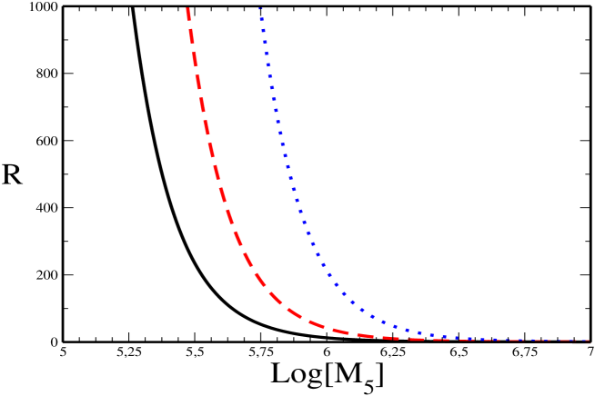
Figure 1: The enhancement/suppression factor $R=(\Omega_{\chi}h^{2})_{b}/(\Omega_{\chi}h^{2})_{s}$ as a function of the five dimensional scale $M_{5}$ (GeV) for $m_{\chi}=100$ (solid curve), $200$ (dashed curve) and $500$ GeV (dotted curve).

As advocated above, in brane cosmology the relic density $(\Omega_{\chi}h^{2})_{b}$ is quite sensitive to the value of the fundamental scale $M_{5}$ which should satisfy the upper bound given in Eq.(32). Therefore, with $m_{\chi}\simeq{\cal O}(100)$ GeV and $x_{F}\simeq{\cal O}(10)$, one finds

$$M_{5}<10^{7}.$$ (42)

Furthermore, the fact that the transition process from non-conventional cosmology to convention cosmology should take place above the nucleosynthesis era (i.e., $T_{t}>1$ MeV) impose the following lower bound on $M_{5}$:

$$M_{5}\raise 1.29167pt\hbox{$\;>$\kern-7.5pt\raise-4.73611pt\hbox{$\sim\;$}}1.2\times 10^{4}.$$ (43)

In Fig. 1, we present the prediction for the factor $R$ as a function of the scale of the five dimensions, $M_{5}$, for different values of $m_{\chi}$, namely we consider $m_{\chi}=100,200$ and $500$ GeV. As can be seen from this figure, for $M_{5}<10^{6}$ the brane cosmology effect is quite large and the factor $R$ becomes much larger than one. In this case the resulting relic density $(\Omega_{\chi}h^{2})_{b}$ may exceed the WMAP results (at $95\%$ confidence level) [3]

$$\Omega_{\chi}h^{2}=0.1126^{+0.0161}_{-0.0181}.$$ (44)

Moreover for $M_{5}\raise 1.29167pt\hbox{$\;>$\kern-7.5pt\raise-4.73611pt\hbox{$\sim\;$}}5\times 10^{6}$, the ratio $R$ becomes less than one and a small suppression for $(\Omega_{\chi}h^{2})_{s}$ can be obtained. This brane enhancement or suppression for the dark matter relic density could be favored or disfavored based on the value of the relic abundance in the standard scenario. If $(\Omega_{\chi}h^{2})_{s}$ is already larger than the observational limit, as in the case of bino-like particle, then a suppression effect would be favored and hence $M_{5}$ is constrained to be larger than $5\times 10^{6}$ GeV. However, for wino- or Higgsino-like particle where the standard computation usually leads to very small relic density, the enhancement effect will be favored and the constraint on $M_{5}$ can be relaxed a bit [5]. In general, it is remarkable that in this scenario the dark matter relic density imposes a stringent constraint on the fundamental scale $M_{5}$.

4 DM relic density in brane cosmology with low reheating temperature

In the standard computation for the DM relic density that we have adopted in the previous section, it was assumed that the reheating temperature $T_{RH}$ is much higher than the WIMP freeze-out temperature i.e., $T_{RH}\gg T_{F}$. In this case, the reheating epoch has no impact on the final result of the relic density. However, it is well known that the only constraint on $T_{RH}$ is $T_{RH}\raise 1.29167pt\hbox{$\;>$\kern-7.5pt\raise-4.73611pt\hbox{$\sim\;$}}1$ MeV in order not to spoil the successful predictions of the big bang neucleosynthesis. Therefore, in principle it is possible to have a cosmological scenario with low reheating such that $T_{RH}<T_{F}$. In this case the predictions of the relic abundance of the WIMP are modified as emphasized in Ref.[7] and recently in Ref.[8].

As in the previous section and to emphasize the effect of the brane cosmology, we assume that the WIMP freeze-out temperature is larger than the transition temperature which is also larger than the reheating temperature, i.e., $T_{F}>T_{t}>T_{RH}$. Within a low reheating temperature scenario, the relic density depends on whether WIMPs are never in chemical equilibrium either before or after reheating or they reach chemical equilibrium but they freeze-out before the completion of the reheat process. The resultant relic density in these two scenarios are quite different and are also different from the one derived by the standard computation with a large reheating temperature.

Let us start our analysis with the case of non-equilibrium production and freeze-out. In this case, at early times the number density $n_{\chi}$ is much smaller than $n_{\chi}^{eq}$ and the Boltzmann equation (28) can be written as

$$\frac{dY}{dx}=0.02095\left(\frac{g_{\chi}}{g_{*s}}\right)^{2}\frac{s}{Hx}\langle\sigma^{ann}_{\chi}\ v\rangle~{}x^{3}~{}e^{-2x}.$$ (45)

Although this equation is valid only at early times, it can be approximately integrated in the full range of $x$, namely from $x=0$ to $x=\infty$ due to the exponential suppression in the right hand side. Thus for the standard cosmology (where $H\propto x^{-2}$), one can easily integrate this equation and obtains

$$Y_{\infty s}=0.02095\sqrt{\frac{\pi}{45}}g_{\chi}^{2}g_{*}^{-3/2}M_{pl}~{}m_{\chi}\left(\frac{a}{4}+3b\right).$$ (46)

The $Y_{\infty}$ is related to the mass density of $\chi$ particle today as follows, at reheating we have $\rho_{\chi}(T_{RH})=m_{\chi}n_{\chi}(T_{RH})=\frac{2\pi^{2}}{45}g_{*s}(T_{RH})m_{\chi}Y_{\infty}T_{RH}^{3}$. After the reheating the universe is radiation dominated and the following relation is satisfied [7]:

$$\frac{\rho_{\chi}(T_{now})}{\rho_{R}(T_{now})}=\frac{T_{RH}}{T_{now}}~{}\frac{\rho_{\chi}(T_{RH})}{\rho_{R}(T_{RH})}.$$ (47)

Therefore, in this case $\Omega_{\chi}h^{2}$ is proportional to the annihilation cross section instead of being inversely proportional as in case of high reheating temperature.

Now we consider this scenario of low reheating with non-equilibrium production and freeze-out in brane cosmology. The Boltzmann equation is still given by Eq.(45), but with $H=(k_{2}x^{-4}+k_{3}x^{-8})^{1/2}$ in the range of $x\in[0,x_{t}]$ and with the usual Hubble parameter $H=\sqrt{k_{2}}x^{-2}$ between $x_{t}$ and $x=\infty$. Integrating this equation one finds

$$Y_{\infty b}\simeq 0.02095\times 10^{-6}\sqrt{\frac{\pi}{45}}g_{\chi}^{2}g_{*}^{-3/2}M_{pl}~{}m_{\chi}\left(9.46~{}a+37.8~{}b\right).$$ (48)

Here we have used $m_{\chi}\sim 100$ GeV and $M_{5}\sim 10^{6}$ GeV, as an example, to do the integration numerically. However, we have checked the result of $Y_{\infty b}$ for different values of $m_{\chi}$ and $M_{5}$. It turns out that $Y_{\infty b}$ is diminished significantly for $M_{5}\raise 1.29167pt\hbox{$\;<$\kern-7.5pt\raise-4.73611pt\hbox{$\sim\;$}}10^{6}$. As can be observed from equations (46) and (48) that this non-equilibrium scenario produces a very suppressed relic density, particularly in brane cosmology. Furthermore, the assumption that $n_{\chi}\ll n_{\chi}^{eq}$ impose a sever constraint on the annihilation cross section. Thus, one can conclude that within this scenario, it is not possible to account for the dark matter experimental results.

Now we turn to the second scenario in which the annihilation cross section of the WIMP is large and hence it reaches the chemical equilibrium before reheating. In this case, the computation of the relic density $\Omega_{\chi}h^{2}$ is very close to the standard case with high reheating temperature. At the early times i.e., when $T>T_{F}$, the WIMP’s are very close to equilibrium. So, as usual, one can use the variable $\Delta(x)=Y(x)-Y^{eq}(x)$ to write the Boltzmann equation as

$$\Delta^{\prime}=-(Y^{eq})^{{}^{\prime}}-f(x)\Delta\left(2Y^{eq}+\Delta\right),$$ (49)

where $f(x)$ is given by $f(x)=\sqrt{\frac{\pi g_{*}}{45}}M_{pl}m_{\chi}\left[\frac{a}{x^{2}}+\frac{6b}{x^{3}}\right].$ Then by neglecting $\Delta^{\prime}$ and $\Delta^{2}$ , one obtains

$$\Delta\simeq-\frac{(Y^{eq})^{{}^{\prime}}}{2f(x)Y^{eq}}.$$ (50)

At late time, when $T<T_{F}$ one gets $Y\gg Y^{eq}$ and hence we can use the approximation $Y^{2}-(Y^{eq})^{2}\simeq Y^{2}$ in Eq.(29) and integrate from $T_{F}$ down to $T_{RH}$ to determine $Y(T_{RH})$. In the standard cosmology, one finds

$$\frac{1}{Y(x_{RH})}\Big{|}_{s}=\frac{1}{Y(x_{F})}-\sqrt{\frac{\pi g_{*}}{45}}M_{pl}m_{\chi}\left[\frac{a}{x}+\frac{3b}{x^{2}}\right]_{x_{F}}^{x_{RH}},$$ (51)

If it is assumed that there is no entropy production for $T<T_{RH}$, then there is no WIMP production for temperature below the reheating temperature. Thus, the present value of $Y$ is given by $Y(x_{RH})$ up to an overall correction due to the fact that the reheating process is not complete at $T_{RH}$ [7]. Here, two comments are in order: $i)$ As mentioned above, $Y(x_{F})^{-1}\simeq Y_{eq}(x_{F})^{-1}$ which is of order ${\cal O}(10^{9})$, so its contribution to $Y(x_{RH})^{-1}$ in Eq.(51) can be neglected respected to the second term. $ii)$ Since $T_{RH}<T_{F}$ (i.e., $x_{RH}>x_{F}$), one can approximate Eq.(51) and finds that the relic abundance $\Omega_{\chi}h^{2}$ is very close to the one obtained by using the standard calculation with high reheating temperature, namely

$$\Omega_{\chi}h^{2}\sim 1.1\times 10^{-11}\left(\frac{a}{x_{F}}+\frac{3b}{x_{F}^{2}}\right)^{-1},$$ (52)

which implies that unless annihilation cross sections are quite small ($\raise 1.29167pt\hbox{$\;<$\kern-7.5pt\raise-4.73611pt\hbox{$\sim\;$}}10^{-8}$), one gets, as usual, very small relic density.

In brane cosmology, Eq.(30) describes the correct Boltzmann equation that should be used. Also, as in the previous scenario, one has to integrate this equation from $x_{F}$ to $x_{t}$ using brane cosmology feature, and from $x_{t}$ to $x_{RH}$ using the standard cosmology feature. In this respect, one finds

$$\frac{1}{Y(x_{RH})}\Big{|}_{b} = \frac{1}{Y(x_{F})}-\sqrt{\frac{\pi g_{\ast}}{45}}M_{pl}m_{\chi}\left[3\sqrt{\frac{k_{2}}{k_{3}}}b\left(\sinh^{-1}\left(\sqrt{\frac{k_{3}}{k_{2}}}x_{F}^{-2}\right)-\sinh^{-1}\left(\sqrt{\frac{k_{3}}{k_{2}}}x_{t}^{-2}\right)\right)\right.$$ (53)

$$+ \left.a\left(\frac{1}{x}~{}_{2}F_{1}\left[\frac{1}{4},\frac{1}{2},\frac{5}{4},\frac{-k_{3}}{k_{2}x^{4}}\right]\right)^{x_{t}}_{x_{F}}+\left(\frac{a}{x}+\frac{3b}{x^{2}}\right)^{x_{RH}}_{x_{t}}\right].$$

One can easily check that the three parts of the second term in the above equation are of the same order and give the dominant contribution to $Y(x_{RH})^{-1}$. In this case, one can show that the relic density (for $m_{\chi}=100$ GeV and $M_{5}=10^{6}$ GeV) is given by

$$\Omega_{\chi}h^{2}\sim 1.1\times 10^{-7}\left(95.2~{}a-4.12~{}b\right)^{-1}.$$ (54)

From this equation it can be easily seen that even with large annihilation cross section ${\cal O}(10^{-6}-10^{-8})$, we are able to obtain the cosmologically interesting value $\Omega_{\chi}h^{2}\sim 0.1$. This implies that the scenario of brane cosmology with low reheating termperature and chemical equilibrium WIMPs is the most interesting model for dark matter. It provide an interesting possibility for having dark matter with large cross section (hence their detection would be possible in future DM experiments) with suitable relic aboundanc.

5 Conclusions

In this paper we have analyzed the relic abundance of cold dark matter in brane cosmology. We have pointed out that the consistency of the boundary conditions that account for the presence of the brane implies that the $5D$ metric should contain, at least, two warp factors. In case of one warp factor, we have emphasized that the relation $\rho_{b}=-p_{b}$ is identically satisfied, which contradicts the possibility of having matter on the brane.

We have also studied the impact of brane cosmology on the cold dark matter relic density. We investigated this effect in two different scenarios, namely when the reheating temperature is higher or lower than the freeze-out temperature. We showed that with high reheating temperature, the relic density is enhanced with many order of magnitude for $M_{5}\raise 1.29167pt\hbox{$\;<$\kern-7.5pt\raise-4.73611pt\hbox{$\sim\;$}}10^{6}$. This imposes one of the strongest constraints on the scale of large extra dimensions. In case of low reheating temperature, we have considered the possibility that WIMPs are in chemical equilibrium or non-equilibrium, which depends on the value of their annihilation cross section. We emphasized that if WIMPs are in chemical non-equilibrium, then their relic density is very small and they can not account for the observational limits. While in case WIMPs reach chemical equilibrium before reheating, we showed that the relic density is enhanced by two order of magnitudes than the standard thermal scenario result. This enhancement can be considered as an interesting possibility for accommodating dark matter with large cross section, which is favored by the detection rate experiments.

References

- [1] L. Randall and R. Sundrum, Phys. Rev. Lett. 83, 3370 (1999); L. Randall and R. Sundrum, Phys. Rev. Lett. 83, 4690 (1999).
- [2] P. Binetruy, C. Deffayet and D. Langlois, Nucl. Phys. B 565, 269 (2000);P. Binetruy, C. Deffayet, U. Ellwanger and D. Langlois, Phys. Lett. B 477, 285 (2000); D. Langlois, Prog. Theor. Phys. Suppl. 148, 181 (2003); E. E. Flanagan, S. H. H. Tye and I. Wasserman, Phys. Rev. D 62, 044039 (2000); P. Kanti, I. I. Kogan, K. A. Olive and M. Pospelov, Phys. Lett. B 468, 31 (1999); J. M. Cline, C. Grojean and G. Servant, Phys. Rev. Lett. 83, 4245 (1999);C. Csaki, M. Graesser, C. F. Kolda and J. Terning, Phys. Lett. B 462, 34 (1999); C. Csaki, M. Graesser, L. Randall and J. Terning, Phys. Rev. D 62, 045015 (2000)
-
[3]
C. L. Bennett et al., Astrophys. J. Suppl. 148, 1 (2003);
D. N. Spergel et al. [WMAP Collaboration], Astrophys. J. Suppl. 148, 175 (2003). - [4] N. Okada and O. Seto, Phys. Rev. D 70, 083531 (2004); T. Nihei, N. Okada and O. Seto, Phys. Rev. D 71, 063535 (2005).
- [5] T. Nihei, N. Okada and O. Seto, Phys. Rev. D 73, 063518 (2006).
- [6] M. Arik and D. Ciftci, Gen. Rel. Grav. 37, 2211 (2005) [arXiv:gr-qc/0506094].
- [7] G. F. Giudice, E. W. Kolb and A. Riotto, Phys. Rev. D 64, 023508 (2001)
- [8] S. Khalil, C. Munoz and E. Torrente-Lujan, New J. Phys. 4 (2002) 27; C. Pallis, Astropart. Phys. 21 (2004) 689; G. B. Gelmini and P. Gondolo, arXiv:hep-ph/0602230; G. Gelmini, P. Gondolo, A. Soldatenko and C. E. Yaguna, arXiv:hep-ph/0605016; M. Endo and F. Takahashi, arXiv:hep-ph/0606075.