Juan Rojo Chacón     Julio 2006 5 José Ignacio Latorre Sentís - Universitat de Barcelona
Dr. Stefano Forte - Università di Milano Estructura i Constituents de la Matèria Programa de Doctorado: Física Avanzada
Bienio: 2002-2004

THE NEURAL NETWORK APPROACH TO PARTON DISTRIBUTIONS

A Sònia

Agradecimentos

La realización de una tesis doctoral, más que una obra individual, es por encima de todo una tarea comunitaria. Por esto los agradecimientos son el momento en el cual se tienen en cuenta la contribución de todas aquellas personas que con sus aportaciones de todo tipo han permitido que la presente tesis doctoral haya llegado a buen puerto.

En primer lugar quisiera agradecer a José Ignacio Latorre por acompañarme estos cuatro años como director de esta tesis doctoral. Desde sus primeras clases de Física de Altas Energías, me cautivó la pasión con la que explicaba, que es la misma con la que vive la aventura de la investigación científica. José Ignacio ha sido para mí no solo un maestro en el campo de la ciencia sino también un modelo por su honestidad en todos los ámbitos.

También aprovecho para agradecer al codirector de esta tesis doctoral, Stefano Forte. Con Stefano he aprendido el rigor necesario para ser un buen científico, así como la pasión necesaria para afrontar incluso los problemas más difíciles sin desfallecer. Su ayuda continua han sido esenciales para llevar a cabo el trabajo de investigación desarrollado en esta tesis doctoral.

Muchas han sido las personas con las cuales durante estos cuatro años he compartido el placer de la investigación científica, aprendiendo continuamente de todos ellos. De manera especial a los otros miembros de la NNPDF Collaboration, Andrea Piccione y Luigi Del Debbio, pero también a muchas otras personas: Antonio Pineda, Jorge Russo, Giovanni Ridolfi, Concha Gonzalez-García, Michele Maltoni… Asimismo, querriá agradecer a todas aquellas personas con las que he compartido siempre instructivas discusiones sobre física, y con las cuales he aprendido poco a poco el arte de ser investigador. La lista es muy larga: Germán Rodrigo, Joan Soto, Ignazio Scimemi, Thomas Becher, Einan Gardi …

También querría agradecer a todos aquellos compañeros del departamento de Estructura i Contituents de la Matèria con los que he pasado estos años, compartiendo la aventura de realizar una tesis doctoral: Xavi, Enrique, Román, Diego, Dani, Míriam, Luca, Jaume, Alex … Pero especialmente a Manel y Arnau, pues desde que nos conocimos en el primer curso de la licenciatura, nos hemos acompañado a lo largo de toda la carrera y el doctorado. Parece que aquel dia tan lejano que apenas dislumbrabamos cuando hacíamos Fonaments de Física ahora está cerca para los tres. También estoy agradecido a Joan Soto y Nuria Barberán por comunicarme tanto su pasión como su rigor en la docencia de las asignaturas que yo he colaborado a impartir en los dos últimos años. Finalmente, agradecer a Oriol y a Rosa su continua ayuda en tantos detalles prácticos que han surgido en estos años.

Son tantos los amigos que a lo largo de estos cuatro años me han acompañado en la apasionante aventura de la vida, haciendo posible renovar continuamente la pasión por todo, incluyendo la investigación científica, que pido perdón por adelantado por todos aquellos que no tengo presentes. A Juan Ramón y a Roger especialmente por su inasequible apoyo y su continua ayuda en el cuidar la no siempre fácil vocación científica. A Lluís por comunicarme su pasión por el conocimiento y por la vida, y por proponerme una amistad que dura hasta hoy. A todos aquellos amigos que hemos vivido juntos estos años: Néstor, Raquel, Jorge, Xavi, Alfonso, Anna, Miquel C., Cristina, Miquel, Josep C., Josep M., Marc, Albert …, gracias una vez más por vuestra infatigable compañia en este camino.

También estoy profundamente agradecido a los amigos de física de Milán: Giuliano, Tommy, Betta, Paola, Maria, y a toda la asociación cultural Euresis, por ayudarme a vivir mi vocación científica con un horizonte abierto a toda la realidad. También aprovecho para agradecer a los amigos de Madrid de la Asociación Universitas, por su empeño continuo en vivir la vida académica siempre consciente de las razones de la propia vocación, y por tanto posibilitando renovar siempre el interés tanto por la docencia como por la investigación.

Sin embargo, por encima de todo quería agradecer a mi familia todo el apoyo y la ayuda incansable que me han proporcionado a lo largo todos estos años. Mi padre Eduardo ha sido desde siempre mi referencia, tanto a nivel académico como a nivel personal. La pasión y la alegría con la que mi padre vive su trabajo en la Universidad han sido mi mayor motivación para empezar física primero, y decidirme por la carrera académica después. Mi madre Carmen también me ha ayudado siempre a valorar el estudio y el trabajo, educandome en el interés por toda la realidad, algo que nunca podré agradecer suficientemente. Mi hermano Ignacio ha sido siempre modelo para mí, por la pasión y seriedad con la que ha vivido siempre el estudio, y ahora el trabajo. También estoy muy agradecido a mi familia política, Raül, Margarita, Olga y Montserrat, por su continuo apoyo a todos los niveles en la realización de esta tesis doctoral.

Finalmente, todo mi agradecimiento va dirigido a mi mujer, Sònia. Gracias a ella, a su ayuda y su estímulo, he podido realizar la presente tesis doctoral. Su apoyo infatigable en todas las circunstancias ha sido lo que me ha permitido empezar cada día con una ilusión plenamente renovada, tanto en la investigación como en la docencia. Por todo ello, no puedo más que agradecerle otra vez todos estos años en que nos hemos acompañado en la apasionante aventura de la vida y el matrimonio.

Research articles - published

• J. Rojo and J. I. Latorre [condensates], “Neural network parametrization of spectral functions from hadronic tau decays and determination of QCD vacuum condensates,” JHEP 0401, 055 (2004) [arXiv:hep-ph/0401047].

• J. Brugues, J. Rojo and J. G. Russo [strings], “Non-perturbative states in type II superstring theory from classical spinning membranes,” Nucl. Phys. B 710, 117 (2005), [arXiv:hep-th/0408174].

• L. Del Debbio, S. Forte, J. I. Latorre, A. Piccione and J. Rojo [f2nnp], “Unbiased determination of the proton structure function $F_{2}^{p}$ with faithful uncertainty estimation”, JHEP 0503 (2005) 080, [arXiv:hep-ph/0501067].

• S. Forte, G. Ridolfi, J. Rojo and M. Ubiali [landau], “Borel resummation of soft gluon radiation and higher twists,” arXiv:hep-ph/0601048, Phys. Lett. B 635 (2006) 313.

• J. Rojo [bmeson], “Neural network parametrization of the lepton energy spectrum in B meson decays”, JHEP 0605 (2006) 040 [arXiv:hep-ph/0601229].

• J. Mondejar, A. Pineda and J. Rojo [rojoscet], “Heavy meson semileptonic differential decay rate in two dimensions in the large $N_{c}$,” arXiv:hep-ph/0605248.

Research articles - in preparation

• L. Del Debbio, S. Forte, J. I. Latorre, A. Piccione and J. Rojo [NNPDF Collaboration], “The neural network approach to parton distributions: The nonsinglet case”, UB-ECM-PF 06/17.

• C. García-González, M. Maltoni and J. Rojo, “Neural network parametrization of the atmospheric neutrino flux”, in preparation.

• L. Del Debbio, S. Forte, J. I. Latorre, A. Piccione and J. Rojo [NNPDF Collaboration], “The neural network approach to parton distributions: The singlet case”, in preparation.

Conference proceedings

• J. Rojo, “A probability measure in the space of spectral functions and structure functions” [proc1], proceedings of the QCD International Conference, Montpellier 2004, Nucl. Phys. B (Proc. Suppl.) 152 (2006) 57, arXiv:hep-ph/0407147.

• J. Rojo, L. Del Debbio, S. Forte, J. I. Latorre and A. Piccione [NNPDF Collaboration] [proc2], “The neural network approach to parton fitting,” proceedings of DIS05 workshop, arXiv:hep-ph/0505044.

• J. Rojo, L. Del Debbio, S. Forte, J. I. Latorre and A. Piccione [NNPDF Collaboration] [proc3], “The neural network approach to parton distributions,” contribution to the proceedings of the Hera-LHC workshop, hep-ph/0509059.

• J. Rojo, L. Del Debbio, S. Forte, J. I. Latorre and A. Piccione [NNPDF Collaboration] [procacat], “The neural network approach to parton fitting,” proceedings of the ACAT05 workshop, hep-ph/0509067.

Chapter 1 Introducción

El Large Hadron Collider (LHC, gran colisionador de hadrones) es un colisionador de protones a las energías más elevadas conseguidas artificialmente por el hombre, situado en el Centro Europeo para la Investigación Nuclear, el CERN en Ginebra (Suiza). Este acelerador de partículas está actualmente en construcción, y se espera que las primeras colisiones de protones se produzcan antes del final del año 2007. Las enormes energías que se alcanzarán en las colisiones entre protones en el LHC nos permitirán examinar las leyes fundamentales de la naturaleza a las menores distancias jamás investigadas. En particular, se estudiará en detalle el mecanismo de la ruptura de simetría electrodébil, mediada por la partícula de Higgs, que es la responsable de dar las masas a todas las partículas elementales conocidas. Además, se espera que LHC nos proporcione información detallada sobre nueva física mas allá del Modelo Estandard de Física de Partículas, que ha sido construido y comprobado con enorme éxito durante los ultimos 25 años. En la fig. 1.1 podemos ver la localización del experimento LHC cerca de Ginebra, así como uno de sus detectores, ATLAS, donde se examinan los resultados de la colisiones entre protones.

Figure 1.1:

La localización del túnel de 27 kilómetros donde está situado el LHC, cerca de Ginebra (los Alpes pueden ser vislumbrados detrás) (izquierda) y uno de sus detectores, ATLAS, que es tan grande como un edificio de siete pisos (derecha).

Sin embargo, la extracción de la nueva física de las colisiones protón-protón a altas energías que se producirán en el LHC es una tarea extremadamente complicada, por una serie de motivos que detallaremos a continuación. El principal de estos motivos es que esta nueva física estará escondida entre una multitud de procesos de física conocida, debido a la interacción fuerte entre quarks y gluones (que son las partículas elementales que componen los protones) determinadas por el Modelo Estandard, en particular por la teoría conocida como Cromodinámica Cuántica (Quantum Chromodynamics, QCD). Estos procesos serán mucho más frecuentes que las colisiones en donde se produzcan los efectos buscados de nueva física. Por lo tanto, el potencial de descubrimiento del LHC, así como su habilidad para realizar medidas de precisión de las propiedades de esta nueva física, dependen de una manera crucial de nuestra comprensión quantitativa de los procesos de la interacción fuerte y las incertidumbres que estos llevan asociados. En la fig. 1.2 podemos ver el resultado de un proceso característico de colisión entre protones en el LHC. Es necesario recalcar que de los miles de millones de colisiones como esta que se producirán cada año en el LHC, será necesario extraer aquellas pocas que contienen información auténticamente relevante.

Figure 1.2:

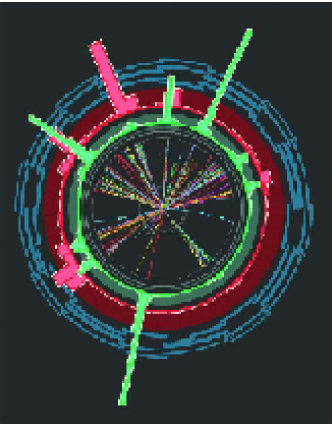
Resultado de una colisión típica entre protones en el LHC: podemos observar las trazas que dejan los cientos de partículas producidas en cada colisión, así como la energía total que cada una de estas partículas lleva asociada.

Entre las diversas fuentes de incertidumbre asociadas a los procesos que involucran partículas con interacción fuerte, una de las de mayor importancia es debida a las distribuciones de partones (Parton Distribution Functions, PDFs) en el interior del protón. Estas distribuciones son una medida de la cantidad de la energía total del protón que lleva cada uno de sus diversos componentes, los quarks de diferente sabor y los gluones. Estas distribuciones de partones no pueden ser calculadas en teoría de perturbaciones, sino que necesitan ser extraidas de los datos experimentales que provienen de una gran cantidad de procesos de física de altas energías, como por ejemplo las colisiones profundamente inelásticas (Deep inelastic scattering, DIS) entre leptones (partículas elementales sin interacción fuerte) y protones.

Las distribuciones de partones las denotaremos por

$$q_{i}(x,Q^{2})\ ,\quad i=1,\ldots,2N_{f}+1\ ,$$ (1.1)

donde $Q^{2}$ es la energia típica del proceso de colisión, la variable $x$ denota la fracción de la energía total del protón que lleva el parton $i$, y tenemos una distribución de partones independiente para cada quark y cada antiquark de diferente sabor, más una para los gluones. Hay que tener en cuenta que en QCD las energías son grandes o pequeñas en comparación con la masa del proton $M_{p}$, que constituye la escala característica de la teoría. Estas distribuciones de partones pueden ser determinadas gracias a la existencia del teorema conocido como el Teorema de la Factorización en Cromodinámica Cuántica. Segun este teorema, cualquier sección eficaz de colisión (que mide la probabilidad de que dos partículas colisionen y interaccionen) en procesos que involucren la interación fuerte puede ser separada en el producto de dos términos: un coeficiente que depende del proceso en cuestión, que podemos calcular en teoría de perturbaciones, y un conjunto de distribuciones de partones que son universales, es decir, que son independientes de los detalles particulares del proceso. En la fig. 1.3 observamos un esquema del interior de un protón, con los diferentes quarks interaccionando entre si mediante los gluones, y donde la flecha indica el spin, el momento angular interno de cada partícula. El movimiento de estos quarks y gluones en el protón viene dictado por estas distribuciones de partones.

Figure 1.3:

El interior de un protón se compone de quarks y antiquarks de diferentes sabores, junto con gluones que mediante la interacción fuerte mantienen a estos quarks confinados en el interior del protón.

Por ejemplo, las funciones de estructura en colisiones profundamente inelásticas pueden escribirse como

$$F(x,Q^{2})=C_{i}\left(x,\alpha_{s}\left(Q^{2}\right)\right)\otimes q_{i}(x,Q^{2})\ ,$$ (1.2)

es decir, como la convolución entre un coeficiente $C_{i}(x)$ que depende del proceso y las distribuciones de partones $q_{i}(x)$, que son idénticas para todo proceso de colisión a altas energías que involucre partículas con la interacción fuerte en el estado inicial. Solamente es necesario determinar las distribuciones de partones a una escala inicial $Q^{2}_{0}$ relativamente pequeña, $Q^{2}_{0}\sim M_{p}^{2}$, pues su dependencia con la energía (denominada evolución) viene dictada por la teoría de perturbaciones de la Cromodinámica Cuántica. Es necesario tener en cuenta que en general diferentes combinaciones de distribuciones de partones contribuyen a cada observable de manera diferente. Aunque la mayor fuente de información experimental sobre las distribuciones de partones proviene de las medidas de alta precisión en los procesos de colisión profundamente inelásticos descritos anteriormente, otros procesos son esenciales como producción de jets (conjuntos de hadrones, es decir, de partículas que interaccionan fuertemente) en colisiones de protones o el proceso de Drell-Yan, esto es, la producción de parejas de leptones también en colisiones entre hadrones.

El requisito de poder realizar física de precisión en colisionadores de protones, como el futuro LHC, implica que es necesario determinar con la mayor exactitud posible no solamente las diferentes distribuciones de partones en el protón, $q_{i}(x,Q_{0}^{2})$, sino también las incertidumbres que estas tienen asociadas. Estas incertidumbres provienen del hecho de que puesto que las distribuciones de partones se extraen de datos experimentales, que tienen una precisión finita, también estas tendrán a su vez una precisión finita, es decir, un error experimental asociado. Para ver la importancia capital que las distribuciones de partones tendrán en el LHC, es necesario notar que una sección eficaz de colisión típica tiene la forma

$$\sigma(x,Q^{2})=C_{ij}\left(x,\alpha_{s}\left(Q^{2}\right)\right)\otimes q_{i}(x,Q^{2})\otimes q_{j}(x,Q^{2})\ ,$$ (1.3)

es decir, que depende de dos distribuciones de partones, una para cada de los partones que involucran las colisiones protón-protón. Este problema es particularmente grave pues la region cinemática que cubrirá el LHC ha sido solamente parcialmente cubierta por aquellos experimentos que han sido usados para determinar las distribuciones de partones con anterioridad, como HERA y SLAC (ver fig. 1.4), y por lo tanto será necesario extrapolar las distribuciones de partones a regiones donde nunca han sido medidas. Es importante, por lo tanto, controlar de manera muy precisa las incertidumbres asociadas a este proceso de extrapolación.

Figure 1.4:

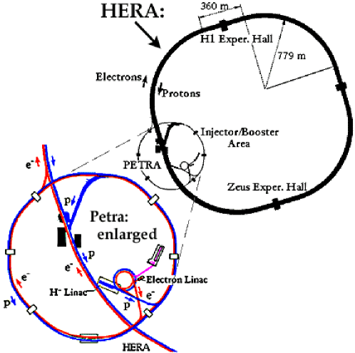
Esquema del experimento de colisiones profundamente inelásticas HERA en Hamburgo.

El problema principal, en vista de todo lo descrito anteriormente, es determinar los errores de una función continua como son las distribuciones de partones, es decir, una densidad de probabilidad en el espacio de estas funciones, a partir de un conjunto finito de datos experimentales. Existe toda una serie de técnicas estandard para determinar las distribuciones de partones a partir de las medidas experimentales, y diversas estrategias han sido usadas para estimar de maneras diversas además los errores asociados a estas distribuciones. Todas estas estrategias han sido útiles para estimar de manera aproximada el tamaño de estas incertidumbres, pero sin embargo sufren de un cierto número de problemas. Con las técnicas estandard, las distribuciones de partones se parametrizan con funciones relativamente simples, típicamente polinomios de la forma

$$q_{i}(x,Q^{2}_{0})=A_{i}x^{b_{i}}\left(1-x\right)^{c_{i}}\left(1+d_{i}x+e_{i}x^{2}\right)\ ,\qquad i=1,\ldots,N_{f}+1\ ,$$ (1.4)

donde los parametros $A_{i},b_{i}\ldots$ se determinan a partir de un fit de los datos experimentales. El primer problema aparece de immediato: nos estamos restringiendo al espacio de distribuciones de partones parametrizadas por la ec. 1.4, lo cual está claramente injustificado pues no hay en la Cromodinámica Cuántica, la teoría que en principio determina la forma de estas distribuciones, nada que implique que las distribuciones de partones han de tener la forma funcional tan específica que podemos observar en la ec. 1.4. Segundo, si se quieren propagar los errores que la ec. 1.4 lleva asociados a otros observables, como secciones eficaces de la forma de la ec 1.3, son necesarias aproximaciones de linealización, que como es bien conocido no son válidas en un amplio rango de situaciones. Finalmente, el tercer inconveniente que presenta la técnica estandard es que en presencia de datos experimentales que provienen de experimentos diferentes, la presencia de incompatibilidades entre los datos (por ejemplo, que la función de estructura, ec. 1.2, medida en dos experimentos distintos sea muy diferente) implica que la condición para determinar los errores a partir de la función de error $\chi^{2}$ no es $\Delta\chi^{2}=1$, como indica la estadística básica, sino $\Delta\chi^{2}=100$. En la práctica esta elección implica que los errores de las distribuciones de partones no tienen ningún significado estadístico riguroso pues dependen de un parámetro arbitrario $\Delta\chi^{2}$. En la fig. 1.5 tenemos un ejemplo de una determinación reciente de distribuciones de partones junto con las incertidumbres asociadas. Notemos que hay dos tipos de errores asociados: los errores estadísticos habituales (debido a disponer de un número finito de medidas) y los errores sistemáticos, que dependen en general del proceso de medida y que están correlacionados entre diferentes datos experimentales.

Figure 1.5:

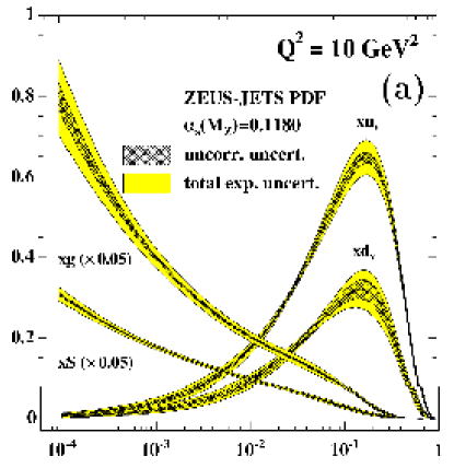
Un ejemplo de una determinación reciente de distribuciones de partones. Notemos que cada distribución tiene asociada una banda de incertidumbre, que es una medida de los errores de cada una de las distribuciones de partones.

Por todas las razones descritas hasta ahora, y en vista de la importancia crucial que una estimación fidedigna de las incertidumbres asociadas a las distribuciones de partones tiene para la física de precisión en el LHC, es claramente deseable investigar estrategias alternativas para la determinación de estas distribuciones que permitan superar y mejorar los problemas de la técnica estandard descrita anteriormente. En [f2ns] una novedosa técnica fue presentada consistente en la determinación de la densidad de probabilidad en el espacio de las funciones, que fue aplicada a la parametrización de funciones de estructura, como la ec. 1.2, en procesos de colisión profundamente inelásticos entre leptones y protones. Esta novedosa técnica usaba una combinación de métodos Monte Carlo para la construcción de samplings de los datos experimentales junto con redes neuronales artificiales como interpolantes universales. El uso de redes neuronales artificiales en lugar de funciones polinómicas como la eq. 1.4 en la parametrización de las distribuciones de partones permite eliminar la dependencia de los resultados en la forma funcional escogida arbitrariamente. Por su parte, la técnica de los samplings Monte Carlo permite una estimación estadísticamente rigurosa de las incertidumbres asociadas a la función que estamos parametrizando, y además la propagación de estos errores a otros observables se puede realizar con toda generalidad, sin necesidad de aproximaciones de linearización.

En la presente tesis doctoral hemos extendido los resultados presentados en [f2ns], aplicados a las funciones de estructura en colisiones profundamente inelásticas, en diversas direcciones. En primer lugar hemos aplicado esta técnica general para parametrizar datos experimentales a otros procesos de interés en física de altas energías. Los procesos que han sido estudiados son las desintegraciones hadrónicas del lepton tau, las desintegraciones semileptónicas del mesón B, y las colisiones profundamente inelásticas desde dos puntos de vista: a nivel de funciones de estructura, incluyendo todos los datos experimentales a nuestra disposición, y a nivel de distribuciones de partones non-singlet, es decir, cuando el gluon se ha desacoplado del resto de distribuciones. En cada una de estas aplicaciones, la relación entre los datos experimentales y la función a parametrizar era diferente, demostrando que la técnica descrita en esta tesis es completamente general, válida para un gran número de situaciones.

Además, en la presente tesis hemos extendido la estrategia original descrita en [f2ns] mediante la introducción de nuevos algoritmos para entrenar las redes neuronales artificiales, en particular los conocidos como Algoritmos Genéticos. Estos algoritmos son necesarios para entrenar redes neuronales mediante funciones de error altamente no lineales, como nos sucede en las diferentes aplicaciones que describiremos en esta tesis. Finalmente, se han mejorado las técnicas estadísticas utilizadas para la validación de los resultados obtenidos, esto es, de la densidad de probabilidad contruida en los diferentes casos. En el siguiente Capítulo describimos con cierto detalle los contenidos de la presente tesis doctoral y los resultados que han sido obtenidos.

Chapter 2 Resumen

La presente tesis doctoral está organizada de la manera que se describe con cierto detalle a continuación. En el Capítulo 4 hacemos un resumen de los elementos básicos de la Cromodinámica Cuántica, que como hemos explicado con anterioridad es el sector del Modelo Estandard de física de partículas que gobierna la llamada interacción fuerte entre partículas elementales. Asimismo, describimos también aquellos procesos de física de altas energías en los cuales utilizaremos la estrategia general para parametrizar datos experimental que constituye el principal objeto de esta tesis. Junto con este resumen, presentamos también una descripción detallada de la técnica estandard, discutida en el Capítulo anterior, que se usa comúnmente para extraer las distribuciones de partones con sus errores asociados a partir de un conjunto de datos experimentales.

A continuación, en el Capítulo 5 describimos con todo lujo de detalles la técnica general para construir la densidad de probabilidad de una función a partir de medidas experimentales, esto es, una técnica para parametrizar datos experimentales, sin necesidad de hacer hipótesis alguna sobre la forma funcional de la función a parametrizar y con una estimación fidedigna de las incertidumbres asociadas, que permite una propagación de los errores a observables arbitrarios sin necesidad de aproximaciones lineales. Este Capítulo está divido en tres partes, métodos Monte Carlo, redes neuronales artificiales y estimadores estadísticos, que procedemos a describir a continuación.

En la primera parte de este Capítulo se describen los métodos Monte Carlo que usamos para construir un sampling de los datos experimentales que contenga toda la información que nos proporcionan los experimentos, incluyendo los errores y las correlaciones. Asimismo, introducimos un conjunto de estimadores estadísticos que nos permiten estimar quantitativamente como este sampling Monte Carlo reproduce las características de las medidas experimentales. Esta técnica nos permite estimar de una manera fidedigna los errores asociados a la función a parametrizar, y demostraremos que es equivalente a los errores definidos a partir de una función de error $\chi^{2}$ cuando las aproximación lineales en la propagación de los errores son suficientes.

En la segunda parte del Capítulo 5 introducimos las redes neuronales artificiales, que utilizaremos como interpoladores universales, así como los diferentes métodos que usaremos para entrenar estas redes neuronales, esto es, para que aprendan los patterns presentes en los datos experimentales. Las redes neuronales artificiales son una herramienta habitual en diversos campos científicos, desde la biología a la computación, y en particular se usan con asiduidad en física experimental de altas energías, en aplicaciones como clasificación de eventos en función de sus propiedades. En la fig. 2.1 mostramos una red neuronal artificial de la clase que utilizaremos en esta tesis doctoral, conocida como multi-layer feed-forward perceptron. Asimismo describiremos como nuestra técnica permite la incorporación de información teórica de maneras muy diversas, como reglas de suma o condiciones implicadas por la cinemática del proceso.

Figure 2.1:

Diagrama esquemático de una red neuronal artificial multicapa del tipo feed-forward.

Las redes neuronales artificiales tienen la interesante propiedad de que es es posible demostrar que cualquier función continua, independientemente de lo complicada que sea y del número de parámetros que tenga, puede ser representada en términos de una multi-layer feed-forward red neuronal artificial. Una segunda propiedad importante de las redes neuronales artificiales es que estas son muy eficientes en combinar de una manera óptima la información experimental que proviene de diferentes medidas de una misma cantidad. Esto es, cuando la separación entre datos experimentales en el espacio de variables de entrada es más pequeña que una determinada longitud de correlación, entonces la red neuronal combina de manera eficiente esta información experimental, de manera que el correspondiente pattern de salida es mas preciso que las medidas experimentales individuales.

La utilidad de las redes neuronales artificiales es debida a la existencia de diversos algoritmos de entrenamiento. Este proceso se llama aprendizaje, pues no requiere un conocimiento a priori de la forma funcional que describe los datos experimentales. En particular, en la presente tesis doctoral hemos introducido los llamados algoritmos genéticos para el entrenamiento de redes neuronales artificiales. Estos algoritmos genéticos tienen un gran número de ventajas respecto a los métodos de minimización deterministas que los hacen preferibles para problemas, como los que nos ocupan en la presente tesis doctoral, altamente no lineales y con un enorme espacio de parámetros.

Las ventajas de los algoritmos genéticos, que como su propio nombre indica están inspirados en los mecanismos que se observan en la naturaleza sobre la evolución y la selección natural, se pueden resumir en tres. Primero de todo, estos algoritmos trabajan simultáneamente en poblaciones de soluciones, lo que les permite explorar regiones diferentes del espacio de parámetros al mismo tiempo. Segundo, no necesitan ninguna información extra de la función a minimizar, como el gradiente de esta. Finalmente, estos algoritmos tienen una mezcla de elementos estocásticos aplicados bajo reglas deterministas, que mejora su eficiencia en problemas con muchos extremos locales, pero sin la pérdida de efectividad que una búsqueda meramente aleatoria implicaría.

Finalmente, en la tercera parte del Capítulo, analizaremos aquellas herramientas estadísticas que nos permiten validar el resultado obtenido, esto es, determinar de una manera quantitativa como la densidad de probabilidad que hemos construido reproduce las caraterísticas de los datos experimentales, así como su dependencia con respecto diversos parámetros, como por ejemplo el número de redes neuronales empleadas en la parametrización. Estas técnicas estadísticas permiten también detereminar a partir de criterios sólidos características de la densidad de probabilidad como la longitud del entrenamiento de las redes neuronales o el valor óptimo de la función de error $\chi^{2}$.

El conjunto de redes neuronales artificiales entrenadas en el conjunto de replicas Monte Carlo de los datos experimentales para una función $F$ definen la densidad de probabilidad en el espacio de funciones $F$ que estábamos buscando. Con esta densidad de probabilidad, podemos obtener los valores esperados para funcionales arbitrarios de la función $F$, $\mathcal{F}\left[F\right]$, a partir del conjunto de redes neuronales de la manera siguiente,

$$\left\langle\mathcal{F}[F]\right\rangle\equiv\int\mathcal{D}F~{}\mathcal{P}\left[F\right]\mathcal{F}[F]=\frac{1}{N_{\mathrm{rep}}}\sum_{k=1}^{N_{\mathrm{rep}}}\mathcal{F}[F^{(\mathrm{net})(k)}]\ ,$$ (2.1)

como con las distribuciones de probabilidad habituales. De esta manera podemos determinar la media de $F$, su variancia y su correlación, utilizando las definiciones habituales de estos estimadores estadísticos.

El Capítulo 6 describe con detalle cuatro aplicaciones diferentes de la técnica introducida en el Capítulo 5. En primer lugar analizamos la parametrización de la función espectral $\rho_{V-A}(s)$, esto es, la diferencia entre las funciones espectrales correspondientes a los canales vectoriales y axiales, en las desintegraciones hadrónicas del lepton $\tau$, que han sido medidas con gran precision en el experimento LEP (Large Electron Positron collider, gran colisionador de electrones y positrones), el antecesor de LHC en el CERN. Como producto de este análisis determinamos los condensados de vacio de QCD, $\left\langle\mathcal{O}_{k}\right\rangle$, que son parámetros no perturbativos que deben extraerse de los datos experimentales. La determinación de estos condensados a partir de los datos experimentales nos proporciona información sobre aspectos fundamentales de la Cromodinámica Quántica, como el mecanismo de la ruptura de la simetria quiral, y ha sido objeto de intenso estudio en los últimos años. En la fig. 2.2 representamos los valores obtenidos para los condensados de vacio de QCD, $\left\langle\mathcal{O}_{k}\right\rangle$, como se describe en la sección correspondiente de la tesis doctoral.

Figure 2.2:

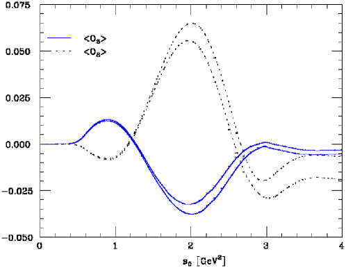
Los resultados para los condensados de vacio de la Cromodinámica Cuántica obtenidos en la presente tesis doctoral, como función del parámetro de integración $s_{0}$. Las bandas de error corresponden a incertidumbres de 1-$\sigma$ que provienen de la parametrización de $\rho_{V-A}(s)$.

En la segunda de las aplicaciones descritas en el Capítulo 6, generalizamos los resultados de [f2ns], referidos a la parametrización de funciones de estructura $F(x,Q^{2})$, construyendo una parametrización de estas funciones en colisiones profundamente inelásticas del protón que incluye todos los datos experimentales de que se dispone, en particular las medidas de alta precisión del experimento HERA, especialmente en la región de pequeño $x$. En la fig. 2.3 podemos ver el resultado de este análisis comparado con los resultados originales obtenidos en [f2ns]. Notemos como en la región cinemática donde los datos experimentales incluidos en los dos análisis se solapan, que es la que corresponde a valores grandes de la variable $x$, los dos resultados son perfectamente consistentes, como era de esperar.

Figure 2.3:

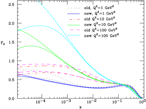
Los resultados para la función de estructura del protón $F_{2}^{p}(x,Q^{2})$ obtenidos en la presente tesis doctoral comparados con los resultados originales [f2ns].

En tercer lugar, estudiamos las desintegraciones semileptónicas del mesón B, comparamos nuestros resultados con una serie de resultados teóricos y extraemos de la parametrizacion del espectro energético del leptón la masa del quark b, $m_{b}$. La determinación de parámetros no perturbativos, como las masas de los quarks pesados o los elementos de la matriz de CKM, son una de las principales motivaciones para los análisis teóricos y experimentales de las desintegraciones de los mesones B. En la Fig. 2.4 mostramos los resultados obtenidos para la parametrización del especto leptónico, para diferentes combinaciones de experimentos incluidos en el fit, como se describe en detalle en la sección 6.3.

Figure 2.4:

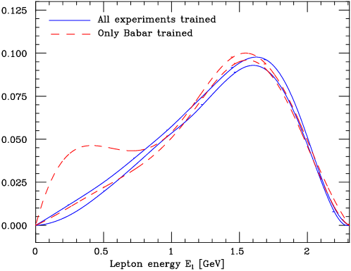
Comparación de los resultados para la parametrización del espectron energético leptónico con todos los experimentos incorporados en el fit, con el caso en que solamente los datos del experimento Babar han sido considerados.

Esta aplicación demuestra como nuestra técnica general para parametrizar datos experimentales se puede aplicar a la reconstrucción de una función si la única información experimental accesible procede de integrales truncadas de esta función. Esto permite una comparación más general de las predicciones teóricas con los datos experimentales, sin necesidad de hipótesis adicionales y con una estimación fidedigna de los errores experimentales. Asimismo, el desarrollo de estas técnicas permitirá en un futuro aplicarlas a otras situaciones de interés en física de mesones B, como por ejemplo la parametrización de la shape function $S(\omega)$, que contiene los efectos no perturbativos dominantes en una serie de procesos como las desintagraciones radiativas de los mesones B.

La aplicación más imporante de todas es descrita en la última sección del Capítulo 6: la parametrización de distribuciones de partones. Primero describimos una nueva técnica para implementar la dependencia con la energía $Q^{2}$ de estas distribuciones, y seguidamente describimos la construcción de la densidad de probabilidad en el espacio de las distribuciones de partones non-singlet, a partir de datos experimentales de funciones de estructura. En la Fig. 2.5 podemos observar los resultados para la distribución de partones nonsinglet obtenida en la presente tesis doctoral con dos valores diferentes $Q_{0}^{2}$ del corte cinématico. Este corte cinemático es debido a que solo los datos experimentales de la función de estructura $F_{2}^{NS}(x,Q^{2})$ con $Q^{2}$ suficientemente grande pueden tratarse mediante la teoría de perturbaciones de la Cromodinámica Cuántica.

Figure 2.5:

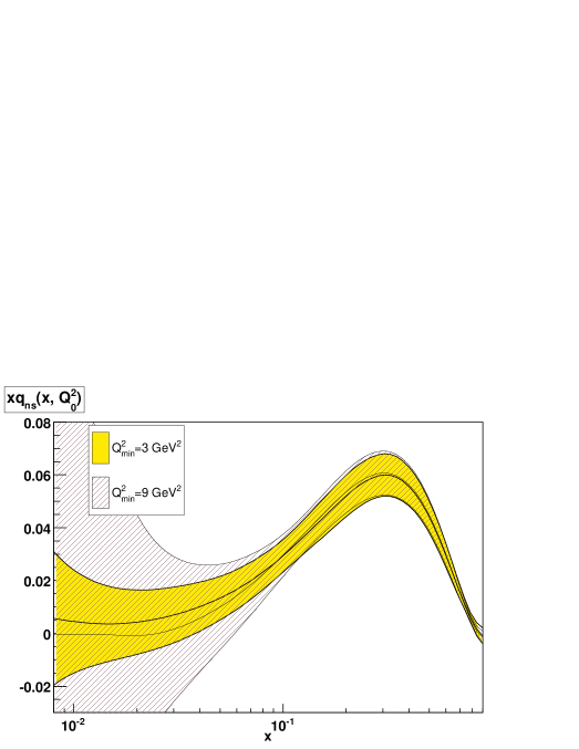
Comparación de los resultados para la distribucion de partones $xq_{NS}(x,Q_{0}^{2})$ para dos valores diferentes del corte cinemático: el de referencia $Q^{2}\geq 3$ GeV${}^{2}$, con uno más conservativo $Q^{2}\geq 9$ GeV${}^{2}$.

En la Fig. 2.6 tenemos el esquema del proceso utilizado en la parametrización de la distribución de partones non-singlet, a partir de datos experimentales de las funciones de estructura en colisiones profundamente inelásticas. Recordemos los tres pasos principales de nuestra técnica descrita anteriormente, como pueden verse en la Fig. 2.6: generación Monte Carlo de replicas de las medidas experimentales, entrenamiento de redes neuronales artificiales que parametrizan la distribución de partones non-singlet y finalmente la validación estadística de los resultados.

Figure 2.6:

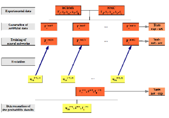
Estrategia general seguida para la parametrización de la distribución de partones non-singlet $q_{NS}(x,Q^{2}_{0})$ a partir de datos experimentales de la función de estructura $F_{2}^{NS}(x,Q^{2})$.

Las técnicas descritas en la Sección LABEL:nnqns_appl proporcionan la base para la realización de una parametrización de todas la distribuciones de partones, incluyendo el gluon, que son necesarias para aplicaciones fenomenológicas generales. En particular, es directo extender el formalismo de evolución que describiremos en el caso de las distribuciones nonsinglet al caso general con combinaciones arbitrarias de distribuciones de partones. De la misma manera, los datos experimentales que se usan en este caso son los del análisis de la Sección 6.2, esto es, la parametrización de la función de estructura del protón $F_{2}^{p}(x,Q^{2})$. Por lo tanto, con los resultados obtenidos en la presente tesis doctoral se tienen todos los ingredientes necesarios para obtener un set de todas las distribuciones de partones con la técnica descrita en el Capítulo 5.

Finalmente, tras las conclusiones de la presente tesis doctoral, dos apéndices incluyen material de referéncia sobre análisis estadístico de los datos experimentales y sobre el estado actual de las determinaciones de las distribuciones de partones. En el primer apéndice, dedicado al tratamiento estadístico de los datos experimentales, describimos con un modelo sencillo que se puede resolver exactamente las propiedades de los diferentes estimadores usados para el entrenamiento de las redes neuronales, así como los efectos de un tratamiento incorrecto de los errores de normalización. En el segundo apéndice resumimos el estado actual de las determinaciones globales de distribuciones de partones, analizando con detalle las características de los análisis de las dos colaboraciones más importantes, CTEQ y MRST, junto con los datos experimentales y las parametrizaciones de las distribuciones de partones utilizadas en cada caso.

Chapter 3 Introduction and motivation

The Large Hadron Collider (LHC) is a proton-proton collider at center of mass energy $\sqrt{s}=14~{}$TeV which is located at the Organisation Européenne pour la Recherche Nucléaire (CERN), near Genève in Switzerland (see Fig. 3.1). Its construction is almost finished, and it is scheduled to deliver the first collisions by the end of 2007. The energies that will be achieved at the LHC will allow us to probe the smallest distances ever and will open a new era for particle physics, since it will investigate the true nature of electroweak symmetry breaking, and hopefully will deliver invaluable information of new physics beyond the Standard Model (SM) of particle interactions. However, possible new physics signals will appear together with a far more copious background from Standard Model processes, essentially from the interactions of quarks and gluons within the proton as determined by Quantum Chromodynamics (QCD), the sector of the SM that describes the strong interaction.

Therefore, the discovery potential of LHC as well as its ability to also perform precision measurements of the new physics properties depends crucially on the understanding of the huge Standard Model background. Since the LHC is an hadron collider, to be able to perform precision predictions for different observables one needs first to understand quantitatively the underlying strong interaction processes and the associated uncertainties. Among these uncertainties, one of the most important ones comes from the parton distribution functions, which measure the momentum distribution of quarks and gluons inside the protons. Parton distributions cannot be computed from first principles, but rather they need to be extracted from experimental data from other hard scattering processes, like for example deep inelastic scattering.

Figure 3.1:

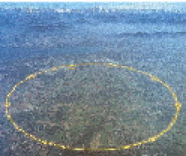
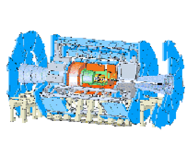
The location of the LHC experiment near Gèneve (left) and the one of its detectors, ATLAS (right).

Parton distribution functions $q_{i}(x,Q_{0}^{2})$ can be determined from experimental data by means of the QCD factorization theorem, which states that any hard-scattering cross section can be separated into a process-dependent coefficient and a set of universal, process-independent parton distribution functions. That is, the factorization theorem relates observables like deep-inelastic scattering structure functions $F(x,Q^{2})$ to a convolution of short-distance coefficient functions, $C_{i}\left(x,\alpha_{s}\left(Q^{2}\right)\right)$, which can be computed in perturbation theory, and parton distribution functions,

$$F(x,Q^{2})=C_{i}\left(x,\alpha_{s}\left(Q^{2}\right)\right)\otimes q_{i}(x,Q^{2})\ .$$ (3.1)

The dependence with the scale $Q^{2}$ of the parton distributions is determined in QCD perturbation theory from the so-called parton evolution equations. Note that in general different combinations of parton distributions contribute to different observables. The inclusion of a wide variety of hard-scattering data is thus crucial to disentangle the various parton distributions. Even if the backbone of the determinations of parton distributions is the high precision deep-inelastic scattering data, essential experimental input comes from other measurements like jet production, heavy boson production or the Drell-Yan process. In Fig. 3.2 we show the set of parton distribution functions from a recent global QCD analysis.

Figure 3.2:

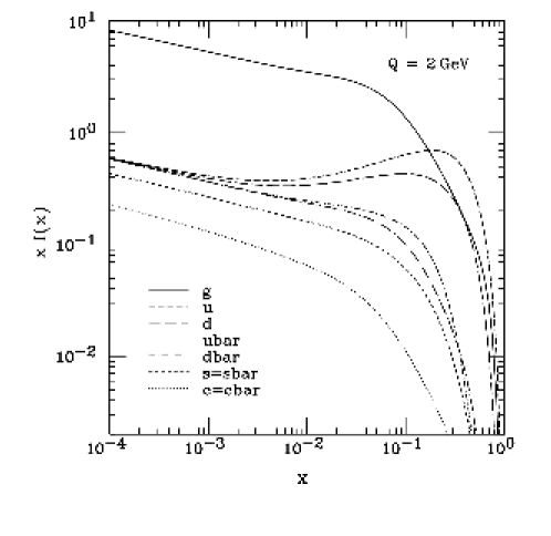
Parton distribution functions $q_{i}(x,Q_{0}^{2})$ as determined from experimental data in a recent QCD global analysis [cteq61].

The requirements of precision physics at hadron colliders, specially the Large Hadron Collider, determine that it is now mandatory to determine accurately not only the parton distributions themselves but also the uncertainties associated to them. Note that a detailed knowledge of parton distributions and their associated uncertainties is essential if one wants to perform accurate measurements, since a typical LHC cross-section $\sigma(x,Q^{2})$ reads

$$\sigma(x,Q^{2})=C_{ij}\left(x,\alpha_{s}\left(Q^{2}\right)\right)\otimes q_{i}(x,Q^{2})\otimes q_{j}(x,Q^{2})\ ,$$ (3.2)

which involves the product of two parton distributions from each of the two partons in the initial state of the proton-proton collision. The problem is specially acute since the kinematic region covered by the LHC overlaps only partially with the kinematical range of those experiments used to determine the parton distributions, like HERA, as can be seen in Fig. 3.3, and therefore one has to extrapolate parton distribution into an unknown kinematical region. Also for this reason it is essential to determine the uncertainties in parton distributions and propagate them into the extrapolation region probed by LHC.

Figure 3.3:

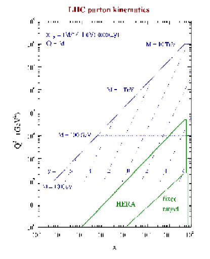
The kinematical coverage of the LHC compared to that of the HERA collider and fixed target deep-inelastic scattering experiments.

The main problem to be faced here is that one is trying to determine an uncertainty on a function, i.e., a probability measure on a space of functions, and to extract it from a finite set of experimental data. Within the framework of the standard approach to determine parton distributions from experimental data, several techniques have been constructed to assess these uncertainties. However, even if all these techniques have been useful to estimate the size of the uncertainties, they suffer from several drawbacks. First of all, since in the standard approach parton distributions are parametrized with relatively simple functional forms like

$$q_{i}(x,Q_{0}^{2})=A_{i}x^{b_{i}}(1-x)^{c_{i}}\left(1+d_{i}x+e_{i}x^{2}+\ldots\right)\ ,$$ (3.3)

where the parameters $A_{i},b_{i},\ldots$ are fitted from experimental data, the estimation of the uncertainties is restricted to the space parametrized by Eq. 3.3 and therefore depends heavily on the assumptions done for the non-perturbative shapes of the parton distributions. Second, in order to propagate the uncertainties in the parton distributions to an arbitrary observable, linearized approximations in the error propagation have to be used, whose validity is at best doubtful. Finally, in the presence of experimental data from different experiments, it has been argued that incompatibility between different experiments force that the tolerance condition in the $\chi^{2}$ used to estimate the errors is not the textbook value $\Delta\chi^{2}=1$ but a much larger value $\Delta\chi^{2}=50$ or 100. Even if this choice can be justified to some extent, in practice parton uncertainties determined with this condition lose their statistical meaning, since they depend on the choice of the free parameter $\Delta\chi^{2}$.

Therefore, in view of the crucial importance of parton distribution functions for LHC precision physics, it is worth investigating alternative approaches for the determination of parton distributions and the associated uncertainties that bypass the problems of the standard approach discussed above. In Ref. [f2ns] a novel technique was presented to determine the associated probability measure in the space of a function, which was applied to the parametrization of deep inelastic structure functions. This technique uses a combination of Monte Carlo samplings of the experimental data together with artificial neural networks as universal unbiased interpolants. The use of neural networks instead of fixed functional forms as in Eq. 3.3 avoids the bias introduced by the assumption of a given functional form, and the Monte Carlo sampling provides a statistically rigorous estimation of the function uncertainties, which allows for a general error propagation to arbitrary observables without the need of linearized approximations.

In this thesis we extend the work of Ref. [f2ns] in different ways: first we have applied the general strategy to parametrize experimental data to other processes of interest, in particular to the case of parton distribution functions. In all these cases the relation between the parametrized quantity and the experimental data was completely different, so it has been shown that the approach of Ref. [f2ns] is suited for a variety of situations. Second, we have extended the basic technique with the introduction of new minimization algorithms, specially genetic algorithms, as well as new statistical estimators to assess the stability of the obtained probability measure in different aspects. Finally, several improvements of the neural network training have been introduced to optimize its efficiency.

The outline of the present thesis is as follows. In Chapter 4 we review the basic elements of Quantum Chromodynamics, as well as those high energy processes that will be used later in the thesis. We present also a review of the standard approach to parametrize parton distribution functions with their associated uncertainties. In Chapter 5 we introduce the general technique to parametrize experimental data in an unbiased way with faithful estimation of the uncertainties, which is the main subject of this thesis. Then in Chapter 6 we present four applications of the general strategy, and special attention is paid to the most important one, the parametrization of the nonsinglet parton distribution. Two appendices summarize background material on statistical analysis of experimental data and on the current status of the standard approach to global fits of parton distributions.

Chapter 4 Elements of perturbative QCD and global parton distributions analysis

In this first Chapter we review the basic elements of Quantum Chromodynamics (QCD), the gauge theory of the strong interactions. After a brief description of the theoretical foundations of QCD, we describe in some detail the deep-inelastic scattering process. This process is the most important source of information on parton distribution functions, whose parametrization, as we have discussed in the Introduction, is the main motivation for the set of techniques developed in the present thesis. We will consider also two other high energy processes, since they have provided testing grounds for our strategy to parametrize experimental data: the semileptonic decays of the B meson and the hadronic tau decays.

Parton distribution functions, as has been discussed in the Introduction, have to extracted from experimental data, by means of a QCD analysis of a variety of hard scattering measurements. In the second part of this Chapter we present a summary of the standard approach to global fits of parton distributions, and we discuss in some detail the different methods, with their advantages and drawbacks, which are commonly used to estimate the associated uncertainties of parton distribution functions.

4.1 Overview of perturbative QCD

4.1.1 Basics of Quantum Chromodynamics

Quantum Chromodynamics (QCD) is the gauge theory that describes the strong interaction (see for example Refs. [collider, handbook] and references therein). Gauge invariance under the group SU(N) and renormalizability determine completely the form of the Lagrangian. The QCD Lagrangian describes the strong interaction between quarks and gluons, and it reads

$$\mathcal{L}_{\mathrm{QCD}}=\sum_{i=1}^{N_{f}}\bar{q}_{i}\left(i\gamma^{\mu}D_{\mu}-m_{i}\right)q_{i}-\frac{1}{4}F_{\mu\nu}^{A}F_{\mu\nu}^{A}\ .$$ (4.1)

Let us describe the elements of the above equation. The $N_{f}$ spinor quark fields of different flavor are labeled by $q_{i}$, each with mass $m_{i}$. The Dirac matrices $\gamma^{\mu}$ appear due to the fermionic nature of quarks, and are defined by the anticommutation relation $\{\gamma^{\mu},\gamma^{\nu}\}=2g^{\mu\nu}$. The covariant derivative reads in terms of the gluon field $A_{\mu}^{A}$

$$\left(D_{\mu}\right)_{ab}=\partial_{\mu}\delta_{ab}+ig\left(t^{A}A^{A}_{\mu}\right)_{ab}\ ,$$ (4.2)

where $\mu$ is a Lorentz index, $\mu=0,1,2,3$, and $a,b$ are color indices for the fundamental representation, $a,b=1,\ldots,N$. The matrices $t^{A}$, where $A$ is a color index in the adjoint representation, $A=1,\ldots,N^{2}+1$, are the SU(N) generating matrices in the fundamental representation. The last term in Eq. 4.1 is the field-strength tensor for the gluon field,

$$F_{\mu\nu}^{A}=\partial_{\mu}A_{\nu}^{A}-\partial_{\nu}A^{A}_{\mu}-gf^{ABC}A^{B}_{\mu}A^{C}_{\nu}\ ,$$ (4.3)

where $f^{ABC}$ are the structure constants of SU(3), defined by the commutation relation

$$\left[t^{A},t^{B}\right]=if^{ABC}t^{C}\ .$$ (4.4)

The last term in Eq. 4.3 describes the self-interaction of the gluons, a typical feature of non-abelian gauge theories like QCD which renders the theory asymptotically free, as discussed below. Finally, $g$ is the QCD coupling constant, which is, together with the quark masses, the only free parameter of the theory.

From this Lagrangian, using standard rules of Quantum Field Theory [peskin] one can compute several observables, like cross sections or decay rates, in a perturbative series expansion in powers of $\alpha_{s}=g^{2}/4\pi$. Radiative quantum corrections induce a dependence of the strong coupling with respect to the typical energy of the process $E$, which at lowest order reads

$$\alpha_{s}=\alpha_{s}(E)=\frac{1}{\beta_{0}\ln\frac{E^{2}}{\Lambda^{2}_{\mathrm{QCD}}}}\ ,$$ (4.5)

where $\beta_{0}$ is the first coefficient of the QCD $\beta$ function that determines the running of $\alpha_{s}$ with the energy. The main feature of QCD can be seen from Eq. 4.5: the theory is asymptotically free [gross, politzer], which means that the coupling constant vanishes when the typical energies of the process become very large with respect to the typical scale of the theory, $\Lambda_{\mathrm{QCD}}$. Asymptotic freedom allows us to apply QCD to many high energy processes for which perturbation theory is meaningful, since in this case $E\gg\Lambda_{\mathrm{QCD}}$ and therefore $\alpha_{s}(E)\ll 1$. On the other hand, the same asymptotic freedom property implies that the theory becomes strongly coupled at low energies, $E\leq\Lambda_{\mathrm{QCD}}$, and in this non-perturbative regime the standard tools of perturbation theory are useless, and one has to resort to other methods, like lattice computations [lattice]. In Fig. 4.1 we show a comparison of different extractions of the strong coupling $\alpha_{s}(E)$ with the theoretical QCD predictions [bethke].

Figure 4.1:

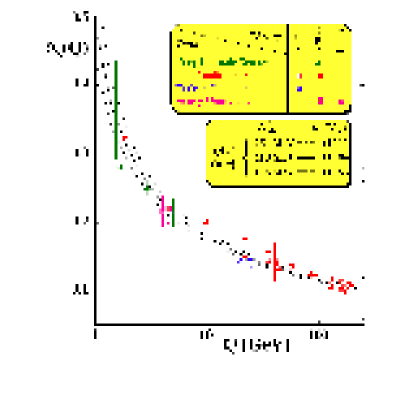
Comparison of different determinations of the strong coupling $\alpha_{s}(Q)$ at several energies $Q$ from a variety of processes, as summarized in Ref. [bethke].

For single scale observables, that is, for processes which depend only on a single hard scale $Q^{2}$ (where again a hard scale is a energy scale which satisfies the condition $Q^{2}\gg\Lambda_{\mathrm{QCD}}$), the perturbative expansion in powers of the strong coupling reads, for those processes in which we are interested in,

$$R(Q^{2})=\sum_{n=1}^{\infty}a_{n}\alpha_{s}\left(Q^{2}\right)^{n}\ ,$$ (4.6)

where without loss of generality we have assumed that the perturbative expansion of the observable $R(Q^{2})$ starts at order $\alpha_{s}\left(Q^{2}\right)$. The best example of this first case is the total cross section of $e^{+}e^{-}$ going to hadrons, where in this case the hard scale is identified with the center of mass energy of the collision, $Q^{2}=s$.

Perturbative expansions become more complicated as the number of hard scales present in the process begins to increase. In this case it is not always true that observables can be expanded in a simple power series in $\alpha_{s}\left(Q^{2}\right)$. Let us consider to be definite the deep-inelastic scattering processes, which is the best known example of a two-scale process, and which will be discussed in detail in the next Section. In this case the two hard scales will be denoted by $Q^{2}$ and $W^{2}$. In deep-inelastic scattering, as we will see in brief, the nonsinglet structure function at leading order is given by

$$F_{2}^{NS}(N,Q^{2})=\left[\frac{\alpha_{s}\left(Q^{2}\right)}{\alpha_{s}\left(Q^{2}_{0}\right)}\right]^{\gamma(N)/\beta_{0}}\ ,$$ (4.7)

where $N$ is the conjugate variable of the ratio $x=Q^{2}/(Q^{2}+W^{2})$, and therefore $F_{2}^{NS}$ cannot be expanded in integer powers of $\alpha_{s}\left(Q^{2}\right)$. Another example is the singlet structure function at small $x$ [das], which reads

$$F_{2}(x,Q^{2})\Bigg{|}_{x\to 0}\sim\exp\left(\sqrt{\ln\left(1/x\right)\ln\ln\left(\alpha_{s}\left(Q^{2}\right)\right)}\right)\ ,$$ (4.8)

which again is not expandable in a simple series in powers of $\alpha_{s}\left(Q^{2}\right)$.

In some cases, however, perturbative computations which depends on two hard scales have a perturbative expansion of a similar form of Eq. 4.6, that is, a expansion in integer powers of the strong coupling, like the deep-inelastic scattering coefficient functions, which are of the form

$$C(Q^{2},W^{2})=\sum_{k=1}^{\infty}\alpha_{s}\left(Q^{2}\right)^{k}b_{k}\left(\frac{Q^{2}}{W^{2}}\right)\ .$$ (4.9)

Note that unlike Eq. 4.6 the coefficients of the expansion $b_{k}$ are not pure numbers but functions of the ratio of scales $Q^{2}/W^{2}$. In these coefficients $b_{k}$ one can encounter large logarithmic terms of the form $\left(\ln Q^{2}/W^{2}\right)^{p}$. These logarithmic terms can become large in some kinematical regions and need to be resummed to all orders [sterman] in order to trust perturbation theory. Note that typical perturbative expansions like Eq. 4.6 and 4.9 are at best asymptotic expansions, and often their large order behavior introduces divergences, leading to ambiguities in the value of the summed perturbative expansion related to nonperturbative corrections [renormalons]. Note also that since the coupling $\alpha_{s}\left(Q^{2}\right)$ increases as the value $Q^{2}$ decreases, the perturbative expansions Eqs. 4.6 and 4.9 are meaningful only for large enough values of $Q^{2}\gg\Lambda_{\mathrm{QCD}}$, that is, for the so-called hard processes [harddok].

The foundation for results like Eq. 4.6 and 4.9 is the Operator Product Expansion. This expansion allows to organize any quantity in a series in inverse powers of $Q^{2}$, the typical energy scale of the process, by means of an expansion of composite operators in terms of simpler operators of the appropiate dimension. The Operator Product Expansion [svz] can be used to parametrize higher-order nonperturbative effects that are mostly relevant at low $Q^{2}$ in terms of matrix elements of local operators, and in this way to extend the validity range of theoretical predictions. For example, for a single scale observable, the operator product expansion reads schematically

$$R\left(Q^{2}\right)=\sum_{k=0}^{\infty}c_{k}\left(\alpha_{s}\left(Q^{2}\right)\right)\frac{\left\langle\mathcal{O}_{k}\right\rangle}{Q^{k}}\ ,$$ (4.10)

where $\left\langle\mathcal{O}_{k}\right\rangle$ are nonperturbative expectation values of operators with the appropriate dimensions, and where the leading order result corresponds to the unit operator, $\mathcal{O}_{0}=1$,

$$c_{0}\left(\alpha_{s}\left(Q^{2}\right)\right)=\sum_{n=1}^{\infty}a_{n}\alpha_{s}\left(Q^{2}\right)^{n}\ .$$ (4.11)

It is clear from Eq. 4.10 that at large enough values of $Q^{2}$ only the leading term in the OPE is relevant for phenomenological purposes. The nonperturbative matrix elements $\left\langle\mathcal{O}_{k}\right\rangle$ in Eq. 4.10 can be extracted from experimental data in some processes and then be used in other processes to increase the accuracy of the theoretical prediction, as in the case of parton distribution functions, which will be analyzed in detail in Section 4.1.2.

Now we review the high energy processes that will be used in applications of the general technique to parametrize experimental data which is the main subject of this thesis: deep-inelastic scattering, semileptonic B meson decays and hadronic tau decays.

4.1.2 Deep-inelastic scattering

For a variety of reasons deep-inelastic scattering (DIS), the high energy scattering of leptons and hadrons, is one of the most important processes in Quantum Chromodynamics. The original, and still the most powerful, test of perturbative QCD is the breaking of Bjorken scaling [bjorken] in DIS, that is, the logarithmic dependence of deep-inelastic structure functions with the momentum transfer $Q^{2}$. Nowadays, deep inelastic structure functions analyses not only provide some of the most precise tests of the theory but also determine the momentum distributions of partons in hadrons, which are an essential input in predicting cross section in high energy hadron collisions.

Deep-inelastic scattering is probably the best theoretically understood process in perturbative QCD. The full next-to-next-to-leading order computation was recently finished [mvvs, mvvns], and also threshold resummation at the next-to-next-to-leading logarithmic accuracy can be implemented [sudakovho]. On the experimental side, deep inelastic scattering is the high energy process involving strongly interacting particles which has been measured experimentally with the highest accuracy. For example, the lepton-proton collider HERA [herarev] has measured deep-inelastic scattering cross-sections with 1% accuracy in a wide kinematical range.

Moreover, as we have mentioned before, deep-inelastic scattering is essential to be able to use perturbative QCD in other processes involving hadrons in the initial state, like proton-proton collisions at the LHC. This is so because deep-inelastic scattering provides the backbone information on the parton distribution functions (PDFs) of the nucleon [heralhc]. As will be discussed in more detail, a detailed knowledge of parton distribution functions and its associated uncertainties is an essential input for precision LHC phenomenology.

Now we present the basic formulae that describe deep-inelastic scattering, and that will be useful in Chapter 6. Deep-inelastic scattering is the high-energy collision of a lepton (an electron, a muon or a neutrino) against a hadronic target (a proton or a nucleus). The kinematics of this process (see Fig. 4.2) are determined in terms of two variables $x$ and $Q^{2}$, defined as

$$x=\frac{Q^{2}}{2p\cdot q},\qquad Q^{2}=-q^{2}\ ,$$ (4.12)

where $q$ is the momentum carried by the virtual gauge boson and $p$ is the momentum carried by the incoming proton. Other important variables are the invariant mass of the final hadronic state $W^{2}$ and the inelasticity $y$, given by

$$W^{2}=Q^{2}\frac{1-x}{x}\ ,\qquad y=\frac{q\cdot p}{k\cdot p}\ ,$$ (4.13)

where $k$ is the momentum carried by the initial state lepton. The applicability of perturbation theory requires that both scales $Q^{2}$ and $W^{2}$ are large, because if not either higher twist corrections are relevant, or the perturbative expansion breaks down due to the presence of large logarithms of the form $\alpha_{s}\left(Q^{2}\right)^{p}\ln^{k}(1-x)$. The kinematical cut in $W^{2}$ can be lowered by including the effects of threshold resummation [corcellaresum]. Note that even if $Q^{2}$ is large, $W^{2}$ can be small provided $x$ is large enough. The relation between perturbative threshold resummation and higher twist nonperturbative corrections is still an open issue [landau].

Figure 4.2:

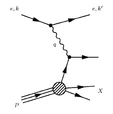
The deep-inelastic scattering process: the hard scattering of a lepton off a hadron, typically a proton.

The deep-inelastic scattering cross section can be decomposed using kinematics and Lorentz invariance in terms of structure functions $F_{i}(x,Q^{2})$. These structure functions parametrize the structure of the proton as seen by the virtual gauge boson. If the incoming lepton is a charged lepton (an electron or a muon) then for $Q^{2}\ll M_{Z}^{2}$ the double differential deep-inelastic scattering cross section reads

$$\frac{d^{2}\sigma^{\mathrm{em}}}{dxdQ^{2}}=\frac{4\pi\alpha^{2}}{Q^{4}}\left[\left(1+(1-y)^{2}\right)F_{1}(x,Q^{2})+\frac{1-y}{x}\left(F_{2}(x,Q^{2})-2xF_{1}(x,Q^{2})\right)\right]\ ,$$ (4.14)

where $\alpha$ is the electromagnetic coupling. If the incoming lepton is a neutrino, then the cross section reads

$$\frac{d^{2}\sigma^{\nu p}}{dxdy}=\frac{G_{F}^{2}ME}{\pi}\left[\left(1-y-\frac{M}{2E}xy\right)F_{2}^{\nu}(x,Q^{2})+y^{2}xF_{1}^{\nu}(x,Q^{2})+y\left(1-\frac{y}{2}\right)xF_{3}^{\nu}(x,Q^{2})\right]\ .$$ (4.15)

where $G_{F}$ is the Fermi constant, $M$ the mass of the target hadron and $E$ the neutrino energy in the hadron rest frame. Note that Eq. 4.15 holds both for charged current ($W^{\pm}$ exchange) and neutral current ($Z$ exchange) neutrino scattering, even if the decomposition of the structure functions $F_{i}^{\nu}(x,Q^{2})$ in terms of parton distributions is different in the two cases [neutdis]. All the structure functions defined above have been measured in several experiments, and the most precisely known is the charged lepton scattering neutral current structure function $F_{2}(x,Q^{2})$, thanks to the high precision measurements at HERA and in fixed target experiments. In Fig. 4.3 we show a summary of available data on this structure function from different experiments. Note that the effects of QCD evolution, that is, the dependence of $F_{2}(x,Q^{2})$ with the scale $Q^{2}$, is clearly observed in the experimental data, specially in the small-$x$ region.

Figure 4.3:

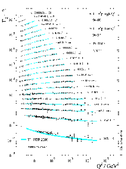
The deep-inelastic structure function $F_{2}^{p}(x,Q^{2})$ as measured by several different experiments (HERA, BCDMS and NMC). Note the dependence of $F_{2}^{p}(x,Q^{2})$ with $Q^{2}$, as dictated by perturbative QCD.

Structure functions $F_{i}(x,Q^{2})$ depend on the momentum distribution of partons (quarks and gluons) inside the proton, which are determined by low energy nonperturbative dynamics, and therefore cannot be computed in perturbation theory. However, each structure function $F_{i}(x,Q^{2})$, using the factorization theorem [factorization], can be written as a convolution of hard-scattering coefficients $C_{ij}(x,\alpha_{s}(Q^{2}))$, which depend only on the short-distance (perturbative) physics, and parton distribution functions $q_{j}(x,Q^{2})$ [partonsalt], which parametrize the (non-perturbative) structure of the proton. The factorized structure function reads

$$F_{i}(x,Q^{2})=\int_{x}^{1}\frac{dy}{y}C_{ij}(y,\alpha_{s}(Q^{2}))q_{j}\left(\frac{x}{y},Q^{2}\right)\ .$$ (4.16)

The coefficient functions $C_{i}(x,\alpha_{s}(Q^{2}))$ can be computed in perturbation theory as a power series expansion in $\alpha_{s}(Q^{2})$. Parton distribution can be formally defined [collinspdf] by means of suitable operator matrix elements in the proton,

$$q_{i}\left(x,Q^{2}\right)\equiv\int\frac{dy^{-}}{4\pi}e^{-ixp^{+}y^{-}}\left\langle p|\bar{\psi}_{i}\left(0,y^{-}\right)W[y,0]\gamma^{+}\psi(0)|p\right\rangle_{R}\ ,$$ (4.17)

where $W[y]$ is a Wilson line (a path-ordered exponential of the gluon field) and the parton distributions are renormalized at the scale $\mu^{2}=Q^{2}$. Since these parton distributions are non-perturbative, they must be determined from experimental data. The techniques used to extract parton distributions from hard scattering data together with the associated uncertainties will be discussed in the next Section.

At leading order in the strong coupling $\alpha_{s}\left(Q^{2}\right)$, the expressions for the different structure functions in terms of parton distribution functions are relatively simple. For example, for charged lepton scattering off a proton target one has

$$F_{2}^{\mathrm{em}}(x,Q^{2})=x\left[\frac{4}{9}\left(u+\bar{u}+c+\overline{c}\right)+\frac{1}{9}\left(d+\bar{d}+s+\overline{s}\right)\right]\left(x,Q^{2}\right)\ ,$$ (4.18)

$$2xF_{1}(x,Q^{2})=F_{2}(x,Q^{2})\ ,$$ (4.19)

where the last relation is the Callan-Gross relation [callangross]. The parity violating structure function $xF_{3}$ in charged lepton scattering can be neglected in the $Q^{2}\ll M_{Z}^{2}$ limit, since only contains contributions from Z boson exchange. For neutrino-proton scattering the appropriate relations are given by

$$F_{2}^{\nu}(x,Q^{2})=2x\left[d+s+\bar{u}+\bar{c}\right]\left(x,Q^{2}\right)\ ,$$ (4.20)

$$xF_{3}^{\nu}\left(x,Q^{2}\right)=2x\left[d+s-\bar{u}-\bar{c}\right]\left(x,Q^{2}\right)\ .$$ (4.21)

In the above expressions, $u(x,Q^{2})$ is the parton distribution function of the u-quark in the proton, $d(x,Q^{2})$ that of the d-quark, and so on.

At very high energies, $Q^{2}\geq M_{Z}^{2}$, one has to take into account the contribution of $Z$ boson exchange in neutral current charged lepton scattering. The generalization of Eq. 4.14 which incorporates the complete neutral current exchange is given by

$$\frac{d^{2}\sigma}{dxdQ^{2}}=\frac{4\pi\alpha^{2}}{xQ^{4}}\left[xy^{2}F_{1}^{NC}(x,Q^{2})+(1+y)F_{2}^{NC}(x,Q^{2})+y\left(1-\frac{y}{2}\right)F_{3}^{NC}(x,Q^{2})\right]\ ,$$ (4.22)

where in terms of parton distribution functions one has

$$F_{2}^{NC}(x)=2xF_{1}^{NC}(x)=\sum_{i=1}^{N_{f}}\left[q_{i}(x)+\bar{q}_{i}(x)\right]C_{q}(Q^{2})\ ,$$ (4.23)

$$xF_{3}^{NC}(x)=\sum_{i=1}^{N_{f}}\left[q_{i}(x)-\bar{q}_{i}(x)\right]D_{q}(Q^{2})\ ,$$ (4.24)

$$C_{q}(Q^{2})=e_{q}^{2}-2e_{q}V_{e}V_{q}P_{Z}+(V_{e}^{2}+A_{e}^{2})(V_{q}^{2}+A_{q}^{2})P_{Z}^{2}\ ,$$ (4.25)

$$D_{q}(Q^{2})=-2e_{q}^{2}A_{e}A_{q}P_{Z}+4V_{e}A_{e}V_{q}A_{q}P_{Z}^{2},\qquad P_{Z}=\frac{Q^{2}}{Q^{2}+M_{Z}^{2}}\ ,$$ (4.26)

where $e_{i}$ are the electromagnetic charges of the quarks and $V_{i}$ and $A_{i}$ are the vector and axial couplings of the fermions to the Z boson. Note the appearance of the parity-violating structure function $F_{3}(x,Q^{2})$, which is sensitive to the helicity of the incoming leptons (that is, it is different for example for an electron and for a positron).

Even if parton distribution functions $q_{i}(x,Q_{0}^{2})$ are of non-perturbative origin, it can be shown that their dependence with the scale $Q^{2}$ is dictated by perturbative QCD, provided the scale $Q^{2}$ is large enough. The dependence of the parton distributions with the scale $Q^{2}$, also known as their evolution with $Q^{2}$, is dictated by the perturbative DGLAP [gl, dok, ap] evolution equations. These equations can be used to evolve with $Q^{2}$ any combination of parton distributions, however, their form is much simpler if suitable combinations are defined. For nonsinglet combinations of parton distributions, defined as differences between quark distributions,

$$q_{NS,ij}(x,Q_{0}^{2})\equiv\left(q_{i}-q_{j}\right)(x,Q^{2}_{0})\ ,$$ (4.27)

where $i,j$ label either a quark or an antiquark, the DGLAP evolution equation reads

$$\frac{dq_{NS}(x,Q^{2})}{d\ln Q^{2}}=\frac{\alpha_{s}(Q^{2})}{2\pi}\int_{x}^{1}\frac{dy}{y}P_{NS}\left(y,\alpha_{s}(Q^{2})\right)q_{NS}\left(\frac{x}{y},Q^{2}\right)\ ,$$ (4.28)

where $P_{NS}(x,\alpha_{s}\left(Q^{2}\right))$ are the non-singlet splitting functions. These splitting functions can be computed perturbatively as an expansion in powers of $\alpha_{s}\left(Q^{2}\right)$. For instance, the leading order expression for the nonsinglet splitting function is given by

$$P_{NS}^{(0)}\left(x\right)=C_{F}\left(\frac{1+x^{2}}{(1-x)_{+}}+\frac{3}{2}\delta(1-x)\right)\ .$$ (4.29)

It is clear from its definition that the gluon is decoupled from the evolution of nonsinglet parton distributions. The remaining independent combination of parton distribution is called the singlet parton distribution, defined as the sum of all quark and anti-quark flavors,

$$\Sigma(x,Q^{2})\equiv\sum_{i=1}^{N_{f}}\left(q_{i}(x,Q^{2})+\overline{q}_{i}(x,Q^{2})\right)\ .$$ (4.30)

In the singlet sector, the DGLAP equation is a 2-dimensional matrix equation. In this case the singlet distribution evolves coupled to the gluon parton distribution using the singlet DGLAP evolution equation,

$$\frac{d}{d\ln Q^{2}}\left(\begin{array}[]{c}\Sigma(x,Q^{2})\\ g(x,Q^{2})\end{array}\right)=\frac{\alpha_{s}(Q^{2})}{2\pi}\int_{x}^{1}\frac{dy}{y}\left(\begin{array}[]{cc}P_{qq}(y)&P_{qg}(y)\\ P_{gq}(y)&P_{gg}(y)\end{array}\right)\left(\begin{array}[]{c}\Sigma(x/y,Q^{2})\\ g(x/y,Q^{2})\end{array}\right)\ ,$$ (4.31)

in terms of the singlet matrix of splitting functions.

The DGLAP evolution equations, Eqns. 4.28 and 4.31 can be solved using a wide variety of techniques. A particularly useful method is the transformation of the evolution equations to Mellin space, also known as moment space, using the integral transformation

$$q_{i}\left(N,Q^{2}\right)\equiv\int_{0}^{1}dxx^{N-1}q_{i}\left(x,Q^{2}\right)\ .$$ (4.32)

In Mellin space, the nonsinglet DGLAP evolution equation, Eq. 4.28 is no longer an integro-differential equation but rather a simple differential equation,

$$\frac{dq_{NS}(N,Q^{2})}{d\ln Q^{2}}=\frac{\alpha_{s}(Q^{2})}{2\pi}\gamma_{NS}\left(N,\alpha_{s}(Q^{2})\right)q_{NS}\left(N,Q^{2}\right)\ ,$$ (4.33)

where the anomalous dimension $\gamma_{NS}\left(N,\alpha_{s}(Q^{2})\right)$ is the Mellin transform of the splitting function,

$$\gamma_{NS}\left(N,\alpha_{s}(Q^{2})\right)=\int_{0}^{1}dxx^{N-1}P_{NS}\left(x,\alpha_{s}(Q^{2})\right)\ .$$ (4.34)

The main advantage of this method is that in Mellin space the DGLAP equations can be solved analytically. In the nonsinglet section, for example, Eq. 4.33 has the solution

$$q_{NS}(N,Q^{2})=\Gamma\left(N,\alpha_{s}\left(Q^{2}\right),\alpha_{s}\left(Q^{2}_{0}\right)\right)q_{NS}(N,Q^{2}_{0})\ ,$$ (4.35)

in terms of an evolution factor $\Gamma\left(N\right)$ which is constructed in terms of anomalous dimensions, $\gamma_{NS}(N)$. Similar results hold for the singlet DGLAP equation Eq. 4.31 in Mellin space. Once the evolution equations have been solved in Mellin space, one needs to invert back to x-space, using the inverse Mellin transformation,

$$q\left(x,Q^{2}\right)=\frac{1}{2\pi i}\int_{C}dxx^{-N}q\left(N,Q^{2}\right)\ ,$$ (4.36)

where the integration contour $C$ in the complex N plane is parallel to the imaginary axis and to the right of all the singularities of the integrand. Except in very special cases, this inverse transformation can only be performed by numerical integration.

To end with this review of deep-inelastic scattering, let us describe sum rules of structure functions. Sum rules are integrals over certain combinations of structure functions which have a particular value in the parton model [feynmann]. Sum rules are extremely useful for many purposes, from precision determinations of the strong coupling, tests of perturbative QCD and to gain more insight on non-perturbative dynamics. A first example is the Gross-Llewellyn Smith sum rule [gls], which is related to the parity-violating structure function $F_{3}^{\nu}(x,Q^{2})$ in neutrino-nucleus scattering. The GLS sum rule is an exact consequence of QCD in the limit of isospin symmetry, and reads

$$I_{GLS}=\frac{1}{2}\int_{0}^{1}dx\left(F_{3}^{\nu p}(x,Q^{2})+F_{3}^{\overline{\nu}p}(x,Q^{2})\right)=3\left[1+\sum_{k=1}^{\infty}d_{k}\alpha_{s}^{k}\right]\ ,$$ (4.37)

were the terms of $\mathcal{O}\left(\alpha_{s}\left(Q^{2}\right)^{k}\right)$ are corrections from perturbative QCD.

The second example of a deep-inelastic scattering sum rule is the Gottfried sum rule [fortegottfried] for charged lepton scattering, which depends on the difference of structure functions in the proton and in the neutron, also known as the nonsinglet structure function $F_{2}^{NS}(x,Q^{2})$,

$$I_{G}=\int_{0}^{1}\frac{dx}{x}\left(F_{2}^{\mu p}(x,Q^{2})-F_{2}^{\mu n}(x,Q^{2})\right)\equiv\int_{0}^{1}\frac{dx}{x}F_{2}^{NS}(x,Q^{2})=\frac{1}{3}+\int_{0}^{1}dx\left(\overline{u}-\overline{d}\right)\ .$$ (4.38)

The first term in the right side is the naive result of the parton model. Note that oppositely to the case of the GLS sum rule discussed above, the Gottfried sum rule has no justification in full QCD, and indeed it is violated, as was observed from experimental measurements of the nonsinglet structure function by the NMC collaboration [nmcgott]. In this case perturbative corrections turn out to be negligible. The measurement of this sum rule showed that isospin symmetry in the sea quarks does not hold for the proton, that is, $\overline{u}(x)\neq\overline{d}(x)$.

4.1.3 B meson semileptonic decays

Hadronic states with quarks with large masses, the so called heavy quarks, are of considerable interest for QCD for a variety of reasons. Perturbative QCD is not applicable to strongly interacting bound states composed of light quarks only, since all the scales involved in the problem are of the same size of the typical hadronic scale, $\Lambda_{\mathrm{QCD}}$. However, soon after the advent of QCD it was realized that the situation was considerably different for hadrons with at least one heavy quark, where heavy means the condition that its mass $m_{H}$ satisfies

$$m_{H}\gg\Lambda_{\mathrm{QCD}}\ .$$ (4.39)

This is so because the heavy quark mass provides a large mass scale, so that perturbative computations of a variety of processes related to this system, like decay rates or spectroscopy, can be computed in perturbation theory as an expansion in $\alpha_{s}\left(m_{H}^{2}\right)\ll 1$. The heavy quark condition Eq. 4.39 is satisfied by the charm, bottom and top quarks, even if in the latter case it is of no practical interest since the top quark does not hadronize due to its short lifetime.

For this reason, hadronic states with b quarks have become a theoretical laboratory for perturbative QCD. It has proved to be an useful environment for the development of several effective field theories, like Non Relativistic QCD [nrqcd] , Heavy Quark Effective Theories [hqet] and more recently the Soft Collinear Effective Theory [scet1, scet2]. All these effective theories make use, in one form or another, of the condition Eq. 4.39 to simplify the dynamics of the relevant processes.

In this thesis we will focus our attention, for reasons to be described in the following, to the inclusive semileptonic decays of B mesons into charmed final states. This process is useful to determine the CKM matrix element, $V_{cb}$ with high accuracy as well as the b quark mass $m_{b}$. The process, $B\to X_{c}l\nu$, is represented in Fig. 4.4. The most inclusive observable that can be measured in this process is the total semileptonic decay rate. This decay rate can be written as perturbative series expansion in $\alpha_{s}(m_{b}^{2})$, where as has been discussed before, the b quark mass $m_{b}$ plays the role of the hard scale of the process, as well as an expansion in inverse powers of the b quark mass parametrized by nonperturbative matrix elements of local operators, in the OPE spirit [bigitotal]. This expansion in powers of $1/m_{b}$ is also known as the heavy quark expansion [mannel]. The inclusion of the leading nonperturbative effects through the heavy quark expansion is crucial to analyze this process, and in general, heavy meson physics, since the heavy quark masses are not so large compared to $\Lambda_{\mathrm{QCD}}$. Therefore, typical nonperturbative corrections of the order $\mathcal{O}\left(\Lambda_{\mathrm{QCD}}/m_{b}\right)$ have to be taken into account for precision theoretical computations.

With this caveats, we can write for the total B meson semileptonic decay rate the following expression

$$\Gamma\left(B\to X_{c}l\nu\right)=\frac{G_{F}^{2}m_{b}^{5}}{192\pi^{3}}|V_{cb}|^{2}\left(1+A_{\mathrm{ew}}\right)A_{\mathrm{pert}}(\rho)\cdot$$

$$\Bigg{[}z_{0}(\rho)\left(1-\frac{\lambda_{1}}{2m_{b}^{2}}\right)+g(\rho)\frac{\lambda_{2}}{2m_{b}^{2}}+\mathcal{O}\left(\frac{1}{m_{b}^{3}}\right)\Bigg{]}\ ,$$ (4.40)

where the phase space factors are given by

$$z_{0}(\rho)=1-8\rho+8\rho^{3}-\rho^{4}-12\rho^{2}\log\rho,\quad\rho=\frac{m_{c}^{2}}{m_{b}^{2}}\ ,$$ (4.41)

$$g(\rho)=-9+24\rho-72\rho^{2}+73\rho^{3}-15\rho^{4}-26\rho^{2}\ln\rho\ ,$$ (4.42)

and the leading nonperturbative effects are parametrized by $\lambda_{1}$ and $\lambda_{2}$, which are matrix elements in the B meson of local operators with the appropriate dimension, $A_{\mathrm{ew}}$ stands for the electroweak radiative corrections and $A_{\mathrm{pert}}(\rho)$,

$$A_{\mathrm{pert}}(\rho)=\sum_{k=0}^{\infty}c_{k}\left(\rho\right)\alpha_{s}\left(m_{b}^{2}\right)^{k}\ ,$$ (4.43)

includes the QCD perturbative corrections.

Figure 4.4:

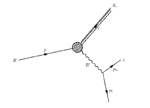
The semileptonic decay of a B meson into a charmed hadronic state and a lepton-neutrino pair.

Much more detailed information on the underlying dynamics of the process can be obtained by analyzing less inclusive observables. These observables can be constructed from the triple differential decay rate for this process,

$$B(p)\to l(p_{l})+\bar{\nu}(p_{\bar{\nu}})+X_{c}(r)\ ,$$ (4.44)

which depends on three different kinematical variables $q^{2},r$ and $E_{l}$, where $q=p_{l}+p_{\nu}$ is the total four momentum of the leptonic system, $r=p-q$ is the four-momentum of the charmed hadronic final state, with invariant mass $r^{2}=M_{X}^{2}$, and $E_{l}$ is the lepton energy in the rest frame of the decaying $b$ quark. This triple differential distribution can be decomposed, using the kinematics of the process and the symmetries of the theory, in terms of three structure functions,

$$\frac{d^{3}\Gamma}{dq^{2}drdE_{l}}(q^{2},r,E_{l})=\frac{G_{F}^{2}|V_{cb}|^{2}}{16\pi^{4}}\Bigg{[}\hat{q}^{2}W_{1}(\hat{q}^{2},\hat{u})-$$

$$\left(2v\hat{p}_{l}-2v\hat{p}_{l}v\hat{q}+\frac{\hat{q}^{2}}{2}\right)W_{2}(\hat{q}^{2},\hat{u})+\hat{q}^{2}\left(2v\hat{p}_{l}-v\hat{q}\right)W_{3}(\hat{q}^{2},\hat{u})\Bigg{]}\ ,$$ (4.45)

where $u^{2}=r^{2}-m_{c}^{2}$, $v=p/m_{b}$ and the quantities with a hat are dimensionless quantities normalized to $m_{b}$. All the structure functions $W_{i}(\hat{q}^{2},\hat{u})$ have both a perturbative expansion in powers of $\alpha_{s}$, and a nonperturbative expansion in powers of $1/m_{b}$, which can be computed in the framework of the heavy quark expansion. For example, the $\mathcal{O}(\alpha_{s})$ corrections for all the differential distributions that can be constructed from Eq. 4.1.3 have become available recently [trott, agru].

Typical observables which are accessible in experiments are convolutions of the differential spectra with suitable weight functions over a large enough range, with kinematical cuts. A particular case of these observables are the moments of differential decay distributions. In this thesis we will study the leptonic moments, defined as

$$L_{n}(E_{0},\mu)\equiv\int_{E_{0}}^{E_{\max}}dE_{l}\left(E_{l}-\mu\right)^{n}\int dq^{2}dr\frac{d^{3}\Gamma}{dq^{2}drdE_{l}}(q^{2},r,E_{l})\ ,$$ (4.46)

where $E_{0}$ is a lower cut on the lepton energy, required experimentally to select this decay mode from the background from other B meson decays, and $E_{\max}$ is the maximum energy allowed from the kinematics of the process that the lepton can have,

$$E_{\max}=\frac{m_{B}^{2}-m_{D}^{2}}{2m_{B}}\ ,$$ (4.47)

where $m_{B}$ is the average of the mass of the neutral and charged B mesons, and similarly for $m_{D}$. In particular we are interested in the behavior of the lepton energy distribution, defined as

$$\frac{d\Gamma}{dE_{l}}(E_{l})\equiv\int dq^{2}dr\frac{d^{3}\Gamma}{dq^{2}drdE_{l}}(q^{2},r,E_{l})\ ,$$ (4.48)

which is related to the observable leptonic moments via

$$L_{n}(E_{0},\mu)=\int_{E_{0}}^{E_{\max}}dE_{l}\left(E_{l}-\mu\right)^{n}\frac{d\Gamma}{dE_{l}}(E_{l})\ .$$ (4.49)

Available published data for this process consist on moments of the lepton spectrum, Eq. 4.49. In Section 6.3 we reconstruct the underlying lepton spectrum, Eq. 4.48, from experimental information on its moments together with additional theoretical constraints, using the general strategy to parametrize experimental data described in Chapter 5.

The lepton energy spectrum Eq. 4.48 in $B\to X_{c}l\nu$ decays can also be expanded in a power series both in $\alpha_{s}$ and in $1/m_{b}$. The leading order spectrum in both expansions is given by [ope2]

$$\frac{d\Gamma}{dy}\left(B\to X_{c}l\nu\right)=\Gamma_{0}2y^{2}\left[(1-f)^{2}(1+2f)(2-y)+(1-f)^{3}(1-y)\right]\theta(1-y-\rho)\ ,$$ (4.50)

where

$$\Gamma_{0}=\frac{G_{F}^{2}m_{b}^{5}}{192\pi^{3}}$$ (4.51)

is the total semileptonic decay rate in the parton model for massless final state quarks and we have defined

$$f=\frac{\rho}{1-y}\ ,\qquad\rho=\frac{m_{c}^{2}}{m_{b}^{2}}\ ,\qquad y=\frac{2E_{l}}{m_{b}}\ .$$ (4.52)

The leading perturbative $\mathcal{O}(\alpha_{s})$ corrections to this spectrum have been known for some time [kuhn], and there are estimations of the size of higher order terms [blm2] though the BLM expansion [blm]. The leading nonperturbative $\mathcal{O}(1/m_{b}^{2})$ corrections to the lepton energy spectrum were computed in Refs. [ope2, manohar] and the $\mathcal{O}(1/m_{b}^{3})$ corrections in Ref. [gremm]. Similar expansions exist also for the lepton energy moments (see Ref. [gambinomom] and references therein), where nonperturbative corrections have been computed up to $\mathcal{O}\left(1/m_{b}^{3}\right)$. Note that nonperturbative effects in the $1/m_{b}$ expansion ara parametrized by B meson expectation values that need to be extracted from experimental data. In Fig. 4.5 we show the lepton energy spectrum as measured from the Babar collaboration [Aubert:2004td], before applying several experimental corrections, and the corresponding leading order theoretical prediction, Eq. 4.50, for different values of the b quark mass.

Figure 4.5:

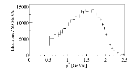
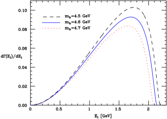
The folded lepton energy spectrum as measured by the Babar collaboration as a function of the lepton momentum (left) and the corresponding leading order theoretical prediction (right).

In Section 6.3 we construct a neural network parametrization of the leptonic spectrum, Eq. 4.48, from all the available experimental information on moments of this spectrum, supplemented by kinematical constraints. This application will show that the neural network approach can be used to reconstruct in a efficient way a function when the only available information comes from moments of this function. As a byproduct of such parametrization, we will provide also a determination of the b quark mass in the $\overline{\mathrm{MS}}$ scheme $\overline{m}_{b}\left(\overline{m}_{b}\right)$.

4.1.4 Hadronic tau decays

The hadronic decays of the tau lepton [tsai, tauthesis] are for a variety of reasons a key process to study both the perturbative and non perturbative regimes of Quantum Chromodynamics [pich, diberder]. Its importance for precision studies of hadronic physics has been extensively studied [physicsaleph], specially thanks to the high quality data provided by the LEP accelerator at CERN [hadrlep1, hadrlep2]. Not only the hadronic tau decays provide one of the most precise determinations of the strong coupling $\alpha_{s}\left(M_{\tau}\right)$, but since the tau mass is not so large as compared to $\Lambda_{\mathrm{QCD}}$, the non-perturbative effects, parametrized by vacuum condensates, can be extracted from experimental data in a clean way. In this Section we will briefly review the theoretical foundations of the QCD analysis of hadronic tau decays.

Figure 4.6:

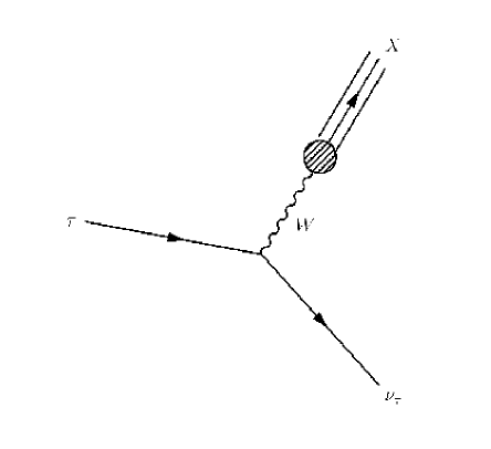
The hadronic decays of the tau lepton. The final state of the decay consists on a hadronic system $X$, composed mainly by pions, and a undetected neutrino.

The hadronic decays of the tau lepton (see Fig. 4.6) are of the form

$$\tau\to X\nu_{\tau}\ ,$$ (4.53)

where $X$ is an hadronic system, composed basically by pions, with vanishing total strangeness. The final hadronic state can be separated into scalar, vector and axial vector contributions, since parity is maximally violated in $\tau$ decays. The hadronic invariant mass-squared $s$ distribution can be measured for each decay channel. These invariant mass distributions $dN_{V/A}/ds$ are related to the so-called spectral functions $\rho_{i}(s)$ by

$$\rho_{V/A}(s)=K_{V/A}(s)\frac{dN_{V/A}(s)}{ds}\ ,$$ (4.54)

for vector (V) and axial-vector (A) final states, and where $K_{i}(s)$ is a purely kinematic factor. In Fig. 4.7 we show the contributions from the different decay modes to the vector and the axial vector spectral functions [physicsaleph].

Figure 4.7:

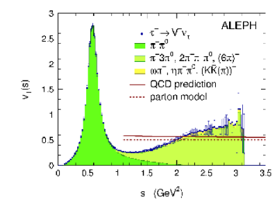
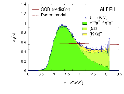
The different contributions to the total vector (left) and axial-vector (right) spectral functions from the hadronic decays of the $\tau$ lepton as measured by the Aleph detector.

Spectral functions are the observables that give access to the inner structure of hadronic tau decays. For reasons to be described in the following, we are in particular interested in the difference between the vector and the axial vector spectral functions,

$$\rho_{V-A}(s)\equiv\rho_{V}(s)-\rho_{A}(s)\ .$$ (4.55)

As spontaneous chiral symmetry breaking is a nonperturbative phenomena, the $\rho_{V/A}(s)$ spectral functions are degenerate in perturbative QCD with massless light quarks, so any difference between vector and axial-vector spectral functions is necessarily generated by non-perturbative dynamics. From perturbative QCD one expects that at some value of $s$ large enough the perturbative result

$$\lim_{s\to\infty}\rho_{V-A}(s)=\rho^{\mathrm{(pert)}}_{V-A}(s)=0\ ,$$ (4.56)

is recovered, but current experimental data do not allow to draw any conclusion of how large $s$ is in reality. Therefore, the spectral function $\rho_{V-A}(s)$ is generated entirely from nonperturbative QCD dynamics, and provides a laboratory for the study of these non-perturbative contributions, which have resulted to be small and therefore difficult to measure in other processes where the perturbative contribution dominates. As will be discussed in brief, these nonperturbative contributions are organized by the Operator product expansion and are parametrized by matrix elements in the vacuum of local operators, the so-called QCD vacuum condensates.

As it is well known [pich], the basis of the comparison of theoretical predictions with experimental data in the hadronic decays of the tau lepton is the fact that unitarity and analyticity connect the spectral functions of hadronic tau decays to the imaginary part of the hadronic vacuum polarization tensor,

$$\Pi_{ij,U}^{\mu\nu}(q)\equiv\int d^{4}x~{}e^{iqx}\left\langle 0|T\left(U^{\mu}_{ij}(x)U^{\nu}_{ij}(0)^{{\dagger}}\right)|0\right\rangle\ ,$$ (4.57)

of vector $U^{\mu}_{ij}\equiv V^{\mu}_{ij}=\bar{q}_{j}\gamma^{\mu}q_{i}$ or axial vector $U^{\mu}_{ij}\equiv A^{\mu}_{ij}=\bar{q}_{j}\gamma^{\mu}\gamma_{5}q_{i}$ color singlet quark currents in corresponding quantum states. After Lorentz decomposition is used to separate the correlation function into its $J=1$ and $J=0$ components,

$$\Pi_{ij,U}^{\mu\nu}(q)=\left(-g^{\mu\nu}q^{2}+q^{\mu}q^{\nu}\right)\Pi^{(1)}_{ij,U}(q^{2})+q^{\mu}q^{\nu}\Pi^{(0)}_{ij,U}(q^{2})\ ,$$ (4.58)

for non-strange quark currents one identifies

$$\mathrm{Im}\Pi^{(1)}_{\bar{u}d,V/A}(s)=\frac{1}{2\pi}\rho_{V/A}(s)\ .$$ (4.59)

Since as we have shown before the spectral functions $\rho_{V/A}(s)$ can be measured experimentally, Eq. 4.59 provides the basis for the comparison between theoretical predictions in the framework of the operator product expansion for the hadronic correlator, Eq. 4.57, and experimental data in terms of spectral functions, Eq. 4.54. This relation then allows us to implement all the technology of QCD vacuum correlation functions to hadronic tau decays.

As has been mentioned before, the basic tool to study in a systematic way the power corrections introduced by nonperturbative dynamics is the operator product expansion. Since the approach of Ref. [svz], the operator product expansion has been used to perform calculations with QCD on the ambivalent energy regions where nonperturbative effects come into play but still perturbative QCD is relevant. In general, the OPE of a two point correlation function $\Pi^{(J)}(s)$ takes the form [pich]

$$\Pi^{(J)}(s)=\sum_{D=0,2,4,\ldots}\frac{1}{(-s)^{D/2}}\sum_{\mathrm{dim}\mathcal{O}=D}C^{(J)}(s,\mu)\left\langle\mathcal{O}(\mu)\right\rangle\ ,$$ (4.60)

where the arbitrary parameter $\mu$ separates the long distance nonperturbative effects absorbed into the vacuum expectation elements $\left\langle\mathcal{O}(\mu)\right\rangle$, from the short distance effects which are included in the Wilson coefficient $C^{(J)}(s,\mu)$, and $J$ is the parity of the correlator. The operator of dimension $D=0$ is the unit operator (the perturbative series) In the case we are interested in, the vector-axial vector correlator, the operator product expansion has no perturbative term and reads

$$\Pi(Q^{2})\Big{|}_{V-A}\equiv\sum_{n=1}^{\infty}\frac{1}{Q^{2n+4}}C_{2n+4}(Q^{2},\mu^{2})\left\langle\overline{\mathcal{O}}_{2n+4}(\mu^{2})\right\rangle\ ,$$ (4.61)

where we observe that the $D=6$ term is the first non-vanishing non-perturbative contribution, in the limit of massless light quarks, to the $\rho_{V-A}(s)$ spectral function and, moreover, it has been shown to be the dominant one. Therefore, this spectral function should provide a source for a clean extraction of the value of the nonperturbative contributions from experimental data.

Even if the $\rho_{V-A}(s)$ spectral function is purely non-perturbative, it has to satisfy several sum rules that can be derived rigorously from QCD. Sum rules have always been an important tool for studies of non-perturbative aspects of QCD, and have been applied to a wide variety of processes, from deep-inelastic scattering, as we have seen in Section 4.1.2, to heavy quark bound states [derafael, srnarison], introduced in Section 4.1.3. Now we will review one of the classical examples of low energy QCD sum rules, the chiral sum rules. The application of chiral symmetry together with the optical theorem leads to low energy sum rules involving the difference of vector and axial vector spectral functions, $\rho_{V-A}(s)$. These sum rules are dispersion relations between real and absorptive parts of a two point correlation function that transforms symmetrically under $SU(2)_{L}\otimes SU(2)_{R}$ in the case of non strange currents. Corresponding integrals are the Das-Mathur-Okubo sum rule [dmo],

$$\frac{1}{4\pi}\int_{0}^{s_{0}\to\infty}ds\frac{1}{s}\rho_{V-A}(s)=\frac{f_{\pi}^{2}\left\langle r_{\pi}^{2}\right\rangle}{3}-F_{A}\ ,$$ (4.62)

where $f_{\pi}$ is the pion decay constant, $\left\langle r_{\pi}^{2}\right\rangle$ the average radius squared of the pion and $F_{A}$ the axial-vector pion form factor, as well as the first and second Weinberg sum rules [weinberg]  ,

$$\frac{1}{4\pi^{2}}\int_{0}^{s_{0}\to\infty}ds\rho_{V-A}(s)=f_{\pi}^{2}\ ,$$ (4.63)

$$\int_{0}^{s_{0}\to\infty}dss\rho_{V-A}(s)=0\ ,$$ (4.64)

where in Eq. 4.63 the right hand side term comes from the integration of the spin zero axial contribution, which for massless non-strange quark currents consists exclusively of the pion pole. Finally, there is the chiral sum rule associated with the electromagnetic splitting of the pion masses [empion],

$$\frac{1}{4\pi^{2}}\int_{0}^{s_{0}\to\infty}dss\ln\frac{s}{\lambda^{2}}\rho_{V-A}(s)=-\frac{4\pi f_{\pi}^{2}}{3\alpha}(m_{\pi^{\pm}}^{2}-m_{\pi^{0}}^{2})\ ,$$ (4.65)

where $\lambda^{2}$ is an arbitrary scale, $\alpha$ the electromagnetic coupling and $m_{\pi}$ the charged and neutral pion masses.

In Section 6.1 we will use our neural network technique to construct a parametrization of the $\rho_{V-A}(s)$ spectral function from experimental data, including all the information on error and correlations, and which incorporates all the constraints from the chiral sum rules and from perturbative QCD. Using this parametrization we will provide a determination of the non-perturbative chiral vacuum condensates, defined in the operator product expansion of Eq. 4.61, whose extraction from experimental data has been the subject of active research in the recent years.

4.2 Global fits of parton distribution functions

As has been discussed in Section 4.1.2, parton distribution functions cannot be computed in perturbation theory, but rather they have to be extracted from experimental data like deep-inelastic scattering. In this Section we review the standard approach to determine parton distributions from experimental data together with their associated uncertainties. In Appendix LABEL:pdfstatus we present a brief overview of the current status of the field of global fits of parton distribution functions.

4.2.1 The standard approach

Let us consider a set of parton distribution functions $q_{i}(x,Q^{2})$, where $i=1,\ldots,2N_{f}+1$, since there is an independent parton distribution for each quark and antiquark flavor, as well as one for the gluon. As we have discussed before, the $Q^{2}$ dependence of the parton distributions is determined by the DGLAP [gl, ap, dok] evolution equations, Eqns. 4.28 and 4.31, so one needs to parametrize and determine from data only the $x$ dependence of the parton distributions at an initial evolution scale $Q_{0}^{2}$. In the standard approach, parton distributions are parametrized with relatively simple functional forms, that in full generality can be taken to be

$$q_{i}(x,Q_{0}^{2})=A_{i}x^{b_{i}}(1-x)^{c_{i}}P_{i}\left(x,d_{i},e_{i},\ldots\right)\ ,\qquad i=1,\ldots,2N_{f}+1\ .$$ (4.66)

The rationale for this functional form is that parton distributions parametrized this way follow quark counting rules [brodsky] at large $x$ and Regge behavior [regge] at small $x$, and $P_{i}(x)$ is a smooth polynomial in $x$ that interpolates between the small-x and the large-x regions. Note that neither of the two limiting behavior (large-x and small-x) of the parton distributions can be derived in a rigorous way from Quantum Chromodynamics, so they are more phenomenological expectations rather that firm theoretical predictions.

In principle one should parametrize and extract from experimental data the $2N_{f}+1$ independent parton distributions. In practice, however, one has to take some assumptions since available data cannot constrain all of them. For example, since there is scarce experimental information of the valence strange distribution $s-\overline{s}$, it is typically set to be zero, $s=\overline{s}$. Another example of this kind of simplifications was the assumption that the sea $\bar{u}$ and $\bar{d}$ distributions were the same. As more and better data becomes available, some of this assumptions are shown not to be true, and one has to allow more freedom in the parametrizations of the parton distributions. For example, the NMC measurements of the Gottfried sum rule (see [fortegottfried] and references therein) showed that for the proton $\bar{u}(x,Q^{2})\neq\bar{d}(x,Q^{2})$. Since that measurement, the assumption $\bar{u}=\bar{d}$ was not used anymore in global fits of parton distributions.

To be definite, we show now the explicit parametrizations from a recent global analysis of parton distributions [mrst_02] from the MRST collaboration. The up and down valence distributions are parametrized as

$$xu_{V}(x,Q_{0}^{2})\equiv x\left(u-\overline{u}\right)(x,Q_{0}^{2})=A_{u}x^{b_{u}}(1-x)^{c_{u}}\left(1+d_{u}\sqrt{x}+e_{u}x\right)\ ,$$ (4.67)

$$xd_{V}(x,Q_{0}^{2})\equiv x\left(d-\overline{d}\right)(x,Q_{0}^{2})=A_{d}x^{b_{d}}(1-x)^{c_{d}}\left(1+d_{d}\sqrt{x}+e_{d}x\right)\ ,$$ (4.68)

then the sea combination of parton distributions is given by

$$xS(x,Q_{0}^{2})=A_{s}x^{b_{s}}(1-x)^{c_{s}}\left(1+d_{s}\sqrt{x}+e_{s}x\right)\ ,$$ (4.69)

where the sea parton distribution is defined as

$$xS(x,Q_{0}^{2})\equiv 2x\left(\overline{u}+\overline{d}+\overline{s}\right)\left(x,Q_{0}^{2}\right)\ ,$$ (4.70)

and the gluon parton distribution is given by

$$xg(x,Q_{0}^{2})=A_{g}x^{b_{g}}(1-x)^{c_{g}}\left(1+d_{g}\sqrt{x}+e_{g}x\right)-F_{g}x^{g_{g}}(1-x)^{h_{g}}\ .$$ (4.71)

Finally, the structure of the light quark sea is taken to be

$$2\overline{u}\ ,\quad 2\overline{d}\ ,\quad 2\overline{s}=0.4S+\Delta\ ,\quad 0.4S-\Delta\ ,\quad 0.2S\ ,$$ (4.72)

$$x\Delta(x,Q_{0}^{2})=x\left(\overline{d}-\overline{u}\right)\left(x,Q_{0}^{2}\right)=A_{\Delta}x^{b_{\Delta}}(1-x)^{c_{\Delta}}\left(1+c_{\Delta}x+d_{\Delta}x^{2}\right)\ .$$ (4.73)

Note that the assumption of a vanishing strange valence distribution $s=\overline{s}$ is also used. Not all the parameters in the above equations are left free, in particular some of them are fixed by quark number conservation sum rules,

$$\int_{0}^{1}u_{V}(x,Q_{0}^{2})=2,\qquad\int_{0}^{1}d_{V}(x,Q_{0}^{2})=1\ .$$ (4.74)

The total number of fitted parameters in this case is around 20. With the above relatively simple parametrization one can describe a wealth of hard-scattering processes, thus showing that QCD factorization [factorization] holds in the majority of high energy processes involving strongly interacting particles.

Note that Ref. [mrst_02] allows for the gluon parton distribution to become negative, as can be seen from Eq. 4.71. This would appear to be in conflict with the interpretation of parton distributions as the probability distributions of the momentum that quarks and gluon carry inside the proton. However, it has been emphasized [fortepos] that parton distributions are not physical quantities, in particular beyond the leading order approximation they depend on the renormalization scheme. Physical quantities, on the other hand, like cross sections and structure functions, satisfy positivity bounds, that is, even if parton distributions are allowed to become negative, structure functions are not since they are observable quantities and therefore are positive definite.

The next step of the global fitting approach is to evolve the set of parton distributions that have been parametrized, Eq. 4.66 at the initial evolution scale $Q_{0}^{2}$, to the scale $Q^{2}$ where there is experimental data using the solution of the DGLAP evolution equations, Eqns. 4.28 and 4.31. Then for each specific process one adds the contribution from the perturbative coefficient functions to construct the corresponding observable, for example deep-inelastic structure functions, as in Eq. 4.16. The number of hard-scattering processes that are nowadays used to constrain the shapes of the different parton distribution functions is rather large. These include

• Deep-inelastic scattering structure functions, $F_{2}(x,Q^{2})$, $F_{3}(x,Q^{2})$ and $F_{L}(x,Q^{2})$, both in charged lepton and in neutrino DIS,

• The Drell-Yan process, $p\bar{p}\to Xl\bar{l}$ in hadronic collisions,

• Jet production, both in $e^{\pm}p$ collisions and in $p\bar{p}$ collisions,

• Gauge boson production $p\bar{p}\to W(Z)X$,

and other processes like prompt photon production and heavy quark production. In any case, it has to be emphasized that deep-inelastic scattering is and will be in the following years the most important source of information on parton distribution functions, specially the precision structure function measurements of the HERA collider [herarev]. The LHC will not only use extensively parton distributions, but it will also be useful to constrain its shape, since it proves a kinematic region not accessible at available colliders, for example with processes like the differential rapidity distribution of gauge boson production [heralhc].

The final step of a global fit is to minimize a suitable statistical estimator, for example the diagonal statistical error

$$\chi^{2}\left(\{a_{i}\}\right)=\sum_{i=1}^{N_{\mathrm{dat}}}\frac{\left(F_{i}^{(\exp)}-F_{i}^{(\mathrm{QCD})}\left(\{a_{l}\}\right)\right)^{2}}{\sigma_{i,\mathrm{stat}}^{2}}\ .$$ (4.75)

where $F_{i}^{(\exp)}$ is the experimental measurement and $F_{i}^{(\mathrm{QCD})}\left(\{a_{i}\}\right)$ the theoretical prediction as a function of the parameters $\{a_{i}\}$ that describe the set of parton distributions. These parameters are determined by the condition that the statistical estimator is minimized, that is, one wants to determine the set of parameters $\{a_{i}^{(0)}\}$ that satisfy the condition

$$\chi^{2}\left(a_{l}^{(0)}\right)\equiv\mathrm{min}_{\{a_{l}\}}\left[\chi^{2}\left(\{a_{l}\}\right)\right]\ .$$ (4.76)

Until some years ago, in global fits of parton distribution functions the error function to be minimized was the statistical error function, Eq. 4.75, where $\sigma_{i,\mathrm{stat}}$ is the total uncorrelated statistical uncertainty. However the precision of modern experimental data made compulsory to consider the effects of the correlated systematic uncertainties. This was so both because the statistical accuracy of the data became higher and the experimental groups became to provide the contributions from the different sources of systematic errors with the experimental data. The inclusion of correlated systematics can be done with two equivalent definitions of the error function $\chi^{2}$. The first one uses the explicit form of the experimental covariance matrix,

$$\chi^{2}=\frac{1}{N_{\mathrm{dat}}}\sum_{i,j=1}^{N_{\mathrm{dat}}}\left(F_{i}^{(\exp)}-F_{i}^{(\mathrm{QCD})}\right)(\mathrm{cov}^{-1})_{ij}\left(F_{j}^{(\exp)}-F_{j}^{(\mathrm{QCD})}\right)\ ,$$ (4.77)

where the covariance matrix of the experimental data is defined as

$$\mathrm{cov}_{ij}=\rho_{ij}\sigma_{\mathrm{tot},i}\sigma_{\mathrm{tot},j}\ ,$$ (4.78)

where $\rho_{ij}$ is the correlation matrix of experimental data and $\sigma_{\mathrm{tot},j}=\sqrt{\sigma^{2}_{\mathrm{stat},j}+\sigma^{2}_{\mathrm{sys},j}}$ is the total experimental uncertainty. Since the number of data points is typically large, the inversion of the covariance matrix might lead to numerical instabilities. For this reason, a equivalent form of Eq. 4.77 was proposed that does not involve explicitely the covariance matrix. This second equivalent definition is given by

$$\chi^{2}=\frac{1}{N_{\mathrm{dat}}}\sum_{i=1}^{N_{\mathrm{dat}}}\frac{1}{\sigma_{\mathrm{stat},i}^{2}}\left(F_{i}^{(\exp)}-F_{i}^{(\mathrm{QCD})}-\sum_{k=1}^{K}r_{k}\beta_{ki}\right)^{2}+\sum_{k=1}^{K}r_{k}^{2}\ ,$$ (4.79)

where $\beta_{ki}$ is the contribution from the $K$ sources of correlated systematic uncertainties. In this approach one has to minimize this $\chi^{2}$ both with respect to the parameters $r_{k}$, which determine the effect of correlated systematics, as well as with respect to the parameters $\{a_{i}\}$ defining the QCD model $F^{(\mathrm{QCD})}$. The problem with this definition is that the number of correlated systematics can be very large, which leads to a formidable minimization task. A way to overcome this difficulty is to perform the minimization with respect to the parameters $r_{k}$ analytically. In this case one obtains a simplified expression,

$$\chi^{2}(\{a_{l}\})=\frac{1}{N_{\mathrm{dat}}}\sum_{i=1}^{N_{\mathrm{dat}}}\frac{\left(F_{i}^{(\exp)}-F_{i}^{(\mathrm{QCD})}\right)^{2}}{\sigma_{i,\mathrm{stat}}^{2}}-\sum_{k,k^{\prime}}^{K}B_{k}(A^{-1})_{kk^{\prime}}B_{k^{\prime}}\ ,$$ (4.80)

where we have defined

$$r_{k}(\{a_{l}\})=\sum_{k^{\prime}=1}^{K}(A^{-1})_{kk^{\prime}}B_{k^{\prime}}\ ,$$ (4.81)

$$B_{k}(\{a_{l}\})=\sum_{i=1}^{N_{\mathrm{dat}}}\frac{\beta_{ki}\left(F_{i}^{(\exp)}-F_{i}^{(\mathrm{QCD})}\right)}{\sigma_{\mathrm{stat},i}^{2}},\quad A_{kk^{\prime}}=\delta_{kk^{\prime}}+\sum_{i=1}^{N_{\mathrm{dat}}}\frac{\beta_{ki}\beta_{k^{\prime}i}}{\sigma_{\mathrm{stat},i}^{2}}\ .$$ (4.82)

Assuming that the measurements $F_{i}^{(\exp)},\sigma_{\mathrm{stat},i}$ and $\beta_{ik}$ are in accord with normal statistics, the $\chi^{2}$ function defined in Eq. 4.80 should have the standard probabilistic interpretation. One can check explicitely that the two definitions are completely equivalent. The advantages and drawbacks of the two approaches in fits with covariance matrix error have been discussed in other contexts, like global fits of neutrino oscillations [fogli]. The main advantage of Eq. 4.79 is that it does not require the inversion of a covariance matrix.

In Fig. 4.8 we show the result of a recent benchmark [heralhc] QCD analysis of parton distribution functions. These results show the characteristic features of the different parton distributions: while the valence distributions have to vanish at small-x, due to quark number conservation, the gluon distribution grows very fast at small-x. The size of this growth depends on whether or not the parametrization of the gluon parton distribution at the initial evolution scale $Q_{0}^{2}$ is singular at $x=0$. The error bands for the parton distributions are computed using some of the techniques discussed in the next Section.

Figure 4.8:

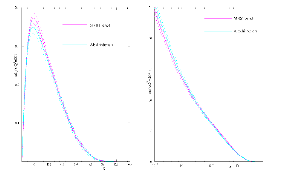
The benchmark parton distribution functions with associated uncertainties as described in Ref. [heralhc]: the valence down distribution (left) and the gluon distribution (right).

During some time it was though that the determination of the best-fit parton distributions were enough for practical phenomenological purposes. However, as better quality data became available, together with the progress in higher-order computations, it was realized that it was necessary to estimate in addition the uncertainties associated to the parton distributions. These uncertainties are of two classes: experimental uncertainties (since parton distributions are extracted from experimental data with errors) and theoretical uncertainties (for example the model dependence in the assumed shapes of the parton distributions, or the possible effects of non-standard evolution at low $x$ [fortelowx]). In the next Section we will review some of the standard methods used to estimate the uncertainties of the parton distributions coming from experimental data errors [pdferrors]. Theoretical uncertainties (see for example [mrst_th]) are rather more complicated to estimate, and we will not review their treatment here. This is so because theoretical errors are not gaussian, and the best one can do to estimate their effects is to provide some suitable prescriptions, but no rigorous statistical analysis is available for these type of uncertainties.

4.2.2 Uncertainties in parton distributions

The first method to estimate the effects of the experimental uncertainties in the parton distributions is called the Offset method [botje], which has mostly been used by the QCD analysis of the ZEUS and H1 collaborations. In this method the systematic uncertainty parameters $r_{k}$ in Eq. 4.79 are fixed to zero in the central fit so that the fitted parameters are as close as possible to the central values of published data. Then they are taken into account for the error analysis. This is done in the following way: in addition to the usual Hessian matrix,

$$H_{ij}=\frac{\partial^{2}\chi^{2}\left(\{a_{m}\},\{r_{n}\}\right)}{\partial a_{i}\partial a_{j}}\ ,$$ (4.83)

defined with respect to the set of parameters $\{a_{l}\}$ defining the QCD model, a second Hessian matrix is defined as

$$V_{jk}=\frac{\partial^{2}\chi^{2}\left(\{a_{m}\},\{r_{n}\}\right)}{\partial a_{j}\partial r_{k}}\ ,$$ (4.84)

which contains information on the variations of the error function $\chi^{2}$ with respect to the systematic uncertainties parametrized by the $r_{k}$ parameters. Then the covariance matrix for the systematic uncertainties is given by

$$C^{\mathrm{sys}}=H^{-1}VV^{T}H^{-1}\ ,$$ (4.85)

and the total covariance matrix is constructed as the sum from the two contributions, the statistical and the systematic,

$$C^{\mathrm{tot}}=C^{\mathrm{stat}}+C^{\mathrm{sys}}\ ,$$ (4.86)

where $C^{\mathrm{stat}}=H^{-1}$ is the standard statistical covariance matrix. In this method the uncertainty in any quantity that depends on the parton distribution functions, $\mathcal{F}\left[\{q_{i}\}\right]$ is computed from

$$\left(\Delta\mathcal{F}\right)^{2}=\sum_{i,j=1}^{N_{\mathrm{par}}}\frac{\partial\mathcal{F}}{\partial a_{i}}C_{ij}\frac{\partial\mathcal{F}}{\partial a_{j}}\ ,$$ (4.87)

by substituting $C$ by the appropriate covariance matrices, $C^{\mathrm{stat}},C^{\mathrm{sys}}$ and $C^{\mathrm{tot}}$ to obtain the total statistical, correlated systematic and total experimental error band respectively. $N_{\mathrm{par}}$ is the total number of parameters used in the parametrization of the set of parton distributions at the starting evolution scale, Eq. 4.66. This method is not statistically rigorous, but it has the virtue that it does not assume gaussianly distributed systematic uncertainties. It gives a conservative error estimate as compared with other methods, like for example the Hessian method with $\Delta\chi^{2}=1$ rule, to be discussed in brief. This method suffers two serious drawbacks: first of all it assumes that linear error propagation gives a decent estimate of the total error propagation, an assumption that has been shown to be not correct in many cases. Second, as can be seen from the above formulae, the estimation of the uncertainties depends heavily on the functional form model than one has assumed for the set of parton distributions.

Another popular method is the so-called Hessian method. In the Hessian method [hessian] one assumes that the deviation in $\chi^{2}$ for the global fit from the minimum value is quadratic in the deviation of the parameters specifying the input parton distributions $\{a_{i}\}$ from their values at the minimum $\{a_{i}^{0}\}$. First one determines the best fit set of parton distributions from the minimization of Eq. 4.79, that is, including the contribution from correlated systematic uncertainties, as opposed to the Offset method. Then to estimate the associated uncertainty one can write

$$\Delta\chi^{2}\equiv\chi^{2}-\chi_{0}^{2}=\sum_{i=1}^{n}\sum_{j=1}^{n}H_{ij}\left(a_{i}-a_{i}^{0}\right)\left(a_{i}-a_{j}^{0}\right)\ ,$$ (4.88)

where $H$ is the Hessian matrix, defined in Eq. 4.83. Standard linear propagation implies that the error on an observable $\mathcal{F}\left[\{q_{i}\}\right]$ is given by

$$\left(\Delta\mathcal{F}\right)^{2}=\Delta\chi^{2}\sum_{i,j=1}^{N_{\mathrm{par}}}\frac{\partial\mathcal{F}}{\partial a_{i}}C_{ij}^{\mathrm{stat}}(\{a_{m}\})\frac{\partial\mathcal{F}}{\partial a_{j}}\ ,$$ (4.89)

where the covariance matrix of the parameters $C^{\mathrm{stat}}$ is again the inverse of the Hessian matrix, Eq. 4.83, and $\Delta\chi^{2}$ is the allowed variation in $\chi^{2}$. Textbook statistics imply that one should have $\Delta\chi^{2}=1$, however it has been argued that a higher value, $\Delta\chi^{2}=100$ is required in order to estimate the uncertainties in a faithful way, due to the fact that data from different experiments is sometimes incompatible [incon].

For practical purposes, it is more numerically stable to diagonalize the covariance matrix and work in the basis of eigenvectors, defined by

$$\sum_{j=1}^{N_{\mathrm{par}}}H_{ij}\left(\{a_{l}\}\right)v_{jk}=\lambda_{k}v_{ik}\qquad i,k=1,\ldots,N_{\mathrm{par}}\ .$$ (4.90)

One has to take into account that since variations in some directions in the parameter space lead to deterioration of the quality of the fit far more quickly than others, the eigenvalues $\lambda_{k}$ span several orders of magnitude. In the Hessian method, one ends up with a set of $2N_{\mathrm{par}}$ sets of parton distributions $S_{i}^{\pm}$. One can therefore propagate the uncertainty associated to the parton distributions to any given observable $\mathcal{F}\left[\{q_{i}\}\right]$ with the following master formula, equivalent to Eq. 4.89,

$$\left(\Delta\mathcal{F}\right)^{2}=\frac{1}{2}\left(\sum_{i=1}^{N_{\mathrm{par}}}\left[\mathcal{F}(\{S_{i}^{+}\})-\mathcal{F}(\{S_{i}^{-}\})\right]^{2}\right)\ .$$ (4.91)

The drawbacks of this method are similar to those of the Offset method: first of all one assumes that the linearized approximation in error propagation is valid, and second errors estimated with this method depend heavily on the functional form choosen for the parametrization of parton distributions. Finally the introduction of non-standard tolerance criteria $\Delta\chi^{2}\ >1$ does not allow to give a statistically rigorous meaning to the resulting uncertainties.

Figure 4.9:

Relative errors of parton distributions in the recent CTEQ6 analysis [cteq6]: up quark parton distribution (left) and gluon parton distribution (right).

The final technique that will be discussed is the Lagrange multiplier method [lagrange], which overcomes some of the drawbacks of the above methods, specially the linearized approximations. To investigate the allowed variation of a specific physical observable is more rigorous using this method that the previously discussed ones. In the Lagrange multiplier approach, one performs a global fit while constraining the values of a physical quantity $\mathcal{F}\left[\{q_{i}\}\right]$ in the neighborhood of their values $\mathcal{F}^{(0)}$ obtained in the unconstrained global fit. The starting point is the best-fit set of parton distributions $S_{0}$ characterized by the parameters $\{a_{i}^{(0)}\}$. The uncertainty associated to the observable $\mathcal{F}$ is estimated in two steps. First we use the Lagrange multiplier method to determine how the minimum of $\chi^{2}\left(\{a_{i}\}\right)$ increases, as $\mathcal{F}$ deviates from the best estimate $\mathcal{F}^{(0)}$, and then one determines the appropriate tolerance of $\chi^{2}\left(\{a_{i}\}\right)$, $\Delta\chi^{2}$. The first step is then minimizing the constrained error function

$$\Psi\left(\lambda,\{a_{i}\}\right)=\chi^{2}\left(\{a_{i}\}\right)+\lambda\mathcal{F}\left(\{a_{i}\}\right)\ ,$$ (4.92)

for various values of $\lambda$, following the chain

$$\lambda_{\alpha}\to\mathrm{min}\left[\Psi\left(\lambda_{\alpha},\{a_{i}\}\right)\right]\to\{a_{i}\left(\lambda_{\alpha}\right)\}\to\mathcal{F}_{\alpha},\chi^{2}_{\alpha}.$$ (4.93)

This procedure generates a parametric relationship between $\chi^{2}$ and the observable, $\mathcal{F}$, in terms of the parameter $\lambda$, so that given an allowed value of $\Delta\chi^{2}$, it is straightforward to derive an allowed range for the observable $\Delta\mathcal{F}$, without any linearized approximation. In practice this procedure generates a sample of sets of parton distributions $\{S_{n}\}$ equal to the size of the parton distribution set parameter space $N_{\mathrm{par}}$, since the minimization is performed in each direction of the parameter space, which are then used to assess the range of variation of $\mathcal{F}$ allowed by the data, using Eq. 4.89.

Figure 4.10:

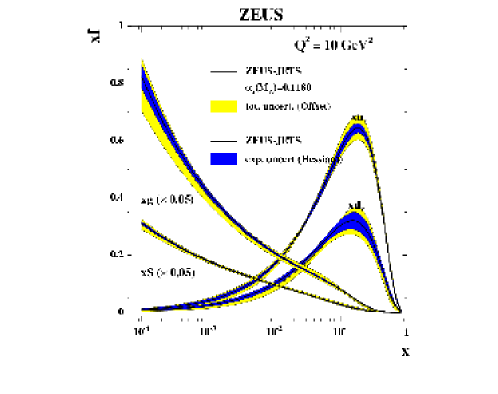
Set of parton distributions with uncertainties computed with different methods from a recent QCD analysis of the ZEUS collaboration [pdfzeus].

It is clear that the Lagrange multiplier method provides a sample of parton distribution sets tailored to assess the uncertainty associated to the physical problem at hand. This procedure does not involve some of the approximations involved in the Hessian and Offset methods, but it still has the problem of the introduction of non-standard tolerance criteria. However, this method suffers from a large practical disadvantage, which is that the global fits of parton distributions must be repeated every time one needs to determine the uncertainties of a different observable coming from parton distributions.

In Figs. 4.9 and 4.10 we show the errors associated to different parton distributions from two different QCD global analysis. Note that the gluon parton distribution in particular has a rather large uncertainty, specially at large and small $x$, where there are no direct constrains from experimental data on its shape. The valence parton distributions, on the other hand, are known with higher accuracy since they are directly constrained from the precise deep-inelastic scattering data.

It must be emphasized that whatever method is used, nowadays there is a common format to represent the uncertainties in parton distribution. This is accomplished by providing, on top of the best-fit parton distribution set, additional sets of error parton distributions, that span the parameter space of the parton distributions allowed by the corresponding experimental uncertainties, estimated with some of the methods described above. With the sample of parton distribution sets, one computes the uncertainty in any physical quantity $\mathcal{F}\left[q_{i}\right]$ by means of Eq. 4.91. All the modern sets from different global QCD analysis of parton distribution function, including the error sets, are available through the LHAPDF library [lhapdf].

The standard approach introduced in this section for the determination of unpolarized parton distributions and the associated uncertainties is also used for similar global QCD analysis which involve different types of parton distributions, like polarized parton distributions [stefpol, aacpol, blumpol], which measure the fraction of the total spin of the proton carried by the different partons, or nuclear parton distributions [nuclearpdf1, nuclearpdf2, nuclearpdf3] which measure how parton distributions are modified in nucleus within heavy nuclei with respect to those of the free nucleon. Also for parametrizations of the photon [photonpdf] and pion [pionpdf] parton distributions from experimental data the standard approach is used. However, in all the above cases experimental data is more scarce and with larger uncertainties than in the case of unpolarized structure functions.

In Section 5.1 we will introduce an alternative approach to estimate faithfully the uncertainties associated to a function parametrized from experimental data. This approach (the Monte Carlo approach) can be seen to be equivalent to the more common technique to determine confidence levels based on the $\Delta\chi^{2}=1$ condition, assuming that in the latter case linear error propagation is a good enough approximation. In Appendix LABEL:mcerrequiv we show explicitely this equivalence within a simple model.

Chapter 5 The neural network approach: General strategy

This Chapter constitutes the core of the present thesis: we describe the strategy that will be used to parametrize experimental data in an unbiased way with faithful estimation of the associated uncertainties, using a combination of Monte Carlo techniques and neural networks as unbiased interpolants. This strategy has three main parts. In the first part, one constructs a Monte Carlo sampling of the experimental data for a given observable, which determines the probability measure of this observable over a finite set of data points. Then we use neural networks as basic interpolating tools, to construct a continuous probability density for the observable under consideration. This parametrization strategy has the advantage that it does not require any assumption, rather than continuity, on the functional form of the underlying law fulfilled by the given observable. It also provides a faithful estimation of the uncertainties, which can be then propagated to other quantities without the need of any linearized approximation. Finally the third step consists on the statistical validation of the constructed probability measure in the space of the parametrized function by means of suitable statistical estimators. In summary, in this Chapter we will describe how given a measured observable $F$, the associated probability measure in the space of functions, $\mathcal{P}\left[F\right]$, can be constructed, so that expectation values of arbitrary functionals of $F$, $\mathcal{F}[F]$ can be computed as with standard probability distributions, that is

$$\left\langle\mathcal{F}[F]\right\rangle\equiv\int\mathcal{D}F\mathcal{P}\left[F\right]\mathcal{F}[F]\ .$$ (5.1)

In Fig. 5.1 we show a summary of our parametrization strategy for the particular case of the proton structure function.

Figure 5.1:

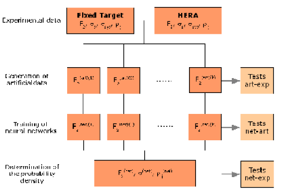
Summary of the strategy presented in this thesis to parametrize experimental data in an unbiased way with faithful estimation of the uncertainties for the particular case of the proton structure function $F_{2}(x,Q^{2})$. As can be seen, the three main steps of our approach are the Monte Carlo generation of replicas of experimental data, the neural network training and finally the statistical validation of the results.

5.1 Monte Carlo sampling of experimental data

In this first Section we describe how we construct a Monte Carlo sample of replicas of the experimental data. We discuss also the statistical estimators which are used to validate the results of the artificial data generation. It has to be emphasized that the Monte Carlo sampling of the data allows to estimate in a faithful way the errors coming from experimental uncertainties associated to the function to be parametrized. Note that this technique to assess the uncertainties in a function is completely independent of the method used to parametrize this function, and in particular it is independent of the fact that we use neural networks. This means that for example this technique could be used in standard fits with polynomial functional forms to determine the associated uncertainties.

5.1.1 Artificial data generation

Let us consider a given observable $F$, which in full generality can be assumed to depend on several kinematical variables $(x_{1},x_{2},x_{3},\ldots)$. If $N_{\mathrm{dat}}$ is the number of experimental measurements of the observable $F$, we define the i-th data point as

$$F_{i}^{(\exp)}\equiv F\left(x_{1i},x_{2i},\ldots\right),\qquad i=1,\ldots,N_{\mathrm{dat}}\ .$$ (5.2)

The first step in our approach is to construct the probability measure of the experimental data for these $N_{\mathrm{dat}}$ data points. This is obtained by means of a Monte Carlo sampling of the experimental data in terms of replicas of the original measurements.

There exist two equivalent techniques to generate the replica sample, depending on how the information on the experimental uncertainties is available. In the first situation, information on all the different independent sources of uncertainty (statistical errors, correlated and uncorrelated systematics, and normalization errors) is available. This is the case for experiments like deep-inelastic scattering for which the detectors and the different sources of correlated uncertainties are well understood. In this case the k-th replica of the experimental data $F^{(\mathrm{art})(k)}$ is generated as

$$F_{i}^{(\mathrm{art})(k)}=\left(1+r_{N}^{(k)}\sigma_{N}\right)\left[F_{i}^{(\exp)}+r_{t,i}^{(k)}\sigma_{t,i}+\sum_{j=1}^{N_{\mathrm{sys}}}r^{(k)}_{\mathrm{sys},j}\sigma_{\mathrm{sys},ji}\right],\quad i=1,\ldots,N_{\mathrm{dat}},\quad k=1,\ldots,N_{\mathrm{rep}}\ .$$ (5.3)

Let us describe the different elements of the above equation. $N_{\mathrm{rep}}$ is the number of Monte Carlo replicas that needs to be generated, while $F_{i}^{(\exp)}$ are the $N_{\mathrm{dat}}$ experimental values of the observable considered. The total uncorrelated uncertainty is defined as

$$\sigma_{t,i}^{2}=\sigma_{\mathrm{stat},i}^{2}+\sum_{j=1}^{N_{u}}\widetilde{\sigma}_{\mathrm{sys},ji}^{2}\ ,$$ (5.4)

as the quadratic sum of the statistical uncertainty $\sigma_{\mathrm{stat},i}$ and the $N_{u}$ uncorrelated systematic uncertainties $\widetilde{\sigma}_{\mathrm{sys},ji}$. The contribution to the i-th data point from the j-th source of correlated systematic uncertainty is denoted by $\sigma_{\mathrm{sys},ji}$, and $\sigma_{N}$ is the total normalization uncertainty. Finally $r_{N}^{(k)},r_{t,i}^{(k)}$ and $r_{\mathrm{sys},j}^{(k)}$ are zero mean univariate gaussian random numbers with the same correlation as the corresponding uncertainties. For example, within a given experiment, for all the data points of the k-th replica we use the same random number for normalization uncertainties, $r_{N}^{(k)}$, since this uncertainty is correlated among all these measurements. The condition that these random numbers are gaussianly distributed implies that

$$\lim_{N_{\mathrm{rep}}\to\infty}\left\langle r_{i}^{(k)}\right\rangle_{\mathrm{rep}}=\mathcal{O}\left(\frac{1}{N_{\mathrm{rep}}}\right)\ ,\qquad\lim_{N_{\mathrm{rep}}\to\infty}\left\langle r_{i}^{(k)2}\right\rangle_{\mathrm{rep}}=1+\mathcal{O}\left(\frac{1}{N_{\mathrm{rep}}}\right)\ .$$ (5.5)

The covariance matrix is constructed from this experimental information as

$${\rm cov}_{ij}=\left(\sum_{k=1}^{N_{\mathrm{sys}}}\sigma_{\mathrm{sys},ki}\sigma_{\mathrm{sys},kj}+F^{(\exp)}_{i}F^{(\exp)}_{j}\sigma_{N}^{2}\right)+\delta_{ij}\sigma^{2}_{t,i}\ ,$$ (5.6)

and the correlation matrix is then given by

$$\rho_{ij}=\frac{{\rm cov}_{ij}}{\sigma_{\mathrm{tot},i}\sigma_{\mathrm{tot},j}}\ ,$$ (5.7)

where the total error $\sigma_{\mathrm{tot},i}$ for the i-th point is given by

$$\sigma_{\mathrm{tot},i}=\sqrt{\sigma_{t,i}^{2}+\sigma_{\mathrm{sys},i}^{2}+\left(F_{i}^{(\exp)}\right)^{2}\sigma_{N}^{2}}\ ,$$ (5.8)

and finally the total correlated uncertainty $\sigma_{\mathrm{sys},i}$ is the sum of all correlated systematics,

$$\sigma_{\mathrm{sys},i}^{2}=\sum_{j=1}^{N_{\mathrm{sys}}}\sigma_{\mathrm{sys},ji}^{2}\ .$$ (5.9)

The presence of correlated systematic uncertainties which are not symmetric for some experiments deserves further comment. As it is well known [barlow1, barlow2, dagostini, dagostini1], asymmetric errors cannot be combined in a simple multi-gaussian framework, and in particular they cannot be added to gaussian errors in quadrature. For the treatment of asymmetric uncertainties, we will follow the approach of Refs. [dagostini, dagostini1], which, on top of several theoretical advantages, is closest to the ZEUS error analysis and thus adequate for a faithful reproduction of the ZEUS data on deep-inelastic structure functions, that is were these asymmetric uncertainties appear. In this approach, a data point with central value $x_{0}$ and left and right asymmetric uncertainties $\sigma_{R}$ and $\sigma_{L}$ (not necessarily positive) is described by a symmetric gaussian distribution, centered at

$$\left\langle x\right\rangle=x_{0}+\frac{\sigma_{R}-\sigma_{L}}{2}\ ,$$ (5.10)

and with width

$$\sigma_{x}^{2}=\Delta^{2}=\left(\frac{\sigma_{R}+\sigma_{L}}{2}\right)^{2}.$$ (5.11)

The ensuing distribution can then be treated in the standard gaussian way.

Once the sampling of the experimental data in terms of a set of replicas of artificial data has been generated, it defines the probability measure of the observable $F$ in those data points where there exist experimental measurements. From this probability density one can compute any estimator as with standard probability distributions. That is, if $\mathcal{A}\left[F\right]$ is any functional of the observable $F$ (the simplest example is the observable itself for the i-th data point, $\mathcal{A}\left[F\right]=F_{i}$ ) then its average as computed from the probability measure is given by

$$\left\langle A^{(\mathrm{art})}\right\rangle_{\mathrm{rep}}\equiv\frac{1}{N_{\mathrm{dat}}}\sum_{k=1}^{N_{\mathrm{rep}}}A^{(\mathrm{art})(k)}\ .$$ (5.12)

Experimental data on the observable $F$ might be available without information on the separation of the different sources of systematic uncertainties, which are then in general collected together in the correlation matrix $\rho_{ij}^{(\exp)}$ of the experimental data. In this second case, the equivalent of Eq. 5.3 is given by

$$F_{i}^{(\mathrm{art})(k)}=F_{i}^{(\exp)}+r_{i}^{(k)}\sigma_{\mathrm{tot},i}\ ,$$ (5.13)

where $\{r_{i}^{(k)}\}$ are gaussianly distributed random numbers with the same correlation as the experimental data points, that is, they verify

$$\frac{\left\langle r_{i}^{(k)}r_{j}^{(k)}\right\rangle_{\mathrm{rep}}-\left\langle r_{i}^{(k)}\right\rangle_{\mathrm{rep}}\left\langle r_{j}^{(k)}\right\rangle_{\mathrm{rep}}}{\sqrt{\left\langle r_{i}^{(k)2}\right\rangle_{\mathrm{rep}}-\left\langle r_{i}^{(k)}\right\rangle^{2}_{\mathrm{rep}}}\sqrt{\left\langle r_{j}^{(k)2}\right\rangle_{\mathrm{rep}}-\left\langle r_{j}^{(k)}\right\rangle^{2}_{\mathrm{rep}}}}=\left\langle r_{i}^{(k)}r_{j}^{(k)}\right\rangle_{\mathrm{rep}}+\mathcal{O}\left(\frac{1}{N_{\mathrm{rep}}}\right)=\rho_{ij}^{(\exp)}\ ,$$ (5.14)

where averages over replicas have been defined in Eq. 5.12. In this situation the covariance matrix can be computed using

$${\rm cov}_{ij}=\rho_{ij}\sigma_{\mathrm{tot},i}\sigma_{\mathrm{tot},j}\ .$$ (5.15)

The number of replicas of the experimental data $N_{\mathrm{dat}}$ that needs to be generated with any of the two equivalent approaches described above is determined by the condition that the Monte Carlo sample reproduces the central values, errors and correlations of the experimental data. The comparison between experimental data and the Monte Carlo sample can be made quantitative by the use of statistical estimators that will be described in the following Section.

5.1.2 Statistical estimators: generated replicas vs. experimental data

In this Section we describe the statistical estimators that are used to validate the results of the replica generation. Let us recall that the probability measure constructed in the previous section aims to reproduce not only central values but also errors and correlations. Therefore we must also validate how well errors and correlations are reproduce by the replica sample. These estimators are the following:

• Average for each experimental point

  $$\left\langle F_{i}^{(\mathrm{art})}\right\rangle_{\mathrm{rep}}=\frac{1}{N_{\mathrm{rep}}}\sum_{k=1}^{N_{\mathrm{rep}}}F_{i}^{(\mathrm{art})(k)}\ .$$ (5.16)

• Associated variance

  $$\sigma_{i}^{(\mathrm{art})}=\sqrt{\left\langle\left(F_{i}^{(\mathrm{art})}\right)^{2}\right\rangle_{\mathrm{rep}}-\left\langle F_{i}^{(\mathrm{art})}\right\rangle^{2}_{\mathrm{rep}}}\ .$$ (5.17)

• Associated covariance and correlation

  $$\rho_{ij}^{(\mathrm{art})}=\frac{\left\langle F_{i}^{(\mathrm{art})}F_{j}^{(\mathrm{art})}\right\rangle_{\mathrm{rep}}-\left\langle F_{i}^{(\mathrm{art})}\right\rangle_{\mathrm{rep}}\left\langle F_{j}^{(\mathrm{art})}\right\rangle_{\mathrm{rep}}}{\sigma_{i}^{(\mathrm{art})}\sigma_{j}^{(\mathrm{art})}}\ .$$ (5.18)

  $$\mathrm{cov}_{ij}^{(\mathrm{art})}=\rho_{ij}^{(\mathrm{art})}\sigma_{i}^{(\mathrm{art})}\sigma_{j}^{(\mathrm{art})}\ .$$ (5.19)

  The three above quantities provide the estimators of the experimental central values, errors and correlations which one extracts from the sample of experimental data.

• Mean variance and percentage error on central values over the $N_{\mathrm{dat}}$ data points.

  $$\left\langle V\left[\left\langle F^{(\mathrm{art})}\right\rangle_{\mathrm{rep}}\right]\right\rangle_{\mathrm{dat}}=\frac{1}{N_{\mathrm{dat}}}\sum_{i=1}^{N_{\mathrm{dat}}}\left(\left\langle F_{i}^{(\mathrm{art})}\right\rangle_{\mathrm{rep}}-F_{i}^{(\mathrm{exp})}\right)^{2}\ ,$$ (5.20)

  $$\left\langle PE\left[\left\langle F^{(\mathrm{art})}\right\rangle_{\mathrm{rep}}\right]\right\rangle_{\mathrm{dat}}=\frac{1}{N_{\mathrm{dat}}}\sum_{i=1}^{N_{\mathrm{dat}}}\left[\frac{\left\langle F_{i}^{(\mathrm{art})}\right\rangle_{\mathrm{rep}}-F_{i}^{(\mathrm{exp})}}{F_{i}^{(\mathrm{exp})}}\right]\ .$$ (5.21)

  We define analogously $\left\langle V\left[\left\langle\sigma^{(\mathrm{art})}\right\rangle_{\mathrm{rep}}\right]\right\rangle_{\mathrm{dat}}$, $\left\langle V\left[\left\langle\rho^{(\mathrm{art})}\right\rangle_{\mathrm{rep}}\right]\right\rangle_{\mathrm{dat}}$, $\left\langle V\left[\left\langle\mathrm{cov}^{(\mathrm{art})}\right\rangle_{\mathrm{rep}}\right]\right\rangle_{\mathrm{dat}}$,
  and $\left\langle PE\left[\left\langle\sigma^{(\mathrm{art})}\right\rangle_{\mathrm{rep}}\right]\right\rangle_{\mathrm{dat}}$, $\left\langle PE\left[\left\langle\rho^{(\mathrm{art})}\right\rangle_{\mathrm{rep}}\right]\right\rangle_{\mathrm{dat}}$ and $\left\langle PE\left[\left\langle\mathrm{cov}^{(\mathrm{art})}\right\rangle_{\mathrm{rep}}\right]\right\rangle_{\mathrm{dat}}$, for errors, correlations and covariances respectively.

  These estimators indicate how close the averages over generated data are to the experimental values. Note that in averages over correlations and covariances one has to use the fact that correlation and covariances matrices are symmetric matrices, and thus one has to be careful to avoid double counting. For example, the percentage error on the correlation will be defined as

  $$\left\langle PE\left[\left\langle\rho^{(\mathrm{art})}\right\rangle_{\mathrm{rep}}\right]\right\rangle_{\mathrm{dat}}=\frac{2}{N_{\mathrm{dat}}\left(N_{\mathrm{dat}}+1\right)}\sum_{i=1}^{N_{\mathrm{dat}}}\sum_{j=i}^{N_{\mathrm{dat}}}\left[\frac{\left\langle\rho_{ij}^{(\mathrm{art})}\right\rangle_{\mathrm{rep}}-\rho_{ij}^{(\mathrm{exp})}}{\rho_{ij}^{(\mathrm{exp})}}\right]\ ,$$ (5.22)

  and similarly for averages over elements of the covariance matrix.

• Scatter correlation:

  $$r\left[F^{(\mathrm{art})}\right]=\frac{\left\langle F^{(\mathrm{exp})}\left\langle F^{(\mathrm{art})}\right\rangle_{\mathrm{rep}}\right\rangle_{\mathrm{dat}}-\left\langle F^{(\mathrm{exp})}\right\rangle_{\mathrm{dat}}\left\langle\left\langle F^{(\mathrm{art})}\right\rangle_{\mathrm{rep}}\right\rangle_{\mathrm{dat}}}{\sigma_{s}^{(\mathrm{exp})}\sigma_{s}^{(\mathrm{art})}}\ ,$$ (5.23)

  where the scatter variances are defined as

  $$\sigma_{s}^{(\mathrm{exp})}=\sqrt{\left\langle\left(F^{(\exp)}\right)^{2}\right\rangle_{\mathrm{dat}}-\left(\left\langle F^{(\exp)}\right\rangle_{\mathrm{dat}}\right)^{2}}\ ,$$ (5.24)

  $$\sigma_{s}^{(\mathrm{art})}=\sqrt{\left\langle\left(\left\langle F^{(\mathrm{art})}\right\rangle_{\mathrm{rep}}\right)^{2}\right\rangle_{\mathrm{dat}}-\left(\left\langle\left\langle F^{(\mathrm{art})}\right\rangle_{\mathrm{rep}}\right\rangle_{\mathrm{dat}}\right)^{2}}\ .$$ (5.25)

  We define analogously $r\left[\sigma^{(\mathrm{art})}\right]$, $r\left[\rho^{(\mathrm{art})}\right]$ and $r\left[\mathrm{cov}^{(\mathrm{art})}\right]$. Note that the scatter correlation and scatter variance are not related to the variance and correlation Eqns. 5.17-5.19. The scatter correlation indicates the size of the spread of data around a straight line. Specifically $r\left[\sigma^{(\mathrm{art})}\right]=1$ implies that $\left\langle\sigma_{i}^{(\mathrm{art})}\right\rangle$ is proportional to $\sigma_{i}^{(\mathrm{exp})}$.

• Average variance:

  $$\left\langle\sigma^{(\mathrm{art})}\right\rangle_{\mathrm{dat}}=\frac{1}{N_{\mathrm{dat}}}\sum_{i=1}^{N_{\mathrm{dat}}}\sigma_{i}^{(\mathrm{art})}\ .$$ (5.26)

  We define analogously $\left\langle\rho^{(\mathrm{art})}\right\rangle_{\mathrm{dat}}$ and $\left\langle\mathrm{cov}^{(\mathrm{art})}\right\rangle_{\mathrm{dat}}$, as well as the corresponding experimental quantities. This quantities are interesting because even if the scatter correlations $r$ are close to 1 there could still be a systematic bias in the estimators Eqns. 5.17-5.19. This is so since even if all scatter correlations are very close to 1, it could be that some of the Eqns. 5.17-5.19 where sizably smaller than its experimental counterparts, even if being proportional to them.

The typical scaling of the various quantities with the number of generated replicas $N_{\mathrm{rep}}$ follows the standard behavior of gaussian Monte Carlo samples [cowan]. For instance, variances on central values scale as $1/N_{\mathrm{rep}}$, while variances on errors scale as $1/\sqrt{N_{\mathrm{rep}}}$. Also, because

$$V[\rho^{(\mathrm{art})}_{ij}]=\frac{1}{N_{\mathrm{rep}}}\left(1-\left(\rho^{(\exp)}_{ij}\right)^{2}\right)^{2}\ ,$$ (5.27)

as can be checked using Eq. LABEL:varcor in Appendix LABEL:probrev, the estimated correlation fluctuates more for small values of $\rho^{(\exp)}$, and thus the average correlation tends to be larger than the corresponding experimental value.

5.2 Neural networks

5.2.1 Neural networks as unbiased interpolants

Artificial neural networks [nnbook, netrev, nnthesis] provide unbiased robust universal approximants to incomplete or noisy data. An artificial neural network consists of a set of interconnected units (neurons). The activation state $\xi_{i}^{(l)}$ of a neuron is determined as a function of the activation states of the neurons connected to it. Each pair of neurons $(i,j)$ is connected by a synapsis, characterized by a weight $\omega_{ij}$. In this thesis we will consider only multilayer feed-forward Perceptrons. These neural networks are organized in ordered layers whose neurons only receive input from a previous layer. In this case the activation state of a neuron in the (l+1)-th layer is given by

$$\xi^{(l+1)}_{i}=g\left(h^{(l+1)}_{i}\right),\qquad i=1,\ldots,n_{l+1},\qquad l=1,\ldots,L-1\ ,$$ (5.28)

$$h^{(l+1)}_{i}=\sum_{j=1}^{n(l)}\omega_{ij}^{(l)}\xi^{(l)}_{j}+\theta_{i}^{(l+1)}\ ,$$ (5.29)

where $\theta_{i}^{(l)}$ is the activation threshold of the given neuron, $n_{l}$ is the number of neurons in the l-th layer, $L$ is the number of layers that the neural network has, and $g(x)$ is the activation function of the neuron, which we will take to be a sigmoid,

$$g(x)=\frac{1}{1+e^{-x}}\ ,$$ (5.30)

except in the last layer, where we use a linear activation function $g(x)$. This enhances the sensitivity of the neural network, avoiding the saturation of the neurons in the last layer. The fact that the activation function $g(x)$ is non-linear allows the neural network to reproduce nontrivial functions. An schematic diagram of a feed-forward artificial neural network can be seen in Fig. 5.2.

Figure 5.2:

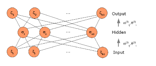
Schematic diagram of a multi-layer feed forward neural network.

Therefore multilayer feed-forward neural networks can be viewed as functions $F:\mathcal{R}^{n_{1}}\to\mathcal{R}^{n_{L}}$ parametrized by weights, thresholds and activation functions,

$$\xi^{L}_{j}=F\left[\xi^{(1)}_{i},\omega_{ij}^{(l)},\theta_{i}^{(l)},g\right],\qquad j=1\ldots,n_{L}\ .$$ (5.31)

It can be proven that any continuous function, no matter how complex, can be represented by a multilayer feed-forward neural network. In particular, it can be shown [nnbook, nnthesis] that two hidden layers suffice for representing an arbitrary complicated function [netref1].

Artificial neural networks are a common tool in experimental particle physics [netrev, netrev2, netrev3] in applications like pattern recognition, where in this context a pattern typically means a experimental measurement as a function of a set of several variables which characterize this event. We are interested in artificial neural networks in order to parametrize physical quantities in an unbiased way, that is, without the need of any assumptions on its functional form behavior. These physical quantities to be parametrized can be either direct experimental measurements (like in the case of deep inelastic structure functions), or they can be related to experimental data through a functional dependence (like in the case of parton distribution functions). Neural networks not only provide universal unbiased interpolants for given physical quantity in the region were there is experimental information, they also have the property that their behavior in extrapolation regions is not determined by their behavior in the data region, as happens in fits with simple functional forms, so they are also useful to assess the uncertainty in extrapolation regions (that is, in regions without information from experimental measurements).

Therefore, the performance of neural networks is worse for extrapolation than for interpolation. That is, new input patterns that are not a mixture of some of the input training patterns cannot be classified in an efficient way in terms of the learnt patterns. In particular, for a feed forward neural network with one hidden layer, the generalization error (that is, the error in the classification of patterns which are very different from the patterns used in the training) is of the order $\mathcal{O}\left(N_{\mathrm{par}}/N_{\mathrm{dat}}\right)$ [netref2], where $N_{\mathrm{par}}$ is the number of neural network parameters and $N_{\mathrm{dat}}$ the number of training patterns.

Another interesting property of artificial neural networks is that they are efficient in combining in an optimal way experimental information from different measurements of the same quantity. That is, when the separation of data points in the space of possible input patterns is smaller than a certain correlation length, the neural network manages to combine the corresponding experimental information, thus leading to a determination of the output pattern (in the present case the function to parametrize) which is more accurate than the individual input patterns (the measurements from the different experiments).

5.2.2 Training strategies

Training a neural network implies the minimization of a suitable statistical estimator. In this Section we discuss the different estimators that are minimized in the neural network training. In the next Section we will analyze the minimization algorithms that are used to implement this training.

For this thesis three different estimators have been used: the central values error function,

$$E_{1}^{(k)}=\frac{1}{N_{\mathrm{dat}}}\sum_{i=1}^{N_{\mathrm{dat}}}\left(F^{(\mathrm{net})(k)}_{i}-F^{(\mathrm{art})(k)}\right)^{2}\ ,$$ (5.32)

the diagonal statistical error function,

$$E_{2}^{(k)}=\frac{1}{N_{\mathrm{dat}}}\sum_{i=1}^{N_{\mathrm{dat}}}\frac{\left(F^{(\mathrm{net})(k)}_{i}-F^{(\mathrm{art})(k)}\right)^{2}}{\sigma_{t,i}^{2}}\ ,$$ (5.33)

where $\sigma_{t,i}$ is the total uncorrelated uncertainty, Eq. 5.4, and finally the error taking into account correlated systematics,

$$E_{3}^{(k)}=\frac{1}{N_{\mathrm{dat}}}\sum_{i,j=1}^{N_{\mathrm{dat}}}\left(F^{(\mathrm{net})(k)}_{i}-F^{(\mathrm{art})(k)}_{i}\right)\left(\left(\overline{\mathrm{cov}}^{(k)}\right)^{-1}\right)_{ij}\left(F^{(\mathrm{net})(k)}_{j}-F^{(\mathrm{art})(k)}_{j}\right)\ ,$$ (5.34)

where in all the above expressions $F^{(\mathrm{net})(k)}_{i}$ is the prediction of the k-th neural network for the i-th data point. Note that in the above equation we have defined the covariance matrix ${\overline{\mathrm{cov}}^{(k)}}_{ij}$ with the normalization uncertainty included as an overall rescaling of the error due to the normalization offset of that replica, namely,

$${\overline{\mathrm{cov}}^{(k)}}_{ij}\equiv\left(\sum_{p=1}^{N_{\mathrm{sys}}}{\overline{\sigma}^{(k)}}_{\mathrm{sys},pi}{\overline{\sigma}^{(k)}}_{\mathrm{sys},pj}\right)+\delta_{ij}{\overline{\sigma}^{(k)}}_{t,i}\ ,$$ (5.35)

with

$$\overline{\sigma}_{a,i}^{(k)}=(1+r^{(k)}_{N}\sigma_{N})\sigma_{a,i}\ ,$$ (5.36)

where $r_{N}^{(k)}$ is the same as in Eq. 5.3. Eq. 5.35 is to be compared with the total covariance matrix, Eq. 5.6. This is necessary in order to avoid a biased treatment of the normalization errors [dagostini]. In Appendix LABEL:toymodel we describe within an explicitely solvable model the effects of an incorrect treatment of normalization uncertainties.

Several relations hold between these estimators. Properties of minimization using the error function defined with the covariance matrix, Eq. 5.34 can be found in Refs. [dagostini, alekhincme]. For example, it can be shown that the following relation holds

$$E_{2}^{(k)}\geq E_{3}^{(k)}\ ,$$ (5.37)

since in the latter case correlated systematic uncertainties are included. The above constraint is useful to cross-check that the experimental covariance matrix Eq. 5.35 has been correctly computed and inverted, without numerical instabilities.

The usefulness of neural networks is due to the availability of a training algorithm. This algorithm allows one to select the values of weights and thresholds such that the neural network reproduces a given set of input-output data, also known as patterns. This procedure is called learning since unlike a standard fitting procedure, there is no need to know in advance the underlying rule which describes the data. In our case the patterns that must be learned are those that minimize any of the estimators described above. Therefore we need to define a suitable minimization strategy to train the neural networks. During the course of this thesis we have used different minimization algorithms, which are described in the following Section.

5.2.3 Minimization algorithms

Three different minimization algorithms have been used during the course of this thesis: back-propagation, genetic algorithms and conjugate gradient, which we now discuss in turn.

• Back-propagation.

  Back-propagation for neural network training was throughly described in Ref. [f2ns] and we summarize its main features here. Back-propagation is a minimization strategy specially suited for the training of neural networks with diagonal error functions. Let us assume that the error function used in the minimization is diagonal and a neural network with a single output layer, then one has

  $$\chi^{2}=\sum_{k=1}^{N_{\mathrm{dat}}}\left(F_{k}^{(\mathrm{net})}-F_{k}^{(\exp)}\right)^{2}\ ,$$ (5.38)

  where $F_{k}^{(\mathrm{net})}$ is the output of the neural network, $F_{k}^{(\mathrm{net})}=\xi^{(L)}_{1}$ when the input of the neural network is $\xi^{(1)}_{l}=x_{lk}$. If the error function is non-diagonal, back-propagation still can be used but the corresponding expressions become more complicated.

  The error function $\chi^{2}$ is a function of the weights and the thresholds of the neural network, and can be minimized by looking for the direction of steepest descent in the space of weights and thresholds, and modifying the parameters in that direction,

  $$\delta\omega_{ij}^{(l)}=-\eta\frac{\partial\chi^{2}}{\partial\omega_{ij}^{(l)}}\ ,$$ (5.39)

  $$\delta\theta_{i}^{(l)}=-\eta\frac{\partial\chi^{2}}{\partial\theta_{i}^{(l)}}\ ,$$

  where $\eta$ is the so-called learning rate. The non-trivial result on which back-propagation training is based is that it can be shown that the steepest descent direction is given by the following recursive expression:

  $$\delta\omega_{ij}^{(l)}=\sum_{k=1}^{N_{\mathrm{dat}}}\Delta_{i}^{(l)k}\xi_{j}^{(l-1)k};\qquad i=1,\ldots,n_{l},\qquad j=1,\ldots,n_{l-1}\ ,$$ (5.40)

  $$\delta\theta_{i}^{(l)}=-\sum_{k=1}^{N_{\mathrm{dat}}}\Delta_{i}^{(l)k},\qquad i=1,\ldots,n_{l}\ ,$$ (5.41)

  where the information on the goodness of the fit is fed to the last layer through

  $$\Delta_{1}^{(L)k}=g^{\prime}\left(h_{i}^{(L)k}\right)\left[F_{k}^{(\mathrm{net})}-F_{k}^{(\exp)}\right]\ ,$$ (5.42)

  where the $h$ function is defined in Eq. 5.29, and then back-propagated to the rest of the network by

  $$\Delta_{i}^{(l-1)k}=g^{\prime}\left(h_{i}^{(L)k}\right)\sum_{j=1}^{n_{l}}\Delta_{j}^{(l)k}\omega_{ij}^{(l)}\ .$$ (5.43)

  The procedure is iterated until a suitable converged criterion is satisfied, as will be described in brief. To avoid getting stuck in local minima, it is useful to add a momentum term in the variations of the parameters. This means that Eq. 5.39 should be replaced by

  $$\delta\omega_{ij}^{(l)}=-\eta\frac{\partial\chi^{2}}{\partial\omega_{ij}^{(l)}}+\alpha\delta\omega_{ij}^{(l)}(\mathrm{last})\ ,$$ (5.44)

  $$\delta\theta_{i}^{(l)}=-\eta\frac{\partial\chi^{2}}{\partial\theta_{i}^{(l)}}+\alpha\delta\theta_{i}^{(l)}(\mathrm{last})\ ,$$

  where (last) indicates the use of the last value of the update for the weights and the thresholds before the current one and $\alpha$ determines the size of the momentum term. The drawbacks of back-propagation minimization is that it is not specially suited for non-linear error functions, or for error functions which depend on the neural network output through convolutions.

  One major improvement of this minimization algorithm during the course of the present thesis was to implement weighted training, in order in increase the efficiency of the algorithm when the experimental data consist on many different experiments. Since weighted training does not depend on the minimization algorithm, we discuss it later in this Section.

• Genetic Algorithms.

  Genetic algorithms are the generic name of function optimization algorithms that do not suffer of the drawbacks that deterministic minimization strategies have when applied to problems with a large parameter space. Genetic algorithms for neural network training were introduced in this context in [condensates], and it is a minimization strategy that has been used in different high energy physics applications [gathesis]. This method is specially suitable for finding the global minima of highly nonlinear problems, as is the one we are facing in this thesis. Genetic algorithms have several advantages with respect to deterministic minimization methods:

  1. They simultaneously work on populations of solutions, rather than tracing the progress of one point through the parameter space. This gives them the advantage of checking many regions of the parameter space at the same time, lowering the possibility that a global minimum gets missed.

  2. No outside knowledge such as local gradient of the minimized function is required.

  3. They have a built-in mix of stochastic elements applied under deterministic rules, which improves their behavior in problems with many local extrema, without the serious performance loss that a purely random search would bring.

  All the power of genetic algorithms lies in the repeated application of three basic operations: mutation, crossover and selection, which we describe in the following. The first step is to encode the information of the parameter space of the function we want to minimize into an ordered chain, called chromosome. If $N_{\mathrm{par}}$ is the size of the parameter space, then a point in this parameter space will be represented by a chromosome,

  $${\bf a}=\left(a_{1},a_{2},a_{3},\ldots,a_{N_{\mathrm{par}}}\right)\ .$$ (5.45)

  In our case each bit $a_{i}$ of a chromosome corresponds to either a weight $\omega^{(l)}_{ij}$ or a threshold $\theta^{(l)}_{i}$ of a neural network. Once we have the parameters of the neural network written as a chromosome, we replicate that chain until we have a number $N_{\mathrm{tot}}$ of chromosomes. Each chromosome has an associated fitness $f$, which is a measure of how close it is to the best possible chromosome (the solution of the minimization problem under consideration). In our case, the fitness of a chromosome is given by the inverse of the function to minimize

  $$f\left({\bf a}\right)=\frac{1}{\chi^{2}\left({\bf a}\right)}\ ,$$ (5.46)

  so chromosomes with larger fitness correspond to those with smaller value of the function to minimize $\chi^{2}$.

  Then we apply the three basic operations:

  • Mutation:

    Select randomly a bit (an element of the chromosome) and mutate it. The size of the mutation is called mutation rate $\eta$, and if the k-th bit has been selected, the mutation is implemented as

    $$a_{k}\to a_{k}+\eta\left(r-\frac{1}{2}\right)\ ,$$ (5.47)

    where $r$ is a uniform random number between 0 and 1. Over the span of several generations, even a stagnated chromosome position can become reactivated by mutation. The optimal size of the mutation rate must be determined for each particular problem, or it can be adjusted dynamically as a function of the number of iterations.

  • Crossover:

    This operation helps in obtaining a child generation which is genetically different from the parents. Crossover means selecting at random pairs of individuals, for each pair determine randomly a crossover bit $s$, and from this crossover point interchange the bits between the two individuals.

  • Selection:

    Once mutations and crossover have been performed into the population of individuals characterized by chromosomes, the selection operation ensures that individuals with best fitness propagate into the next generation of genetic algorithms. Several selection operators can be used. The simplest method is to select simply the $N_{\mathrm{chain}}$ chromosomes, out of the total population of $N_{\mathrm{tot}}$ individuals, with best fitness. Later we will describe a more efficient selection method based on probabilistic selection.

  The procedure is repeated iteratively until a suitable convergence criterion is satisfied. Each iteration of the procedure is called a generation. A general feature of genetic algorithms is that the fitness approaches the optimal value within a relatively small number of generations.

  The theoretical concept behind the success of genetic algorithms is the concept of patterns or schemata within the chromosomes [gabook]. Rather than operating only with $N_{\mathrm{tot}}$ individuals in each generation, a genetic algorithm works with a much higher number of schemata that partly match the actual chromosomes. If for simplicity we consider chromosomes whose elements can take only binary values, the concept of schemata means that a chromosome like 10110 matches $2^{5}$ schemata, such as **11* or 1*1*0. The generalization of this concept to continuous parameters is straightforward. Since fit chromosomes are handled down to the next generation more often than unfit ones, the number of copies of a certain schema S associated with fit chromosomes will increase from one generation to the next,

  $$n_{S}(t+1)=n_{S}(t)\frac{\bar{f}(S)}{\bar{f}_{\mathrm{tot}}}\ ,$$ (5.48)

  where $\bar{f}(S)$ is the average fitness of all individuals whose chromosome match schema S and $\bar{f}_{\mathrm{tot}}$ is the average fitness of all individuals. This implies that if we assume a certain schema approximately giving all matching chromosomes a constant fitness advantage $c$ over the average

  $$\bar{f}(S)\equiv\left(1+c\right)\bar{f}_{\mathrm{tot}}\ ,$$ (5.49)

  one obtains an exponential growth of the number of this schema from one generation to the next,

  $$n_{S}(t)=n_{S}(0)(1+c)^{t}\ .$$ (5.50)

  The above derivation is a rough approximation to the behavior in realistic cases, and it needs to be corrected for effects like mutation. To this purpose we define two measures on schemata:

  1. The defining length $\delta$ is the distance between the furthest two fixed positions. In the above example, the defining length in 1*1*0 is $\delta=4$.

  2. The order $o$ of a shema is the number of fixed positions it contains. In the above example, $o=3$.

  With these measures, if $L$ is the length of a chromosome (that is, the number of parameters $N_{\mathrm{par}}$ of the function we are minimizing) the following bound can be derived

  $$n_{S}(t+1)\geq n_{S}(t)\frac{\bar{f}(S)}{\bar{f}_{\mathrm{tot}}}\left[1-\frac{\delta(S)}{L-1}-o\left(S\right)p_{m}\right]\ .$$ (5.51)

  The first correction includes the effect of crossover and the second implements the effects of mutations, since in a schema of order $o$, there is a probability $\left(1-p_{m}\right)^{o}\sim\left(1-op_{m}\right)$ that the schema survives mutation, where $p_{m}=1/N_{\mathrm{par}}$ is the probability to select a bit at random out out the total $N_{\mathrm{par}}$ bits of a chromosome chain. A consequence of Eq. 5.51 is that short, low-order schemata of high fitness are the building blocks towards a solution of the problem. During a run of the genetic algorithms, the selection operator ensures that building blocks associated with fitter individuals propagate through the population. It can be shown [gabook] that in a population of size $N_{\mathrm{tot}}$, approximately $\mathcal{O}(N^{3}_{\mathrm{tot}})$ schemata are processed in each generation.

  The basic genetic algorithms that we have introduced above can be extended in many ways to address specific problems. Several improvements over this basic version of the algorithm have been implemented in the course of this thesis. The first one is the introduction of multiple mutations $N_{\mathrm{mut}}\geq 2$. This is helpful to avoid local minima, thereby increasing the speed of training. It is crucial that rates for these additional mutations are large, in order to allow for jumps from a local minimum to a deeper one. That is, after the first mutation is performed, additional mutations are performed

  $$a_{l}=a_{l}+\eta_{p}\left(r-\frac{1}{2}\right)\ ,\qquad p=2,\ldots,N_{\mathrm{mut}}\ ,$$ (5.52)

  with mutation rate $\eta_{p}$ and probability $P_{p}$. Each time a new mutation is performed, a different bit $a_{l}$ of the chromosome chain is selected at random.

  Second, we have introduced a probabilistic selection for the mutated chromosome chains, instead of the basic deterministic selection. This is helpful in allowing for mutations which only become beneficial after a combination of several individual mutations, and allows for a more efficient exploration of the whole space of minima. Once one has the mutated population of $N_{\mathrm{tot}}$ individuals, instead of selecting the $N_{\mathrm{chain}}$ individuals with smallest $\chi^{2}$, one selects first the chromosome with smallest $\chi^{2}$, with value $\chi^{2}\left({\bf a}_{1}\right)$, and then selects the remaining $N_{\mathrm{chain}}$ individuals according to the probability

  $$P_{i}\left(\chi^{2}\left({\bf a}_{i}\right)\right)=\exp\left(\frac{-\left(\chi^{2}\left({\bf a}_{i}\right)-\chi^{2}\left({\bf a}_{1}\right)\right)}{T}\right)\ ,\qquad i=2,\ldots,N_{\mathrm{tot}}\ ,$$ (5.53)

  where $T$ is the temperature of the system, in analogy with the Metropolis algorithm in Monte Carlo simulations [metropolis]. At high temperatures even the chromosomes with bad fitness have some probability to propagate to the next generation, while at low temperature one recovers the deterministic selection rule. With this selection criteria, individuals with accidentally bad fitness but with relevant schemata can propagate to the next generations. Of course, after a number of generations only the individuals with good fitness will propagate through the generations.

• Conjugate Gradient

  Conjugate gradient minimization exploits in an efficient way the information on both the function to minimize $\chi^{2}\left({\bf a}\right)$ and its gradient, $\nabla\chi^{2}\left({\bf a}\right)$, where as in Eq. 5.45 ${\bf a}$ stands for the set of weights and thresholds that characterize the neural networks. Starting with an arbitrary initial vector, ${\bf g}_{0}$ and letting ${\bf h}_{0}={\bf g}_{0}$, the conjugate gradient method constructs two sequences of vectors from the recurrence

  $${\bf g}_{i+1}={\bf g}_{i}-\lambda_{i}{\bf A}\cdot{\bf h}_{i},\qquad{\bf h}_{i+1}={\bf g}_{i+1}+\gamma_{i}{\bf h}_{i},\qquad i=0,1,2,\ldots$$ (5.54)

  where we have assumed that the function to be minimized can be approximated by a quadratic form

  $$\chi^{2}\left({\bf a}\right)\sim C-{\bf B}\cdot{\bf a}+\frac{1}{2}{\bf a}\cdot{\bf A}\cdot{\bf a}+\mathcal{O}\left(a^{3}\right)\ ,$$ (5.55)

  and the scalars are defined as

  $$\lambda_{i}=\frac{{\bf g}_{i}\cdot{\bf g}_{i}}{{\bf h}_{i}\cdot{\bf A}\cdot{\bf h}_{i}}\ ,$$ (5.56)

  $$\gamma_{i}=\frac{{\bf g}_{i+1}\cdot{\bf g}_{i+1}}{{\bf g}_{i}\cdot{\bf g}_{i}},$$ (5.57)

  and the dimension of each of the above vectors is $N_{\mathrm{par}}$, the size of the parameter space. With these definitions the following orthogonality and conjugacy conditions hold,

  $${\bf g}_{i}\cdot{\bf g}_{j}=0,\qquad{\bf h}_{i}\cdot{\bf A}\cdot{\bf h}_{j}=0,\qquad{\bf g}_{i}\cdot{\bf h}_{j}=0,\qquad j<i\ .$$ (5.58)

  If one knew the Hessian matrix ${\bf A}$ in Eq. 5.56, the conjugate gradient method would take us to the minimum of $\chi^{2}\left({\bf a}\right)$, but in general this Hessian matrix is not available. However, it can be proven the following property: suppose we happen to have ${\bf g}_{i}=-\nabla\chi^{2}\left({\bf a}_{i}\right)$ at some point ${\bf a_{i}}$ of the parameter space. Now we proceed from the point ${\bf a}_{i}$ along the direction ${\bf h}_{i}$ to the local minimum of $\chi^{2}$ located at the point ${\bf a}_{i+1}$ and then set ${\bf g}_{i+1}=-\nabla\chi^{2}\left({\bf a}_{i+1}\right)$. Then the vector ${\bf g}_{i+1}$ constructed this way is the same that the one that would have been constructed from Eq. 5.54 if the Hessian matrix had been known.

  Once we have constructed a set of conjugate directions, the minimization of the function $\chi^{2}\left({\bf a}\right)$ is straightforward: starting from an initial point in the parameter space ${\bf a}_{1}$, one has to find the quantity $\alpha_{k}$ that minimizes

  $$\chi^{2}\left({\bf a}_{k}+\alpha_{k}{\bf g}_{k}\right)$$ (5.59)

  and then one sets

  $${\bf a}_{k+1}={\bf a}_{k}+\alpha_{k}{\bf g}_{k}$$ (5.60)

  and this procedure is repeated from $k=1$ to $k=N_{\mathrm{par}}$. If the function to be minimized was a quadratic form, conjugate gradient minimization would find the minimum in a single iterations. Obviously, for real functions the length of the minimization is typically larger. Conjugate gradient minimization is also a suitable minimization algorithm for nonlinear error functions, and the main reason for its efficiency is the optimal use of the information contained in the gradient of the function to be minimized $\nabla\chi^{2}$.

Once we have described the different minimization algorithms that will be used for neural network training, we discuss the weighted training procedure. The essential idea about weighted training is that during the neural network training some experimental points are given more weight in the error function than others. This is useful for example to learn in a more efficient way those data points with a smaller error. In weighted training, one separates the $N_{\mathrm{dat}}$ data points into $N_{\mathrm{sets}}$ sets, each with $N_{l},l=1,\ldots,N_{\mathrm{sets}}$ data points. A typical partition is that each set corresponds to each different experiment incorporated in the fit, $N_{\mathrm{sets}}=N_{\exp}$, but arbitrary partitions can be considered, like different kinematical regions. The cross-correlations between points corresponding to different sets are neglected. The weighted error function that is minimized is then

$$\chi^{2}_{\mathrm{minim}}=\frac{1}{N_{\mathrm{dat}}}\sum_{l=1}^{N_{\mathrm{sets}}}N_{l}z_{l}\chi^{2}_{l}\ ,$$ (5.61)

where $z_{l}$ is the relative weight assigned to each of the sets and $\chi^{2}_{l}$ is the error function, either Eq. 5.33 or 5.34, for the data points that belong to the l-th set. There are several ways to select the relative weights $z_{l}$ of each experiment. A possible parametrization of the values of $z_{l}$ is

$$z_{l}=a_{l}\left(\frac{\chi^{2}_{l}}{\chi^{2}_{\max}}\right)^{b_{l}}\ ,$$ (5.62)

where $\chi^{2}_{\max}=\mathrm{max}_{l}\{\chi^{2}_{l}\}$ and where $a_{l},b_{l}$ are to be determined in a case-by-case basis. If $b_{l}=0$ the relative weights of each set is kept fixed during the training, and if $b_{l}\neq 0$ the relative weights can be dynamically adjusted during the training so that sets with larger $\chi^{2}$ have associated a higher relative weight $z_{l}$. Note that the final $\chi^{2}$, Eq. 5.76, is the standard unweighted one, and that the minimization of $\chi^{2}_{\mathrm{minim}}$ during the neural network training training is only a useful strategy to obtain a more even distribution of $\chi^{2}_{l}$ among the different data sets. In Fig. 5.3 we show with an example of Section LABEL:nnqns_appl, the parametrization of the nonsinglet parton distribution $q_{NS}(x,Q^{2}_{0})$, how weighted training helps in obtaining more similar values for the $\chi^{2}$ of the different experiments incorporated in the fit.

Figure 5.3:

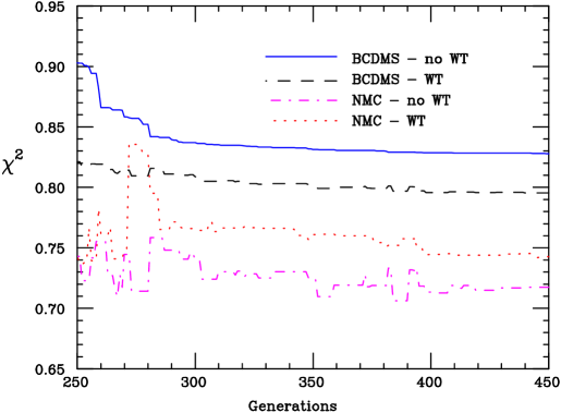
A comparison of a training to experimental data with and without weighted training (WT). As can be seen in the figure, at the end of the neural network training, the $\chi^{2}$ of the two experiments incorporated in the fit (BCDMS and NMC, see Section LABEL:nnqns_appl) are more similar in the case of weighted training than in the case of unweighted training.

An important issue to optimize the efficiency of the neural network training is the choice of the optimal architecture or topology of the neural network. The choice of the architecture of the neural network (the number of layers $L$ and the number of neurons $n_{l}$ in each layer) cannot be derived from general rules and must be tailored to each specific problem. An essential condition is that the neural network has to be redundant, that is, it has to have a larger number of parameters than the minimum number required to satisfactorily fit the patterns we want to learn, in this case experimental data. However, the architecture cannot be arbitrarily large because then the training length becomes very large. A suitable criterion to choose the optimal architecture is to select the architecture which is next to the first stable architecture, that is, the first architecture that can fit the data and gives the same fit than an architecture with one less neuron. This way one is confident that the neural network is redundant for the problem under consideration.

A more systematic approach to determine the optimal architecture of a neural network which parametrizes a function $F$ is related to how many terms are needed in an expansion of $F$ in terms of the activation function $g$. Starting from a large neural network, we can reduce the architecture up to the optimal size with the weight decay approach, in which weights which are rarely updated are allowed to decay according to

$$\delta_{ij}^{(l)}=-\eta\frac{\partial\chi^{2}}{\partial\omega_{ij}^{(l)}}-\epsilon\omega_{ij}^{(l)}\ ,$$ (5.63)

where $\epsilon$ is the decay parameter, typically a small number. This corresponds to adding an extra complexity term to the error function [decayweight],

$$\chi^{2}\to\chi^{2}+\frac{\epsilon}{2\eta}\sum_{i,j,l}\omega_{ij}^{(l)2}\ ,$$ (5.64)

that is, larger weights lead to larger contributions in the error function. A more advanced complexity terms is

$$\chi^{2}\to\chi^{2}+\lambda\sum_{i,j,l}\frac{\omega_{ij}^{(l)2}/\omega_{0}^{2}}{1+\omega_{ij}^{(l)2}/\omega_{0}^{2}}\ ,$$ (5.65)

which again penalizes those weights whose absolute value is larger. With this technique, the network gets forced to only contain the weights that are really needed to represent the problem under consideration.

For each training, the parameters that define the behavior of the neural networks, its weights and thresholds, are initialized at random. To explore in a more efficient way the space of minima, it has been checked to be specially useful to initialize randomly not only the values of the neural network parameters but also the same range in which these parameters are initialized. That is, the parameter initialization range is determined at random between

$$\left[-\left\langle\omega\right\rangle-\sigma_{\omega},\left\langle\omega\right\rangle+\sigma_{\omega}\right]\ ,$$ (5.66)

and

$$\left[-\left\langle\omega\right\rangle+\sigma_{\omega},\left\langle\omega\right\rangle-\sigma_{\omega}\right]\ ,$$ (5.67)

where $\left\langle\omega\right\rangle$ is the average value of the neural network parameters and $\sigma_{\omega}$ is the associated variance.

It has to be taken into account that a minimization strategy is defined not only by an algorithm to vary parameters so that a given quantity is minimized, but also by a convergence condition that determines when the minimization is stopped. Several stopping criteria, each with its own advantages and drawbacks, have been considered during the course of this thesis.

A first criterion is the dynamical stopping of the training. With this criterion, for each replica, we stop the training either when the condition $E^{(k)}\leq\chi^{2}_{\mathrm{stop}}$ is satisfied or, if the previous condition cannot the fulfilled, when the maximum number of iterations of the minimization algorithm $N_{\max}$ is reached. That is, the length of the neural network training is different for each replica. The value of the $\chi^{2}_{\mathrm{stop}}$ parameter is determined by the value of the total $\chi^{2}$, Eq. 5.76, that defines the parametrization. The dynamical stopping of the training allows to avoid both overlearning and insufficient training, as discussed in detail below.

The method to define the optimal value for $N_{\max}$ is the following: first perform a training with a very large value for $N_{\max}$. For $\overline{N}_{\mathrm{rep}}$ replicas, the condition $E^{(k)}\leq\chi^{2}_{\mathrm{stop}}$ will not be satisfied due to statistical fluctuations in the generation of the data replicas. If $E^{(k)}_{N_{\max}}$ is the final value of the error function at the end of the training of the k-th replica, which has not reached the dynamical stopping criterion, then determine for each replica which was the iteration $\mathrm{it}$ for which the condition

$$E^{(k)}_{N^{(k)}_{\mathrm{it}}}\leq\left(1+r_{\chi^{2}}\right)E^{(k)}_{N_{\max}},\qquad N^{(k)}_{\mathrm{it}}\leq N_{\max}\ ,$$ (5.68)

was verified, were $r_{\chi^{2}}$ is the required tolerance. The new and optimal value for $N_{\max}$ is determined then as the average value of such iterations.

$$N_{\max}=\frac{1}{\overline{N}_{\mathrm{rep}}}\sum_{k=1}^{\overline{N}_{\mathrm{rep}}}N^{(k)}_{\mathrm{it}}\ ,$$ (5.69)

where the sum is over those replicas which have not been dynamically stopped. With dynamical stopping of the training, the final distribution of error functions $E^{(k)}$ is even and there is no problem of overlearning, as will be discussed in brief.

An alternative criterion to stop the neural network minimization is fixing the maximum number of iterations of the minimization algorithm to a value large enough so that once is sure that within a given tolerance the fit has converged. However, this approach does not take into account that the length of the training of each replica depends on each precise replica, so it is not computationally efficient and might lead to overlearning.

The rigorous statistical method to determine the value of $\chi^{2}_{\mathrm{stop}}$ with dynamical stopping of the training is the so called overlearning criterion. Since the number of parameters of the neural network parametrization is large, in principle, without the presence of inconsistent data, the final $\chi^{2}$ could be lowered to arbitrarily low values for a large enough neural network. The overlearning criterion to determine the length of the training states that the training should be stopped when the neural network begins to overlearn, that is, it begins to follow the statistical fluctuations of the experimental data rather than the underlying law. The onset of overlearning can be determined by separating the data set into two disjoint sets, called the training set and the validation set. One then minimizes the error function, Eq. 5.34, computed only with the data points of the training set, and analyzes the dependence of the error function of the validation set as a function of the number of iterations.

Then one computes the total $\chi^{2}$, Eq. 5.76, for both the training, $\chi^{2}_{\mathrm{tr}}$, and validation, $\chi^{2}_{\mathrm{val}}$, subsets. It might turn out that statistical fluctuations are large, and one has to average over a large enough number of partitions to obtain stable results. The onset of overlearning is determined as the point in the neural network training such that the $\chi^{2}_{\mathrm{val}}$ of the validation set saturates or even rises while the $\chi^{2}_{\mathrm{tr}}$ of the training set is still decreasing. This implies that the neural network is learning only statistical fluctuations, and signals the point where the training should be stopped.

A drawback of this approach is that one needs to assume that the training subset reproduces the main features of the full set of data points. While this is the case in global fits of parton distributions, where in each kinematical region there are several overlapping measurements, in other physical situations experimental data is much more scarce and the overlearning criterion cannot be used to determine the length of the training.

In Fig. 5.4 we show the expected behavior for the onset of overlearning. One can see that while the $\chi^{2}$ of the validation set begins to increase, the $\chi^{2}$ of the training set is still decreasing. This point signals the onset of overlearning, that is, the fact that the neural network is learning statistical fluctuations rather than the underlying law in the experimental data. Note also that for some problems, like for example those in which the data points are very dense, overlearning could not be possible.

Figure 5.4:

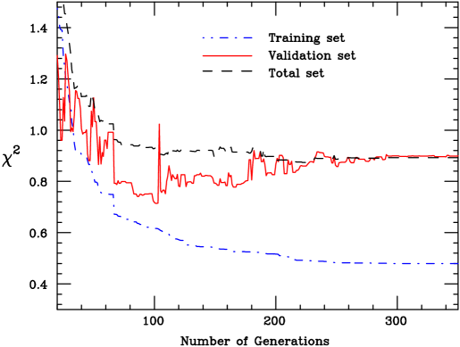
An example of a neural network learning process with overlearning. The point where the $\chi^{2}$ as computed with the validation set begins to rise while the $\chi^{2}$ of the training set is still decreasing is the sign of this overlearning.

An alternative criterion to determine the optimal $\chi^{2}$ which defines the neural network training is the so-called leave-one-out strategy [leaveoneout]. In this strategy, out of the total $N_{\mathrm{dat}}$ data points, one selects one data point at random and leaves it out of the training of all the remaining points. One computes then the prediction of the neural network for this point that has been left out. This procedure is repeated over all the data points, and the total $\chi^{2}$ as computed with the predictions for those points that have been left out is the average $\chi^{2}$ for a pure neural network prediction for a point in the same range. If the underlying law followed by the data points is clear, then the $\chi^{2}$ of a prediction can be as good as the total $\chi^{2}$ of the trained data points, and allows to determine which is the optimal value of the total $\chi^{2}$ to aim for in the neural network training. The conditions for the leave-one-out strategy can be modified to take into account different types of correlations between the data points, for example choosing sets of independent points at random instead of single data points.

5.2.4 Implementation of theoretical constraints

In addition to experimental measurements, in general we have additional theoretical information concerning the function we want to parametrize, like for example kinematical constraints. Since this theoretical information is usually essential to determine the shape of the function that is going to be parametrized, it must be incorporated in our fit. In this section we discuss the different approaches to incorporate theoretical information in our neural network fits. These theoretical constraints are specially useful in general to constrain the shape of the parametrization in regions where there is no experimental data. The methods used in the present thesis have been the following:

1. The Lagrange multipliers method:

   If the function to be parametrized, $F$ has to verify a set of $N_{\mathrm{con}}$ theoretical constraints $\mathcal{F}_{i}\left[F_{i}\right]=\mathcal{F}_{i}^{(\mathrm{theo})}$, one can use the Lagrange multiplier technique, which consist on minimizing for each replica the standard error function while constraining the function to satisfy the theoretical requirements,

   $$\chi^{2(k)}_{\mathrm{tot}}=\chi^{2(k)}_{\mathrm{dat}}+\sum_{i=1}^{N_{\mathrm{con}}}\lambda_{i}\left[\mathcal{F}_{i}\left[F_{i}^{(\mathrm{net})(k)}\right]-\mathcal{F}_{i}^{(\mathrm{theo})}\right]^{2}\ ,$$ (5.70)

   where $\chi^{2(k)}_{\mathrm{dat}}$ is the contribution from the experimental errors, Eqns. 5.33 or 5.34, and where the Lagrange multipliers $\lambda_{i}$ are computed via a stability analysis. They have to be such that the constraints are imposed with the required accuracy but at the same time the space of minima of $\chi^{2(k)}_{\mathrm{tot}}$ has to be close to that of the data error function, $\chi^{2(k)}_{\mathrm{dat}}$.

2. Pseudo-data:

   If the constraints to be imposed of the function $F$ are local, they can be implemented as if they were data points. That is, if the theoretical constraint is

   $$F\left(x_{1},x_{2},\ldots,\tilde{x}_{j},\ldots\right)=b_{j}\ ,$$ (5.71)

   then the minimized quantity should be

   $$\chi^{2(k)}_{\mathrm{tot}}=\chi^{2(k)}_{\mathrm{dat}}+\sum_{j=1}^{N_{\mathrm{con}}}\frac{1}{\sigma_{j}^{2}}\left[F^{(\mathrm{net})(k)}\left(x_{1},x_{2},\ldots,\tilde{x}_{j},\ldots\right)-b_{j}\right]^{2}\ ,$$ (5.72)

   where $\sigma_{j}$ is the accuracy with which the corresponding constraint must be satisfied. This approach differs from the Lagrange multiplier approach in that the accuracy to which the constraints are to be satisfied is fixed by several requirements, for example, by requiring the error $\sigma_{i}$ to be a fixed fraction of the average error of the experimental data points. Note that this is equivalent to adding to the experimental data set artificial data points with central value $F\left(x_{1},x_{2},\ldots,\tilde{x}_{j},\ldots\right)=b_{j}$ and total uncorrelated error $\sigma_{j}$. The addition of artificial data points is helpful to constrain the shape of the parametrized function in regions without experimental data, for example near kinematical thresholds.

3. Hard-wired parametrization:

   Another method is to hard-wire the constraint in the neural network parametrization. This method is specially useful to implement the vanishing of the function for some kinematical region. If we have

   $$F\left(x_{1},x_{2},\ldots,\tilde{x}_{j},\ldots\right)=0\ ,$$ (5.73)

   then we redefine the function to be parametrized to be

   $$F^{(\mathrm{net})(k)}\left(x_{1},x_{2},\ldots\right)\equiv\prod_{j=1}^{N_{\mathrm{con}}}\left(x_{j}-\tilde{x}_{j}\right)^{n_{j}}\overline{F}^{(\mathrm{net})(k)}\left(x_{1},x_{2},\ldots\right)\ ,$$ (5.74)

   where now is the function $\overline{F}^{(\mathrm{net})}$ the one that is going to be parametrized with a neural network. The introduction of a partial functional form dependence in the parametrization does not mean that there is any functional form bias, since one can check the the results of the fit do not depend on the values of $n_{j}$, provided they verify $n_{j}>0$. The default values of the $n_{j}$ parameters have to be determined from a stability analysis to assess which is the optimal neural network training preprocessing.

All of the above techniques can be combined for a given parametrization. Using any of these techniques, it has to be shown that in each case the result of the fit is modified as expected by the implementation of the kinematical constraints. For example, the dominant contribution to $\chi^{2}_{\mathrm{tot}}$ has to be always that of the experimental data points.

5.3 Validation of the results

The third step of our strategy consists on the validation of the results of the neural network training using suitable statistical estimators. These results are defined by the sample of trained neural networks which constitutes the sought-for probability measure for the observable $F$, $\mathcal{P}\left[F\right]$, from which expectation values for an arbitrary functional of it, $\mathcal{F}[F]$, can be computed using

$$\left\langle\mathcal{F}[F]\right\rangle=\int\mathcal{D}F\mathcal{P}\left[F\right]\mathcal{F}[F]=\frac{1}{N_{\mathrm{rep}}}\sum_{k=1}^{N_{\mathrm{rep}}}\mathcal{F}[F^{(\mathrm{net})(k)}]\ ,$$ (5.75)

just as with standard probability measures. We define now such estimators, that can be divided into two categories: statistical estimators to assess how well the sample of trained neural networks reproduce the features of the experimental data, and statistical estimators which assess the stability of a given fit with respect some parameters, for example the number of trained neural networks.

5.3.1 Statistical estimators: probability measure vs. experimental data

Now we describe the statistical estimators that we use to assess the quality of the constructed probability measure in the space of the observable $F$ by comparing with the experimental data. The goodness of the final fit is measured with the total $\chi^{2}$, as constructed from the full experimental covariance matrix

$$\chi^{2}=\frac{1}{N_{\mathrm{dat}}}\sum_{i,j=1}^{N_{\mathrm{dat}}}\left(\left\langle F_{i}^{(\mathrm{net})}\right\rangle_{\mathrm{rep}}-F_{i}^{(\mathrm{exp})}\right)\left(\mathrm{cov}^{-1}\right)_{ij}\left(\left\langle F_{j}^{(\mathrm{net})}\right\rangle_{\mathrm{rep}}-F_{j}^{(\mathrm{exp})}\right)\ ,$$ (5.76)

where now the total experimental covariance matrix Eq. 5.6 includes the contribution from the normalization uncertainties. If experimental errors were correctly estimated and there were no incompatibilities between measurements, on statistical grounds one would expect $\chi^{2}\sim 1$, with deviations from this value scaling with the number of data points as $1/\sqrt{N_{\mathrm{dat}}}$. To be precise, instead of $N_{\mathrm{dat}}$ one should have the number of degrees of freedom $N_{\mathrm{dof}}$, the difference between the number of data points and the number of free parameters of the theoretical model $N_{\mathrm{par}}$, and the standard deviation of the $\chi^{2}$ distribution is given by $\sigma_{\chi^{2}}=\sqrt{2/N_{\mathrm{dof}}}$.

Another important estimator is the average error,

$$\left\langle E\right\rangle=\frac{1}{N_{\mathrm{rep}}}\sum_{k=1}^{N_{\mathrm{rep}}}E^{(k)}\ ,$$ (5.77)

where $E^{(k)}$ is either Eq. 5.33 or Eq. 5.34, depending on the estimator which has been used in the neural network training. It is instructive to estimate the typical values that the average error Eq. 5.77 can take. We will compute now Eq. 5.77 in a simplified model, in which correlated systematics are neglected. Let us consider a set of measurement $m_{i}$ of $F$. Then if one assumes that experimental measurements are distributed gaussianly around the true value $t_{i}$ of the observable, one has

$$m_{i}=t_{i}+\sigma_{i}s_{i}\ ,$$ (5.78)

where $\sigma_{i}$ is the total error and $s_{i}$ a univariate zero mean gaussian number. The k-th replica of generated artificial data $g^{(k)}$ is as in Eq. 5.3 without correlated uncertainties,

$$g_{i}^{(k)}=m_{i}+r_{i}^{(k)}\sigma_{i}=t_{i}+(s_{i}+r_{i}^{(k)})\sigma_{i}\ ,$$ (5.79)

where $r_{i}^{k}$ is another univariate zero mean gaussian random number. Now let us assume that the best fit neural networks are distributed around the true values of the observable $F$ with error $\hat{\sigma}_{i}$. For the k-th neural network $n^{(k)}$ we will have

$$n_{i}^{(k)}=t_{i}+l_{i}^{(k)}\hat{\sigma}_{i}\ ,$$ (5.80)

where $l_{i}^{(k)}$ are highly correlated to both $r_{i}^{(k)}$ and $t_{i}$. For a large enough set of measurements, and a large enough number of generated replicas, so that correlations between $s_{i}$ and $r_{i}^{(k)}$ can be neglected, it can be seen that the average error is given by,

$$\left\langle E\right\rangle_{\mathrm{rep}}=2+\left\langle\frac{\hat{\sigma}^{2}}{\sigma^{2}}\right\rangle_{\mathrm{dat}}-2\left\langle\left\langle rl\right\rangle_{\mathrm{rep}}\frac{\hat{\sigma}}{\sigma}\right\rangle_{\mathrm{dat}}\ ,$$ (5.81)

where the error function is the diagonal error, Eq. 5.33. Note also that within the same model, the error function of the k-th net as compared to the experimental measurement, defined as

$$\widetilde{E}^{(k)}_{2}=\frac{1}{N_{\mathrm{dat}}}\sum_{i=1}^{N_{\mathrm{dat}}}\frac{\left(m_{i}-n_{i}^{(k)}\right)^{2}}{\sigma^{2}_{\mathrm{stat},i}}\ ,$$ (5.82)

has as average

$$\left\langle\widetilde{E}\right\rangle_{\mathrm{rep}}=1+\left\langle\frac{\hat{\sigma}^{2}}{\sigma^{2}}\right\rangle_{\mathrm{dat}}\geq 1\ ,$$ (5.83)

and finally in the case that the neural network prediction coincides with the true value of the function, $\hat{\sigma}_{i}=0$, the average error is $\left\langle\tilde{E}\right\rangle_{\mathrm{rep}}=1$, just as expected from textbook statistics.

Now we define the estimators which are used to assess how well the sample of trained neural networks reproduce the sample of experimental data. These estimators are

• Average for each experimental point

  $$\left\langle F_{i}^{(\mathrm{net})}\right\rangle_{\mathrm{rep}}=\frac{1}{N_{\mathrm{rep}}}\sum_{k=1}^{N_{\mathrm{rep}}}F_{i}^{(\mathrm{net})(k)}\ .$$ (5.84)

• Associated variance

  $$\sigma_{i}^{(\mathrm{net})}=\sqrt{\left\langle\left(F_{i}^{(\mathrm{net})}\right)^{2}\right\rangle_{\mathrm{rep}}-\left\langle F_{i}^{(\mathrm{net})}\right\rangle^{2}_{\mathrm{rep}}}\ .$$ (5.85)

• Associated covariance

  $$\rho_{ij}^{(\mathrm{net})}=\frac{\left\langle F_{i}^{(\mathrm{net})}F_{j}^{(\mathrm{net})}\right\rangle_{\mathrm{rep}}-\left\langle F_{i}^{(\mathrm{net})}\right\rangle_{\mathrm{rep}}\left\langle F_{j}^{(\mathrm{net})}\right\rangle_{\mathrm{rep}}}{\sigma_{i}^{(\mathrm{net})}\sigma_{j}^{(\mathrm{net})}}\ .$$ (5.86)

  $$\mathrm{cov}_{ij}^{(\mathrm{net})}=\rho_{ij}^{(\mathrm{net})}\sigma_{i}^{(\mathrm{net})}\sigma_{j}^{(\mathrm{net})}\ .$$ (5.87)

  As in the case of the artificial replicas, the three above quantities provide the estimators of the experimental central values, errors and correlations as computed from the sample of trained neural networks.

• Mean variance and percentage error on central values over the $N_{\mathrm{dat}}$ data points.

  $$\left\langle V\left[\left\langle F^{(\mathrm{net})}\right\rangle_{\mathrm{rep}}\right]\right\rangle_{\mathrm{dat}}=\frac{1}{N_{\mathrm{dat}}}\sum_{i=1}^{N_{\mathrm{dat}}}\left(\left\langle F_{i}^{(\mathrm{net})}\right\rangle_{\mathrm{rep}}-F_{i}^{(\mathrm{exp})}\right)^{2}\ ,$$ (5.88)

  $$\left\langle PE\left[\left\langle F^{(\mathrm{net})}\right\rangle_{\mathrm{rep}}\right]\right\rangle_{\mathrm{dat}}=\frac{1}{N_{\mathrm{dat}}}\sum_{i=1}^{N_{\mathrm{dat}}}\left[\frac{\left\langle F_{i}^{(\mathrm{net})}\right\rangle_{\mathrm{rep}}-F_{i}^{(\mathrm{exp})}}{F_{i}^{(\mathrm{exp})}}\right]\ .$$ (5.89)

  We define analogously the mean variance and the percentage error for errors, correlations and covariances.

• Scatter correlation

  $$r\left[F^{(\mathrm{net})}\right]=\frac{\left\langle F^{(\mathrm{exp})}\left\langle F^{(\mathrm{net})}\right\rangle_{\mathrm{rep}}\right\rangle_{\mathrm{dat}}-\left\langle F^{(\mathrm{exp})}\right\rangle_{\mathrm{dat}}\left\langle\left\langle F^{(\mathrm{net})}\right\rangle_{\mathrm{rep}}\right\rangle_{\mathrm{dat}}}{\sigma_{s}^{(\mathrm{exp})}\sigma_{s}^{(\mathrm{net})}}\ ,$$ (5.90)

  where the scatter variance $\sigma_{s}^{(\mathrm{net})}$ associated to the neural network prediction is defined as

  $$\sigma_{s}^{(\mathrm{net})}=\sqrt{\left\langle\left(\left\langle F^{(\mathrm{net})}\right\rangle_{\mathrm{rep}}\right)^{2}\right\rangle_{\mathrm{dat}}-\left(\left\langle\left\langle F^{(\mathrm{net})}\right\rangle_{\mathrm{rep}}\right\rangle_{\mathrm{dat}}\right)^{2}}\ .$$ (5.91)

  We define analogously $r[\sigma^{(\mathrm{net})}]$, $r[\rho^{(\mathrm{net})}]$ and $r[\mathrm{cov}^{(\mathrm{net})}]$.

• ${\cal R}$-ratio

  $${\cal R}=\frac{\langle\tilde{E}\rangle}{\langle E\rangle},$$ (5.92)

  where ${\langle E\rangle}$ is given by Eq. 5.77, with covariance matrix error, and for $\tilde{E}^{(k)}$ one uses the analog of Eq. 5.82 including correlated errors,

  $$\left\langle\widetilde{E}\right\rangle=\frac{1}{N_{\mathrm{rep}}}\sum_{k=1}^{N_{\mathrm{rep}}}{\widetilde{E}}^{(k)}\ ,$$ (5.93)

  $${\widetilde{E}}^{(k)}=\frac{1}{N_{\mathrm{dat}}}\sum_{i,j=1}^{N_{\mathrm{dat}}}\left(F_{i}^{(\mathrm{net})(k)}-F_{i}^{(\exp)}\right){\overline{\mathrm{cov}}^{(k)}}^{-1}_{ij}\left(F_{j}^{(\mathrm{net})(k)}-F_{j}^{(\exp)}\right)\ .$$ (5.94)

  The $\mathcal{R}-$ratio is interesting since it provides an estimator which is capable to determine whether or not when error reduction is observed it is due to the fact that the neural network by combining data points has found the underlying law or whether in the other hand it is due to artificial smoothing. To verify this property, assume that correlated systematic uncertainties can be neglected, as we have done in the example above, then the estimator reads

  $$\mathcal{R}=\frac{1+\left\langle\frac{\hat{\sigma}^{2}}{\sigma^{2}}\right\rangle_{\mathrm{dat}}}{2+\left\langle\frac{\hat{\sigma}^{2}}{\sigma^{2}}\right\rangle_{\mathrm{dat}}-2\left\langle\left\langle rl\right\rangle_{\mathrm{rep}}\frac{\hat{\sigma}}{\sigma}\right\rangle_{\mathrm{dat}}}\ ,$$ (5.95)

  so that if error reduction is due to the fact that the neural network has found the underlying law that describes the experimental data, one will have $\hat{\sigma}\ll\sigma$ and therefore the $\mathcal{R}$-ratio will satisfy $\mathcal{R}\sim 1/2$.

Note that even if the covariance matrix is determined from the correlation matrix and the total error from Eq. 5.7, the reproduction of covariances by the probability measure has to be validated independently of correlations and error. This is so because even if it is clear that when correlations and errors are correctly reproduced, also covariances will be reproduced, the inverse is not necessarily true.

5.3.2 Statistical estimators: stability of the probability measure

Let us define the statistical estimators that are used to analyze the compatibility and stability of the constructed probability measure with respect of some of the parameters that define the fit. These estimators are also useful in order to perform a quantitative comparison between fits, that is, between probability measures. For example, we know how the different estimators depend on the size of the sample $N_{\mathrm{rep}}$ in the replica generation, but we do not know if the same behavior holds for the sample of trained networks. The estimators in the above section were used to compare the results of either the replica generation or the neural network fit to  experimental data. In this section we want to define statistical estimators which allow us to compare a given fit with another fit. Since in practical applications we will have a reference fit, and compare other fits with it, let us label the first fit as the reference fit and is denoted by the superscript (ref) and the second fit as the current fit, denoted by the superscript (fit).

These estimators are divided in estimators for central values, standard deviations and correlations. The estimators are computed for a set of $\widetilde{N}_{\mathrm{dat}}$ points which need not to be the same points where there is experimental data. In particular one can compute these estimators in the extrapolation region, to check the stability of the fit also in the region where there is no experimental data. These estimators are given by:

• Central values:

  • Relative error:

    $$\left\langle\mathrm{RE}\left[F\right]\right\rangle_{\mathrm{dat}}=\frac{1}{\widetilde{N}_{\mathrm{dat}}}\sum_{i=1}^{\widetilde{N}_{\mathrm{dat}}}\Bigg{|}2\left(\frac{\left\langle F_{i}^{(\mathrm{ref})}\right\rangle-\left\langle F_{i}^{(\mathrm{fit})}\right\rangle}{\sqrt{V\left[F_{i}^{(\mathrm{ref})}\right]}+\sqrt{V\left[F_{i}^{(\mathrm{fit})}\right]}}\right)\Bigg{|}\equiv\left\langle\Bigg{|}2\frac{\left\langle F_{i}^{(\mathrm{ref})}\right\rangle-\left\langle F_{i}^{(\mathrm{fit})}\right\rangle}{\sqrt{V\left[F_{i}^{(\mathrm{ref})}\right]}+\sqrt{V\left[F_{i}^{(\mathrm{fit})}\right]}}\Bigg{|}\right\rangle_{\mathrm{dat}}\ ,$$ (5.96)

  • Scatter correlation:

    $$r\left[\left\langle F\right\rangle\right]=\frac{\left\langle\left\langle F^{(\mathrm{fit})}F^{(\mathrm{ref})}\right\rangle\right\rangle_{\mathrm{dat}}-\left\langle\left\langle F^{(\mathrm{fit})}\right\rangle\right\rangle_{\mathrm{dat}}\left\langle\left\langle F^{(\mathrm{ref})}\right\rangle\right\rangle_{\mathrm{dat}}}{\sqrt{\left\langle\left\langle F^{(\mathrm{fit})2}\right\rangle\right\rangle_{\mathrm{dat}}-\left\langle\left\langle F^{(\mathrm{fit})}\right\rangle\right\rangle_{\mathrm{dat}}^{2}}\sqrt{\left\langle\left\langle F^{(\mathrm{ref})2}\right\rangle\right\rangle_{\mathrm{dat}}-\left\langle\left\langle F^{(\mathrm{ref})}\right\rangle\right\rangle_{\mathrm{dat}}^{2}}}\ .$$ (5.97)

• Standard deviations:
  

  • Relative error:

    $$\left\langle\mathrm{RE}\left[\sigma^{2}\right]\right\rangle=\frac{1}{\widetilde{N}_{\mathrm{dat}}}\sum_{i=1}^{\widetilde{N}_{\mathrm{dat}}}\Bigg{|}2\frac{\sigma_{i}^{(\mathrm{ref})2}-\sigma_{i}^{(\mathrm{fit})2}}{\sqrt{V\left[\sigma_{i}^{(\mathrm{fit})}\right]}+\sqrt{V\left[\sigma_{i}^{(\mathrm{ref})}\right]}}\Bigg{|}=\left\langle 2\Bigg{|}\frac{\sigma_{i}^{(\mathrm{ref})2}-\sigma_{i}^{(\mathrm{fit})2}}{\sqrt{V\left[\sigma_{i}^{(\mathrm{fit})}\right]}+\sqrt{V\left[\sigma_{i}^{(\mathrm{ref})}\right]}}\Bigg{|}\right\rangle_{\mathrm{dat}}\ ,$$ (5.98)

  • Scatter correlation:

    $$r\left[\sigma\right]=\frac{\left\langle\left\langle\sigma^{(\mathrm{fit})}\sigma^{(\mathrm{ref})}\right\rangle\right\rangle_{\mathrm{dat}}-\left\langle\sigma^{(\mathrm{fit})}\right\rangle_{\mathrm{dat}}\left\langle\sigma^{(\mathrm{ref})}\right\rangle_{\mathrm{dat}}}{\sqrt{\left\langle\sigma^{(\mathrm{fit})2}\right\rangle_{\mathrm{dat}}-\left\langle\sigma^{(\mathrm{fit})}\right\rangle_{\mathrm{dat}}^{2}}\sqrt{\left\langle\sigma^{(\mathrm{ref})2}\right\rangle_{\mathrm{dat}}-\left\langle\sigma^{(\mathrm{ref})}\right\rangle_{\mathrm{dat}}^{2}}}\ .$$ (5.99)

• Correlations:
  

  • Relative error:

    $$\left\langle\mathrm{RE}\left[\rho\right]\right\rangle=\frac{1}{\widetilde{N}_{\mathrm{dat}}\left(\widetilde{N}_{\mathrm{dat}}+1\right)/2}\sum_{i=1}^{\widetilde{N}_{\mathrm{dat}}}\sum_{j=i}^{\widetilde{N}_{\mathrm{dat}}}\Bigg{|}2\frac{\rho_{ij}^{(\mathrm{ref})}-\rho_{ij}^{(\mathrm{fit})}}{\sqrt{V\left[\rho_{ij}^{(\mathrm{fit})}\right]}+\sqrt{V\left[\rho_{ij}^{(\mathrm{ref})}\right]}}\Bigg{|}\equiv$$

    $$\left\langle\Bigg{|}2\frac{\rho_{ij}^{(\mathrm{ref})}-\rho_{ij}^{(\mathrm{fit})}}{\sqrt{V\left[\rho_{ij}^{(\mathrm{fit})}\right]}+\sqrt{V\left[\rho_{ij}^{(\mathrm{ref})}\right]}}\Bigg{|}\right\rangle_{\mathrm{dat}}\qquad\qquad\qquad\ ,$$ (5.100)

  • Scatter correlation:

    $$r\left[\rho\right]=\frac{\left\langle\left\langle\rho^{(\mathrm{fit})}\rho^{(\mathrm{ref})}\right\rangle\right\rangle_{\mathrm{dat}}-\left\langle\rho^{(\mathrm{fit})}\right\rangle_{\mathrm{dat}}\left\langle\rho^{(\mathrm{ref})}\right\rangle_{\mathrm{dat}}}{\sqrt{\left\langle\rho^{(\mathrm{fit})2}\right\rangle_{\mathrm{dat}}-\left\langle\rho^{(\mathrm{fit})}\right\rangle_{\mathrm{dat}}^{2}}\sqrt{\left\langle\rho^{(\mathrm{ref})2}\right\rangle_{\mathrm{dat}}-\left\langle\rho^{(\mathrm{ref})}\right\rangle_{\mathrm{dat}}^{2}}}\ .$$ (5.101)

were averages and variances of central values, errors and correlations can be computed using the expressions in Appendix LABEL:probrev. Two probability measures are said to be equivalent to each other if the conditions $\left\langle\mathrm{RE}\left[F\right]\right\rangle_{\mathrm{dat}}\mathrel{\hbox to0.0pt{\lower 4.0pt\hbox{\hskip 1.0pt$\sim$}\hss}\raise 1.0pt\hbox{$<$}}1$, $\left\langle\mathrm{RE}\left[\sigma^{2}\right]\right\rangle_{\mathrm{dat}}\mathrel{\hbox to0.0pt{\lower 4.0pt\hbox{\hskip 1.0pt$\sim$}\hss}\raise 1.0pt\hbox{$<$}}1$ and $\left\langle\mathrm{RE}\left[\rho\right]\right\rangle_{\mathrm{dat}}\mathrel{\hbox to0.0pt{\lower 4.0pt\hbox{\hskip 1.0pt$\sim$}\hss}\raise 1.0pt\hbox{$<$}}1$ are fulfilled. For the scatter correlations one expects for two compatible probability measures the condition $r\mathrel{\hbox to0.0pt{\lower 4.0pt\hbox{\hskip 1.0pt$\sim$}\hss}\raise 1.0pt\hbox{$<$}}1$ to hold. Note that the $\widetilde{N}_{\mathrm{dat}}$ points where the stability estimators defined above are computed do not need to be those were there is experimental data, for instance, these estimators can be used to compute the stability of a probability measure also in the extrapolation region. Since fluctuations might be large, it might be needed to average over different partitions of the sets of trained neural networks to obtain stable results.

Another relevant estimator is the so called pull. The average pull of two different fits is defined as

$$\left\langle P\right\rangle_{\mathrm{dat}}=\frac{1}{N_{\mathrm{dat}}}=\sum_{i=1}^{N_{\mathrm{dat}}}P_{i}=\sum_{i=1}^{N_{\mathrm{dat}}}\frac{\left\langle F_{i}^{(\mathrm{ref})}\right\rangle-\left\langle F_{i}^{(\mathrm{fit})}\right\rangle}{\sqrt{\sigma_{i}^{(\mathrm{fit})2}+\sigma_{i}^{(\mathrm{ref})2}}}\ ,$$ (5.102)

For two fits to be consistent within the respective uncertainties the condition $P_{i}\mathrel{\hbox to0.0pt{\lower 4.0pt\hbox{\hskip 1.0pt$\sim$}\hss}\raise 1.0pt\hbox{$<$}}1$ should be satisfied. Note that the condition $P_{i}\leq 1$ is necessary for two fits to be compatible within errors, but it is not sufficient for two fits to define the same probability measure, since in particular, if either $\sigma^{(\mathrm{fit})}$ or $\sigma^{(\mathrm{ref})}$ is much larger than the other error, then the two fits will be very different yet the pull will still satisfy $P_{i}\leq 1$.

Finally, there are other conditions that must be verified for the sample of trained neural networks for a given fit to be considered as satisfactory. These conditions are related to the criteria used to stop the minimization of the individual replicas. If we use dynamical stopping of the training, as described in Section 5.2.2, the distribution of errors $E^{(k)}$ at the end of the training over the trained replica sample must be peaked around the average result $\left\langle E\right\rangle$, Eq. 5.77, because the opposite case would mean that the averaged result is obtained combining good fits with bad fits (in the sense of fits with large values of $E^{(k)}$). Another estimator of the consistency of the results is the distribution of training length, where the training length measures the length of the minimization procedure, cannot be peaked near $N_{\max}$, the maximum number of iterations, because if it is this means that the dynamical stopping of the minimization is not being effective, and one has instead fixed training length minimization. In Section 6.3 we show how these two conditions are satisfied in a particular example.

Chapter 6 The neural network approach: Applications

In this Chapter we review four applications of the general strategy to parametrize experimental data that has been described in the previous Chapter. First we describe a parametrization of the vector-axial vector spectral function $\rho_{V-A}(s)$ from the hadronic decays of the tau lepton which incorporates theoretical information in the form of sum rules, with the motivation of extracting from this parametrization the values of the nonperturbative vacuum condensates. Then we present a parametrization of the proton structure function $F_{2}^{p}(x,Q^{2})$, which updates the results of Ref. [f2ns] by including the data from the HERA experiments. This parametrization is not only interesting as a new application of the general technique, but also it allows us to develop the necessary techniques to apply our general strategy to problems with data coming from many different experiments. The third application is a parametrization of the lepton energy distribution $d\Gamma(E_{l})/dE_{l}$ in the semileptonic decays of the B meson. As a byproduct of this parametrization we will provide a determination of the b quark mass $\overline{m}_{b}\left(\overline{m}_{b}\right)$.

We devote special attention to the last and most important application, which is the main motivation for the development of the techniques described in Chapter 5: the neural network parametrization of parton distributions. To this purpose a new strategy to solve the DGLAP evolution equations is introduced. We then review the parametrization of the non-singlet parton distribution $q_{NS}(x,Q_{0}^{2})$ from experimental data on the non-singlet structure function $F_{2}^{NS}(x,Q^{2})$, and we devote special attention to the comparison of our results with those of the standard approach to parton distributions described in Section 4.2.

6.1 Spectral functions in hadronic tau decays

In this Section, we describe the first application of the technique introduced in Chapter 5 to parametrize experimental data that was implemented during the present thesis. We construct a parametrization of the vector minus axial-vector spectral function $\rho_{V-A}(s)$ from the hadronic decays of the tau lepton. As has been described in Section 4.1.4, this spectral function is determined from purely nonperturbative dynamics, so it is specially suited for the determination of non perturbative parameters like the chiral vacuum condensates. The motivation to determine a parametrization of the spectral function $\rho_{V-A}(s)$ is thus to provide an extraction of the QCD vacuum condensates $\left\langle\mathcal{O}_{6}\right\rangle$, $\left\langle\mathcal{O}_{8}\right\rangle$ and higher dimensional condensates from experimental data. A more detailed description of this work can be found in Ref. [condensates].

Following the strategy described in the previous Chapter, the parametrization of the spectral function $\rho_{V-A}(s)$ will combine all available experimental information, that is, central values, errors and correlations, together with information from theoretical constraints: the chiral sum rules, Eqns. 4.62-4.65 and the asymptotic vanishing of the spectral function in the perturbative $s\to\infty$ limit, Eq. 4.56. This way we will obtain a determination of the QCD vacuum condensates which is unbiased with respect to the parametrization of the spectral function and with faithful estimation and propagation of the experimental uncertainties. All sources of uncertainty related to the method of analysis are kept under control, and their contribution to the total error in the extraction of the condensates is estimated, as discussed in [condensates].

Since the relevant spectral function for the determination of the condensates is the $\rho_{V-A}(s)$ spectral function, we need a simultaneous measurement of the vector and axial-vector spectral functions from the hadronic decays of the tau lepton. Data from the ALEPH Collaboration [exp1] and from the OPAL Collaboration [expopal] will be used, which provide a simultaneous determination of the vector and axial vector spectral functions in the same kinematic region and also provide the full set of correlated uncertainties for these measurements. There exists additional data on spectral functions coming from electron-positron annihilation, but their quality is lower than the data from hadronic tau decays and will not be incorporated to the present analysis.

Experimental data does not consist on the spectral function directly, but rather on the invariant mass-squared spectra for both the vector and axial-vector components, that are related to the spectral functions by a kinematic factor and a branching ratio normalization,

$$\rho_{V/A}(s)\equiv\frac{M^{2}_{\tau}}{6|V_{ud}|^{2}S_{EW}}\frac{B(\tau^{-}\to V^{-}/A^{-}\nu_{\tau})}{B(\tau^{-}\to e^{-}\bar{\nu}_{e}\nu_{\tau})}\frac{1}{N_{V/A}}\frac{dN_{V/A(s)}}{ds}\left[\left(1-\frac{s}{M_{\tau}^{2}}\right)\left(1-\frac{2s}{M_{\tau}^{2}}\right)\right]^{-1}\ ,\quad s\leq M_{\tau}^{2}\ .$$ (6.1)

In the above equation,

$$\frac{1}{N_{V/A}}\frac{dN_{V/A}(s)}{ds}\ ,$$ (6.2)

is the normalized invariant mass distribution, $M_{\tau}$ is the tau lepton mass, $s$ is the invariant mass of the hadronic final state and $S_{EW}$ are the electroweak radiative corrections.

In the following $\rho^{(\exp)}_{V-A,i}$ will denote the $i$-th data point,

$$\rho^{(\exp)}_{V-A,i}=\rho_{V-A}(s_{i})\equiv\rho_{V}(s_{i})-\rho_{A}(s_{i})\ ,\qquad i=1,\ldots,N_{\mathrm{dat}}\ ,$$ (6.3)

where $N_{\mathrm{dat}}$ is the number of available data points. Fig. 6.1 shows the experimental data used in the present analysis from the two LEP experiments. Note that errors are small in the low and middle $s$ regions and that they become larger as we approach the tau mass threshold. The last points are almost zero in the invariant mass spectrum, since near threshold the reduced phase space implies a lack of statistics, and are only enhanced in the spectral functions due to the large kinematic factor for $s$ near $M_{\tau}^{2}$ (the last term in Eq. 6.1), so special care must be taken with the physical significance of these points.

Figure 6.1:

Experimental data for $\rho_{V-A}(s)$ spectral function from the ALEPH (left) and OPAL (right) collaborations. Note that errors increase as we approach the kinematic threshold at $s=M_{\tau}^{2}$.

It is clear that the asymptotic vanishing of the spectral function,

$$\lim_{s\to\infty}\rho_{V-A}(s)\to 0\ ,$$ (6.4)

implied by perturbative QCD is not reached for $s\leq M_{\tau}^{2}$, at least for the central experimental values, and therefore should be enforced artificially on the parametrization of the $\rho_{V-A}(s)$ spectral function that we will construct. The method that we use takes advantage of the smooth, unbiased interpolation capability of neural networks: artificial points are added to the data set with adjusted errors in a region where $s$ is high enough that the $\rho_{V-A}(s)$ spectral function should vanish, as discussed in Section 5.2.4. That is, we add to the experimental data a set of artificial points,

$$\rho_{V-A}(s_{i})=\ 0,\qquad i=N_{\mathrm{dat}}+1,\ldots,N_{\mathrm{tot}}\ ,\qquad s_{i}\geq M_{\tau}^{2}\ ,$$ (6.5)

with error $\sigma_{i}$, and where $N_{\mathrm{tot}}$ is the total number of points (data and artificial). Once these artificial points are included, the neural network will smoothly interpolate between the real and artificial data points, also taking into account the constraints of the sum rules, as explained below.

$\rho_{V-A}(s)$
$N_{\mathrm{rep}}$	10	100	1000
$r[\rho_{V-A}(s)^{(\mathrm{art})}]$	0.98	0.99	0.99
$r[\sigma^{(\mathrm{art})}]$	0.98	0.99	0.99
$r[\rho^{(\mathrm{art})}]$	0.61	0.95	0.99

Table 6.1:

Comparison between experimental data the Monte Carlo sample of artifical replicas for the $\rho_{V-A}(s)$ spectral function.

As has been described in Chapter 5, the first step in the parametrization of the spectral function $\rho_{V-A}(s)$ is the generation of a Monte Carlo sample of replicas of the experimental data. The experimental data for the invariant hadronic mass spectrum consist on the central values, the total error and the correlations between different invariant mass bins. Therefore, to generate replicas of the experimental data, we use Eq. 5.13, which in the present case reads

$$\rho_{V-A,i}^{(\mathrm{art})(k)}=\rho_{V-A,i}^{(\exp)}+r_{i}^{(k)}\sigma_{\mathrm{tot},i}\ ,\qquad k=1,\ldots,N_{\mathrm{rep}}\ ,$$ (6.6)

where the gaussian random numbers $r_{i}^{(k)}$ have the same correlation as experimental data. The replica generation has the statistical estimators that can be seen in Table 6.1. It can be seen that a Monte Carlo sample with $N_{\mathrm{rep}}=1000$ is required to have scatter correlations larger than 0.99 for both central values, errors and correlations.

Once the Monte Carlo sample of replicas has been generated, following the method described above, one has to train a neural network in each replica. The estimator which will be minimized in the present case is the diagonal error Eq. 5.33, which reads

$$E_{2}^{(k)}=\frac{1}{N_{\mathrm{tot}}}\sum_{k=1}^{N_{\mathrm{tot}}}\frac{\left(\rho_{V-A,i}^{(\mathrm{art})(k)}-\rho_{V-A,i}^{(\mathrm{net})(k)}\right)^{2}}{\sigma_{\mathrm{stat},i}^{2}}\ ,\quad k=1,\ldots,N_{\mathrm{rep}}\ ,$$ (6.7)

where $\rho_{V-A,i}^{(\mathrm{net})(k)}$ is the k-th neural network, trained on the k-th replica of the experimental data. Note that as explained in [f2ns], correlations are correctly incorporated in the parametrization of $\rho_{V-A}(s)$ through the Monte Carlo pseudo-data generation, Eq. 6.6. As has been described in Section 4.1.4, the parametrization of the $\rho_{V-A}(s)$ spectral function has to satisfy several theoretical constraints. These theoretical constraints, the chiral sum rules, are implemented using the Lagrange Multipliers technique, as described in Section 5.2.4. Therefore the total error function to be minimized will be

$$E_{\mathrm{tot}}^{(k)}=E_{2}^{(k)}+\sum_{i=1}^{N_{\mathrm{con}}}\lambda_{i}\left(\mathcal{F}_{i}\left(\rho_{V-A}^{(\mathrm{net})(k)}(s)\right)-\mathcal{F}_{i}^{(\mathrm{theo})}\right)^{2}\ ,$$ (6.8)

where for example, for the first theoretical constraint, the DMO sum rule, Eq. 4.62, one has

$$\mathcal{F}_{1}\left[\rho_{V-A}^{(\mathrm{net})(k)}(s)\right]=\frac{1}{4\pi^{2}}\int_{0}^{\infty}ds\frac{\rho_{V-A}^{(\mathrm{net})(k)}(s)}{s},\qquad\mathcal{F}_{i}^{(\mathrm{theo})}=\frac{f_{\pi}\left\langle r_{\pi}^{2}\right\rangle}{3}-F_{A}\ ,$$ (6.9)

and similarly for the remaining chiral sum rules, up to $N_{\mathrm{con}}=4$. These sum rules act as constraints on the neural network output, that is, the main contribution to the error function $E_{\mathrm{tot}}^{(k)}$ (which determines the learning of the network) still comes from the experimental errors, that is, the $E_{2}^{(k)}$ term, and the sum rules are only relevant in the region where the errors are larger. The relative weights of the chiral sum rules $\lambda_{i}$ are determined according to a stability analysis, as discussed in [condensates].

The length of the training is fixed by studying the behavior of the error function $E_{\mathrm{tot}}^{(0)}$ for the neural net fitted to the central experimental values, and asking that $E_{\mathrm{tot}}^{(0)}$ stabilizes to a value close to one, which on statistical grounds in the value expected for a correct fit. The minimization algorithm that is used for the neural network training is Genetic Algorithms, introduced in Section 5.2.3, which is required since the total error function to be minimized, Eq. 6.8, depends non-linearly with the $\rho_{V-A}(s)$ spectral function through the convolutions of the chiral sum rules.

With the strategy discussed above, $N_{\mathrm{rep}}$ neural networks are trained on the $N_{\mathrm{rep}}$ Monte Carlo replicas of the experimental data for the spectral function $\rho_{V-A}(s)$. As has been described in Chapter 5, once the probability measure in the space of spectral functions $\mathcal{P}\left[\rho_{V-A}\right]$ has been constructed, it is crucial to validate the results with suitable statistical estimators. A number of checks is then performed in order to be sure that an unbiased representation of the probability density has been obtained. The values for the scatter correlations for central values, errors and correlations are presented in Table 6.2. It is seen that the central values and the correlations are well reproduced, whereas this is not the case for the total errors. The average standard deviation for each data point computed from the Monte Carlo sample of nets is substantially smaller than the experimental error. This is due to the fact that the network is combining the information from different data points by capturing and underlying law. This effect is enhanced by the inclusion of sum rules constraints. All networks have to fulfill these constraints which forces the fit to behave smoothly in a region where experimental data errors are very large. This should be understood as a success of the fitting procedure.

$\rho_{V-A}(s)$
$N_{rep}$	10	100
$r[\rho_{V-A}(s)^{(\mathrm{net})}]$	0.98	0.98
$r[\sigma^{(\mathrm{net})}]$	-0.21	-0.20
$r[\rho^{(\mathrm{net})}]$	0.80	0.85

Table 6.2:

Comparison between experimental data and the averages computed from the sample of trained neural networks for the $\rho_{V-A}(s)$ spectral function.

The constructed probability measure for the $\rho_{V-A}(s)$ spectral function has built-in the theoretical constraints for the chiral sum rules. For example, it can be checked that the two Weinberg chiral sum rules are well verified by our neural network parametrization, and thus have been incorporated to the information contained on the experimental data. This fact will be crucial because different extraction methods, differing in combinations of these chiral sum rules, can be shown to be equivalent in the asymptotic region $s_{0}\to\infty$. In Fig. 6.2 the two Weinberg sum rules, Eqs. 4.63 and 4.64 evaluated with the neural network parametrization of the spectral function $\rho_{V-A}(s)$ are represented. Both chiral sum rules are well verified in the asymptotic region, beyond the range of available experimental data. This also will ensure the stability of the evaluation of the condensates with respect to the specific value of $s_{0}$ chosen as long as it stays in the asymptotic region.

Figure 6.2:

The two Weinberg chiral sum rules, Eqs. 4.63 and 4.64, evaluated from the neural network parametrization of $\rho_{V-A}(s)$. Only central values are shown.

Using the neural network parametrization of the $\rho_{V-A}$ spectral function, we can compute any given sum rule with associated uncertainties. Because the neural parametrization retains all the experimental information, we can view values coming from the neural networks as direct experimental determinations of convolutions of the spectral function $\rho_{V-A}(s)$. The value of the condensates $\left\langle\mathcal{O}_{6}\right\rangle,\left\langle\mathcal{O}_{8}\right\rangle$ and higher dimensional condensates are then extracted from the value of an appropriate sum rule, to be discussed in brief. The method we will follow is the evaluation of the vacuum condensates as a function of the upper limit of integration for each replica and compute the mean and standard deviation. As has been explained before, it is crucial to represent the value of the different sum rules as a function of the upper limit of integration, to check both its convergence and its stability.

Once the neural network parametrization of the $\rho_{V-A}(s)$ spectral function has been constructed and validated, we can use it to determine the nonperturbative chiral vacuum condensates. These condensates can be determined by virtue of the dispersion relation from another sum rule, that is, a convolution of the $\rho_{V-A}(s)$ spectral function with an appropriate weight function. As discussed in Section 4.1.4, we define the operator product expansion of the chiral correlator in the following way

$$\Pi(Q^{2})|_{V-A}=\sum_{n=1}^{\infty}\frac{1}{Q^{2n+4}}C_{2n+4}(Q^{2},\mu^{2})\left\langle\overline{\mathcal{O}}_{2n+4}(\mu^{2})\right\rangle\equiv\sum_{n=1}^{\infty}\frac{1}{Q^{2n+4}}\left\langle\mathcal{O}_{2n+4}\right\rangle\ .$$ (6.10)

The Wilson coefficients, including radiative corrections, are absorbed into the nonperturbative vacuum expectation values, to facilitate comparison with the current literature. As has been explained in Sect. 4.1.4 the analytic structure of the chiral correlator implies that it has to obey the dispersion relation,

$$\Pi_{V-A}(Q^{2})=\int_{0}^{\infty}\mathrm{d}s\frac{1}{s+Q^{2}}\frac{1}{\pi}\mathrm{Im}\Pi_{V-A}(s)=\frac{1}{\pi}\sum_{n=0}^{\infty}\int_{0}^{\infty}ds\frac{s^{n}}{Q^{2n+2}}\mathrm{Im}\Pi_{V-A}(s)\ .$$ (6.11)

Recalling that the imaginary part of the chiral correlator is proportional to the spectral function,

$$\mathrm{Im}\Pi_{V-A}(s)=\frac{1}{2\pi}\rho_{V-A}(s)\ ,$$ (6.12)

comparing terms of the same order in the $1/Q^{2}$ expansion in Eq. 6.10 and in Eq. 6.11, it can be seen that condensates of arbitrary dimension are given by

$$\left\langle\mathcal{O}_{2n+2}\right\rangle=(-1)^{n}\int_{0}^{s_{0}}dss^{2}\frac{1}{2\pi^{2}}\rho_{V-A}(s)\ ,\quad n\geq 2\ ,$$ (6.13)

which, if the asymptotic regime has reached, should be independent of the upper integration limit for large enough $s_{0}$.

As long as all previous integrals have to be cut at some finite energy $s_{0}\leq M_{\tau}^{2}$, since no experimental information on the $\rho_{V-A}(s)$ spectral function is available above $M_{\tau}^{2}$, a truncation of the integration should be performed that competes with all other sources of statistical and systematic errors, introducing a theoretical bias which is difficult to estimate. Many techniques have been developed to deal with this finite energy integrals, leading to the so-called Finite Energy Sum Rules (FESR). A detailed analysis of some alternative techniques and methods to extract the condensates can be found in the original work [condensates].

Using Eq. 6.13, we can extract from our neural network parametrization the values of the nonperturbative condensates. To be explicit, one would compute the dimension 6 condensate from the sample of trained neural networks in the following way,

$$\left\langle\mathcal{O}_{6}\right\rangle=\frac{1}{N_{\mathrm{rep}}}\sum_{k=1}^{N_{\mathrm{rep}}}\left\langle\mathcal{O}_{6}^{(k)}\right\rangle_{\mathrm{rep}}=\frac{1}{N_{\mathrm{rep}}}\sum_{k=1}^{N_{\mathrm{rep}}}\int_{0}^{s_{0}}dss^{2}\frac{1}{2\pi^{2}}\rho_{V-A}^{(k)(\mathrm{net})}(s)\ .$$ (6.14)

Stable results are obtained for the dimension six condensate $\left\langle\mathcal{O}_{6}\right\rangle$ whereas higher condensates e. g. $\left\langle\mathcal{O}_{8}\right\rangle$ are less stable. Fig. 6.3 shows the outcome for $\left\langle\mathcal{O}_{6}\right\rangle$ and $\left\langle\mathcal{O}_{8}\right\rangle$ including the propagation of statistical errors. It is clearly seen that convergence in the limit of integration $s_{0}$ is obtained due to the addition of sum rules and endpoints in the learning procedure. The central values for the condensates in the asymptotic limit, that is, in the limit in which $s_{0}\to\infty$, come out to be:

$$\left\langle\mathcal{O}_{6}\right\rangle=-4.2~{}10^{-3}~{}\mathrm{GeV}^{6}\ ,$$

$$\left\langle\mathcal{O}_{8}\right\rangle=-12.7~{}10^{-3}~{}\mathrm{GeV}^{8}\ .$$ (6.15)

The value of the $\left\langle\mathcal{O}_{6}\right\rangle$ is a cross-check of the validity of our treatment: not only there are strong theoretical arguments that support the fact that $\left\langle\mathcal{O}_{6}\right\rangle$ is negative [witten, latorre] but also all previous determinations with different techniques yield negative results, being the majority of them compatible with ours within errors.

We note that our evaluation of the condensates is compatible with some of our previous evaluations and has a similar error. This is though misleading as the error quoted here is only statistical and a discussion on systematic errors is needed. The discussion of the various sources of errors is crucial to our treatment. The first criterion to judge the reliability of a QCD sum rule is its independence, at large values of $s$ from the value of the upper integration limit, that its, its saturation. We then need to explore the values for the final condensates which are stable against the limit of integration of the sum rule. This stability criterion is completed with demanding independence of the results on the specific polynomial entering the sum rule. Further criteria are stability with respect to the artificial endpoints added to the data and with respect to the relative weights in the error function used to train the neural networks. A detailed analysis of the contributions of the different sources of uncertainty to the values of the condensates can be found in [condensates]. These uncertainties include the statistical error propagation from the experimental covariance matrix, which is the best understood and treated error source in our analysis, the choice of the finite energy sum rule, the dependence on the implementation of the asymptotic vanishing of the spectral functions and the dependence on the implementation of the chiral sum rules. For example, in Fig. 6.4 we show that the final values of the condensates do not depend on the precise finite energy sum rule used in their extraction.

Figure 6.3:

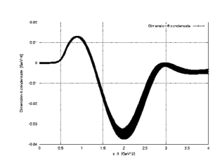
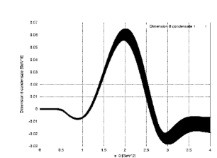
Condensates $\left\langle\mathcal{O}_{6}\right\rangle$ and $\left\langle\mathcal{O}_{8}\right\rangle$ as a function of $s_{0}$. The error bands include the propagation of experimental uncertainties.

Figure 6.4:

Determination of $\left\langle\mathcal{O}_{6}\right\rangle$ and $\left\langle\mathcal{O}_{8}\right\rangle$ using different finite energy sum rules, as described in Ref. [condensates].

Our final determination of the nonperturbative condensates including all relevant sources of uncertainties is

$$\left\langle\mathcal{O}_{6}\right\rangle=\left(-4.0~{}\pm 2.0\right)~{}10^{-3}~{}\mathrm{GeV}^{6}\ ,$$

$$\left\langle\mathcal{O}_{8}\right\rangle=\left(-12~{}\hbox{${\lower 1.0pt\hbox{$\scriptstyle+~{}7$}}\atop{\raise 1.0pt\hbox{$\scriptstyle-~{}11$}}$}\right)10^{-3}~{}\mathrm{GeV}^{8}\ ,$$ (6.16)

$$\left\langle\mathcal{O}_{10}\right\rangle=\left(7.8\pm 2.4\right)~{}10^{-2}~{}\mathrm{GeV}^{10}\ ,$$

$$\left\langle\mathcal{O}_{12}\right\rangle=\left(-2.6\pm 0.8\right)~{}10^{-1}~{}\mathrm{GeV}^{12}\ .$$ (6.17)

The values of the QCD nonperturbative condensates have been previously extracted from the experimental data, with different techniques and different results, as summarized in Table 6.3. We include also the results of works which were published after the original publication of Ref. [condensates]. Note that our results agree, at least on the sign, with that of Refs. [prades, cirigliano, sumrules, cirigliano2, valencia]. See [friot, narisoncon] for a detailed comparison of the different methods for the extraction of the condensates.

Reference	$\left\langle\mathcal{O}_{6}\right\rangle\times 10^{3}~{}\mathrm{GeV}^{6}$	$\left\langle\mathcal{O}_{8}\right\rangle\times 10^{3}~{}\mathrm{GeV}^{8}$
Ref. [davier]	$-6.4\pm 1.6$	$8.7\pm 2.4$
Ref. [ioffe]	$-6.8\pm 2.1$	$7\pm 4$
Ref. [prades]	$-3.2\pm 2.0$	$-12.4\pm 9.0$
Ref. [periscond]	$-9.5\pm 3$	$16.2\pm 5$
Ref. [cirigliano]	$-4.45\pm 0.7$	$-6.2\pm 3.2$
Ref. [sumrules]	$-4\pm 1$	$-1.2\pm 6$
Ref. [condensates] (This work)	$-4\pm 2$	$-12~{}\hbox{${\lower 1.0pt\hbox{$\scriptstyle+~{}7$}}\atop{\raise 1.0pt\hbox{$\scriptstyle-~{}11$}}$}$
Ref. [zyabluk]	$-7.2\pm 1.2$	$7.8\pm 2.5$
Ref. [friot]	$-7.9\pm 1.6$	$11.7\pm 2.7$
Ref. [narisoncon]	$-8.7\pm 2.3$	$15.6\pm 4.0$
Ref. [valencia]	$-2.3\pm 0.5$	$-5\pm 3$

Table 6.3:

Summary of different extractions of the QCD vacuum condensates. Appropriate rescaling have been performed to allow the comparison of different determinations. Note that some of the above determinations appeared after the original publication of Ref. [condensates].

Since the work presented in Ref. [condensates] was published, there have appeared several studies which also determine the values of the higher dimensional condensates from experimental data using a wide variety of methods and techniques [zyabluk, friot, narisoncon, ioffe, cata, physicstau, valencia, string], from large $N_{C}$ methods to new sum rule approaches and even a determination inspired in higher dimensional string theories. The spread of the results obtained for the higher dimensional vacuum condensates using different techniques show that their determination from experimental data is still an open issue.

Summarizing, in this part of the thesis we have presented a determination a bias-free neural network parametrization of the $\rho_{V-A}(s)$ spectral function, inferred from the data, which retains all the information on experimental errors and correlations, and is supplemented with the additional theoretical input of the chiral sum rules. As a byproduct of this analysis, we have performed an extraction of the nonperturbative vacuum condensates $\left\langle\mathcal{O}_{6}\right\rangle$ and $\left\langle\mathcal{O}_{8}\right\rangle$ aimed at minimizing the sources of theoretical bias which might be cause of concern in existing determinations of these condensates from spectral functions. Our final results give negative central values for the dimension 6 and 8 condensates. These results take into account the propagation of statistical errors and their correlations. Higher dimension condensates carry larger errors, although the sign of the condensates seem to remain unaltered.

6.2 Structure functions in deep inelastic scattering

As has been discussed in the Introduction and in Section 4.1.2, the requirements of precision physics at hadron colliders have recently led to a rapid improvement in the techniques for the determination of parton distributions of the nucleon, which are mostly extracted from deep-inelastic structure functions [pdfs]. Specifically, it is now mandatory to determine accurately the uncertainty on these quantities. The main problem to be faced here is that one is trying to determine the uncertainty on a function, i.e., a probability measure on a space of functions, and to extract it from a finite set of experimental data. In Ref. [f2ns] this problem was studied in a simpler context, namely, the determination of a structure function and associate error from the pertinent data. This sidesteps the technical complication of extracting parton distributions from structure functions, but it does tackle the main issue, namely the determination of an error on a function. Furthermore, the determination of a structure function and associate error might be useful for a variety of applications, such as precision tests of QCD (determination of $\alpha_{s}$ [alphas], tests of sum rules) or the determination of polarized structure functions from asymmetry data [smc].

In this part of the thesis we extend the results of Ref. [f2ns] by constructing a parametrization of the proton $F_{2}(x,Q^{2})$ structure function which includes all available data, in particular the HERA collider data. Besides the obvious motivation of having state-of-the art results for this quantity, the main aim of this work is to develop a set of techniques which are required for the application of the method of Ref. [f2ns] to cases where the handling of a large number of disparate data sets is required. A more detailed description of this part of the thesis can be found in the original work, Ref. [f2nnp].

Figure 6.5: Kinematic range of the available experimental data for the proton structure function $F_{2}^{p}(x,Q^{2})$.

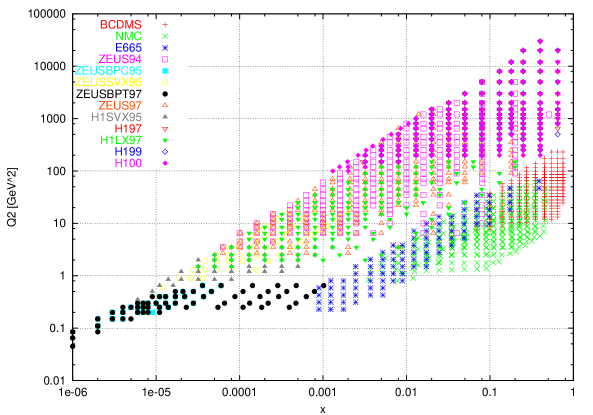
Therefore, we construct a parametrization of the $F_{2}(x,Q^{2})$ structure function based on all available unpolarized charged lepton-proton deep-inelastic scattering data. However, we do not include early SLAC data, for which the covariance matrix is not available, since they do not provide any extra kinematic coverage, and are anyway less precise than later data. This leaves a total of 13 experiments, listed in Table 6.4, along with their main features. Note that the averages of the different types of uncertainties are given in percentage. The coverage of the $(x,Q^{2})$ kinematic plane afforded by these data is shown in Fig. 6.5. Note that the kinematical coverage of the experimental data included in the present parametrization span 6 orders of magnitude in both $x$ and $Q^{2}$.

As has been discussed in Section 4.1.2, deep-inelastic structure functions are defined by parametrizing the deep-inelastic neutral current scattering cross section as

$$\frac{d^{2}\sigma}{dxdQ^{2}}=\frac{4\pi\alpha^{2}}{xQ^{4}}\left[xy^{2}F_{1}(x,Q^{2})+(1-y)F_{2}(x,Q^{2})+y\left(1-\frac{y}{2}\right)F_{3}(x,Q^{2})\right]\ .$$ (6.18)

We will construct a parametrization of the structure function $F_{2}(x,Q^{2})$, which provides the bulk of the contribution to Eq. 6.18. In fact, a large number of experiments present their results in terms of the reduced cross section,

$$\tilde{\sigma}(x,Q^{2})\equiv\frac{xQ^{4}}{4\pi\alpha^{2}\left(1+(1-y)^{2}\right)}\frac{d^{2}\sigma(x,Q^{2})}{dxdQ^{2}}\ ,$$ (6.19)

which is equal to $F_{2}(x,Q^{2})$ in most of the $(x,Q^{2})$ kinematical range. For all experiments the longitudinal structure function $F_{L}(x,Q^{2})$ contribution, defined as

$$F_{L}(x,Q^{2})=\left(1+\frac{4M^{2}x^{2}}{Q^{2}}\right)F_{2}(x,Q^{2})-2xF_{1}(x,Q^{2})\ ,$$ (6.20)

to the cross section has already been subtracted by the experimental collaborations, except for ZEUSBPC95, where we subtracted it using the values published by the same experiment. Note that the structure function $F_{2}$ receives contributions from both $\gamma$ and $Z$ exchange, though the $Z$ contribution is only non-negligible for the high $Q^{2}$ datasets ZEUS94, H197, H199 and H100. We will construct a parametrization of the structure function $F_{2}$ defined in Eq. 6.18, i.e. containing all contributions, since it is closer to the quantity which is experimentally measured, the reduced cross section Eq. 6.19. When the experimental collaborations provide separately the contributions to $F_{2}$ due to $\gamma$ or $Z$ exchange we have recombined them in order to get the full $F_{2}$ Eq. 6.18.

Experiment	Ref.	$x$ range	$Q^{2}$ range	$N_{\mathrm{dat}}$	$\left\langle\sigma_{\mathrm{stat}}\right\rangle$	$\left\langle\sigma_{\mathrm{sys}}\right\rangle$	$\left\langle\frac{\sigma_{\mathrm{sys}}}{\sigma_{\mathrm{stat}}}\right\rangle$	$\left\langle\sigma_{N}\right\rangle$	$\left\langle\sigma_{tot}\right\rangle$	$\left\langle\rho\right\rangle$	$\left\langle\mathrm{cov}\right\rangle$
NMC	[nmc]	$2.0~{}10^{-3}~{}-~{}6.0~{}10^{-1}$	$0.5-75$	288	3.7	2.3	0.76	2.0	5.0	0.17	3.8
BCDMS	[bcdms1, bcdms2]	$6.0~{}10^{-2}~{}-~{}8.0~{}10^{-1}$	$7-260$	351	3.2	2.0	0.56	3.0	5.4	0.52	13.1
E665	[e665]	$8.0~{}10^{-4}~{}-~{}6.0~{}10^{-1}$	$0.2-75$	91	8.7	5.2	0.67	2.0	11.0	0.21	21.7
ZEUS94	[ZEUS94]	$6.3~{}10^{-5}~{}-~{}5.0~{}10^{-1}$	$3.5-5000$	188	7.9	3.5	1.04	2.0	10.2	0.12	6.4
ZEUSBPC95	[ZEUSBPC95]	$2.0~{}10^{-6}~{}-~{}6.0~{}10^{-5}$	$0.11-0.65$	34	2.9	6.6	2.38	2.0	7.6	0.61	34.1
ZEUSSVX95	[ZEUSSVX95]	$1.2~{}10^{-5}~{}-~{}1.9~{}10^{-3}$	$0.6-17$	44	3.8	5.7	1.53	1.0	7.1	0.10	4.1
ZEUS97	[ZEUS97]	$6.0~{}10^{-5}~{}-~{}6.5~{}10^{-1}$	$2.7-30000$	240	5.0	3.1	0.93	3.0	6.7	0.29	7.0
ZEUSBPT97	[ZEUSBPT97]	$6.0~{}10^{-7}~{}-~{}1.3~{}10^{-3}$	$0.045-0.65$	70	2.6	3.6	1.40	1.8	4.9	0.41	8.8
H1SVX95	[H1SVX95]	$6.0~{}10^{-6}~{}-~{}1.3~{}10^{-3}$	$0.35-3.5$	44	6.7	4.6	0.74	3.0	8.9	0.36	28.1
H197	[H197]	$3.2~{}10^{-3}~{}-~{}6.5~{}10^{-1}$	$150-30000$	130	12.5	3.2	0.31	1.5	13.3	0.06	10.9
H1LX97	[H1LX97]	$3.0~{}10^{-5}~{}-~{}2.0~{}10^{-1}$	$1.5-150$	133	2.6	2.2	0.87	1.7	3.9	0.30	3.9
H199	[H199]	$2.0~{}10^{-3}~{}-~{}6.5~{}10^{-1}$	$150-30000$	126	14.7	2.8	0.24	1.8	15.2	0.05	11.0
H100	[H100]	$1.3~{}10^{-3}~{}-~{}6.5~{}10^{-1}$	$100-30000$	147	9.4	3.2	0.42	1.8	10.4	0.09	8.6

Table 6.4: Experiments included in this analysis. All values of $\sigma$ and cov are given as percentages.

Experimental data on deep-inelastic structure functions consist on central values, statistical errors, and the contributions from the different sources of correlated and uncorrelated uncertainties. Uncorrelated systematic errors are added in quadrature to the statistical errors to construct the total uncorrelated uncertainty. On top of this, for some experiments, in particular for the ZEUS94, ZEUSSVX95 and ZEUSBPT97 experiments some uncertainties are asymmetric. For the treatment of asymmetric uncertainties we follow the prescription discussed in Section 5.1.1.

The construction of a parametrization of $F_{2}(x,Q^{2})$ according to general strategy described in Chapter 5 consists in three steps: generation of a set of Monte Carlo replicas of the original experimental data, training of a neural network to each replica and finally statistical validation of the constructed probability measure. The Monte Carlo replicas of the original experiment are generated as a multi-gaussian distribution: each replica is given, following Eq. 5.3, by a set of values

$$F_{i}^{(\mathrm{art})(k)}=\left(1+r_{N}^{(k)}\sigma_{N}\right)\left(F_{i}^{\rm(\mathrm{exp})}+\sum_{l=1}^{N_{\mathrm{sys}}}r_{\mathrm{sys},li}^{(k)}\sigma_{\mathrm{sys},li}+r_{t,i}^{(k)}\sigma_{t,i}\right)\ ,\qquad k=1,\ldots,N_{\mathrm{rep}}\ ,$$ (6.21)

where the various errors are defined in Eqns. 5.4-5.8. As has been discussed before, the value of $N_{\mathrm{rep}}$ is determined in such a way that the Monte Carlo set of replicas models faithfully the probability distribution of the data in the original set. A comparison of expectation values, variances and correlations of the Monte Carlo set with the corresponding input experimental values as a function of the number of replicas is shown in Fig. 6.6, where we display scatter plots of the central values and errors for samples of 10, 100 and 1000 replicas. The corresponding plot for correlations is essentially the same as that shown in Ref. [f2ns]. A more quantitative comparison is performed using the statistical estimators as defined in Section 5.1. The results for these estimators are presented in Table 6.5. Note in particular the scatter correlations $r$ for central values, errors and correlations, which indicate the size of the spread of data around a straight line. The table shows that a sample of 1000 replicas is sufficient to ensure average scatter correlations of 99% and accuracies of a few percent on structure functions, errors and correlations.

$F_{2}^{p}(x,Q^{2})$
$N_{\mathrm{rep}}$	10	100	1000
$\left\langle PE\left[\left\langle F^{(\mathrm{art})}\right\rangle_{\mathrm{rep}}\right]\right\rangle$	1.88%	0.64%	0.20%
$r\left[F^{(\mathrm{art})}\right]$	0.99919	0.99992	0.99999
$\left\langle V\left[\sigma^{(\mathrm{art})}\right]\right\rangle_{\mathrm{dat}}$	$6.7\times 10^{-4}$	$2.0\times 10^{-4}$	$6.9\times 10^{-5}$
$\left\langle PE\left[\sigma^{(\mathrm{art})}\right]\right\rangle_{\mathrm{dat}}$	37.21%	11.77%	3.43%
$\left\langle\sigma^{(\mathrm{art})}\right\rangle_{\mathrm{dat}}$	0.0292	0.0317	0.0316
$r\left[\sigma^{(\mathrm{art})}\right]$	0.945	0.995	0.999
$\left\langle V\left[\rho^{(\mathrm{art})}\right]\right\rangle_{\mathrm{dat}}$	$8.1\times 10^{-2}$	$7.8\times 10^{-3}$	$7.3\times 10^{-4}$
$\left\langle\rho^{(\mathrm{art})}\right\rangle_{\mathrm{dat}}$	0.3048	0.3115	0.2920
$r\left[\rho^{(\mathrm{art})}\right]$	0.696	0.951	0.995
$\left\langle V\left[\mathrm{cov}^{(\mathrm{art})}\right]\right\rangle_{\mathrm{dat}}$	$5.2\times 10^{-7}$	$6.8\times 10^{-8}$	$6.9\times 10^{-9}$
$\left\langle\mathrm{cov}^{(\mathrm{art})}\right\rangle_{\mathrm{dat}}$	0.00013	0.00018	0.00015
$r\left[\mathrm{cov}^{(\mathrm{art})}\right]$	0.687	0.941	0.994

Table 6.5: Comparison between experimental and Monte Carlo data. The experimental data have $\left\langle\sigma^{(\mathrm{exp})}\right\rangle_{\mathrm{dat}}=0.0311$, $\left\langle\rho^{(\mathrm{exp})}\right\rangle_{\mathrm{dat}}=0.2914$ and $\left\langle\mathrm{cov}^{(\mathrm{exp})}\right\rangle_{\mathrm{dat}}=0.00015$. All statistical indicators are defined in Section 5.1.

Figure 6.6: Scatter plot of experimental data versus Monte Carlo artifical data for both central values and errors.

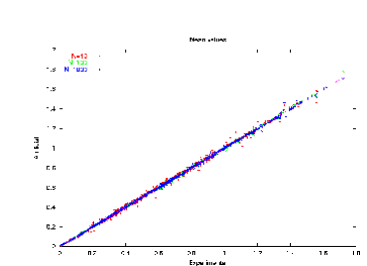
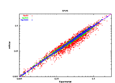
$N_{\mathrm{rep}}$ neural networks are then trained on the Monte Carlo replicas, by training each neural network on all the $F_{i}^{(k)(\mathrm{art})}$ data points in the $k$-th replica. The architecture of the networks is the same as in Ref. [f2ns]. The training is subdivided in three epochs, each based on the minimization of a different error function, as described in Section 5.2.3. First one minimizes $E_{1}^{(k)}$, then $E_{2}^{(k)}$ and finally correlated systematics are incorporated in the minimization of $E_{3}^{(k)}$. The rationale behind this three-step procedure is that the true minimum which the fitting procedure must determine is that of the error function with correlated systematics $E_{3}^{(k)}$ Eq. 5.34. However, this is nonlocal and time consuming to compute. It is therefore advantageous to look for its rough features at first, then refine its search, and finally determine its actual location.

The minimum during the first two epochs is found using back-propagation (BP), discussed in Section 5.2.3. This method is not suitable for the minimization of the nonlocal function Eq. 5.34. In Ref. [f2ns] BP was used throughout, and the third epoch was omitted. This is acceptable provided the total systematics is small in comparison to the statistical errors, and indeed it was verified that a good approximation to the minimum of Eq. 5.34 could be obtained from the ensemble of neural networks. This is no longer the case for the present extended data set, as we shall see explicitly in brief. Therefore, the full $E_{3}^{(k)}$ Eq. 5.34 is minimized in the third training epoch by means of genetic algorithms (GA), also discussed in Section 5.2.3.

At the end of the GA training we are left with a sample of $N_{\mathrm{rep}}$ neural networks, from which e.g. the value of the structure function at $(x,Q^{2})$ can be computed as

$$F_{2}(x,Q^{2})=\frac{1}{N_{\mathrm{rep}}}\sum_{k=1}^{N_{\mathrm{rep}}}F^{(\mathrm{net})(k)}(x,Q^{2})\ .$$ (6.22)

The goodness of fit of the final set is thus measured by the $\chi^{2}$ per data point, Eq. 5.76, which, given the large number of data points is essentially identical to the $\chi^{2}$ per degree of freedom.

In order to apply the general strategy to the present problem several points must be considered: the choice of training parameters and training length, the choice of the actual data set, and the choice of theoretical constraints. We now address these issues in turn. The parameters and length for the first two training epochs have been determined by inspection of the fit of a neural network to the central experimental values. Clearly, this choice is less critical, in that it is only important in order for the training to be reasonably fast, but it does not impact on final result.

After these first two training epochs, the diagonal error function $E_{2}^{(0)}$, Eq. 5.33, for a training on central values is of order two for the central data set, with a similar length of the training than that that was required to reach $E_{2}^{(0)}\approx 1.3$ for the smaller data set of Ref. [f2ns]. The value of $E_{3}^{(0)}$, Eq. 5.34, which is always bounded by it, $E_{3}\leq E_{2}$ is accordingly smaller (see Table 6.6). The training algorithm then switches to GA minimization of the $E_{3}$, Eq. 5.34. The determination of the length of this training epoch is critical, in that it controls the form of the final fit. This can only be done by looking at the features of the full Monte Carlo sample of neural networks.

TABLE 3
	A		B
Experiment	$E_{2}$	$E_{3}$	$E_{2}$	$E_{3}$
Total	2.05	1.54	2.03	1.36
NMC	1.97	1.56	1.74	1.54
BCDMS	1.93	1.66	1.32	1.26
E665	1.64	1.37	1.83	1.38
ZEUS94	3.15	2.26	3.01	2.21
ZEUSBPC95	4.18	1.32	5.18	1.24
ZEUSSVX95	3.37	1.88	5.68	2.11
ZEUS97	2.33	1.54	3.02	1.37
ZEUSBPT97	2.82	1.97	2.08	1.22
H1SVX95	3.21	0.96	4.74	1.09
H197	0.86	0.76	1.08	0.87
H1LX97	1.96	1.46	1.50	1.18
H199	1.15	1.07	1.10	1.01
H100	1.59	1.50	1.48	1.26

Table 6.6: The uncorrelated error function, $E_{2}^{(0)}$, Eq. 5.33, and the correlated one, $E_{3}^{(0)}$, Eq. 5.34, for the fit to the central data points: (A) after the back-propagation training epoch and (B) after the final genetic algorithms training epoch.

Before addressing this issue, however, it turns out to be necessary to consider the possibility of introducing cuts in the data set. Indeed, consider the results obtained after a GA training of $4\times 10^{4}$ generation to the central data set, displayed in Table 6.6. This is a rather long training: indeed, in each GA generation all the data are shown to the nets. Hence in $4\times 10^{4}$ GA generations the data are shown to the nets $0.7\times 10^{8}$ times, comparable to the number of times they are shown to the nets during BP training. It is apparent that whereas $E_{3}\sim 1$ for most experiments, it remains abnormally high for NMC and especially ZEUS94 and ZEUSSVX95. Because of the weighted training which has been adopted, this is unlikely to be due to insufficient training of these data sets, and is more likely related to problems of these data sets.

Whereas ZEUSSVX95 only contains a small number of data points, NMC and ZEUS94 account each for more than 10% of the total number of data points, and thus they can bias final results considerably. The case of NMC was discussed in detail in Ref. [f2ns]. This data set is the only one to cover the medium-$x$, medium-small $Q^{2}$ region (see Fig. 6.5) and thus it cannot be excluded from the fit. As discussed in Ref. [f2ns], the relatively large value of $E_{3}$ for this experiment is a consequence of internal inconsistencies within the data set. A value of $E_{3}\approx 1.5$ indicates that the neural nets do not reproduce the subset of data which are incompatible with the bulk, as it should be, whereas a value $E_{3}\approx 1$ could only be obtained by overlearning, i.e. essentially by fitting irrelevant fluctuations (see Ref. [f2ns]).

Let us now consider the case of ZEUS94. The kinematic region of this experiment is entirely covered by the ZEUS97, H197, H199 and H100 experiments. We can therefore study the impact of excluding this experiment from the global fit, without information loss. The results obtained in such case are displayed in Table 6.7: when the experiment is not fitted the $E_{3}$ value for all experiments with which it overlaps improves and so does the global $E_{3}$, whereas $E_{3}$ for ZEUS94 itself only deteriorates by a comparable amount, despite the fact that the experiment is now not fitted at all. We conclude that the experiment should be excluded from the fit, since its inclusion results in a deterioration of the fit quality, whereas its exclusion does not entail information loss. Difficulties in the inclusion of this experiment in global fits were already pointed out in Refs. [GKK, alekhin], where it was suggested that they may be due to underestimated or non-gaussian uncertainties. It is likely that ZEUSSVX95 has similar problems. However, its inclusion in the fit is no reason of concern, even if its high $E_{3}$ value were due to incompatibility of this experiment with the others or underestimate of its experimental uncertainties, because of the small number of data points. It is therefore retained in the data set. Our final data set thus includes all experiments in Table 6.4, except ZEUS94. We are thus left with $N_{\mathrm{dat}}=$1698 data points.

TABLE 4
Experiment	$E_{3}$
Total	1.25
NMC	1.51
BCDMS	1.24
E665	1.23
ZEUS94	2.28
ZEUSBPC95	1.16
ZEUSSVX95	2.08
ZEUS97	1.37
ZEUSBPT97	1.00
H1SVX95	1.04
H197	0.84
H1LX97	1.19
H199	1.00
H100	1.24

Table 6.7: The same fit as the last column of Table 6.6 if the ZEUS94 data are excluded from the fit.

For the sake of future applications, it is interesting to ask how the procedure of selecting experiments in the data set can be automatized. This can be done in an iterative way as follows: first, a neural net (or sample of neural nets) is trained on only one experiment; then, the total $E_{3}$ for the full data set is computed using this neural net (or sample of nets); the procedure is then repeated for all experiments, and the experiment which leads to the smallest total $E_{3}$ is selected. In the second iteration, the net (or sample of nets) is trained on the experiment selected in the first iteration plus any of the other experiments, thereby leading to the selection of a second experiment to be added to that selected previously, and so on. The process can be terminated before all experiments are selected, for instance if it is seen that the addition of a new experiment does not lead to a significant improvement in $E_{3}$ for a large enough length of training.

Figure 6.7: Dependence of the total $\chi^{2}$ Eq. 5.76 on the length of training: (left) total training (right) detail of the GA training.

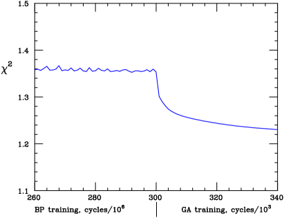
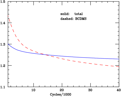
We now proceed to discuss the length of training for our final data set. The total $\chi^{2}$, Eq. 5.76, as computed from averages over the trained network sample, is shown in Fig. 6.7 as a function of the number of GA generations. The $\chi^{2}$ decreases very rapidly during the first few hundreds of training generations, a typical feature of genetic algorithms minimization. After about 5000 training generations, the $\chi^{2}$ as a function of the training length essentially flattens for all experiments but BCDMS. The further decrease of the total $\chi^{2}$ is then due essentially to the decrease of the contribution from BCDMS. A training length of $4\times 10^{4}$ GA generations is necessary in order for the $\chi^{2}$ of BCDMS to flatten out at $\chi^{2}\sim 1.2$. As discussed in Ref. [f2ns], the BCDMS data can only be learnt with a longer training because they have high precision while being located in the intermediate $x$ (valence) region, where the parton distributions display significant variation.

The $E_{3}^{(0)}$ values for the fit of a neural net to the central data with this training is given in Table 6.6. It shows that all experiments are well reproduced with the exceptions discussed above. It is interesting to observe that while $E_{3}^{(0)}$ Eq. 5.34 decreases significantly during the GA training, the uncorrelated $E_{2}^{(0)}$, Eq. 5.33, decreases marginally, and in fact it actually increases for several HERA experiments. This shows that correlations are sizable for the HERA experiments, so that the approach of Ref. [f2ns], based on the minimization of $E_{2}$, is not adequate in this case. GA minimization appears to be very efficient in reducing the $E_{3}$ value relatively fast.

$F_{2}^{p}(x,Q^{2})$
$N_{\mathrm{rep}}$	1000
$\chi^{2}$	1.18
$\left\langle E\right\rangle$	2.52
$r\left[F^{(\mathrm{net})}\right]$	0.99
${\cal R}$	0.54
$\left\langle V\left[\sigma^{(\mathrm{net})}\right]\right\rangle_{\mathrm{dat}}$	$1.2~{}10^{-3}$
$\left\langle PE\left[\sigma^{(\mathrm{net})}\right]\right\rangle_{\mathrm{dat}}$	$80\%$
$\left\langle\sigma^{(\mathrm{exp})}\right\rangle_{\mathrm{dat}}$	0.027
$\left\langle\sigma^{(\mathrm{net})}\right\rangle_{\mathrm{dat}}$	0.008
$r\left[\sigma^{(\mathrm{net})}\right]$	0.73
$\left\langle V\left[\rho^{(\mathrm{net})}\right]\right\rangle_{\mathrm{dat}}$	0.20
$\left\langle\rho^{(\mathrm{exp})}\right\rangle_{\mathrm{dat}}$	0.31
$\left\langle\rho^{(\mathrm{net})}\right\rangle_{\mathrm{dat}}$	0.67
$r\left[\rho^{(\mathrm{net})}\right]$	0.54
$\left\langle V\left[\mathrm{cov}^{(\mathrm{art})}\right]\right\rangle_{\mathrm{dat}}$	$3.3~{}10^{-7}$
$\left\langle\mathrm{cov}^{(\mathrm{exp})}\right\rangle_{\mathrm{dat}}$	$1.3~{}10^{-4}$
$\left\langle\mathrm{cov}^{(\mathrm{net})}\right\rangle_{\mathrm{dat}}$	$3.6~{}10^{-5}$
$r\left[\mathrm{cov}^{(\mathrm{net})}\right]$	0.49

Table 6.8:

Estimators of the final results for the constructed probability measure of $F_{2}(x,Q^{2})$.

Experiment	NMC	BCDMS	E665
$\chi^{2}$	1.47	1.19	1.20
$\left\langle E\right\rangle$	2.69	3.17	2.29
$r\left[F^{(\mathrm{net})}\right]$	0.96	0.99	0.91
${\cal R}$	0.59	0.50	0.56
$\left\langle V\left[\sigma^{(\mathrm{net})}\right]\right\rangle_{\mathrm{dat}}$	$0.002$	$1.9~{}10^{-5}$	0.0013
$\left\langle PE\left[\sigma^{(\mathrm{net})}\right]\right\rangle_{\mathrm{dat}}$	0.63	0.56	0.89
$\left\langle\sigma^{(\mathrm{exp})}\right\rangle_{\mathrm{dat}}$	0.017	0.007	0.032
$\left\langle\sigma^{(\mathrm{net})}\right\rangle_{\mathrm{dat}}$	0.008	0.005	0.008
$r\left[\sigma^{(\mathrm{net})}\right]$	0.23	0.98	0.17
$\left\langle V\left[\rho^{(\mathrm{net})}\right]\right\rangle_{\mathrm{dat}}$	0.51	0.69	0.29
$\left\langle\rho^{(\mathrm{exp})}\right\rangle_{\mathrm{dat}}$	0.17	0.52	0.20
$\left\langle\rho^{(\mathrm{net})}\right\rangle_{\mathrm{dat}}$	0.84	0.86	0.60
$r\left[\rho^{(\mathrm{net})}\right]$	0.08	0.73	0.05
$\left\langle V\left[\mathrm{cov}^{(\mathrm{art})}\right]\right\rangle_{\mathrm{dat}}$	$2.4~{}10^{-9}$	$1.8~{}10^{-9}$	$4.5~{}10^{-9}$
$\left\langle\mathrm{cov}^{(\mathrm{exp})}\right\rangle_{\mathrm{dat}}$	$4.4~{}10^{-5}$	$3.8~{}10^{-5}$	$1.7~{}10^{-4}$
$\left\langle\mathrm{cov}^{(\mathrm{net})}\right\rangle_{\mathrm{dat}}$	$5.2~{}10^{-5}$	$2.3~{}10^{-5}$	$3.3~{}10^{-5}$
$r\left[\mathrm{cov}^{(\mathrm{net})}\right]$	-0.03	0.98	0.16

Experiment	ZEUSBPC95	ZEUSSVX95	ZEUS97	ZEUSBPT97	H1SVX95	H197	H1LX97	H199	H100
$\chi^{2}$	1.02	2.08	1.35	0.86	0.67	0.71	1.07	0.90	1.11
$\left\langle E\right\rangle$	2.07	2.03	2.24	2.08	2.03	1.91	2.41	1.93	2.11
$r\left[F^{(\mathrm{net})}\right]$	0.98	0.96	0.99	0.99	0.97	0.99	0.99	0.98	0.99
${\cal R}$	0.51	0.66	0.55	0.55	0.44	0.46	0.53	0.48	0.54
$\left\langle V\left[\sigma^{(\mathrm{net})}\right]\right\rangle_{\mathrm{dat}}$	$4.3~{}10^{-4}$	0.0035	0.0010	$1.3~{}10^{-4}$	0.0043	0.0030	0.0005	0.003	0.0013
$\left\langle PE\left[\sigma^{(\mathrm{net})}\right]\right\rangle_{\mathrm{dat}}$	0.91	0.94	0.87	0.72	0.96	0.95	0.75	0.96	0.93
$\left\langle\sigma^{(\mathrm{exp})}\right\rangle_{\mathrm{dat}}$	0.022	0.061	0.037	0.012	0.063	0.040	0.027	0.051	0.030
$\left\langle\sigma^{(\mathrm{net})}\right\rangle_{\mathrm{dat}}$	0.006	0.013	0.011	0.006	0.011	0.008	0.008	0.008	0.009
$r\left[\sigma^{(\mathrm{net})}\right]$	0.85	0.72	0.86	0.73	0.84	0.87	0.42	0.82	0.89
$\left\langle V\left[\rho^{(\mathrm{net})}\right]\right\rangle_{\mathrm{dat}}$	0.09	0.30	0.12	0.14	0.118	0.14	0.31	0.16	0.14
$\left\langle\rho^{(\mathrm{exp})}\right\rangle_{\mathrm{dat}}$	0.61	0.24	0.28	0.40	0.36	0.06	0.29	0.05	0.09
$\left\langle\rho^{(\mathrm{net})}\right\rangle_{\mathrm{dat}}$	0.77	0.64	0.39	0.63	0.57	0.27	0.58	0.29	0.26
$r\left[\rho^{(\mathrm{net})}\right]$	0.53	0.40	0.66	0.60	0.48	0.51	0.69	0.37	0.55
$\left\langle V\left[\mathrm{cov}^{(\mathrm{art})}\right]\right\rangle_{\mathrm{dat}}$	$6.4~{}10^{-8}$	$1.9~{}10^{-6}$	$3.4~{}10^{-7}$	$1.4~{}10^{-9}$	$3.0~{}10^{-6}$	$3.8~{}10^{-7}$	$3.8~{}10^{-8}$	$2.7~{}10^{-7}$	$1.7~{}10^{-7}$
$\left\langle\mathrm{cov}^{(\mathrm{exp})}\right\rangle_{\mathrm{dat}}$	$2.8~{}10^{-4}$	$8.5~{}10^{-4}$	$3.7~{}10^{-4}$	$5.8~{}10^{-5}$	0.0014	$1.0~{}10^{-4}$	$2.1~{}10^{-4}$	$1.4~{}10^{-4}$	$9.6~{}10^{-5}$
$\left\langle\mathrm{cov}^{(\mathrm{net})}\right\rangle_{\mathrm{dat}}$	$2.8~{}10^{-5}$	$1.2~{}10^{-4}$	$3.2~{}10^{-5}$	$2.3~{}10^{-5}$	$7.0~{}10^{-5}$	$1.510^{-5}$	$6.9~{}10^{-5}$	$1.6~{}10^{-5}$	$2.2~{}10^{-5}$
$r\left[\mathrm{cov}^{(\mathrm{net})}\right]$	0.69	0.48	0.77	0.65	0.53	0.61	0.57	0.54	0.58

Table 6.9: Final results for the individual experiments: fixed target (top) and HERA (bottom)

We finally turn to the issue of theoretical constraints. The only theoretical assumption on the shape of $F_{2}(x,Q^{2})$ is that it satisfies the kinematic constraint $F_{2}(1,Q^{2})=0$ for all $Q^{2}$. As this constraint is local, its implementation is straightforward: it can be enforced by including in the data set a number of artificial data points which satisfy the constraint with a suitably tuned error. In the present fit we have checked that the best choice is to add a number of artificial points at $x=1$, as discussed in Section 5.2.4, equal to 2% of the experimental trained points (33 points with ZEUS94 excluded from the fits), and with error equal to one tenth of the mean statistical error of the trained points. These points are equally spaced in $\ln Q^{2}$, within the range covered by the experimental data.

The result of the minimization of a single neural net to the central data points is shown in Table 6.7. The results for the final set of 1000 neural networks are displayed in Table 6.8, while in Table 6.9 we give the details of results for each experiment. Note that the figure of merit for the minimization $E_{3}$, Eq. 5.34, and its average, defined by Eq. 5.77, differs from the full $\chi^{2}$, Eq. 5.76, not only because the latter is computed from the structure function averaged over nets Eq. 6.22, but also because of the different treatment of normalization errors in the respective covariance matrices, Eq. 5.35 and Eq. 5.6. Besides the $\chi^{2}$ we also list the values of various quantities, defined in Section 5.3, which can be used to assess the goodness of fit.

The quality of the final fit is somewhat better than that of the fit to the central data points shown in Table 6.7. In particular, with the exception of NMC (which is likely to have internal inconsistencies [f2ns]) and ZEUSSVX95 (which is likely to have the same problems as those of ZEUS94) the $\chi^{2}$ per degree of freedom is of order 1 for all experiments. It is interesting to note that the $\chi^{2}$ for the neural network average is rather better than the average $\langle E_{3}\rangle$. The (scatter) correlation between experimental data and the neural network prediction equals one to about 1% accuracy, with the exception of NMC, ZEUSSVX95 (which have the aforementioned problems) and E665. The E665 kinematic region overlaps almost entirely (apart from very small $Q^{2}<1$ GeV${}^{2}$) with that of NMC and BCDMS, while having lower accuracy (this is why the experiment was not included in the fits of Ref. [f2ns]). The data points corresponding to this experiment are therefore essentially predicted by the fit to other experiments, thus explaining the somewhat smaller scatter correlation.

The average neural network variance is in general substantially smaller than the average experimental error, typically by a factor $3-4$. This is the reason why $\left\langle E\right\rangle>\chi^{2}$: the neural nets fluctuate less about central experimental values than the Monte Carlo replicas. In the presence of substantial error reduction, the (scatter) correlation between network covariance and experimental error is generally not very high, and can take low values when a small number of data points from one experiment is enough to determine the outcome of the fit, such as in the case of the NMC experiment, even more so for E665 [f2ns].

Figure 6.8:

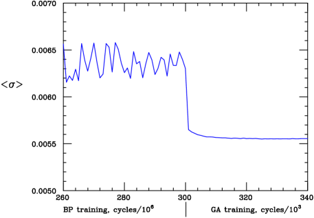
Dependence of $\left\langle\sigma^{(\mathrm{net})}\right\rangle_{\mathrm{dat}}$ on the length of training for the BCDMS experiment.

Figure 6.9:

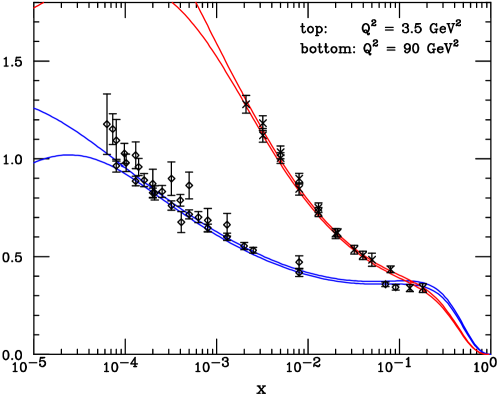
Final results for $F_{2}(x,Q^{2})$ compared to experimental data. For the neural network result, the one-$\sigma$ error band is shown.

As discussed extensively in Ref. [f2ns] it is important to make sure that this is due to the fact that information from individual data points is combined through an underlying law by the neural networks, and not due to parametrization bias. To this purpose, the ${\cal R}$-estimator has been introduced in Section 5.3, where it was shown that in the presence of substantial error reduction ${\cal R}\mathrel{\hbox to0.0pt{\lower 4.0pt\hbox{\hskip 1.0pt$\sim$}\hss}\raise 1.0pt\hbox{$>$}}1$ if there is parametrization bias, whereas ${\cal R}\approx 0.5$ in the absence of parametrization bias. It is apparent from Tables 6.8 and 6.9 that indeed ${\cal R}\approx 0.5$ for all experiments. Note that, contrary to what was found in ref. [f2ns], there is now some error reduction also for the BCDMS experiment, though by a somewhat smaller amount than for other experiments. We will come back to this issue when comparing results to those of Ref. [f2ns].

Further evidence that the error reduction is not due to parametrization bias can be obtained by studying the dependence of $\left\langle\sigma^{(\mathrm{net})}\right\rangle_{\mathrm{dat}}$ on the length of training. This dependence is shown in Fig. 6.8 for the BCDMS experiment. It is apparent that the error reduction is correlated with the goodness of fit displayed in Fig. 6.7, and it occurs during the GA training, thereby suggesting that error reduction occurs when the neural networks start reproducing an underlying law. If error reduction were due to parametrization bias it would be essentially independent of the length of training.

The point-to-point correlation $\rho$ of the neural nets is somewhat larger than that of the data, as one might expect as a consequence of an underlying law which is being learnt by the neural networks. In fact, for the NMC experiment the increase in correlation essentially compensates the reduction in error, in such a way that the average covariance of the nets and the data are essentially the same. This again shows that in the case of the NMC experiment a small number of points is sufficient to predict the remaining ones. For all other experiments, however, the covariance of the nets is substantially smaller than that of the data. As a consequence the (scatter) correlation of covariance remains relatively high for all experiments, except NMC, and especially E665 whose points are essentially predicted by the fit to other experiments.

Figure 6.10:

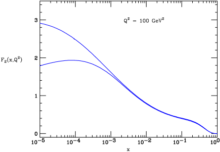
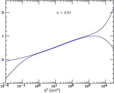
One-$\sigma$ error band for the structure function $F_{2}(x,Q^{2})$ computed from neural nets. Note the different scale on the $y$ axis in the two plots.

The structure function and associated one-$\sigma$ error band is compared to the data as a function of $x$ for a pair of typical values of $Q^{2}$ in Fig. 6.9. In Fig. 6.10 the behavior of the structure function as a function of $x$ at fixed $Q^{2}$ and as a function of $Q^{2}$ at fixed $x$ is also shown. It is apparent that in the data region the error on the neural nets is rather smaller than that on the data used to train them. The error however grows rapidly as soon as the nets are extrapolated outside the region of the data, specially in the small-$x$ region and in the large-$Q^{2}$ region. At large $x$, however, the extrapolation is kept under control by the kinematic constraint $F_{2}(1,Q^{2})=0$. Note that the increase of the uncertainties in the extrapolation region, as opposed to the case for fits with functional forms, is due to the fact that the behavior of neural networks in this region is not determined by the corresponding behavior in the data (interpolation) region.

Figure 6.11:

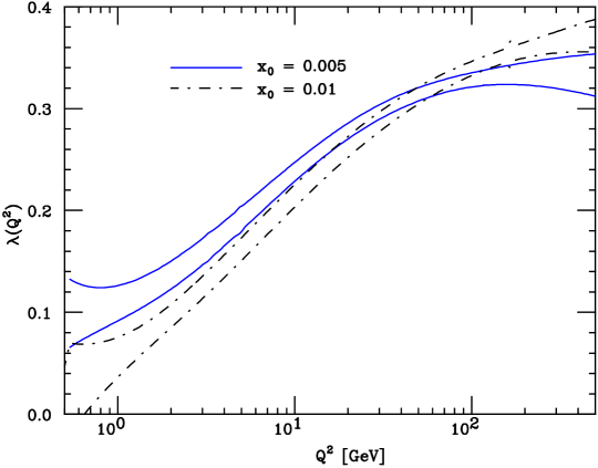
The logarithmic derivative of $F_{2}(x,Q^{2})$, $\lambda(Q^{2})$, as determined from the neural network parametrization in the transition region between perturbative and nonperturbative regimes.

Figure 6.12:

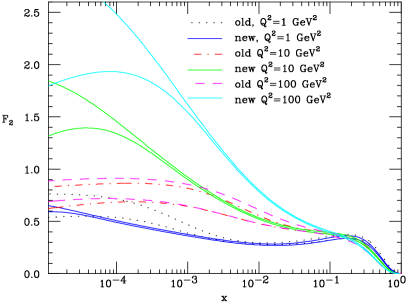
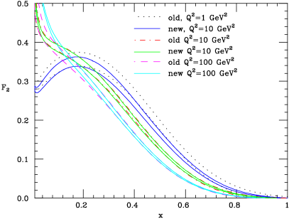
Comparison of the parametrization of $F_{2}(x,Q^{2})$ of ref. [f2ns] (old) with that described in [f2nnp] (new). The pairs of curves correspond to a one-$\sigma$ error band.

The number of possible phenomenological applications of the neural network parametrization of the proton structure function $F_{2}^{p}(x,Q^{2})$ is rather large, from determinations of the strong coupling $\alpha_{s}\left(Q^{2}\right)$, comparison of different theoretical predictions at low $x$, checks of sum rules, or its effects of the extraction of polarized structure functions and polarized parton distributions. Another possibility is a detailed quantitative study of $F_{2}^{p}(x,Q^{2})$ in the transition region between perturbative and nonperturbative regimes around $Q^{2}=1$ GeV${}^{2}$. Our parametrization is specially suited for this purpose since it incorporates all the information from experimental data without introducing any bias from the functional form behavior of the transition region. In Fig. 6.11 we show the logarithmic derivative of the structure function, defined as

$$\lambda(Q^{2},x_{0})\equiv\frac{\ln F_{2}(x,Q^{2})}{d\ln x}\Bigg{|}_{x=x_{0}}\ ,$$ (6.23)

for two different values of $x_{0}$. Note that at very low $Q^{2}$ expectations are that the Pomeron exponent, $\lambda(Q^{2}=0)=0.08$ is recovered.

Let us finally compare the determination of $F_{2}(x,Q^{2})$ presented here with that of Ref. [f2ns], which was based on pre-HERA data. In Fig. 6.12 one-$\sigma$ error bands for the two parametrizations are compared, whereas in Fig. 6.13 we display the relative pull of the two parametrizations, introduced in Section 5.3, which in the present situation is given by

$$P(x,Q^{2})\equiv\frac{F_{2}^{\mathrm{new}}(x,Q^{2})-F_{2}^{\mathrm{old}}(x,Q^{2})}{\sqrt{\sigma_{\mathrm{new}}^{2}(x,Q^{2})+\sigma_{\mathrm{old}}^{2}(x,Q^{2})}}\ ,$$ (6.24)

where $\sigma(x,Q^{2})$ is the error on the structure function determined as the variance of the neural network sample. In view of the fact that the old fit only included BCDMS and NMC data, it is interesting to consider four regions: (a) the BCDMS region (large $x$, intermediate $Q^{2}$, e.g. $x=0.3$, $Q^{2}=20$ GeV${}^{2}$); (b) the NMC region (intermediate $x$, not too large $Q^{2}$, e.g. $x=0.1$, $Q^{2}=2$ GeV${}^{2}$); (c) the HERA region (small $x$ and large $Q^{2}$, e.g. $0.01$ and $Q^{2}>10$ GeV${}^{2}$); (d) the region where neither the old nor the new fit had data (very large or very small $Q^{2}$). In region (a) the new fit is rather more precise than the old one, for reasons to be discussed shortly, while central values agree, with $P\mathrel{\hbox to0.0pt{\lower 4.0pt\hbox{\hskip 1.0pt$\sim$}\hss}\raise 1.0pt\hbox{$<$}}1$). In region (b) the new fit is significantly more precise than the old one, while central values agree to about one sigma. In region (c) the new fit is rather accurate while the old fit had large errors, but $P\gg 1$ nevertheless, because the HERA rise of $F_{2}$ is outside the error bands extrapolated from NMC. This shows that even though errors on extrapolated data grow rapidly they become unreliable when extrapolating far from the data. Finally in region (d) all errors are very large and $P$ is consequently small, except at small $x$ and large $Q^{2}$, where the new fits extrapolate the rise in the HERA data, which is missing altogether in the old fits.

Figure 6.13:

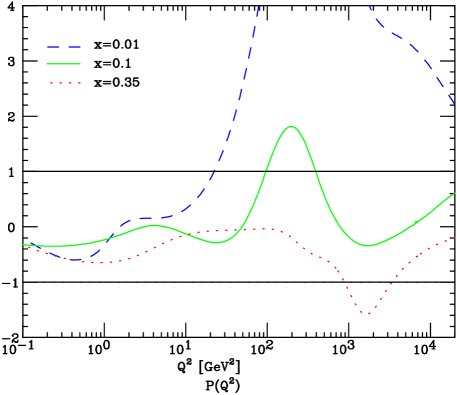
The relative pull, Eq. 6.24, of the new and old $F_{2}(x,Q^{2})$ parametrizations. The one-$\sigma$ band is also shown. Note that in the kinematical region where experimental data for the two versions of the fit overlaps, the pull always verifies $\Big{|}P(x,Q^{2})\Big{|}\leq 1$, as expected from consistency arguments.

Let us finally come to the issue of the BCDMS error, which, as already mentioned, is reduced somewhat in the current fit in comparison to the data and the previous fit. This may appear surprising, in that the new fit does not contain any new data in the BCDMS region. However, as is apparent from Fig. 6.8, this error reduction takes place in the GA training stage, when $E_{3}$ is minimized. Furthermore, we have verified that if the uncorrelated $E_{2}$ is minimized during the GA training no error reduction is observed for BCDMS. Hence, we conclude that the reason why error reduction for BCDMS was not found in Ref. [f2ns] is that in that reference neural networks were trained by minimizing $E_{2}$. In fact, as discussed above, the BCDMS experiment turns out to require the longest time to learn, especially after inclusion of the HERA data. Error reduction only obtains after this lengthy minimization process.

In summary, we have presented a determination of the probability density in the space of structure functions for the structure function $F_{2}(x,Q^{2})$ for the proton, based on all available data from the NMC, BCDMS, E665, ZEUS and H1 collaborations. Our results take the form of a Monte Carlo sample of 1000 neural networks, each of which provides a determination of the structure function for all $(x,Q^{2})$. The structure function and its statistical moments (errors, correlations and so on) can be determined by averaging over this sample. The results of this part of the thesis are made available as a FORTRAN routine which gives $F_{2}(x,Q^{2})$, determined by a set of parameters, and 1000 sets of parameters corresponding to the Monte Carlo sample of structure functions. They can be downloaded from the web site http://sophia.ecm.ub.es/f2neural/.

This works updates and upgrades that of Ref. [f2ns], where similar results were obtained from the BCDMS and NMC data only. The main improvements in the present work are related to the need of handling a large number of experimental data, affected by large correlated systematics. Apart from many smaller technical aspects, the main improvement introduced here is the use of genetic algorithms to train neural networks on top of back-propagation. This has allowed for a more accurate handling of correlated systematics.

Whereas the results of this part of the thesis are of direct practical use for any application where an accurate determination of $F_{2}^{p}(x,Q^{2})$ and its associate error are necessary, its main motivation is the development of a set of techniques which will be required for the construction of a full set of parton distributions with faithful uncertainty estimation based on the same method. The application of this strategy to the parametrization of parton distribution functions is discussed in Section 6.4.

6.3 Lepton energy spectrum in B meson decays

The third application of the general strategy defined in Chapter 5 is the parametrization of the lepton energy distribution from semileptonic decays of B mesons. The motivation for such a parametrization is the application of the general strategy of Chapter 5 to the construction of the probability density of an observable when only its moments are available experimentally. As a byproduct of this parametrization, we will provide a determination of the b quark mass $\overline{m}_{b}\left(m_{b}\right)$.

In the last decade the field of B meson physics has been the object of a wealth of studies (see Ref. [superB] and references therein), motivated by the high precision measurements coming from the B factories Belle and Babar. In particular the inclusive semileptonic decays $B\to Xl\nu$, where $X$ stands for a hadronic system, have received a lot of attention, both in the theoretical and in the experimental sides, due to its paramount importance for the determination of elements of the CKM matrix, and also since they provide us with important information on the underlying strong interaction dynamics.

Therefore, our purpose in this part of the thesis is to allow a more general comparison of the theoretical predictions with the experimental data, constructing a parametrization of the lepton energy spectrum from available experimental information on its moments, supplemented by constraints from the kinematics of the process. This goal is part of a more general motivation, namely the development of a suitable general strategy to determine a function with uncertainties if the only available experimental information is given in terms of its convolutions and additional constraints (like kinematical cuts).

The success of previous applications of the technique introduced in Chapter 5 to other problems motivated us to implement this technique in the context of B physics. Therefore, in this work we construct a unbiased parametrization of the lepton energy spectrum in semileptonic B meson decays with a faithful estimation of the uncertainties.

The semileptonic decays of the B meson have been introduced in Section 4.1.3. We will consider therefore experimental data for leptonic moments with kinematical cuts of the lepton energy distribution, Eq. 4.48, in semileptonic B meson decays to charmed final states $B\to X_{c}l\nu$. These moments have recently been measured with great accuracy at the B-factories, Babar [Aubert:2004td] and Belle [elmombelle], as well as by the Cleo [cleoleptonmom] detector. We will therefore use in the present analysis the latest data from these three experiments. We do not use data from CDF [cdfhadmom] since it is restricted to hadronic moments and leptonic moments are not available. The features of the experimental data of these three experiments can be seen in Table 6.10. Note that for all experiments correlations are rather large, so it is compulsory to incorporate them in a consistent way in the statistical analysis of the data.

Experiment	$N_{\mathrm{dat}}$	$n$	$E_{0}$ (GeV)	$\left\langle\sigma_{\mathrm{stat}}\right\rangle$	$\left\langle\sigma_{\mathrm{tot}}\right\rangle$	$\left\langle\rho\right\rangle$
Babar [Aubert:2004td]	20	0 - 3	0.6 - 1.5	0.06	0.08	0.50
Belle [elmombelle]	18	1 - 3	0.4 - 1.5	0.15	0.16	0.34
Cleo[cleoleptonmom]	20	1 - 2	0.6 - 1.5	0.008	0.0013	0.65

Table 6.10: Features of experimental data on lepton moments $M_{n}(E_{0})$,Eqns. 6.25-6.27, where $n$ stands for the order of the moment and $E_{0}$ the lower cut in the lepton energy, see Eq. 4.49. Experimental errors are given as percentages.

The final published observables for the semileptonic decays of the B meson are the moments of the lepton energy spectrum, Eq. 4.49, with different cuts in the lepton energy, rather than the full differential spectrum itself. The data that we use for the present parametrization of the lepton energy spectrum is the following: the Babar Collaboration [Aubert:2004td] provides the partial branching fractions,

$$M_{0}(E_{0})=\tau_{B}L_{0}(E_{0},0)=\tau_{B}\int_{E_{0}}^{E_{\max}}\frac{d\Gamma}{dE_{l}}(E_{l})~{}dE_{l}\ ,$$ (6.25)

where $\tau_{B}$ is the average B meson lifetime [hfag], the first moment,

$$M_{1}(E_{0})=\frac{L_{1}(E_{0},0)}{L_{0}(E_{0},0)}\ ,$$ (6.26)

and the central moments,

$$M_{n}(E_{0})=\frac{L_{n}(E_{0},M_{1}(E_{0}))}{L_{0}(E_{0},0)},\qquad n=2,3\ ,$$ (6.27)

for five different values of $E_{0}$ from 0.6 to 1.5 GeV, which makes a total of 20 data points. The leptonic moments have been defined in Eq. 4.49.

The Belle Collaboration [elmombelle] provides the same moments, $M_{n}(E_{0})$ for $n=1$, $n=2$ and $n=3$. For example, they define $M_{1}=\left\langle E_{l}\right\rangle$, which if one takes into account that the corresponding normalized probability density is given by

$$\mathcal{P}(E_{l})=\left(\frac{1}{\int_{E_{0}}^{E_{\max}}\frac{d\Gamma}{dE_{l}}dE_{l}}\right)\frac{d\Gamma}{dE_{l}}(E_{l}),\qquad E_{0}\leq E_{l}\leq E_{\max}\ ,$$ (6.28)

one ends up with Eq. 6.26, and similarly for the remaining moments. The difference with the Babar data is that the partial branching fraction Eq. 6.25 is not measured, and that the Belle data cover a somewhat larger lepton energy range. since the lowest value of $E_{0}$ of their data set is $E_{0}=0.4$ GeV. These moments, for six different values of $E_{0}$ from 0.4 to 1.5 GeV, make up a total of 18 data points. Finally the Cleo Collaboration [cleoleptonmom] provides the moments $M_{n}(E_{0})$ for $n=1,2$, for energies between 0.6 to 1.5 GeV, for a total of 20 data points (10 for $n=1$ and 10 for $n=2$). The correlations for this experiment are larger since measurements of the same moment at different energies $E_{0}$ are highly correlated. The three collaborations provide also the total and statistical errors, as well as the correlation between different measurements. These characteristics are summarized in Table 6.10.

We have noticed that the experimental correlation matrices, $\rho_{ij}^{(\mathrm{exp})}$, as presented with the published data of the three experiments [elmombelle, Aubert:2004td, cleoleptonmom], are not positive definite (see also [bauerglobalfit]). The source of this problem can be traced to the fact that off-diagonal elements of the experimental correlation matrix are large, as expected since moments with similar energy cut contain almost the same amount of information and are therefore highly correlated. Then one can check that some eigenvalues are negative and small, and this is pointing that the source of the problem is an insufficient accuracy in the computation of the elements of the correlation matrix.

However, whatever is the original source of the problem, the fact that the experimental correlation matrices are not positive definite has an important consequence: the technique introduced in Chapter 5 for the generation of a sample of replicas of the experimental data taking into account correlations relies on the existence of a positive definite correlation matrix, and therefore if the experimental correlation matrix is not positive definite, our strategy cannot be applied.

A method to overcome these difficulties while keeping the maximum amount on information on experimental correlations as possible consists on removing those data points for which the experimental correlations are larger than a maximum correlation, $\rho_{ij}^{(\exp)}\geq\rho^{\max}$. The value of $\rho^{\max}$ is determined separately for each experiment as the maximum value for which the resulting correlation matrix is positive definite. In Table 6.11 we show the value of $\rho^{\max}$ for each experiment, together with the features of the remaining experimental data after cutting those data points with too large correlations. Similar considerations about the need to take a restricted subset of data points due to the large point to point correlations have been discussed in the context of global fits in B physics, see for example [fitbabar, fitskin].

Experiment	$N_{\mathrm{dat}}$	$n$	$E_{0}$ (GeV)	$\left\langle\sigma_{\mathrm{stat}}\right\rangle$	$\left\langle\sigma_{\mathrm{tot}}\right\rangle$	$\rho^{\max}$	$\left\langle\rho\right\rangle$
Babar [Aubert:2004td]	16	0 - 3	0.6 - 1.5	0.04	0.05	0.97	0.49
Belle [elmombelle]	15	1 - 3	0.4 - 1.5	0.18	0.19	0.88	0.31
Cleo [cleoleptonmom]	10	1 - 2	0.6 - 1.5	0.005	0.009	0.95	0.69

Table 6.11: Features of experimental data that is included in the fit, after cutting data points with too large correlations. Experimental error are given as percentages.

As has been discussed in Chapter 5, the first step of our strategy to parametrize experimental data is the generation of an ensemble of replicas of the original measurements, which in the present case consists in the measured moments, which we will denote by

$$M_{i}^{(\mathrm{exp})},\quad i=1,\ldots,N_{\mathrm{dat}}\ ,$$ (6.29)

where $M_{i}^{(\mathrm{exp})}$ stands for any of Eqns. 6.25-6.27, and $N_{\mathrm{dat}}$ is the total number of experimental data points, together with the total error and the correlation matrix.

To generate replicas we proceed in the usual way. Since experimental data consists on central values for the moments, together with its total error and the associated correlations, the k-th replica of the experimental data is constructed, following Eq. 5.13, as

$$M_{j}^{(\mathrm{art})(k)}=M_{j}^{(\exp)}+r^{(k)}_{j}\sigma_{\mathrm{tot},j}\ ,\quad j=1,\ldots,N_{\mathrm{dat}},\quad,k=1,\ldots,N_{\mathrm{rep}}\ .$$ (6.30)

One can check that the sample of replicas is able to reproduce the errors and the correlations of the experimental data. In Table 6.12 we have the statistical estimators for the replica generation. One can observe that to reach the desired accuracy of a few percent and to have scatter correlations $r\geq 0.99$ for central values, errors and correlations, a sample of 1000 replicas is needed.

$N_{\mathrm{rep}}$	10	100	1000
$\left\langle PE\left[\left\langle M\right\rangle_{\mathrm{rep}}\right]\right\rangle$	2.47%	0.40%	0.24%
$\left\langle PE\left[\sigma^{(\mathrm{art})}\right]\right\rangle_{\mathrm{dat}}$	32.4%	13.8%	3.4%
$\left\langle\sigma^{(\mathrm{art})}\right\rangle_{\mathrm{dat}}$	0.00265	0.00277	0.00268
$r\left[\sigma^{(\mathrm{art})}\right]$	0.95	0.99	0.99
$\left\langle PE\left[\rho^{(\mathrm{art})}\right]\right\rangle_{\mathrm{dat}}$	60.1%	19.6%	6.7%
$\left\langle\rho^{(\mathrm{art})}\right\rangle_{\mathrm{dat}}$	0.132	0.138	0.155
$r\left[\rho^{(\mathrm{art})}\right]$	0.75	0.96	0.99
$\left\langle\mathrm{cov}^{(\mathrm{art})}\right\rangle_{\mathrm{dat}}$	$1.1~{}10^{-6}$	$1.4~{}10^{-6}$	$1.3~{}10^{-6}$
$r\left[\mathrm{cov}^{(\mathrm{art})}\right]$	0.86	0.98	0.99

Table 6.12: Comparison between experimental and Monte Carlo data. The experimental data have $\left\langle\sigma^{(\mathrm{exp})}\right\rangle_{\mathrm{dat}}=0.00267$ , $\left\langle\rho^{(\mathrm{exp})}\right\rangle_{\mathrm{dat}}=0.166$ and $\left\langle\mathrm{cov}^{(\mathrm{exp})}\right\rangle_{\mathrm{dat}}=1.4~{}10^{-6}$, for a total of 41 data points.

The next step is to train a neural network parametrizing the lepton spectrum for each replica of the experimental data. Therefore we parametrize the lepton energy spectrum, Eq. 4.48,

$$\left(\frac{d\Gamma}{dE_{l}}\right)^{(\mathrm{net})(k)}(E_{l}),\qquad k=1,\ldots,N_{\mathrm{rep}}\ ,$$ (6.31)

where $E_{l}$ is the lepton energy, with a neural network. From this neural network parametrization one can compute the corresponding moments, to compare with experimental data. For example, the leptonic moment $L_{1}(E_{0},0)$ is computed for the k-th neural network as

$$L_{1}^{(k)}(E_{0},0)=\int_{E_{0}}^{E_{\max}}E_{l}\left(\frac{d\Gamma}{dE_{l}}\right)^{(\mathrm{net})(k)}(E_{l})dE_{l}\ .$$ (6.32)

Now we describe the details of the neural network training. Concerning the topology of the neural network, in this case we find that an acceptable compromise is given by an architecture 1-4-3-1. Concerning the training strategy, in the present situation we will have a single training epoch minimizing the diagonal error defined in Eq. 5.33 but with the total error $\sigma^{(\mathrm{exp})}_{i,\mathrm{tot}}$ instead of only the statistical error with dynamical stopping of the training, as discussed in Section 5.2.3. The minimization technique that we will use for the neural network training is Genetic Algorithms, which is suitable for minimization of highly nonlinear error functions, as in the present case. We also use weighted training to obtain a more even $\chi^{2}$ distribution between the different experiments. See the original work [bmeson] for additional details on the neural network training.

In situations in which experimental data consists of different experiments, as it is the case now (with Babar, Belle and Cleo), one has also to address the issue of possible inconsistency between different experiments, that is, the possibility that a subset of points from the two experiments in the same kinematical region do not agree with each other within experimental errors. This issue has been discussed in Section 6.2, regarding the possible inconsistency of the ZEUS94 experiment with the other experimental data sets in the parametrization of the structure function $F_{2}^{p}(x,Q^{2})$. This issue is of paramount importance in the context of global parton distribution fits, see for example [incon]. As has been discussed in detail in Ref. [bmeson], in this case the three experiments are fully compatible, as can be seen in Fig. 6.14 for a training to the experimental data.

Figure 6.14:

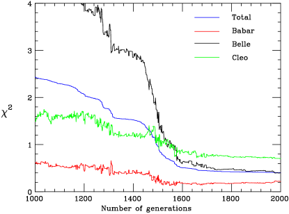
Dependence of the error function $E_{2}^{(0)}$ for a training of all three experiments on central experimental data. Note that at the end of the minimization $E_{2}^{(0)}\ll 1$ for all experiments.

The lepton energy spectrum, Eq. 6.32, as parametrized with a neural network, has to satisfy three constraints independently of the dynamics of the process. First of all, it is zero outside the region where it has kinematical support, in particular it has to vanish at the kinematical endpoints, $E_{l}=0$ and $E_{l}=E_{\max}$. Second, the spectrum is a positive definite quantity (since any integral over it is an observable, a partial branching ratio), therefore it must satisfy a local positivity condition.

As we have discussed in Section 5.2.4, there are several methods in our strategy to introduce kinematical constraints in an unbiased way. We have found that for the present application, the optimal method to implement the kinematical constraints that the spectrum should vanish at the endpoints is hard-wiring them into the parametrization, that is, the lepton energy spectrum parametrized by a neural net will be given by

$$\left(\frac{d\Gamma}{dE_{l}}\right)^{(\mathrm{net})(k)}(E_{l})=E_{l}^{n_{1}}\xi_{1}^{(L)}(E_{l})(E_{\max}-E_{l})^{n_{2}}\ ,$$ (6.33)

with $n_{1},n_{2}$ positive numbers, and $\xi_{1}^{(L)}$ is the output of the neural network for a given value of $E_{l}$. Assuming this functional behavior at the endpoints of the spectrum introduces no bias since it can be shown that our results do not depend on the value of $n_{1}$ and $n_{2}$. For the reference training we have verified that $n_{1}=1$ and $n_{2}=1$ are suitable values for these polynomial exponents.

We will impose the remaining kinematical constraint, the positivity constraint, as a Lagrange multiplier in the total error. That is, the total quantity to be minimized is the sum of two terms,

$$E_{\mathrm{tot}}^{(k)}=E_{2}^{(k)}+\lambda_{p}P\left[\left(\frac{d\Gamma}{dE_{l}}\right)^{(\mathrm{net})}\right]\ ,$$ (6.34)

where $E_{2}^{(k)}$ is Eq. 5.33 and the the positivity condition is implemented penalizing those configurations in which a region of the spectrum is negative,

$$P\left[\left(\frac{d\Gamma}{dE_{l}}\right)^{(\mathrm{net})}\right]=-\int_{0}^{E_{\max}}dE_{l}\left(\frac{d\Gamma}{dE_{l}}\right)^{(\mathrm{net})}(E_{l})\theta\left(-\left(\frac{d\Gamma}{dE_{l}}\right)^{(\mathrm{net})}(E_{l})\right),$$ (6.35)

since P is zero for a positive spectrum. The relative weight $\lambda_{p}$ is determined via a stability analysis, requiring that $\lambda_{p}$ is large enough so that the constraint is verified, but small enough so that experimental data can still be learned in an efficient way. As we will show in brief, the implementation of the kinematical constraints plays an essential role in the parametrization of the lepton spectrum. In particular, if kinematic constraints are not included in the fit the error at small $E_{l}$ grows very large and the extrapolation to $E_{0}=0$ becomes completely unreliable.

Figure 6.15:

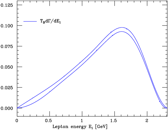
Lepton energy spectrum, Eq. 4.48, as parametrized by the Monte Carlo ensemble of neural networks. The bands represent the 1-$\sigma$ uncertainty region.

Figure 6.16:

Comparison of the different experimental moments, Eqns. 6.25-6.27 as obtained from our parametrization with the original measurements, as a function of the lower cut on the lepton energy $E_{0}$.

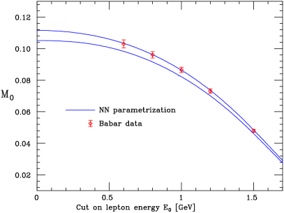
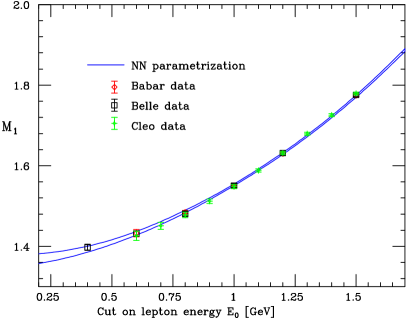
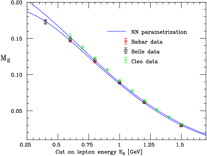
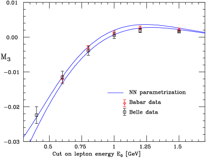
The set of neural networks parametrizing the lepton energy distribution trained on the Monte Carlo sample of replicas of the experimental data defines the probability measure in the space of lepton energy spectra. From this probability measure, as explained in Chapter 5, expectation values of functionals of the lepton spectrum can be computed as

$$\left\langle\mathcal{F}\left[\frac{d\Gamma}{dE_{l}}\right]\right\rangle\equiv\int\mathcal{D}\frac{d\Gamma}{dE_{l}}\mathcal{P}\left[\frac{d\Gamma}{dE_{l}}\right]\mathcal{F}\left[\frac{d\Gamma}{dE_{l}}\right]=\frac{1}{N_{\mathrm{rep}}}\sum_{k=1}^{N_{\mathrm{rep}}}\mathcal{F}\left[\left(\frac{d\Gamma}{dE_{l}}\right)^{(\mathrm{net})(k)}\right]\ .$$ (6.36)

We now present the results for this parametrization, from which averages and moments can be computed with the corresponding uncertainties. In Fig. 6.15 we plot the resulting lepton energy spectrum with uncertainties. In Fig. 6.16 we compare the computation of the moments of the lepton energy spectrum using our parametrization to the experimental results from Babar, Belle and Cleo. We observe good agreement for all the data points. As it has been explained in Section 5.3, it is crucial to validate the results of the parametrization using suitable statistical estimators. In Table 6.13 we have the most relevant statistical estimators for all the data points, and in Table 6.14 the same estimators for the different experiments included in the fit.

With the results described in this section the total branching ratio can be computed, even if experimental information was restricted to a finite value of $E_{0}$. This is possible because the continuity condition implicit in the neural network definition together with the kinematic constraints allow for an accurate extrapolation from the experimental data with lowest $E_{l}=0.4$ GeV to the kinematic endpoint $E_{l}=0$. Note that this is not true if the Belle data is not included in the fit, see Fig. 6.21. The result that is obtained for the partial decay rate, computed from the neural network sample,

$$\left\langle\mathcal{B}\left(B\to X_{c}l\nu\right)\right\rangle=\left\langle M_{0}(E_{l}=0)\right\rangle=\tau_{B}\frac{1}{N_{\mathrm{rep}}}\sum_{k=1}^{N_{\mathrm{rep}}}\int_{0}^{E_{\max}}dE_{l}\left(\frac{d\Gamma}{dE_{l}}\right)^{(\mathrm{net})(k)}\left(E_{l}\right)\ ,$$ (6.37)

is the total branching ratio,

$$\mathcal{B}\left(B\to X_{c}l\nu\right)=\left(10.8\pm 0.4\right)~{}10^{-2}\ ,$$ (6.38)

which is to be compared with the PDG result [pdg],

$$\mathcal{B}\left(B\to X_{c}l\nu\right)_{\mathrm{PDG}}=\left(10.2\pm 0.9\right)~{}10^{-2}\ ,$$ (6.39)

and with the direct Delphi measurement of the total branching ratio [delphifit], which is measured without restrictions on the lepton energy, which yields

$$\mathcal{B}\left(B\to X_{c}l\nu\right)_{\mathrm{Delphi}}=\left(10.5\pm 0.2\right)~{}10^{-2}\ .$$ (6.40)

Is is observed that the three results are compatible, even if our determination is somewhat closer, both in the central value and in the size of the uncertainty, to the Delphi measurement. The small error in our determination of $\mathcal{B}\left(B\to X_{c}l\nu\right)$ shows that the technique discussed in this work can be used also to extrapolate in a faithful way into regions where there is no experimental data available.

	10	100	1000
$\chi^{2}_{\mathrm{tot}}$	1.31	1.11	1.11
$\left\langle\chi^{2}\right\rangle$	2.50	2.23	2.21
$\left\langle PE\left[\left\langle M\right\rangle_{\mathrm{rep}}\right]\right\rangle$	9%	8%	5%
$r\left[M\right]$	0.999	0.999	0.999
$\left\langle PE\left[\sigma^{(\mathrm{net})}\right]\right\rangle_{\mathrm{dat}}$	67%	58%	10%
$\left\langle\sigma^{(\exp)}\right\rangle_{\mathrm{dat}}$	0.00267	0.00267	0.00267
$\left\langle\sigma^{(\mathrm{net})}\right\rangle_{\mathrm{dat}}$	0.00180	0.00168	0.00168
$r\left[\sigma^{(\mathrm{net})}\right]$	0.77	0.85	0.85
$\left\langle\rho^{(\exp)}\right\rangle_{\mathrm{dat}}$	0.166	0.166	0.166
$\left\langle\rho^{(\mathrm{net})}\right\rangle_{\mathrm{dat}}$	0.32	0.245	0.245
$r\left[\rho^{(\mathrm{net})}\right]$	0.35	0.38	0.38
$\left\langle\mathrm{cov}^{(\exp)}\right\rangle_{\mathrm{dat}}$	$1.4~{}10^{-6}$	$1.4~{}10^{-6}$	$1.4~{}10^{-6}$
$\left\langle\mathrm{cov}^{(\mathrm{net})}\right\rangle_{\mathrm{dat}}$	$7.8~{}10^{-7}$	$6.7~{}10^{-7}$	$6.7~{}10^{-7}$
$r\left[\mathrm{cov}^{(\mathrm{net})}\right]$	0.49	0.53	0.53

Table 6.13: Statistical estimators for the ensemble of trained neural networks, for 10, 100 and 1000 trained replicas.

	Babar	Belle	Cleo
$\chi^{2}_{\mathrm{tot}}$	0.42	1.81	1.14
$\left\langle\chi^{2}\right\rangle$	1.75	2.75	2.21
$\left\langle PE\left[\left\langle M\right\rangle_{\mathrm{rep}}\right]\right\rangle$	0.78%	18%	0.6%
$r\left[M\right]$	0.999	0.999	0.999
$\left\langle PE\left[\sigma^{(\mathrm{net})}\right]\right\rangle_{\mathrm{dat}}$	47%	60%	71%
$\left\langle\sigma^{(\exp)}\right\rangle_{\mathrm{dat}}$	0.0023	0.0021	0.0041
$\left\langle\sigma^{(\mathrm{net})}\right\rangle_{\mathrm{dat}}$	0.0016	0.0015	0.0020
$r\left[\sigma^{(\mathrm{net})}\right]$	0.91	0.89	0.96
$\left\langle\rho^{(\exp)}\right\rangle_{\mathrm{dat}}$	0.16	0.40	0.31
$\left\langle\rho^{(\mathrm{net})}\right\rangle_{\mathrm{dat}}$	0.17	0.21	0.33
$r\left[\rho^{(\mathrm{net})}\right]$	0.87	0.19	0.34
$\left\langle\mathrm{cov}^{(\exp)}\right\rangle_{\mathrm{dat}}$	$6.9~{}10^{-6}$	$1.5~{}10^{-6}$	$6.5~{}10^{-7}$
$\left\langle\mathrm{cov}^{(\mathrm{net})}\right\rangle_{\mathrm{dat}}$	$1.9~{}10^{-5}$	$1.4~{}10^{-6}$	$2.6~{}10^{-7}$
$r\left[\mathrm{cov}^{(\mathrm{net})}\right]$	0.98	0.47	-0.04

Table 6.14: Statistical estimators for the ensemble of trained neural networks, for those experiments included in the fit. The replica sample consists of $N_{\mathrm{rep}}=$1000 neural networks.

Figure 6.17:

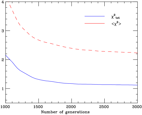
Total $\chi^{2}_{\mathrm{tot}}$, Eq. 5.76, of the replica sample, compared with average error, $\left\langle\chi^{2}\right\rangle$.

Figure 6.18:

Average error of the data points as computed from the neural network sample, Eq. 5.17, as compared with the experimental value (left). Dependence during the training of the values of the scatter correlations, Eq. 5.90, during the training, for the Babar experimental data (right).

Figure 6.19:

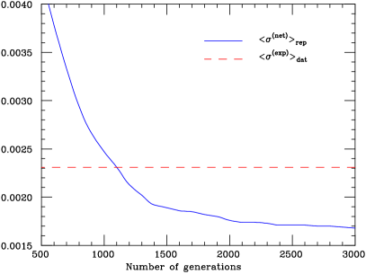
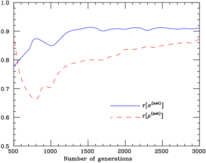
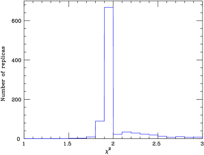
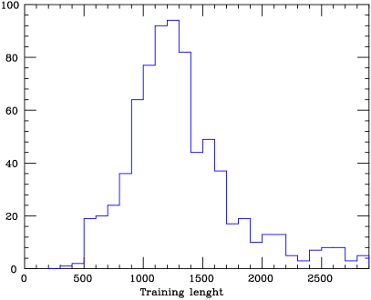
Distribution of error functions, $E_{2}^{(k)}$, over the sample of trained replicas (left) and distribution of training lenghts in GA generations (right).

Figure 6.20:

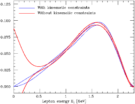
Comparison of the lepton energy spectrum when no kinematic constraints are incorporated.

Figure 6.21:

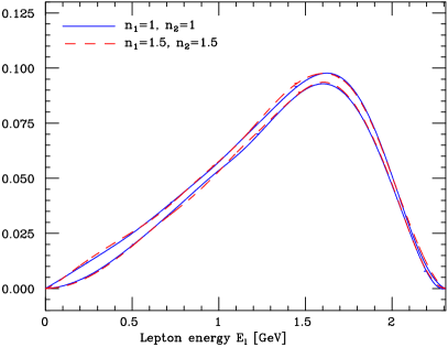
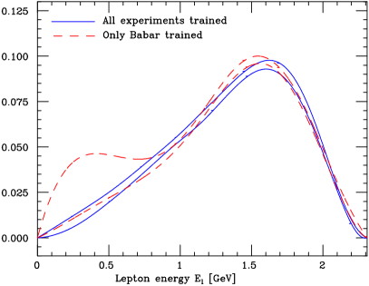
Comparison of the lepton energy spectrum when the parameters $n_{1}$ and $n_{2}$ are changed (left). Comparison of the lepton energy spectrum when only Babar data is incorporated in the fit with the result when all experiments are incorporated in the fit (right).

Important information on the quality of the fit can be obtained from the analysis of the dependence of the different statistical estimators with respect to the number of genetic algorithms generations, like the total $\chi^{2}$ or the average error. This dependence is represented in Fig. 6.17. Note that at the end of the training $\chi^{2}_{\mathrm{tot}}\sim 1$ and $\left\langle\chi^{2}\right\rangle\sim 2$, as expected. Note also that the fit has reached convergence since the $\chi^{2}_{\mathrm{tot}}$ profile is very flat for a large number of generations.

This can be repeated for other statistical estimators, like for example the average spread of the data points as computed from the neural network ensemble, defined in Section 5.3.1, which is compared with the same quantity computed from the experimental data, $\sigma_{i}^{(\mathrm{exp})}$ in Fig. 6.18 as a function of the number of genetic algorithms generations. The fact that one has error reduction, as has been explained in [f2ns], is the sign that the network has found an underlying law to the experimental data, in this case the lepton energy spectrum.

Another relevant estimator is the scatter correlations of the spread of the points (see Fig. 6.18). One can define similarly a scatter correlation for the net correlation $\rho_{ij}^{(\mathrm{net})}$, also represented in Fig. 6.18 for the Babar experimental data. We observe that when the training ends both values of $r$ are close to 1, a sign that errors and correlations are being faithfully reproduced. Another relevant estimator of the goodness of the fit is the distribution of both $E_{2}^{(k)}$ and of the training lengths over the replica sample, see Fig. 6.19. We have checked that these two distributions satisfy the requirements described in Section 5.3.

We can compare also fits with and without the inclusion of kinematical constraints, to see which is the effect of their implementation. The endpoint constraint at $E_{l}=E_{\max}$ is crucial to obtain convergent results. In Fig. 6.20 one can observe that when the endpoint constraint at $E_{l}=0$ and the positivity constraint are removed the error becomes very large at small $E_{l}$, and on top of that sightly negative at large $E_{l}$ near the endpoint. Note that the physical value for the spectrum at the endpoint, $d\Gamma/dE_{l}(E_{l}=0)=0$, is contained within the small-$E_{l}$ error bars, as expected.

In Fig. 6.21 we show a comparison of a fit of a single experiment, Babar. We observe that when only the Babar data is incorporated in the fit, the error at small values of $E_{l}$ is much larger. This is so because, as discussed above, the Belle data, which extends to lower values of $E_{l}$, is crucial to determine the low $E_{l}$ behavior of the lepton spectrum. Finally, in Fig. 6.21 we show that our results are independent of the precise choice of $n_{1}$ and $n_{2}$ in Eq. 6.33. In particular using $n_{1}=1.5$ and $n_{2}=1.5$ results in the same fit as when using the reference values, $n_{1}=1$ and $n_{2}=2$.

As one example of the applications of the present parametrization of the lepton energy spectrum, in this section our results are compared with the theoretical calculation of Ref. [agru] (AGRU). Their formalism allows the computation of moments of arbitrary differential distributions from semileptonic B meson decays, with arbitrary kinematical cuts, like the lepton energy spectrum in charmed decays that is analyzed in the present work. In particular their computation of the lepton energy spectrum will be studied, which they define as

$$N_{k}\equiv\frac{1}{\Gamma_{\mathrm{LO}}}\int_{E_{0}}^{E_{\max}}dE_{l}dq^{2}dr\tilde{E}_{l}^{k}\frac{d^{3}\Gamma}{dE_{l}drdq^{2}}\ ,$$ (6.41)

with $\tilde{E}\equiv E/m_{b}$, and where the leading order partonic semileptonic decay rate $\Gamma_{\mathrm{LO}}$ is given by

$$\Gamma_{\mathrm{LO}}=\Gamma_{0}|V_{cb}|^{2}z_{0}(\rho)\ ,$$ (6.42)

where $\Gamma_{0}$ is defined in Eq. 4.51, $\rho\equiv m_{c}^{2}/m_{b}^{2}$ and the phase space factor is defined in Eq. 4.41. These moments can be related to the experimentally measured moments, defined in Eqns. 6.25- 6.27, in a straightforward way, for example for the first two moments one has

$$M_{0}=\tau_{B}\Gamma_{0}N_{0},\qquad M_{1}=m_{b}\frac{N_{1}}{N_{0}}\ ,$$ (6.43)

and similarly for the other moments.

Figure 6.22:

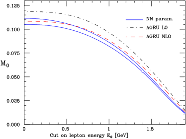
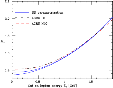
Comparison of the results of Ref. [agru] on the partial branching ratio Eq. 6.25 both at leading order (LO) and at next-to-leading order (NLO) with the same quantity computed from our parametrization.

Figure 6.23:

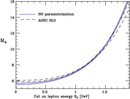
Comparison of the results of Ref. [agru] on the $n=4$ moment and at next-to-leading order (NLO), with the corresponding theoretical uncertainties, with the same quantity computed from the neural network parametrization parametrization.

In Figs. 6.22 the results of [agru] both at leading order (LO) and at next-to-leading order (NLO) are compared with the moments obtained from our parametrization as a function of the lower cut in the lepton energy $E_{0}$. Comparing results at different perturbative orders is interesting to asses the behavior of the perturbative expansion. One should take into account in this comparison that the results of [agru] are purely perturbative, therefore the difference between the two results could be an indicator of the size of the missing nonperturbative corrections. Another interesting feature is that while for $M_{0}$, the partial branching fraction, the NLO corrections are sizable and bring the theoretical prediction in better agreement with the experimental measurement, for $M_{1}$ (which is the ratio of two perturbative expansions) the size of the perturbative corrections is much smaller. In addition, we show in Fig. 6.23 the comparison for the $n=4$ moment (not measured experimentally) with an estimation of the uncertainties in the theoretical prediction, as described in [bmeson].

A more general comparison with theoretical predictions should include also the known nonperturbative power corrections up to order $\mathcal{O}(1/m_{b}^{3})$ to the expressions for the moments of the spectrum, since in this case the difference of the theoretical results from our parametrization would indicate the size of the missing unknown corrections, both perturbative and nonperturbative. A more detailed study of this point, together with an analysis of possible violations of local quark-hadron duality [shifman], is left for future work.

As another application of our parametrization of the lepton energy spectrum, it will be used to determine the b quark mass $m_{b}^{1S}$ from the experimental data using a novel strategy. To this purpose the technique of Ref. [bauertrott] will be used, which consists on the minimization of the size of higher order corrections to obtain sets of moments of the lepton energy spectrum which have reduced theoretical uncertainty for the extraction of nonperturbative parameters like $\bar{\Lambda}_{1S}$ and $\lambda_{1}$. In Ref. [bmeson] we describe in detail the method we use to determine the b quark mass from our neural network parametrization of the leptonic spectrum, which is summarized here.

The moments that minimize the impact of the higher order nonperturbative corrections are given by

$$R_{1}\equiv\frac{\int_{1.3}^{E_{\max}}E_{l}^{1.4}\frac{d\Gamma}{dE_{l}}dE_{l}}{\int_{1}^{E_{\max}}E_{l}\frac{d\Gamma}{dE_{l}}dE_{l}}\ ,$$ (6.44)

and

$$R_{2}\equiv\frac{\int_{1.4}^{E_{\max}}E_{l}^{1.7}\frac{d\Gamma}{dE_{l}}dE_{l}}{\int_{0.8}^{E_{\max}}E_{l}^{1.2}\frac{d\Gamma}{dE_{l}}dE_{l}}\ .$$ (6.45)

The full expression for this moments in terms of heavy-quark non-perturbative parameters can be found in Ref. [bauertrott]. These leptonic moments $R_{1}$ and $R_{2}$ depend on 9 nonperturbative parameters, up to $\mathcal{O}(1/m_{b}^{3})$: $\bar{\Lambda}_{1S}$, $\lambda_{1}$ and $\lambda_{2}$, and six matrix elements, $\rho_{1},\rho_{2},\tau_{1},\tau_{2},\tau_{3}$ and $\tau_{4}$, that contribute at order $1/m_{b}^{3}$ in the heavy quark expansion, of which not all of them are independent [gremm, shapevar].

The most relevant feature of these leptonic moments $R_{1}$ and $R_{2}$ is that they have non-integer powers and to the best of our knowledge have not been yet experimentally measured, at least in a published form. Therefore, the values of $R_{1}$ and $R_{2}$ that will be used in this analysis are extracted from our neural network parametrization of the lepton spectrum, which allows the computation of arbitrary moments, together with their associated error and correlation. Let us recall that the central values are determined as

$$\left\langle R_{1}^{(\mathrm{net})}\right\rangle=\frac{1}{N_{\mathrm{rep}}}\sum_{k=1}^{N_{\mathrm{rep}}}R_{1}^{(\mathrm{net})(k)},\qquad R_{1}^{(\mathrm{net})(k)}=\frac{\int_{1.3}^{E_{\max}}E_{l}^{1.4}\frac{d\Gamma^{(\mathrm{net})(k)}}{dE_{l}}(E_{l})dE_{l}}{\int_{1}^{E_{\max}}E_{l}\frac{d\Gamma^{(\mathrm{net})(k)}}{dE_{l}}(E_{l})dE_{l}}\ ,$$ (6.46)

and similarly for $R_{2}$, and the error and the correlation of the moments $R_{1}$ and $R_{2}$ are computed in the standard way. The following values for the moments with the associated errors and their correlation are obtained,

$$R_{1}^{(\mathrm{net})}=1.017\pm 0.003,\quad R_{2}^{(\mathrm{net})}=0.938\pm 0.004,\quad\rho_{12}=0.94\ ,$$ (6.47)

that as expected are highly correlated. Then to determine the nonperturbative parameters $\Lambda_{1S}$ and $\lambda_{1}$ the associated $\chi^{2}_{\mathrm{fit}}$ is minimized,

$$\chi^{2}_{\mathrm{fit}}=\sum_{i,j=1}^{2}\left(R_{i}^{(\mathrm{net})}-R_{i}^{(\mathrm{th})}\right)\left(\mathrm{cov}^{-1}\right)_{ij}\left(R_{j}^{(\mathrm{net})}-R_{j}^{(\mathrm{th})}\right)\ ,$$ (6.48)

where $\mathrm{cov}^{-1}_{ij}$ is the inverse of the covariance matrix associated to the two moments $R_{1}^{(\mathrm{net})}$ and $R_{2}^{(\mathrm{net})}$, and $R_{i}^{(\mathrm{th})}\left(\bar{\Lambda}_{1S},\lambda_{1}\right)$ is the theoretical prediction for these moments as a function of the two nonperturbative parameters [bauertrott].

Once the values of $\bar{\Lambda}_{1S}$ and $\lambda_{1}$ have been determined from the minimization of Eq. 6.48, one obtains for the b quark mass $m_{b}^{1S}$ mass in the 1S scheme the following value:

$$m_{b}^{1S}=\bar{m}_{B}-\bar{\Lambda}_{1S}=\left(4.84\pm 0.16^{\mathrm{exp}}\pm 0.05^{\mathrm{th}}\right)~{}\mathrm{GeV}=\left(4.84\pm 0.17^{\mathrm{tot}}\right)~{}\mathrm{GeV}\ ,$$ (6.49)

From the above results one observes that the dominant source of uncertainty is the experimental uncertainty, that is, the uncertainty associated to our parametrization of the lepton energy spectrum. This determination of the b quark mass is consistent with determinations from other analysis. The b quark mass has been determined using different techniques, like the sum rule approach, using either non-relativistic [hoang, benekesum, pinedasumrule] or relativistic [kuhnbmass, corcella] sum rules, global fits of moments of differential distributions in B decays, [bauerglobalfit, delphifit, fitskin], the renormalon analysis of Ref. [pineda], and several other methods related to heavy-quarkonium physics [quarkonium1, quarkonium2] (see [quarkonium3] for a review). To compare our results with some of the above references, it is useful to relate the $m^{1S}_{b}$ mass to the MS-bar $\bar{m}_{b}\left(\bar{m}_{b}\right)$ mass [hoangfull], and once the conversion is performed the value

$$\bar{m}_{b}\left(\bar{m}_{b}\right)=\left(4.31\pm 0.17^{\mathrm{tot}}\right)~{}\mathrm{GeV}\ ,$$ (6.50)

is obtained, where we have used $\alpha_{s}(M_{Z}^{2})=0.1182$ and included perturbative corrections up to two loops. It turns out that our determination of $m^{1S}_{b}$ is not competitive with respect to other determinations due to the large uncertainties associated to the fact that only two moments we use in the determination of these parameters. The inclusion of additional moments in the fit would constrain more the nonperturbative parameters and reduce the experimental uncertainty associated to them.

For the nonperturbative parameter $\lambda_{1}$ the following value is obtained

$$\lambda_{1}=\left(-0.17\pm 0.15^{\mathrm{exp}}\pm 0.05^{\mathrm{th}}\right)~{}\mathrm{GeV^{2}}=\left(-0.17\pm 0.16^{\mathrm{tot}}\right)~{}\mathrm{GeV^{2}}\ .$$ (6.51)

As in the determination of $\bar{\Lambda}_{1S}$ it can be seen that the theoretical uncertainties are smaller than the experimental ones, which are the dominant ones. Our result for the parameter $\lambda_{1}$ is consistent with other extractions in the context of global fits of B decay data [bauerglobalfit, delphifit], but again not competitive due to the rather large uncertainties.

To summarize, in this part of the thesis we have presented a determination of the probability density in the space of the lepton energy spectrum from semileptonic B meson decays, based on the latest available data from the Babar, Belle and Cleo collaborations. In addition, this application shows the implementation of a well defined strategy to reconstruct functions with uncertainties when the only available experimental information comes through convolutions of these functions. As a byproduct of our analysis, using our parametrization of the lepton spectrum, we have extracted the nonperturbative parameters $\bar{\Lambda}_{1S}$ and $\lambda_{1}$, with a method that reduces the contributions from the theoretical uncertainties.

The number of possible applications of this strategy to other problems in B physics is rather large, and is discussed in some detail in Ref. [bmeson]. The most promising application is to use our neural network strategy to construct a parametrization of the shape function $S(k)$ of the B meson, a universal characteristic of the B meson governing inclusive decay spectra in processes with massless partons in the final state, as extracted from the $B\to X_{s}\gamma$ and $B\to X_{u}l\nu$ decay modes. In this case we have additional theoretical information on its behaviour. For example, at tree level its moments

$$A_{n}\equiv\int dkk^{n}S(k)\ ,$$ (6.52)

have to satisfy $A_{0}=1,A_{1}=0$ and $A_{2}=\mu_{\pi}^{2}/3$, where $\mu_{\pi}$ is a nonperturbative parameter of the heavy quark expansion. At higher orders these relations are theoretically more controversial [neubertfactorization, shapemanohar]. Since the uncertainty from the extraction of $S(k)$ is the dominant source of theoretical uncertainty in some CKM matrix elements extractions, it would therefore be interesting to estimate again this uncertainty using the technique presented in this work, since in the current approach [shape2] the shape function uncertainties are estimated in a rather crude way, just trying different functional forms compatible with the theoretical constraints.

6.4 Parton distribution functions

In this Section we describe the most important application of the general strategy introduced in Chapter 5. Indeed, it was the determination of the probability measure in the space of parton distributions the main motivation for the development of the technique that is the main subject of this thesis. First we describe an alternative approach to evolve parton distributions, required by the use of neural networks as interpolants for parton distributions, and then we present results on the neural network parametrization of the nonsinglet parton distribution $q_{NS}(x,Q_{0}^{2})$ from experimental data on the nonsinglet structure function $F_{2}^{NS}(x,Q^{2})$.

6.4.1 A new approach to parton evolution

In order to construct the probability measure in the space of nonsinglet parton distributions, for reasons to be described in the following, we need a dedicated parton evolution formalism. In this Section the strategy that will be used for the evolution of parton distributions is introduced. For the present application only nonsinglet parton distributions will be considered, and therefore the description of this parton evolution technique will be restricted to the nonsinglet sector. This discussion can be generalized straightforwardly to the singlet sector and will be throughly described in Ref. [nnsinglet].

There are two classes of methods for solving the perturbative QCD DGLAP evolution equations, introduced in Section 4.1.2: the N-space methods (like the one described in [pegasus]) which solve analytically the DGLAP evolution equations in Mellin space and then compute the inverse Mellin transformation to x-space, and the x-space methods (like [qcdnum]), which perform a direct numerical integration of the integro-differential DGLAP equations. Both methods have different advantages and drawbacks, but in principle they lead to a similar accuracy in the evolution of parton distributions, as shown in the dedicated analysis of Ref. [lh]. However, since we are going to parametrize parton distributions not with simple functional forms but with neural networks, none of the standard techniques can be applied to our case. For example, in standard N-space evolution codes one needs to perform the Mellin transform of the parton distribution and extend it to complex values of N, but in our case this is not allowed since an analytical expansion of neural networks to complex values of the inputs and the outputs is mathematically ill-defined.

Hence we need to use a hybrid strategy: we will solve the DGLAP evolution equations [gl, ap, dok] in N-space, introduced in Section 4.1.2, and then we will Mellin invert only the evolution factor $\Gamma(N)$ in Eq. 4.35, so that the evolved x-space parton distribution $q(x,Q^{2})$ can be written as the convolution of the x-space parton distribution at the initial evolution scale $q(x,Q^{2}_{0})$ and an x-space evolution factor $\Gamma(x)$. Schematically, we will have

$$q(x,Q^{2})=\Gamma(x)\otimes q(x,Q_{0}^{2}),\qquad\Gamma(N)\equiv\int_{0}^{1}dxx^{N-1}\Gamma(x)\ .$$ (6.53)

Then we will interpolate the x-space evolution factor $\Gamma(x)$, so that the heavy numerical task of its computation is decoupled from the determination of the parameters describing the parton distribution from experimental data. With all these considerations taken into account one ends up with a fast and efficient evolution code, which will described in this Section.

First of all we define the notation that will be used for the strong coupling constant. The convention that we use is

$$Q^{2}\frac{da_{s}(Q^{2})}{Q^{2}}=-\sum_{k=0}^{\infty}\beta_{k}a_{s}(Q^{2})^{k+1},\qquad a_{s}(Q^{2})=\frac{\alpha_{s}(Q^{2})}{4\pi}\ ,$$ (6.54)

where the beta function coefficients are given by

$$\beta_{0}=11-\frac{2N_{f}}{3},\qquad\beta_{1}=102-\frac{38}{3}N_{f}\ ,$$ (6.55)

the scheme-dependent coefficent $\beta_{2}$ is given in [pegasus], and $N_{f}$ is the number of active quark flavors.

The explicit solution for the above equation at the NNLO accuracy can be written in terms of a boundary condition $\alpha_{s}\left(M_{Z}^{2}\right)$ and is given by

$$\alpha_{s}\left(Q^{2}\right)_{\mathrm{NNLO}}=\alpha_{s}\left(Q^{2}\right)_{\mathrm{LO}}\left(1+\alpha_{s}\left(Q^{2}\right)_{\mathrm{LO}}\left(\alpha_{s}\left(Q^{2}\right)_{\mathrm{LO}}-\alpha_{s}\left(M_{Z}^{2}\right)\right)(b_{2}-b_{1}^{2})+\alpha_{s}\left(Q^{2}\right)_{\mathrm{NLO}}b_{1}\ln\frac{\alpha_{s}\left(Q^{2}\right)_{\mathrm{NLO}}}{\alpha_{s}\left(M_{Z}^{2}\right)}\right)\ ,$$ (6.56)

where we have defined in a recursive way,

$$\alpha_{s}\left(Q^{2}\right)_{\mathrm{NLO}}=\alpha_{s}\left(Q^{2}\right)_{\mathrm{LO}}\left(1-b_{1}\alpha_{s}\left(Q^{2}\right)_{\mathrm{LO}}\ln\left(1+\beta_{0}\alpha_{s}\left(M_{Z}^{2}\right)\ln\frac{Q^{2}}{M_{Z}^{2}}\right)\right)\ ,$$ (6.57)

$$\alpha_{s}\left(Q^{2}\right)_{\mathrm{LO}}=\frac{\alpha_{s}\left(M_{Z}^{2}\right)}{1+\beta_{0}\alpha_{s}\left(M_{Z}^{2}\right)\ln\frac{Q^{2}}{M_{Z}^{2}}}\ .$$ (6.58)

and we have defined $b_{k}=\beta_{k}/\beta_{0}$.

The evolution equations for nonsinglet combinations of parton distributions, as we have seen in Section 4.1.2, read in Mellin space

$$\frac{d}{d\ln Q^{2}}q^{i}_{NS}(N,Q^{2})=\frac{\alpha_{s}\left(Q^{2}\right)}{2\pi}\gamma_{NS}^{i}(N,\alpha_{s}\left(Q^{2}\right))q_{NS}^{i}(N,Q^{2})\ ,$$ (6.59)

where $i=\pm,v$ stand for the three different nonsinglet combinations that evolve independently at NNLO, given by

$$q_{NS,ik}^{\pm}=q_{i}\pm\bar{q}_{i}-\left(q_{k}\pm\bar{q}_{k}\right),\qquad q_{NS}^{v}=\sum_{r=1}^{N_{f}}\left(q_{r}-\bar{q}_{r}\right)\ .$$ (6.60)

In the following discussion we assume that in each case we use the appropriate anomalous dimension for each type of nonsinglet parton distribution, and since we are restricted now to the analysis of nonsinglet parton distributions, we will assume also that all quantities (parton distributions or anomalous dimensions) correspond to this nonsinglet sector. The nonsinglet anomalous dimension has been computed in powers of $\alpha_{s}\left(Q^{2}\right)$ up to NNLO,

$$\gamma\left(N,\alpha_{s}\left(Q^{2}\right)\right)=\gamma^{(0)}(N)+\frac{\alpha_{s}\left(Q^{2}\right)}{4\pi}\gamma^{(1)}(N)+\left(\frac{\alpha_{s}\left(Q^{2}\right)}{4\pi}\right)^{2}\gamma^{(2)}(N)\ ,$$ (6.61)

where the N-space anomalous dimension was computed at LO in Ref. [ap], at NLO in Ref. [petronzio], and recently the full NNLO contribution was computed in Ref. [mvvns]. The leading order nonsinglet anomalous dimension has the explicit form

$$\gamma^{(0)}(N)=C_{F}\left[3-4\sum_{k=1}^{N}\frac{1}{k}+\frac{2}{N(N+1)}\right]\ ,\qquad C_{F}=\frac{4}{3}\ ,$$ (6.62)

which has the following large-N limit,

$$\lim_{N\to\infty}\gamma^{(0)}(N)=-4C_{F}\ln N\ +\mathcal{O}\left(N^{0}\right),$$ (6.63)

which will be needed for the computation of the large-x limit of the x-space evolution factor $\Gamma(x)$.

The solution to the nonsinglet evolution equation, Eq. 6.59, reads at NNLO accuracy

$$q(N,Q^{2})=\Gamma(N,\alpha_{s}\left(Q^{2}\right),\alpha_{s}\left(Q^{2}_{0}\right))q(N,Q^{2}_{0})\ ,$$ (6.64)

where the N-space evolution factor $\Gamma(N)$ is given by

$$\Gamma(N,\alpha_{s}\left(Q^{2}\right),\alpha_{s}\left(Q^{2}_{0}\right))=\left(\frac{\alpha_{s}\left(Q^{2}\right)}{\alpha_{s}\left(Q^{2}_{0}\right)}\right)^{-\gamma^{(0)}(N)/\beta_{0}}\Bigg{(}1-\left(\alpha_{s}\left(Q^{2}\right)-\alpha_{s}\left(Q^{2}_{0}\right)\right)U_{NS}^{(1)}(N)$$

$$+\left(\alpha_{s}\left(Q^{2}\right)^{2}-\alpha_{s}\left(Q^{2}_{0}\right)^{2}\right)U_{NS}^{(2)}(N)-\alpha_{s}\left(Q^{2}\right)\alpha_{s}\left(Q^{2}_{0}\right)\left(U_{NS}^{(1)}(N)\right)^{2}\Bigg{)}\ ,$$ (6.65)

where we have defined the nonsinglet evolution coefficients as

$$U_{NS}^{(1)}(N)=-\frac{1}{\beta_{0}}\left(\gamma^{(1)}(N)-b_{1}\gamma^{(0)}(N)\right)\ ,$$ (6.66)

$$U_{NS}^{(2)}(N)=-\frac{1}{2}\left(\frac{1}{\beta_{0}}\gamma^{(2)}(N)+b_{1}U_{NS}^{(1)}(N)-\frac{b_{2}}{\beta_{0}}\gamma^{(0)}(N)\right)\ .$$ (6.67)

Once we have solved the DGLAP equations in Mellin space, Eq. 6.64, we Mellin invert the evolution factor in Eq. 6.4.1 to perform parton evolution in x-space. Using the convolution theorem one can check that the x-space evolved parton distribution is given by

$$q(x,Q^{2})=\int_{x}^{1}\frac{dy}{y}\Gamma(y,\alpha_{s}\left(Q^{2}\right),\alpha_{s}\left(Q^{2}_{0}\right))q\left(\frac{x}{y},Q_{0}^{2}\right)\ ,$$ (6.68)

where the evolution kernel $\Gamma(x)$ is the Mellin inverse of Eq. 6.4.1,

$$\Gamma(x,\alpha_{s}\left(Q^{2}\right),\alpha_{s}\left(Q^{2}_{0}\right))=\int_{c-i\infty}^{c+i\infty}\frac{dN}{2\pi i}x^{-N}\Gamma(N,\alpha_{s}\left(Q^{2}\right),\alpha_{s}\left(Q^{2}_{0}\right))\ ,$$ (6.69)

where $c$ lies to the right of the rightmost singularity of $\Gamma(N)$. That is, one can check that the Mellin transform of the LHS of Eq. 6.68 is equal to the RHS of Eq. 6.64,

$$\int_{0}^{1}dxx^{N-1}q(x,Q^{2})=\Gamma\left(N,\alpha_{s}\left(Q^{2}\right),\alpha_{s}\left(Q^{2}_{0}\right)\right)q(N,Q_{0}^{2})\ .$$ (6.70)

The complicated numerical task in this evolution formalism is the numerical computation of the Mellin inverse transformation, Eq. 6.69. However note that as opposite to standard N-space parton evolution methods, the evolution of the parton distribution can be decoupled from the Mellin inversion of the evolution factor, which is the most time consuming task.

We will use the Fixed Talbot algorithm to perform the numerical inversion of the Mellin transform Eq. 6.69. For a detailed description of this algorithm and its efficiency see Refs. [ft, ft2]. The Fixed Talbot algorithm for the numerical inversion of Mellin-Laplace transforms is specially accurate for the following reason: the numerical computation of inverse Mellin transforms is in general difficult since the integrand is highly oscillatory since the integration path moves through the complex plane. The Fixed Talbot algorithm bypasses this problem by choosing a path in the complex plane which minimizes the imaginary part of the integrand and therefore minimizes the impact of these oscillations. In the Fixed Talbot algorithm a generic inverse Mellin transform is computed as

$$f(x)=\frac{1}{2\pi i}\int_{C}x^{-N}f(N)dN\ ,$$ (6.71)

where the Talbot path $C$ is defined by the condition

$$N(\theta)=r\theta\left(1/\tan\theta+i\right),\quad-\pi\leq\theta\leq\pi\ ,$$ (6.72)

$$r\equiv\frac{2M}{5\ln\frac{1}{x}}\ ,$$ (6.73)

where M is the number of required precision digits. The Talbot path minimizes the contribution from oscillatory terms to the inverse Mellin Eq. 6.71, and therefore avoids the associated numerical instabilities. The resulting integral, Eq. 6.71, can be computed with adaptative gaussian quadratures to any desired accuracy.

The x-space evolution factor $\Gamma\left(x,\alpha_{s}\left(Q^{2}\right),\alpha_{s}\left(Q^{2}_{0}\right)\right)$, Eq. 6.69, has a flat behavior at intermediate $x$ together with a growing at both large and small $x$, where the behavior in both limits can be computed analytically. Now the explicit analytic expressions for the evolution factor $\Gamma(x)$ at both large $x$ and small $x$ will be computed. These results are interesting both for themselves, to obtain a more quantitative understanding of our evolution technique, and also for practical purposes, since they allow to perform a more efficient interpolation of $\Gamma(x)$. In Fig. 6.24 we represent the x-space evolution factor $\Gamma(x)$ for different perturbative orders and different evolution lenghts. Note that in the $x$ range relevant for nonsinglet evolution, $x\geq 5~{}10^{-3}$, the perturbative expansion for $\Gamma(x)$ appears to be near to convergence at the NNLO level. Note also that the small-x behaviour is very smooth in the relevant x range, unlike the large-x one.

Figure 6.24:

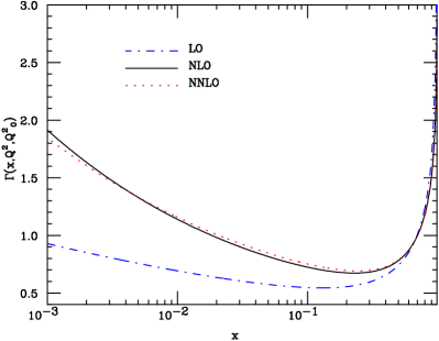
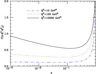
The x-space evolution factor $\Gamma\left(x,\alpha_{s}\left(Q^{2}\right),\alpha_{s}\left(Q^{2}_{0}\right)\right)$ for different perturbative orders at $Q^{2}=10^{4}$ GeV${}^{2}$ (left) and for different evolution lenghts at leading order (right). In all cases the starting evolution scale is $Q_{0}^{2}=2$ GeV${}^{2}$. Note the sharp rise of the evolution factor at large values of $x$.