CP3-06-01

Is $V_{tb}\simeq 1$?

J. Alwall, R. Frederix, J.-M. Gérard, A. Giammanco, M. Herquet,
S. Kalinin, E. Kou, V. Lemaître, F. Maltoni

Centre for Particle Physics and Phenomenology (CP3)

Université Catholique de Louvain

Chemin du Cyclotron 2

B-1348 Louvain-la-Neuve, Belgium

The strongest constraint on $V_{tb}$ presently comes from the $3\times 3$ unitarity of the CKM matrix, which fixes $V_{tb}$ to be very close to one. If the unitarity is relaxed, current information from top production at Tevatron still leaves open the possibility that $V_{tb}$ is sizably smaller than one. In minimal extensions of the standard model with extra heavy quarks, the unitarity constraints are much weaker and the EW precision parameters entail the strongest bounds on $V_{tb}$. We discuss the experimental perspectives of discovering and identifying such new physics models at the Tevatron and the LHC, through a precise measurement of $V_{tb}$ from the single top cross sections and by the study of processes where the extra heavy quarks are produced.

1 Introduction

The value of the CKM matrix element $V_{tb}$, related to the top-bottom charged current, is often considered to be known to a very satisfactory precision ($0.9990<\left|V_{tb}\right|<0.9992$ at 90% C.L. [1]). However, this range is determined using a full set of tree-level processes and relies on the unitarity of the $3\times 3$ CKM matrix. The unitary assumption is mainly supported by three experimental facts:

1. The measurement of $V_{ub}$ and $V_{cb}$ in $B$ mesons decays. We now know that the hierarchy of the elements belonging to the first two rows of the CKM matrix is in excellent agreement with the unitary condition. This is particularly evident within the Wolfenstein’s parametrization in terms of $\lambda\equiv\sin\theta_{c}\simeq 0.22$ where $\theta_{c}$ is the Cabibbo angle.

2. The recent DØ and CDF results on $\Delta M_{B_{s}}$ [2, 3]:

   $$17\ \mbox{ps}^{-1}<\Delta M_{B_{s}}<21\ \mbox{ps}^{-1}\quad{\mbox{(90\% C.L. interval)}}\quad$$ DØ collaboration (1)

   $$17.33^{+0.42}_{-0.21}{\rm(stat.)}\pm 0.07{\rm(syst.)}\ \mbox{ps}^{-1}\quad\ \quad \mbox{CDF collaboration }.$$ (2)

   The rather precise CDF measurement allows us to extract the ratio $|V_{td}/V_{ts}|$

   $$0.20<|V_{td}/V_{ts}|<0.22\,,$$ (3)

   by using $\Delta M_{B_{d}}/\Delta M_{B_{s}}$ (see, e.g., Ref. [1]) and taking into account the theoretical uncertainty associated with the hadronic matrix elements [4]. This ratio fits well with the unitary hypothesis which predicts it to be of order $\lambda$. One should emphasize however, that these processes come from loop diagrams, and could be polluted by new physics contributions.

3. The Tevatron measurements of $R$ based on the relative number of $t\bar{t}$-like events with zero, one and two tagged $b$-jets. The resulting values for $R$ are $1.12^{+0.27}_{-0.23}~{}\rm(stat.+syst.)$ [5] and $1.03^{+0.19}_{-0.17}~{}\rm(stat.+syst.)$ [6] for CDF and DØ respectively, both giving $R>0.61$ at 95% confidence level. Recalling the definition

   $$R\equiv\frac{\left|V_{tb}\right|^{2}}{\left|V_{td}\right|^{2}+\left|V_{ts}\right|^{2}+\left|V_{tb}\right|^{2}},$$ (4)

   it is clear that $R\simeq 1$ implies a strong hierarchy between $V_{tb}$ and the other two matrix elements, as expected in the unitary case. As we will argue later on, the upper limits of the single top production cross sections from Tevatron might already provide (rather loose) additional constraints on their absolute magnitude, $|V_{ts}|\raise 1.29167pt\hbox{$\;<$\kern-7.5pt\raise-4.73611pt\hbox{$\sim\;$}}0.62$ and $|V_{td}|\raise 1.29167pt\hbox{$\;<$\kern-7.5pt\raise-4.73611pt\hbox{$\sim\;$}}0.46$.

On the other hand, contrary to what has sometimes been argued, none of these experimental facts are directly constraining $V_{tb}$. In fact, even its “direct” determination from $R$, giving $\left|V_{tb}\right|>0.78$ at 95% C.L., comes simply from taking the square root of $R$, assuming the unitarity of the CKM matrix. Since no single top cross section measurement yet exists, the $V_{tb}\neq 1$ alternative should be considered as still acceptable. This possibility appears, for example, if one introduces new heavy up- and/or down-type quarks. Though such new fermions are not favoured by current precision constraints, they are not yet excluded, and their existence is in fact predicted by many extensions of the Standard Model (SM) [7]. We should thus keep in mind that the familiar $3\times 3$ CKM matrix might well be a submatrix of a $3\times 4$, $4\times 3$, $4\times 4$ or even larger matrix.

In the following section, we present two minimal extensions of the SM that allow a value for $V_{tb}$ considerably different from one. Although these models are theoretically self-consistent, they should be primarily regarded as motivations for further experimental scrutiny of $V_{tb}$. In the first case, the introduction of a new vector-like top singlet leads to a global rescaling of $V_{td}$, $V_{ts}$ and $V_{tb}$ leaving $R$ unchanged. In the second case, a complete new fourth generation is added and the $R$ measurement is used as a direct constraint. In Section 3, we discuss the expected precision on the extraction of $V_{tb}$ at the LHC from the measurement of the single top production cross sections. Finally, we review some aspects of direct $t^{\prime}$ search at the LHC and in particular the possibility of distinguishing a vector-like $SU(2)_{L}$ singlet top from that of a fourth generation.

2 Models allowing sizable deviations from $V_{tb}\simeq 1$

2.1 The case for a vector-like $t^{\prime}$ quark

As discussed in the introduction, a ratio $R$ close to one does not necessarily require $V_{tb}$ to be close to one. Indeed, as can be seen from Eq. (4), this ratio is invariant under a simple rescaling of all $V_{ti}^{(0)}$ entries:

$$V_{ti}=V_{ti}^{(0)}\cos\theta.$$ (5)

The minimal way to implement such a rescaling within the so successful renormalizable $SU(2)_{L}\times U(1)$ electroweak theory is to introduce one $Q=+2/3$ vector-like quark. If this hypothetical iso-singlet quark also has a mass around the electroweak scale, it naturally mixes with its nearest neighbour, i.e., the standard heavy top, to enlarge the unitary CKM matrix $V_{3\times 3}^{(0)}$:

$${\bf V}_{4\times 3}=\left(\begin{array}[]{cc}{\bf 1}_{2\times 2}&0\\ 0&{\bf U}_{2\times 2}\end{array}\right)\left(\begin{array}[]{c}{\bf V}_{3\times 3}^{(0)}\\ 0\end{array}\right);\quad{\bf V}{\bf V}^{\dagger}\neq{\bf 1}_{4\times 4}\,,$$ (6)

where ${\bf V}$ enters in the flavor changing charged current

$${\mathcal{L}}_{W^{\pm}}(\theta)=-\frac{g}{\sqrt{2}}[\bar{u}_{L}{\bf V}\gamma^{\mu}d_{L}W_{\mu}^{+}+h.c.]\,.$$ (7)

Note that such an enlargement does not spoil the unitarity of the first two rows of the CKM matrix. If we neglect possible CP-violating phases beyond CKM, the left-handed unitary transformation leading to the physical $t$ and $t^{\prime}$ quarks is a simple rotation in the $3-4$ flavour plane

$${\bf U}=R_{34}(\theta)=\left(\begin{array}[]{cc}\cos\theta&-\sin\theta\\ \sin\theta&\cos\theta\end{array}\right)$$ (8)

such that

$$V_{ti} = V_{ti}^{(0)}\cos\theta,$$ (9)

$$V_{t^{\prime}i} = V_{ti}^{(0)}\sin\theta,$$ (10)

with $V_{tb}^{(0)}\simeq 1$. We are therefore left with only two new parameters beyond the SM, namely the $t-t^{\prime}$ mixing angle $\theta$ and the $t^{\prime}$ mass $m_{t^{\prime}}$. These arise from the following $SU(2)_{L}\times U(1)$ invariant Yukawa interactions:

$${\mathcal{L}}_{y}(t^{\prime})=\lambda(\overline{t^{0},b^{0}})_{L}\Phi t_{R}^{0}+\lambda^{\prime}(\overline{t^{0},b^{0}})_{L}\Phi t^{\prime 0}_{R}+h.c.$$ (11)

and Dirac mass terms

$${\mathcal{L}}_{D}(t^{\prime})=M\bar{t}_{L}^{\prime 0}t_{R}^{\prime 0}+M^{\prime}\bar{t}_{L}^{\prime 0}t_{R}^{0}+h.c.$$ (12)

Assuming the $t^{\prime}$ mass to be dominated by the new scale $M$ and not by the vacuum expectation value $v$ of the SM Higgs doublet $\Phi$, $\lambda^{(\prime)}v<M^{(\prime)}$, the mixing angle $\theta$ is naturally smaller than $\pi/4$ and a theoretical bound on $V_{tb}$  is obtained as:

$$|V_{tb}|\simeq|\cos\theta|>1/\sqrt{2}\simeq 0.71.$$ (13)

This model allows $V_{tb}$ to be smaller than one but also implies tree-level flavour changing neutral currents (FCNC)

$${\mathcal{L}}_{Z^{0}}(\theta) = -\frac{g}{2\cos\theta_{\mbox{w}}}\bar{u}_{L}{\bf V}{\bf V}^{\dagger}\gamma^{\mu}u_{L}Z_{\mu}^{0}$$ (14)

$${\mathcal{L}}_{H^{0}}(\theta,m_{t^{\prime}}) = \frac{g}{2M_{W}}[\bar{u}_{L}{\bf V}{\bf V}^{\dagger}{\bf M}^{u}u_{R}+h.c.]H^{0}$$ (15)

with

$${\bf V}{\bf V}^{\dagger}=\left(\begin{array}[]{ccc}{\bf 1}_{2\times 2}&0&0\\ 0&\cos^{2}\theta&\sin\theta\cos\theta\\ 0&\sin\theta\cos\theta&\sin^{2}\theta\end{array}\right);\quad{\bf M}^{u}={\rm diag}(m_{u},m_{c},m_{t},m_{t^{\prime}}).$$ (16)

Notice that the $Z$ coupling to $t\bar{t}$ is reduced by a factor of $\cos^{2}\theta$. The non-observation of the FCNC processes potentially restricts the off-diagonal elements of ${\bf V}{\bf V}^{\dagger}$ and consequently constrains the $t-t^{\prime}$ mixing angle $\theta$. In fact, current limits on FCNC involving top quark only constrain the $Ztq$ couplings ($q=u,c$) [1].

We comment in passing on the similar model but with a down-type vector-like quark, $b^{\prime}$. In this case, the $3\times 4$ matrix can be written in terms of a single mixing angle $\theta_{d}$ by the transposed of the $4\times 3$ matrix in Eq. (6) and $V_{tb}$ is now scaled as $V_{tb}=V_{tb}^{(0)}\cos\theta_{d}$. However, contrary to the $t^{\prime}$ case to which we shall come back in Section 2.1.2, this angle is now very strongly constrained by the measurement of $R_{b}\equiv\Gamma(Z\to b\bar{b})/\Gamma(Z\to\mbox{hadrons})$ since the $Z$ coupling to $b\bar{b}$ is reduced by a factor of $\cos^{2}\theta_{d}$ at the tree level. One can write $R_{b}$ in terms of its SM prediction $R_{b}^{\mbox{\tiny SM}}$ as

$$R_{b}\simeq R_{b}^{\mbox{\tiny SM}}[1-(1-R_{b}^{\mbox{\tiny SM}})\sin^{2}\theta_{d}].$$ (17)

The precisely known experimental and theoretical values constrain $\sin\theta_{d}$ to be smaller than 0.06, which leads to a maximum reduction of $V_{tb}$ compared to $V_{tb}^{(0)}$ of only 0.2%.

2.1.1 Current constraints on $t^{\prime}$ mass

Recently, a new result with the 760 pb^-1 data of the CDF Run II was announced [8], which excludes a $t^{\prime}$ mass below 258 GeV at 95% C.L. This limit is obtained by assuming the branching ratio of $t^{\prime}\to W^{+}q$ to be equal to unity. Thus, if $t^{\prime}$ had other decay channels, namely flavour changing neutral modes in our model, this bound would be less strict.

(a)

(b)

Figure 1: The total width (a) and the branching ratios (b) for the decay of the $t^{\prime}$ as a function of the $t^{\prime}$ mass.

At leading order, $t^{\prime}$ has three decay modes, $t^{\prime}\to W^{+}b$, $t^{\prime}\to Zt/Ht$ (see Eqs. (7), (14) and (15)). The on-shell decay widths are given by [9]

$$\Gamma(t^{\prime}\to W^{+}b) =\frac{\alpha}{16s_{W}^{2}}\frac{m_{t^{\prime}}^{3}}{m_{W}^{2}}|V_{bt^{\prime}}|^{2}(1+x_{W}-2x_{W}^{2}-2x_{b}+x_{W}x_{b}+x_{b}^{2})\sqrt{\lambda(1,x_{W},x_{b})},$$

$$\Gamma(t^{\prime}\to Zt) =\frac{\alpha}{32s_{W}^{2}}\frac{m_{t^{\prime}}^{3}}{m_{W}^{2}}|({\bf VV^{\dagger}})_{tt^{\prime}}|^{2}(1+x_{Z}-2x_{Z}^{2}-2x_{t}+x_{Z}x_{t}+x_{t}^{2})\sqrt{\lambda(1,x_{Z},x_{t})},$$ (18)

$$\Gamma(t^{\prime}\to Ht) =\frac{\alpha}{32s_{W}^{2}}\frac{m_{t^{\prime}}^{3}}{m_{W}^{2}}|({\bf VV^{\dagger}})_{tt^{\prime}}|^{2}(1+6x_{t}-x_{H}+x_{t}^{2}-x_{H}x_{t})\sqrt{\lambda(1,x_{H},x_{t})},$$

where

$$\lambda(1,x,y)=1+x^{2}+y^{2}-2x-2y-2xy,\quad x_{i}=\frac{m_{i}^{2}}{m_{t^{\prime}}^{2}}.$$ (19)

The total decay width is given in Fig. 1a while the branching ratios for the different modes are given in Fig. 1b as a function of the mass of the $t^{\prime}$. Here we have set $\cos\theta=0.71$ and the mass of the Higgs boson to $m_{H}=120$ GeV.

For $t^{\prime}$ masses below the $Z$-boson plus top quark threshold ($\sim 265$ GeV), the only on-shell decay is $t^{\prime}\to W^{+}b$. For $t^{\prime}$ masses between $\sim 265$ GeV and $\sim 295$ GeV, there is also a small contribution from the second mode in Eq. (18). For $t^{\prime}$ masses larger than $\sim 295$ GeV, i.e., the top and Higgs threshold, none of the three decay modes can be neglected.

For larger $\cos\theta$ the branching ratio $\textrm{Br}(t^{\prime}\to W^{+}b)$ will be reduced. For example, for $\cos\theta=0.9$ and a $t^{\prime}$ mass larger than $\sim 375$ GeV more than 45% of the decays will be $t^{\prime}\to Zt/Ht$. A larger Higgs boson mass will lower the branching ratio $\textrm{Br}(t^{\prime}\to Ht)$. Nevertheless, the current CDF bound is not affected by those extra contributions. Thus, in the following we use:

$$\frac{m_{t^{\prime}}}{m_{t}}\geq 1.5\quad\mbox{(95\% C.L.)\,.}$$ (20)

2.1.2 Current constraints on $t-t^{\prime}$ mixing

We now turn to the experimental constraints for $\theta$ and $m_{t^{\prime}}$. The strongest flavour physics constraint comes from the branching ratio of $B\to X_{s}\gamma$. The correction to the amplitude of $B\to X_{s}\gamma$ scales like [10]

$$\left[\left(\frac{m_{t^{\prime}}}{m_{t}}\right)^{0.60}-1\right]\sin^{2}\theta\,,$$ (21)

if $m_{t^{\prime}}<300$ GeV. Computing the branching ratio at NLO accuracy as in Refs. [11, 12], the allowed range for $\cos\theta$ from the precise measurement

$${\rm Br}(B\to X_{s}\gamma)=(3.55\pm 0.45)\times 10^{-4}$$ (22)

leads to the constraints shown in Fig. 2a. Together with the constraint for $m_{t^{\prime}}$ in Eq. (20), it translates into a lower bound for $|V_{tb}|$ with

$$|\cos\theta|_{B\to X_{s}\gamma}>0.53\,,$$ (23)

where only one $\sigma$ of experimental uncertainty in ${\rm Br}(B\to X_{s}\gamma)$ is included.

\psfrag{x}[c][c][0.9]{$\cos\theta$}\psfrag{y}[c][c][1]{\rotatebox{270.0}{$\frac{m_{t^{\prime}}}{m_{t}}$}}\psfrag{one}[c][c][0.8]{1\ $\sigma$}\psfrag{ninty}[c][c][0.8]{90\% C.L.}\psfrag{nintyfive}[c][c][0.8]{95\% C.L.}\psfrag{tpmass}[c][c][1]{\rotatebox{270.0}{$\leftarrow$} }\psfrag{1.2}[c][c][0.7]{1.2}\psfrag{1.4}[c][c][0.7]{1.4}\psfrag{1.6}[c][c][0.7]{1.6}\psfrag{1.8}[c][c][0.7]{1.8}\psfrag{2}[c][c][0.7]{2.0\ \ }\psfrag{-0.75}[c][c][0.7]{-0.75}\psfrag{-0.5}[c][c][0.7]{-0.50}\psfrag{-0.25}[c][c][0.7]{-0.25}\psfrag{0}[c][c][0.7]{0}\psfrag{1}[c][c][0.9]{\ }\psfrag{0.75}[c][c][0.7]{0.75}\psfrag{0.5}[c][c][0.7]{0.50}\psfrag{0.25}[c][c][0.7]{0.25}\psfrag{tv1}[c][c][0.8]{{$\theta_{v}=0.2$}}\psfrag{tv2}[c][c][0.8]{{$\theta_{v}=0.1$}}\psfrag{x}[c][c][0.9]{$|\cos\theta|$}\psfrag{y}[c][c][1]{\rotatebox{270.0}{$\frac{m_{t^{\prime}}}{m_{t}}$}}\psfrag{one}[c][c][0.8]{1\ $\sigma$}\psfrag{ninty}[c][c][0.8]{90\% C.L.}\psfrag{nintyfive}[c][c][0.8]{95\% C.L.}\psfrag{tpmass}[c][c][1]{\rotatebox{270.0}{$\leftarrow$} }\psfrag{1.2}[c][c][0.7]{1.2}\psfrag{1.4}[c][c][0.7]{1.4}\psfrag{1.6}[c][c][0.7]{1.6}\psfrag{1.8}[c][c][0.7]{1.8}\psfrag{2}[c][c][0.7]{2.0\ \ }\psfrag{0.8}[c][c][0.7]{0.8}\psfrag{0.6}[c][c][0.7]{0.6}\psfrag{0.4}[c][c][0.7]{0.4}\psfrag{0.2}[c][c][0.7]{0.2}\psfrag{1}[c][c][0.7]{1.0}\psfrag{a}[c][c][1]{\rotatebox{270.0}{$\leftarrow$} }\psfrag{tv1}[c][c][0.8]{{$\theta_{v}=0.2$}}\psfrag{tv2}[c][c][0.8]{{$\theta_{v}=0.1$}}\includegraphics[width=213.39566pt]{bsg.eps}

(a)

\psfrag{x}[c][c][0.9]{$\cos\theta$}\psfrag{y}[c][c][1]{\rotatebox{270.0}{$\frac{m_{t^{\prime}}}{m_{t}}$}}\psfrag{one}[c][c][0.8]{1\ $\sigma$}\psfrag{ninty}[c][c][0.8]{90\% C.L.}\psfrag{nintyfive}[c][c][0.8]{95\% C.L.}\psfrag{tpmass}[c][c][1]{\rotatebox{270.0}{$\leftarrow$} }\psfrag{1.2}[c][c][0.7]{1.2}\psfrag{1.4}[c][c][0.7]{1.4}\psfrag{1.6}[c][c][0.7]{1.6}\psfrag{1.8}[c][c][0.7]{1.8}\psfrag{2}[c][c][0.7]{2.0\ \ }\psfrag{-0.75}[c][c][0.7]{-0.75}\psfrag{-0.5}[c][c][0.7]{-0.50}\psfrag{-0.25}[c][c][0.7]{-0.25}\psfrag{0}[c][c][0.7]{0}\psfrag{1}[c][c][0.9]{\ }\psfrag{0.75}[c][c][0.7]{0.75}\psfrag{0.5}[c][c][0.7]{0.50}\psfrag{0.25}[c][c][0.7]{0.25}\psfrag{tv1}[c][c][0.8]{{$\theta_{v}=0.2$}}\psfrag{tv2}[c][c][0.8]{{$\theta_{v}=0.1$}}\psfrag{x}[c][c][0.9]{$|\cos\theta|$}\psfrag{y}[c][c][1]{\rotatebox{270.0}{$\frac{m_{t^{\prime}}}{m_{t}}$}}\psfrag{one}[c][c][0.8]{1\ $\sigma$}\psfrag{ninty}[c][c][0.8]{90\% C.L.}\psfrag{nintyfive}[c][c][0.8]{95\% C.L.}\psfrag{tpmass}[c][c][1]{\rotatebox{270.0}{$\leftarrow$} }\psfrag{1.2}[c][c][0.7]{1.2}\psfrag{1.4}[c][c][0.7]{1.4}\psfrag{1.6}[c][c][0.7]{1.6}\psfrag{1.8}[c][c][0.7]{1.8}\psfrag{2}[c][c][0.7]{2.0\ \ }\psfrag{0.8}[c][c][0.7]{0.8}\psfrag{0.6}[c][c][0.7]{0.6}\psfrag{0.4}[c][c][0.7]{0.4}\psfrag{0.2}[c][c][0.7]{0.2}\psfrag{1}[c][c][0.7]{1.0}\psfrag{a}[c][c][1]{\rotatebox{270.0}{$\leftarrow$} }\psfrag{tv1}[c][c][0.8]{{$\theta_{v}=0.2$}}\psfrag{tv2}[c][c][0.8]{{$\theta_{v}=0.1$}}\includegraphics[width=213.39566pt]{rbvec.eps}

(b)

Figure 2: Excluded range for the mass and mixing of a vector-like quark $t^{\prime}$ from $B\to X_{s}\gamma$ at 95%, 90%, 68.3% C.L. (a) and $R_{b}$ at 95% C.L. (b). The horizontal dashed line indicates the experimental bound on $m_{t^{\prime}}$ at 95% C.L., Eq. (20).

Notice that this bound is still weaker than the theoretical one coming from Eq. (13). As can be seen in the figure, at a higher confidence level, we do not obtain any constraint on $V_{tb}$  from $B\to X_{s}\gamma$.

As a next step, we consider the constraints coming from the electroweak precision measurements. The complete contribution of the $t^{\prime}$ particle to the $T$ parameter is positive and given by [13]

$$T=\frac{3}{16\pi\sin^{2}\theta_{w}\cos^{2}\theta_{w}}[\sin^{2}\theta F(y_{t^{\prime}},y_{b})-\sin^{2}\theta\cos^{2}\theta F(y_{t},y_{t^{\prime}})-\sin^{2}\theta F(y_{t},y_{b})]\,,$$ (24)

where $y_{i}=m_{i}^{2}/m_{Z}^{2}$ and

$$F(y_{1},y_{2})=y_{1}+y_{2}-\frac{2y_{1}y_{2}}{y_{1}-y_{2}}\ln\frac{y_{1}}{y_{2}};\quad F(y,y)=0.$$ (25)

The experimental bound on $m_{t^{\prime}}$ in Eq. (20) implies

$$T>1.1\sin^{2}\theta\quad\mbox{for}\ m_{t^{\prime}}>258\ \mbox{GeV}.$$ (26)

We find that the $S$ and $U$ parameters can be relatively small, $U>0.12\sin^{2}\theta$ and $S>-0.024\sin^{2}\theta$, compared to $T$ in this model. A direct comparison with the most recent experimental result from LEP & SLD in [14], $T=0.13\pm 0.10$, where Higgs mass is fixed to $m_{H}=150$ GeV, implies $|\cos\theta|>0.89$ if $T=0.23$. However, we would like to emphasize that the $T$ parameter is known to increase as the Higgs mass increases. Therefore, this constraint can be relaxed by including the uncertainties from the Higgs mass.

On the other hand, the $R_{b}$ ratio, $\Gamma(Z\to b\bar{b})/\Gamma(Z\to\mbox{hadrons})$ turns out to give much stronger and more solid constraints. The $t$ and $t^{\prime}$ loop corrections to $\Gamma(Z\to b\bar{b})$ modify this ratio as (see Fig. 3) [15]

$$R_{b}\raise 1.29167pt\hbox{$\;<$\kern-7.5pt\raise-4.73611pt\hbox{$\sim\;$}}(1-0.015\sin^{2}\theta)R_{b}^{\rm SM}\,,$$ (27)

if $m_{t^{\prime}}\raise 1.29167pt\hbox{$\;>$\kern-7.5pt\raise-4.73611pt\hbox{$\sim\;$}}258$ GeV is used. The current experimental result

$$R_{b}^{\rm exp}=0.21638\pm 0.00066$$ (28)

is consistent with the SM fitted value

$$R_{b}^{\rm SM}=0.21564\pm 0.00014$$ (29)

within $1.1\sigma$. Using 95% C.L. value for the experimental data, we end up with a rather strong and solid constraint (see Fig. 2b),

$$|\cos\theta|_{R_{b}}\raise 1.29167pt\hbox{$\;>$\kern-7.5pt\raise-4.73611pt\hbox{$\sim\;$}}0.91.$$ (30)

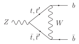
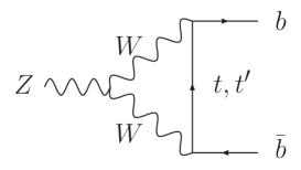
Figure 3: Modification of the $Z\to b\bar{b}$ rate from one-loop diagram including $t$ and $t^{\prime}$. In the case of a vector-like $t^{\prime}$, also the flavor changing neutral vertex $Ztt^{\prime}$ contributes.

2.2 The case for a fourth generation

Another possible extension of the CKM structure of SM is the addition of a fourth generation. In this case, the presence of $b^{\prime}$ implies a unitary $V_{4\times 4}$ mixing matrix such that tree-level FCNCs in hadronic $Z^{0}$ decays are now forbidden (see Eq. (14)). Next, we shall discuss the $(V_{td},V_{ts},V_{tb})$ bounds for this model.

Neglecting again the CP-violating phases beyond CKM, the $4\times 4$ unitary matrix contains three extra mixings which we parametrize, following Ref. [16], as

$${\bf V}_{4\times 4}=R_{34}(\theta_{u})R_{24}(\theta_{v})R_{14}(\theta_{w})\left(\begin{array}[]{cc}{\bf V_{3\times 3}^{(0)}}&{\bf 0}_{3\times 1}\\ {\bf 0}_{1\times 3}&1\\ \end{array}\right)\,,$$ (31)

where $R_{ij}(\theta)$ is the rotation in the $i-j$ flavour plane. It is important to notice that for the $3\times 3$ unitarity matrix part, ${\bf V_{3\times 3}^{(0)}}$, the usual Wolfenstein’s expansion is applicable irrespective to the size of $\theta_{u,v,w}$ in this particular parametrization. We then obtain (for $i=d,s,b$)

$$V_{ui} = \cos\theta_{w}V_{ui}^{(0)}$$ (32)

$$V_{ci} = \cos\theta_{v}V_{ci}^{(0)}-\sin\theta_{v}\sin\theta_{w}V_{ui}^{(0)}$$ (33)

$$V_{ti} = \cos\theta_{u}V_{ti}^{(0)}-\sin\theta_{u}\sin\theta_{v}V_{ci}^{(0)}-\sin\theta_{u}\cos\theta_{v}\sin\theta_{w}V_{ui}^{(0)}$$ (34)

$$V_{t^{\prime}i} = \sin\theta_{u}V_{ti}^{(0)}+\cos\theta_{u}\sin\theta_{v}V_{ci}^{(0)}+\cos\theta_{u}\cos\theta_{v}\sin\theta_{w}V_{ui}^{(0)}.$$ (35)

Using the fact that $(V_{ud}^{(0)},V_{us}^{(0)},V_{cd}^{(0)},V_{cs}^{(0)})$ are written in terms of the single parameter $\lambda$ up to ${\mathcal{O}}(\lambda^{3})$, the $4\times 4$ unitarity condition immediately constrains the two extra mixing angles appearing in Eqs. (32) and (33). The experimental values given in Ref. [1] indeed imply

$$|\theta_{w}|\leq{\mathcal{O}}(\lambda^{2}),\quad|\theta_{v}|\leq{\mathcal{O}}(\lambda)\,.$$ (36)

2.2.1 Current constraints on $V_{ti}$

Similarly to the vector-like model, the mixing angle $\theta_{u}$ is not constrained from the unitarity condition since the third row is not known. Given the hierarchy of Eq. (36), let us neglect $\theta_{w}$. However, even a small value of $\theta_{v}$ could entail a large deviation of $V_{ti}$ from its SM value. By choosing maximal $t-t^{\prime}$ mixing, i.e., $\theta_{u}=\pi/4$, Eq. (34) reduces to;

$$\begin{array}[]{lll}\sqrt{2}V_{td}=\underbrace{V_{td}^{(0)}}_{{\mathcal{O}}(\lambda^{3})}+\sin\theta_{v}\underbrace{V_{cd}^{(0)}}_{{\mathcal{O}}(\lambda)},&\sqrt{2}V_{ts}=\underbrace{V_{ts}^{(0)}}_{{\mathcal{O}}(\lambda^{2})}+\sin\theta_{v}\underbrace{V_{cs}^{(0)}}_{{\mathcal{O}}(1)},&\sqrt{2}V_{tb}=\underbrace{V_{tb}^{(0)}}_{{\mathcal{O}}(1)}+\sin\theta_{v}\underbrace{V_{cb}^{(0)}}_{{\mathcal{O}}(\lambda^{2})}\,.\end{array}$$ (37)

We notice that $(|V_{td}|,|V_{ts}|)$ can be enhanced as much as $({\mathcal{O}}(\lambda^{2}),{\mathcal{O}}(\lambda))$ for $|\theta_{v}|\simeq{\mathcal{O}}(\lambda)$. In such a case, $R$ value can be as low as:

$$R=\frac{1}{{\mathcal{O}} (\lambda^{2})+1}\simeq 0.95\,.$$ (38)

Combining Eq. (37) with the $4\times 4$ unitarity constraint in Eq. (36), we find that the largest possible deviation from the SM value of $V_{ti}$ is obtained for $|\theta_{v}|\simeq 0.2$ and $|\theta_{u}|\simeq 0.7$, i.e.,

$$|V_{td}|\raise 1.29167pt\hbox{$\;<$\kern-7.5pt\raise-4.73611pt\hbox{$\sim\;$}}0.03,\quad|V_{ts}|\raise 1.29167pt\hbox{$\;<$\kern-7.5pt\raise-4.73611pt\hbox{$\sim\;$}}0.2,\quad|V_{tb}|\raise 1.29167pt\hbox{$\;>$\kern-7.5pt\raise-4.73611pt\hbox{$\sim\;$}}0.8\,,$$ (39)

if we fix the other Wolfenstein parameters in ${\bf V_{3\times 3}^{(0)}}$ as $\lambda=0.22$ and $A=0.85$.

\psfrag{x}[c][c][0.9]{$\cos\theta_{u}$}\psfrag{y}[c][c][1]{\rotatebox{270.0}{$\frac{m_{t^{\prime}}}{m_{t}}$}}\psfrag{one}[c][c][0.8]{1\ $\sigma$}\psfrag{ninty}[c][c][0.8]{90\% C.L.}\psfrag{nintyfive}[c][c][0.8]{95\% C.L.}\psfrag{tpmass}[c][c][1]{\rotatebox{270.0}{$\leftarrow$} }\psfrag{1.2}[c][c][0.7]{1.2}\psfrag{1.4}[c][c][0.7]{1.4}\psfrag{1.6}[c][c][0.7]{1.6}\psfrag{1.8}[c][c][0.7]{1.8}\psfrag{2}[c][c][0.7]{2.0\ \ }\psfrag{-0.75}[c][c][0.7]{-0.75}\psfrag{-0.5}[c][c][0.7]{-0.50}\psfrag{-0.25}[c][c][0.7]{-0.25}\psfrag{0}[c][c][0.7]{0}\psfrag{1}[c][c][0.9]{\ }\psfrag{0.75}[c][c][0.7]{0.75}\psfrag{0.5}[c][c][0.7]{0.50}\psfrag{0.25}[c][c][0.7]{0.25}\psfrag{tv1}[c][c][0.8]{{$\theta_{v}=0.2$}}\psfrag{tv2}[c][c][0.8]{{$\theta_{v}=0.1$}}\includegraphics[width=227.62204pt]{4g1.eps}

(a)

\psfrag{x}[c][c][0.9]{$\cos\theta_{u}$}\psfrag{y}[c][c][1]{\rotatebox{270.0}{$\frac{m_{t^{\prime}}}{m_{t}}$}}\psfrag{one}[c][c][0.8]{1\ $\sigma$}\psfrag{ninty}[c][c][0.8]{90\% C.L.}\psfrag{nintyfive}[c][c][0.8]{95\% C.L.}\psfrag{tpmass}[c][c][1]{\rotatebox{270.0}{$\leftarrow$} }\psfrag{1.2}[c][c][0.7]{1.2}\psfrag{1.4}[c][c][0.7]{1.4}\psfrag{1.6}[c][c][0.7]{1.6}\psfrag{1.8}[c][c][0.7]{1.8}\psfrag{2}[c][c][0.7]{2.0\ \ }\psfrag{-0.75}[c][c][0.7]{-0.75}\psfrag{-0.5}[c][c][0.7]{-0.50}\psfrag{-0.25}[c][c][0.7]{-0.25}\psfrag{0}[c][c][0.7]{0}\psfrag{1}[c][c][0.9]{\ }\psfrag{0.75}[c][c][0.7]{0.75}\psfrag{0.5}[c][c][0.7]{0.50}\psfrag{0.25}[c][c][0.7]{0.25}\psfrag{tv1}[c][c][0.8]{{$\theta_{v}=0.2$}}\psfrag{tv2}[c][c][0.8]{{$\theta_{v}=0.1$}}\includegraphics[width=227.62204pt]{4g2.eps}

(b)

Figure 4: Excluded ranges for the mass and mixing of a fourth generation $t^{\prime}$ quark from the $B\to X_{s}\gamma$ branching ratio at 95%, 90% and 68.3% C.L. The dashed line indicates the experimental bound on $m_{t^{\prime}}$ (see Eq. (20)). We fix the mixing angles $\theta_{w}=0$ and $\theta_{v}\simeq 0.2,0.1$ for figure (a), (b). Constraints from $R_{b}$ are similar to those for a vector-like quarks, shown in Fig. 2b.

Next, we obtain constraints for $\theta_{v}$ and $\theta_{u}$ from a loop-level process, $B\to X_{s}\gamma$, by including the $t^{\prime}$ contribution. The result is shown in Fig. 4. In Fig. 4a, we fix $\theta_{v}=0.2$, the maximum allowed value from the unitarity condition, and find that the allowed range of $V_{tb}$ at $1\sigma$ (95% C.L.) is $0.07(-0.07)<V_{tb}<0.38(0.58)$. This interval does not overlap with the theoretically allowed region $|V_{tb}|\raise 1.29167pt\hbox{$\;>$\kern-7.5pt\raise-4.73611pt\hbox{$\sim\;$}}0.71$, Eq. (13), and therefore $|\theta_{v}|\simeq 0.2$ is excluded. In Fig. 4b, where $\theta_{v}=0.1$, we find that $V_{tb}$ above 0.11 is allowed.

Finally, we consider the constraints from the EW precision data. The large value of the $S$ parameter in the fourth generation model is often advocated to exclude this possibility. However, those analyses are usually performed assuming $T\simeq 0$. As was shown in the previous section, the $T$ parameter can be modified significantly in our case due to the mixing between the fourth generation fermions and the standard fermions (non-zero $\theta$). Assuming the new $b^{\prime}$ mass equal to the $t^{\prime}$ mass, which ensures a minimal $T$ value, we obtain

$$T>2.0\sin^{2}\theta,\quad U>0.17\sin^{2}\theta,\quad S>0.16,$$ (40)

to be compared with the results of the electroweak fit, $S=0.07\pm 0.10$, and $T=0.13\pm 0.10$ for $U=0$ [14]. In fact, a larger value of $S$ allows a larger value of $T$. Thus, this model is still viable for mixing angle and mass configurations similar to the previous model.

Once again, the ratio $R_{b}$ turns out to give the strongest constraints. Here, $t$ and $t^{\prime}$ loop corrections to $\Gamma(Z\to b\bar{b})$ imply

$$R_{b}\raise 1.29167pt\hbox{$\;<$\kern-7.5pt\raise-4.73611pt\hbox{$\sim\;$}}(1-0.019\sin^{2}\theta)R_{b}^{\rm SM}.$$ (41)

This bound, very similar to the one derived for the vector-like $t^{\prime}$ case, Eq.(27), requires (at 95% C.L.)

$$|\cos\theta_{u}|\raise 1.29167pt\hbox{$\;>$\kern-7.5pt\raise-4.73611pt\hbox{$\sim\;$}}0.93$$ (42)

and definitely closes the unnatural window $|\cos\theta_{u}|\raise 1.29167pt\hbox{$\;<$\kern-7.5pt\raise-4.73611pt\hbox{$\sim\;$}}1/\sqrt{2}$ left over by $B\to X_{s}\gamma$ (see Fig. 4).

We should also mention that gauge anomaly cancellation requires the same number of generations in the lepton and quark sectors. The fourth generation lepton contributions can also modify the above predictions quite significantly, depending on their masses (see the detailed discussion in Ref. [17]).

2.2.2 Impact on the single top production

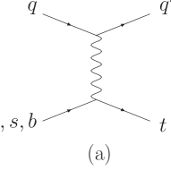
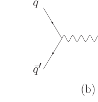
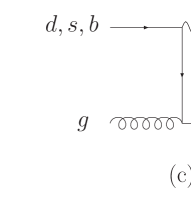
Figure 5: Representative diagrams for single top production: $t$-channel (a), $s$-channel (b), and $W$-associated production (c).

If $|V_{td}|$ and $|V_{ts}|$ are larger than their SM values, a possibility which could occur in the fourth generation model but not in the vector-like model, both the top branching ratios into $Wj$ and the single top production cross section for the $t$-channel and $W$-associated production ($Wt$) will be affected (see Fig. 5). It is interesting to check what kind of constraints the present limits on the single top production from the Tevatron give on the $V_{ti}$ matrix elements and what the prospects will be at the LHC. The cross sections for the $t$-channel production is proportional to the parton distribution functions for the incoming quark times the corresponding CKM element squared, i.e.,

$$\sigma(pp(p\overline{p})\to tj)=|V_{td}|^{2}\sigma_{d}^{\rm t-ch}+|V_{ts}|^{2}\sigma_{s}^{\rm t-ch}+|V_{tb}|^{2}\sigma_{b}^{\rm t-ch}\,,$$ (43)

similarly for the $W$-associated production, while the $s$-channel can be written as:

$$\sigma(pp(p\overline{p})\to tq;\ \ q=d,s,b)=(|V_{td}|^{2}+|V_{ts}|^{2}+|V_{tb}|^{2})\,\sigma^{\rm s-ch}\,.$$ (44)

In Table 1 the results for the cross sections calculated at LO with MadGraph/MadEvent [18] ($m_{t}=175$ GeV, $\mu_{R}=\mu_{F}=m_{t}$, PDF=CTEQ6L1 [19]) at the Tevatron and LHC are given as coefficients of the corresponding CKM matrix element. If the three-family unitarity holds, the contributions coming from the strange and down quarks are suppressed by the smallness of the corresponding CKM elements and give a negligible contribution to the total cross section.

Collider	Process	Cross section (pb)
		$|V_{tb}|^{2}$	$|V_{ts}|^{2}$	$|V_{td}|^{2}$
	$t$-channel	0.88	2.7	10.5
Tevatron	$s$-channel	0.30
	$Wt$	0.038	0.150	1.26
	$t$-channel	150(87)	277 (172)	766 (253)
LHC	$s$-channel	4.6 (3.4)
	$Wt$	30	67	294 (107)

Table 1: Contributions to the cross section for single top production proportional to the corresponding CKM element squared. Cross sections (in pb) are calculated at LO ($m_{t}=175$ GeV, $\mu_{R}=\mu_{F}=m_{t}$, PDF=CTEQ6L1 [19]) and refer to the production of a top. The anti-top cross sections are given in parenthesis when different from those of a top.

The above predictions can be compared to the most stringent limits from the CDF collaboration [20]:

$$\sigma^{\rm s-ch}_{\rm SM}+\sigma^{\rm t-ch}_{\rm SM} < 3.4\ {\rm pb\ at}\ 95\%\ {\rm C.L.}$$

$$\sigma^{\rm s-ch}_{\rm SM} < 3.1\ {\rm pb\ at}\ 95\%\ {\rm C.L.}$$ (45)

$$\sigma^{\rm t-ch}_{\rm SM} < 3.2\ {\rm pb\ at}\ 95\%\ {\rm C.L.}$$

These limits assume a SM scenario, with $V_{tb}=1$. In order to curb the large background coming mainly from $W+jets$ and $t\bar{t}$, the experimental analysis makes extensive use of the kinematical information of the signal, such as the presence of forward jet and/or of a charge asymmetry in the $t$-channel. However, the most important selection criterium is given by the requirement of two jets, of which one or two are $b$-tagged. If $V_{tb}=1$, the $t$-channel typically leads to one $b$-jet in the final state (from the top decay), while the $s$-channel to two $b$-jets. For sake of argument we restrict the following study to this distinctive feature, keeping in mind that the results obtained here are meant as illustration and could be easily improved by a more detailed analysis.

In this approximation, the limits on $\sigma^{\rm s-ch}_{\rm SM}$ and $\sigma^{\rm t-ch}_{\rm SM}$ can be translated into the cross section involving one $b$-jet, $\sigma_{1b}$, and two $b$-jets $\sigma_{2b}$ and their sum, $\sigma_{tot}=\sigma_{1b}+\sigma_{2b}$, where

$$\sigma_{1b} = R\left\{2(|V_{td}|^{2}+|V_{ts}|^{2})\sigma^{\rm s-ch}+[|V_{td}|^{2}\sigma_{d}^{\rm t-ch}+|V_{ts}|^{2}\sigma_{s}^{\rm t-ch}+|V_{tb}|^{2}\sigma_{b}^{\rm t-ch}]\right\}\,,$$ (46)

$$\sigma_{2b} = R\,|V_{tb}|^{2}\,\sigma^{\rm s-ch}.$$ (47)

$R$ is defined in Eq. (4). Using the constraints in Eq. (45) and the result $R>0.61$ at 95% C.L., we obtain the excluded regions for $|V_{ti}|$ as shown in Fig. 6. The resulting allowed values, $|V_{td}|\raise 1.29167pt\hbox{$\;<$\kern-7.5pt\raise-4.73611pt\hbox{$\sim\;$}}0.46$ and $|V_{ts}|\raise 1.29167pt\hbox{$\;<$\kern-7.5pt\raise-4.73611pt\hbox{$\sim\;$}}0.62$, are much less constrained than those obtained from the $4\times 4$ unitarity and $B\to X_{s}\gamma$.

\psfrag{Vtd}[c][c][0.8]{$|V_{td}|$}\psfrag{Vts}[c][c][0.8]{$|V_{ts}|$}\psfrag{Vtb}[c][c][0.8]{$|V_{tb}|$}\psfrag{0.8}[c][c][0.7]{0.8}\psfrag{0.6}[c][c][0.7]{0.6}\psfrag{0.4}[c][c][0.7]{0.4}\psfrag{0.2}[c][c][0.7]{0.2}\psfrag{1}[r][c][0.7]{1.0}\psfrag{R}[c][c][.9]{$R$}\psfrag{ST}[c][c][.9]{\small single top}\psfrag{physical}[c][c][.9]{\small physical $\longrightarrow$}\psfrag{all}[c][c][.9]{\small combined $\to$}\epsfbox{fig1.eps}\psfrag{Vtd}[c][c][0.8]{$|V_{td}|$}\psfrag{Vts}[c][c][0.8]{$|V_{ts}|$}\psfrag{Vtb}[c][c][0.8]{$|V_{tb}|$}\psfrag{0.8}[c][c][0.7]{0.8}\psfrag{0.6}[c][c][0.7]{0.6}\psfrag{0.4}[c][c][0.7]{0.4}\psfrag{0.2}[c][c][0.7]{0.2}\psfrag{1}[r][c][0.7]{1.0}\psfrag{R}[c][c][.9]{$R$}\psfrag{ST}[c][c][.9]{\small single top}\psfrag{physical}[c][c][.9]{\small physical $\longrightarrow$}\psfrag{all}[c][c][.9]{\small combined $\to$}\epsfbox{fig2.eps}\psfrag{Vtd}[c][c][0.8]{$|V_{td}|$}\psfrag{Vts}[c][c][0.8]{$|V_{ts}|$}\psfrag{Vtb}[c][c][0.8]{$|V_{tb}|$}\psfrag{0.8}[c][c][0.7]{0.8}\psfrag{0.6}[c][c][0.7]{0.6}\psfrag{0.4}[c][c][0.7]{0.4}\psfrag{0.2}[c][c][0.7]{0.2}\psfrag{1}[r][c][0.7]{1.0}\psfrag{R}[c][c][.9]{$R$}\psfrag{ST}[c][c][.9]{\small single top}\psfrag{physical}[c][c][.9]{\small physical $\longrightarrow$}\psfrag{all}[c][c][.9]{\small combined $\to$}\epsfbox{fig3.eps}

Figure 6: Excluded regions for $|V_{td}|$, $|V_{ts}|$, and $|V_{tb}|$ as obtained from the CDF limits on the single top production, $\sigma_{1b}$ (orange) and $\sigma_{1b}+\sigma_{2b}$(dark-blue), the measurements of $R$ (pink) and the physical bound $|V_{td}|^{2}+|V_{ts}|^{2}+|V_{tb}|^{2}<1$ (yellow). The combination of these four bounds provides an additional excluded region (light-blue).

3 Future prospects at the LHC

In this section we discuss the perspectives for the determination of $V_{tb}$ at the LHC. The primary method to extract information on $V_{tb}$ will be through the measurement of the single top cross sections, which are directly proportional to $|V_{tb}|^{2}$. The best determination will come from $t$-channel production, but it will still be crucial to have measurements from all the three channels to identify possible sources of new physics, since in general new models may have effects in one channel and not in the others [21]. For the models introduced in the previous section, it will also be possible to study the production of extra heavy quarks and from that to discriminate, for instance, the case of just one vector-like top from that of a full $SU(2)_{L}$ doublet. We briefly illustrate this possibility and outline possible strategies in Section 3.2. We mention in passing that another handle to $V_{tb}$ might be offered by the direct measurement of the top width. There have been suggestions on how to perform such a measurement in $e^{+}e^{-}$ experiments [22, 23]. We do not discuss this possibility here, even though such studies at the hadron colliders would be certainly welcome.

3.1 $V_{tb}$ measurement at the LHC

Going from Tevatron to LHC, the higher energy and luminosity provide better possibilities for a precise determination of the CKM matrix element $V_{tb}$, in all the three production modes: $t$-channel ($q^{2}_{\mathrm{W}}<0$), $s$-channel ($q^{2}_{\mathrm{W}}>0$), and $W$-associated production ($q^{2}_{\mathrm{W}}$=$M^{2}_{\mathrm{W}}$). The corresponding cross sections are shown in Table 2 [24, 25, 26].

Process	$\sigma$ (pb)
$t$-channel	245
$Wt$	60
$s$-channel	10

Table 2: The single top production cross section values at the LHC at the NLO level (top and anti-top contributions are summed).

The three production processes occupy different phase space regions and have large differences in signal-to-background ratios.

3.1.1 Determination of $V_{tb}$ from the $t$-channel production

For the $t$-channel, the signature is one lepton, missing energy, one $b$-jet and one recoil jet (un-tagged and at high rapidity). In the CMS study of Ref. [27] it is shown that a signal-to-background ratio higher than unity is achievable and the main background after selection is $t\bar{t}$.

The total relative uncertainty on the cross section can be estimated by:

$$\frac{\Delta\sigma}{\sigma}=\frac{\sqrt{N_{S}+N_{B}}}{N_{S}}\oplus\frac{\Delta N_{S}\oplus\Delta N_{B}}{N_{S}}\oplus\frac{\Delta L}{L},$$ (48)

where $N_{S}$ and $N_{B}$ are the number of selected signal and background events respectively, and $L$ and $\Delta L$ are the LHC luminosity and its uncertainty. $\Delta N_{S}$ and $\Delta N_{B}$ are the experimental systematics (such as uncertainties on jet energy scale and $b$-tagging efficiency) for the signal and the background, respectively. In the latter the uncertainty on the background sample normalization is also included. Fig. 7 shows its dependence on the signal cross section. For 10 fb^-1 of integrated luminosity and under the assumption that the signal cross section is as expected in SM, this results in

$$\frac{\Delta\sigma}{\sigma} = \pm 3\%{\rm(stat.)}\pm 7\%{\rm(syst.)}\pm 5\%{\rm(lum.)}.$$ (49)

The measurement is systematics dominated, mostly due to the imperfect knowledge of jet energy scale, $b$-tagging efficiency and mistag probability.

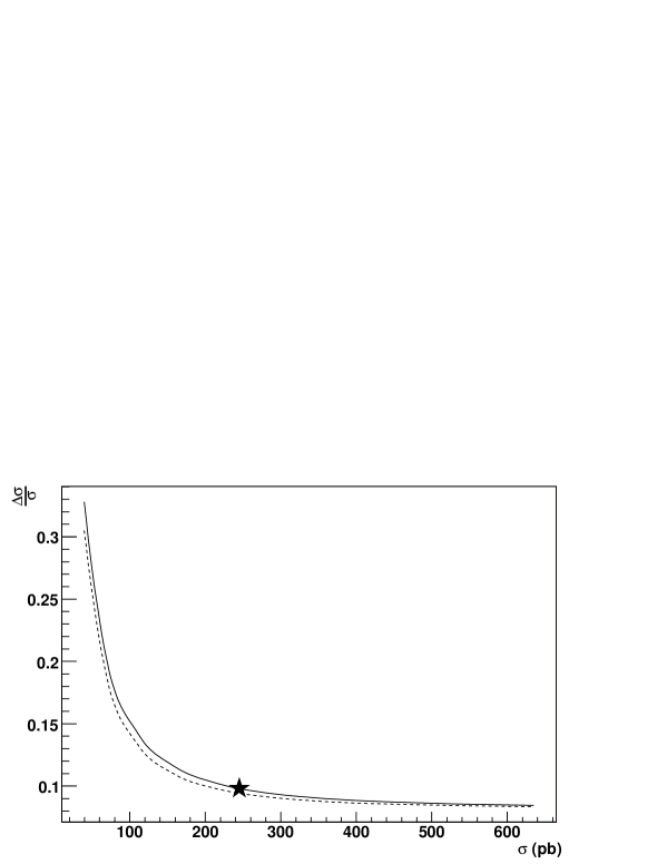
Figure 7: The relative uncertainty on the cross section as a function of the cross section for the $t$-channel, corresponding to 10 fb^-1 integrated luminosity (solid line). The star indicates the SM expectation. The dashed line represents the systematic uncertainty.

The expected uncertainty on $V_{tb}$ may be computed as

$$\frac{\Delta V_{tb}}{V_{tb}} = \frac{1}{2}\left(\frac{\Delta\sigma^{\rm meas}}{\sigma^{\rm meas}}\oplus\frac{\Delta\sigma^{\rm th}}{\sigma^{\rm th}}\right).$$ (50)

For the $t$-channel, the uncertainty on $\sigma^{\rm th}$ has been calculated in detail in Ref. [28] and has the following contributions:

• PDF uncertainties: $+1.3\%,-2.2\%$,

• higher orders (QCD scale): $3\%$,

• variation of the top mass within 2 GeV: $+1.56\%,-1.46\%$,

• uncertainty on the b-quark mass: $<1\%$.

The above uncertainties are associated to the fully inclusive cross section. Therefore, the overall uncertainty on $V_{tb}$ is estimated to be 5%. A more accurate determination would take into account the specific phase space region selected by the analyses. In particular, we point out that the request of exactly two jets (vetoing any other jet above a certain threshold), needed to reduce the $t\bar{t}$ background to a reasonable level, may give a larger scale dependence than quoted above.

Moreover, more studies are needed on the electroweak corrections. Due to the presence of the $W$ in the intermediate state, real and virtual photon emissions are expected to give sizable amplitudes, and the correction to $\sigma^{\rm th}$ might be as large as several percents [29].

3.1.2 Other single top processes

For the $W$-associated production, one can follow two complementary search strategies: one based on the selection of two isolated leptons, the other with one isolated lepton and two light jets compatible with the $W$ mass. In both cases missing energy and one $b$-jet are also required in the final state, and no other jet is allowed. The main limitation of this analysis is the similarity of the signal with the $t\bar{t}$ background, where the jet counting is the only handle to reduce it. It is worth mentioning that such a similarity with the $t\bar{t}$ is also a problem at the theoretical level: $Wt$ is consistently defined and insensitive to the quantum interference with $t\bar{t}$ only when extra $b$-jets in the final state are vetoed [26].

After the selection, a signal-to-background ratio of 0.37 is expected for the di-leptonic channel and 0.18 for the single-leptonic, the background being almost completely constituted by $t\bar{t}$ events. In order to constrain this background, and to cancel out a large part of the main systematics, one can make use of a control sample and employ the so-called “ratio method” [30]. Then, the cross section can be rewritten as

$$\sigma^{Wt}=\frac{R_{tt}(N-B_{0})-(N_{c}-B_{c})}{\epsilon^{Wt}(R_{tt}-R_{Wt})}$$ (51)

where $N(B_{0})$ and $N_{c}(B_{c})$ are the total number of selected events (the non-$t\bar{t}$ background) in the main and in the control samples, respectively. $\epsilon^{Wt}$ is the signal selection efficiency. $R_{Wt}(R_{tt})$ is the ratio of the efficiency in the control sample to the efficiency in the main sample for the signal (and $t\bar{t}$). The uncertainty in the background sample normalization, which dominates $\Delta N_{B}$ in Eq. (48), is now associated to the statistical uncertainty in the large control sample of $N_{c}$ and the systematic uncertainty due to the background rejection is highly reduced since it only enters in the ratio.

The expected precision on the cross section with 10 fb^-1 of integrated luminosity is:

$$\frac{\Delta\sigma}{\sigma}=\pm 6\%{\rm(stat.)}\pm 16\%{\rm(syst.)}\pm 5\%{\rm(lum.)}.$$ (52)

This result is obtained by averaging di-leptonic and single-leptonic analyses from Ref. [30] assuming fully correlated systematic uncertainty. The statistical significance for 10 fb^-1 is higher than six standard deviations.

Although not competitive with the $t$-channel production in terms of the achievable precision in the extraction of $V_{tb}$, the $W$-associated process is still attractive since the observation of the $W$ in the final state would prove that the top is produced through a charged current interaction. As we mentioned above, the definition and the measurement of this channel is difficult due to the large overlap in phase space with $t\bar{t}$, whose cross section is more than ten times larger. In this respect it is interesting to note that in $\gamma p$ collisions at the LHC, where protons emit almost real photons colliding with protons of the opposite beam, the $Wt$ and $t\bar{t}$ cross sections are of a similar size, leading to a much better signal over background ratio. Work to explore this alternative is on-going [31].

For the $s$-channel process $q\bar{q}^{\prime}\to W^{*}\to t\bar{b}/\bar{t}b$, whose signature is one lepton, missing energy and two $b$-jets, the $t\bar{t}$ background is again difficult to curb and a ratio method has to be applied as in the $Wt$ case. The final result of the analysis [27], for 10 fb^-1, is:

$$\frac{\Delta\sigma}{\sigma} = \pm 18\%{\rm(stat.)}\pm 31\%{\rm(syst.)}\pm 5\%{\rm(lum.)},$$ (53)

where most of the contribution to the systematics comes from the jet energy scale uncertainty.

3.2 $t^{\prime}$ production cross sections at the LHC

If extra quarks exist, either as a $SU(2)$ gauge singlet or in a doublet, and they are light enough, they could be also discovered at LHC. The phenomenology of such states has been studied in the literature (see, e.g., Refs. [9, 32]) and here we limit ourselves to a brief discussion, highlighting how the $SU(2)$ nature of the extra quark(s) could be determined.

In Figs. 9 and 9 the $t^{\prime}$ production cross sections are shown for various production modes as a function of the $t^{\prime}$ mass. For simplicity, we have set $|V_{t^{\prime}b}|=|({\bf VV^{\dagger}})_{tt^{\prime}}|=1$, so that if the mass of the $t^{\prime}$ is equal to the top mass ($\sim 175$ GeV) the cross sections are equal to the SM cross sections for top production. Results at LO have been obtained with MadGraph/MadEvent [18], while MCFM [33] has been used when calculations at next-to-leading order in QCD were available.

In Fig. 9 the double $t^{\prime}$ production cross section is given by the solid line and the single $t^{\prime}$ production channels are given by the dashed ($s$-channel), dash-dotted ($t$-channel) and dotted ($Wt^{\prime}$) lines. For $t^{\prime}$ masses below $\sim 250$ GeV double $t^{\prime}$ production dominates the single $t^{\prime}$ production, just as the double top cross section is larger than the single top in SM. Above $\sim 250$ GeV the $t$-channel becomes the dominant production mechanism, as it is the least dependent on the $t^{\prime}$ mass. Note, however, that the single $t^{\prime}$ production scales as $|V_{t^{\prime}b}|^{2}$, while the pair production cross section is independent of it and might still be the dominant production mechanism. For example, for $\cos\theta=0.71$ the single $t^{\prime}$ production cross sections decrease by an overall factor of four.

One way to distinguish between a new extra doublet and a vector-like quark is to look for FCNCs, which are only present for the vector-like case. At leading order there are two mechanisms for the production of a $t\bar{t}^{\prime}/t^{\prime}\bar{t}$ pair, viz., through an $s$-channel $Z$ or Higgs boson. The total cross section for the processes $pp\rightarrow Z\rightarrow t\bar{t}^{\prime}/\bar{t}t^{\prime}$ and $gg\rightarrow H\rightarrow\bar{t}t^{\prime}/t\bar{t}^{\prime}$ are given by the solid and the dotted lines in Fig. 9, respectively. Note that the $gg\rightarrow H\rightarrow\bar{t}t^{\prime}/t\bar{t}^{\prime}$ cross section is almost independent of the $t^{\prime}$ mass because of the cancellation of two competing effects, i.e., the increase of the $tt^{\prime}H$ coupling and the gluon luminosity suppression for larger $x$.

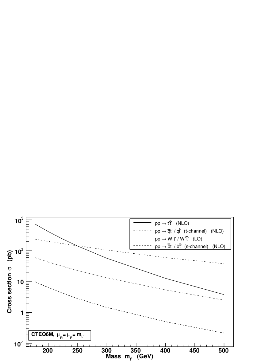
Figure 8: $t^{\prime}$ production as a function of its mass, with $|V_{bt^{\prime}}|$ and $|({\bf VV^{\dagger}})_{tt^{\prime}}|$ set to one. Results are shown for $t^{\prime}\bar{t}^{\prime}$ pair production and the three single $t^{\prime}$ channels.

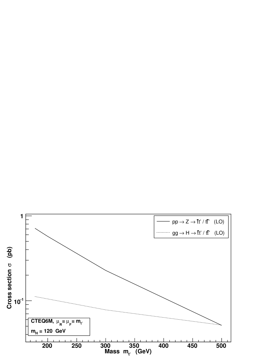
Figure 9: FCNC $\bar{t}t^{\prime}/t\bar{t}^{\prime}$ production through an $s$-channel $Z$ or Higgs boson (solid and dotted lines) as a function of the mass of the $t^{\prime}$, with $|({\bf VV^{\dagger}})_{tt^{\prime}}|$ set to one.

4 Conclusions

In this paper we have elaborated on the phenomenology concerning the CKM matrix element $V_{tb}$ in models that relax the strong constraints coming from the unitarity. We have first emphasized that $V_{tb}\simeq 1$ is required neither from $B$ physics nor from the top quark decay rate measurements. Only the direct extraction of $V_{tb}$ from the single top production cross section at the Tevatron and at the LHC will allow to complete our knowledge of the CKM matrix and hopefully shed new light on the nature of the top quark.

As a simple extension of the SM that breaks the $3\times 3$ unitarity condition of the CKM matrix and leads to a deviation from $V_{tb}\simeq 1$, we have considered the addition of extra fermions: either a vector-like up-type quark ($t^{\prime}$) or fourth generation quarks ($t^{\prime}$ and $b^{\prime}$). The main motivation for selecting these models is that they serve well the illustrative purpose of our study. They are simple, self-consistent and allow to easily find the constraints on $V_{tb}$ coming both from precision physics and direct observation. In this respect, they should be regarded as useful templates for further experimental scrutiny on $V_{tb}$.

We find that the strongest constraint on these models comes from $R_{b}$, which severely restricts the allowed amount of $t-t^{\prime}$ mixing. When this result is combined with the very recent direct bound on the $t^{\prime}$ mass by the CDF collaboration, $m_{t^{\prime}}\raise 1.29167pt\hbox{$\;>$\kern-7.5pt\raise-4.73611pt\hbox{$\sim\;$}}258$ GeV, one finds $|V_{tb}|>0.9$. This very strong bound relies, however, on two assumptions which might not hold in more sophisticated models. The first one is that the corrections to $R_{b}$ induced by loop effects are only coming from the $t^{\prime}$ contribution, and therefore models with an extended particle content may be less constrained. The second assumption, which is at the basis of the lower bound on the $t^{\prime}$ mass by CDF, is that the branching ratio of $t^{\prime}\to Wq$ is one. For instance, this condition is satisfied in our vector-like $t^{\prime}$ model only for $m_{t^{\prime}}\raise 1.29167pt\hbox{$\;<$\kern-7.5pt\raise-4.73611pt\hbox{$\sim\;$}}300$ GeV. If at least one of the above conditions is not fulfilled, we have shown that other indirect measurements, such as those coming from $B\to X_{s}\gamma$ or the $S,T,U$ oblique parameters should also be considered.

In the near future the observation of the single top process, which is challenging both at the Tevatron and the LHC, will for the first time provide a direct measurement of $V_{tb}$. We showed that the current lower bound from Tevatron data has started giving direct information on the magnitudes of $V_{td}$ and $V_{ts}$, and that they will be further constrained as soon as the LHC data will be available. Among all three possible production mechanisms, the $t$-channel is the most promising process where $V_{tb}$ could be determined at the 5% precision level already with 10 fb^-1 of integrated luminosity. The precision of this result is limited by the systematic uncertainty and might be well improved with better understanding of the detector and background. The other channels, $W-$associated and $s$-channel, are more challenging due to a much larger systematic uncertainty. However, a measurement of these production mechanisms will be important to complete our knowledge of the top quark coupling to the weak current and possibly reveal new physics.

References

• [1] S. Eidelman et al. [Particle Data Group], Phys. Lett. B 592 (2004) 1.
• [2] V. M. Abazov et al. [D0 Collaboration], arXiv:hep-ex/0603029.
• [3] CDF Collaboration, http://www-cdf.fnal.gov/physics/new/bottom/060406.blessed-Bsmix/
• [4] M. Okamoto, PoS LAT2005 (2006) 013 [arXiv:hep-lat/0510113].
• [5] D. Acosta et al. [CDF Collaboration], Phys. Rev. Lett.  95 (2005) 102002 [arXiv:hep-ex/0505091].
• [6] V. M. Abazov et al. [D0 Collaboration], arXiv:hep-ex/0603002.
• [7] P. Candelas, G. T. Horowitz, A. Strominger and E. Witten, Nucl. Phys. B 258 (1985) 46.
J. L. Hewett and T. G. Rizzo, Phys. Rept.  183 (1989) 193.
F. Del Aguila and J. Santiago, JHEP 0203 (2002) 010 [arXiv:hep-ph/0111047].
N. Arkani-Hamed, A. G. Cohen, E. Katz, A. E. Nelson, T. Gregoire and J. G. Wacker, JHEP 0208 (2002) 021 [arXiv:hep-ph/0206020].
• [8] CDF Collaboration,
http://www-cdf.fnal.gov/physics/new/top/2005/ljets/tprime/gen6/public.html
• [9] J. A. Aguilar-Saavedra, Phys. Lett. B 625 (2005) 234 [Erratum-ibid. B 633 (2006) 792] [arXiv:hep-ph/0506187].
• [10] A. J. Buras and M. K. Harlander, Adv. Ser. Direct. High Energy Phys.  10 (1992) 58.
• [11] A. L. Kagan and M. Neubert, Eur. Phys. J. C 7 (1999) 5 [arXiv:hep-ph/9805303].
• [12] K. G. Chetyrkin, M. Misiak and M. Munz, Phys. Lett. B 400 (1997) 206 [Erratum-ibid. B 425 (1998) 414] [arXiv:hep-ph/9612313].
• [13] L. Lavoura and J. P. Silva, Phys. Rev. D 47 (1993) 2046.
• [14] [ALEPH Collaboration, DELPHI Collaboration, L3 Collaboration, OPAL Collaboration, SLD Collaboration, LEP Electroweak Working Group, SLD Electroweak Group and SLD Heavy Flavour Group], arXiv:hep-ex/0509008.
• [15] P. Bamert, C. P. Burgess, J. M. Cline, D. London and E. Nardi, Phys. Rev. D 54 (1996) 4275 [arXiv:hep-ph/9602438].
• [16] F. J. Botella and L. L. Chau, Phys. Lett. B 168 (1986) 97.
• [17] V. A. Novikov, L. B. Okun, A. N. Rozanov and M. I. Vysotsky, JETP Lett.  76 (2002) 127 [Pisma Zh. Eksp. Teor. Fiz.  76 (2002) 158] [arXiv:hep-ph/0203132].
H. J. He, N. Polonsky and S. f. Su, Phys. Rev. D 64 (2001) 053004 [arXiv:hep-ph/0102144].
B. Holdom, arXiv:hep-ph/0606146.
• [18] F. Maltoni and T. Stelzer, JHEP 0302 (2003) 027 [arXiv:hep-ph/0208156].
• [19] J. Pumplin, D. R. Stump, J. Huston, H. L. Lai, P. Nadolsky and W. K. Tung, JHEP 0207 (2002) 012 [arXiv:hep-ph/0201195].
• [20] CDF Coll. Note 8185, April, 2006.
• [21] T. Tait and C. P. Yuan, Phys. Rev. D 63 (2001) 014018 [arXiv:hep-ph/0007298].
• [22] L. H. Orr, Y. L. Dokshitzer, V. A. Khoze and W. J. Stirling, arXiv:hep-ph/9307338.
• [23] P. Batra and T. M. P. Tait, arXiv:hep-ph/0606068.
• [24] M. C. Smith and S. Willenbrock, Phys. Rev. D 54 (1996) 6696 [arXiv:hep-ph/9604223].
• [25] T. Stelzer, Z. Sullivan and S. Willenbrock, Phys. Rev. D 56 (1997) 5919 [arXiv:hep-ph/9705398].
• [26] J. Campbell and F. Tramontano, Nucl. Phys. B 726 (2005) 109 [arXiv:hep-ph/0506289].
• [27] V. Abramov et al., CMS note 2006/084.
• [28] Z. Sullivan, Phys. Rev. D 70 (2004) 114012 [arXiv:hep-ph/0408049].
• [29] M. Beccaria, G. Macorini, F. M. Renard and C. Verzegnassi, arXiv:hep-ph/0605108.
• [30] K. F. Chen et al., CMS note 2006/086
• [31] K. Piotrzkowski et al., in preparation.
• [32] T. Han, H. E. Logan, B. McElrath and L. T. Wang, Phys. Rev. D 67 (2003) 095004 [arXiv:hep-ph/0301040].
• [33] J. M. Campbell and R. K. Ellis, Phys. Rev. D 60 (1999) 113006 [arXiv:hep-ph/9905386].